Distribution-Free Bayesian multivariate predictive inference
Abstract
We introduce a comprehensive Bayesian multivariate predictive inference framework. The basis for our framework is a hierarchical Bayesian model, that is a mixture of finite Polya trees corresponding to multiple dyadic partitions of the unit cube. Given a sample of observations from an unknown multivariate distribution, the posterior predictive distribution is used to model and generate future observations from the unknown distribution. We illustrate the implementation of our methodology and study its performance on simulated examples. We introduce an algorithm for constructing conformal prediction sets, that provide finite sample probability assurances for future observations, with our Bayesian model.
1 Introduction
The predictive distribution is an important feature of Bayesian analyses that is typically used as a diagnostic tool for assessing model fit. In this work we apply a hierarchical Bayesian model, that is a mixture of finite Polya trees corresponding to multiple dyadic partitions of , to a sample of iid observations from an unknown distribution . The resulting posterior predictive distribution is used to approximate the distribution of future observations from .
The use of finite Polya trees to define random distributions on dyadic partitions of the unit interval was introduced in Ferguson (1974). The theoretical properties of Polya tree models for density estimation has been widely studied. Use of Polya trees, corresponding to multiple dyadic partitions, for distribution-free estimation of multivariate densities was suggested in Wong and Ma (2010) and Ma (2017). The novel features of this work is the introduction of a hierarchical Bayesian model that assigns distributions to sets of dyadic partitions of ; the introduction and implementation of a comprehensive Bayesian predictive inference framework; the adaptation of the Vovk (2005) method for constructing Conformal prediction sets to Bayesian analyses.
In Section 2 we present our inferential framework. In Sections 3, 4, 5, we illustrate the use of our methodology and study its performance on simulated examples. In Section 3 we study how well our model approximates and estimates one-dimensional and two-dimensional densities. In Section 4 we apply our method for quantile regression for a two-dimensional density, and introduce and implement an algorithm for constructing Conformal prediction sets with our Bayesian model. In Section 5 we attempt to scale up our methodology to provide predictive inference for a sample of continuous variables and one categorical variable. In Section 6 we discuss our work and outline changes needed to make it applicable in high dimensional problems.
2 Hierarchical Bayesian modelling for predictive inference
2.1 Dyadic segmentations of the -dimensional unit cube
level dyadic segmentations are constructed by partitioning the unit cube, , times in half according to its dimensions. Each segmentation, , consists of subintervals specified by a segmentation ordering vector, with . The segmentation begins by partitioning according to Dimension into two halves, that consists of the small values of coordinate and that consists of the large values of coordinate . And then, for and , is partitioned in halve according to coordinate into consisting of small values of coordinate and into consisting of large values of coordinate .
In the segmentations we consider in the examples in this report, all the subintervals at the same level are partitioned according to the same dimension (i.e. is the same ). In which case, is given by .
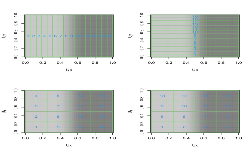
In Figure 1 we display four level dyadic segmentations of into subintervals. Setting the X axis to be Dimension 1 and the Y axis to be Dimension 2, the segmentation with all is denoted by ; the segmentation with all is denoted by ; while the segmentation with , , and is denoted . The numbers in each subinterval mark the positions of the level subintervals, , for each segmentation.

2.2 The hierarchical Beta model
The level hierarchical Beta (hBeta) model is a finite Polya tree model that generates random densities that are step functions on for a given level segmentation . The parameters of the hBeta model are Beta distribution hyper-parameters, and for and . The hBeta model generates the following components.
a. Independent Beta random variables. , for and . The Beta random variables specify the conditional subinterval probabilities. and . For and , and .
b. Subinterval probabilities. The subinterval probabilities, , are products of the conditional subinterval probabilities. and . For and , and .
c. Step function PDF. The components of specify the step function PDF,
| (1) |
for and with denoting the indicator function corresponding to subinterval .
In Figure 2 we provide a schematic for the hierarchical Beta model with levels.
2.3 The hierarchical Bayesian framework
Let denote the sample of iid observations from . On observing data points , our goal is to provide inference regarding an unobserved data point , that is assumed to be also independently sampled from . To drive our inferential framework, we elicit the following generative model for .
Definition 2.1 Generative model for data
-
1.
Sample with probability from a given set of level segmentations .
-
2.
Generate from the hBeta model with , for and .
-
3.
For , generate .
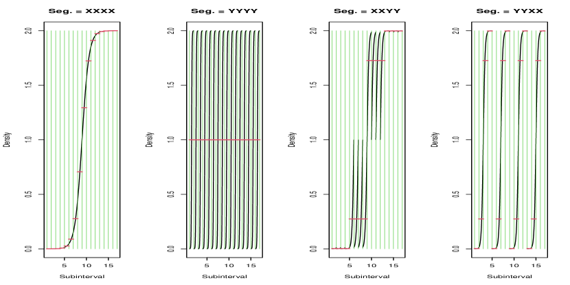
Example 2.2 In Figure 3 we display the distribution of the CDF of in Model 2.3, for the level segmentation of , with subintervals for , for . In Model 2.3, are iid with , therefore , and thus the expectation of is the density.
The plots reveal that increasing decreases the dispersion of . For , the probabilities in are concentrated – very unevenly – in a few very small clusters of contiguous subintervals. For , the distribution of is spread out in large clusters of similarly probable contiguous subintervals. While for , the distribution of consists of large clusters of low probability contiguous subintervals and a few small clusters of contiguous high probability subintervals.

2.3.1 The posterior data model
In this subsection we derive the conditional distribution given , of and the vector of Beta parameters, , for Model 2.3.
For , , , , let denote the indicator variable for the event . The number of observations in subinterval is . Conditional on , and . For and , conditioning on and on , and . Recalling that and denoting , this implies that .
Ferguson (1974) has already noted the conjugacy of the conditional distribution of given and for the hBeta model. In our inferential framework, the segmentation is random and we consider the conditional distribution of and given . Denoting and , we begin by deriving the conditional distribution of .
| (2) | |||||
where the equality in (2) is because and . The latter holds because given and , the components of are independently and Uniformly distributed within their respective level subintervals, and each level subintervals for each has volume . There are different indicator vector instances that yield the same counts vector . As the components of are exchangeable in Model 2.3 then each instance of is equally probable, threfore
| (3) |
Note that for each segmentation , , , and for and , and . Denoting , recursively invoking these relations we may express,
| (4) | |||||
Now that we have derived , we express the conditional distribution of ,
| (5) |
where is the conjugate posterior density of given and for the hBeta model.
Example 2.3 According to Expression (2), the conditional segmentation probability, , is proportional to the product of the reciprocal of the multinomial coefficient for the counts vector in (3) and the conditional probability of the counts vector, , which is determined by .
Recall that in Model 2.3 given and , is multinomial with sample size and probabilities vector . Thus the results of Example 2.3 suggest that for small values of large probabilities will be given to unevenly distributed counts vectors and that increasing will favour more evenly distributed counts vectors.
To illustrate the effect of on , in Table 1 we list conditional segmentation probabilities for a set of level segmentations, , and a sample of observations, , in the unit cube . The rows of Table 1 correspond to the segmentations, . The counts vector, , for is listed in Column 1. In columns 2-4, we list for .
Indeed, we see that increasing provides larger probabilities to the segmentations that yield more evenly distributed count vectors at the first rows of Table 1. Furthermore, comparing the second and third rows reveals that the segmentation probabilities is not exchangeable in , where for each value of , segmentations that yield contiguous non-zero counts are more probable. Yet, the two segmentations yielding counts vector with a single non-zero entry are equally probable.
| 0.00 | 0.01 | 0.13 | |
| 0.00 | 0.04 | 0.16 | |
| 0.01 | 0.07 | 0.19 | |
| 0.49 | 0.44 | 0.26 | |
| 0.49 | 0.44 | 0.26 |
2.4 Predictive inference
The predictive distribution is the distribution of for generative model 2.3. Let denote the density function for the predictive distribution, which is a mixture of for random and . The predictive probability of is given by
| (6) |
Let be a sufficiently small subset, so that it is a subset of a single level subinterval. As is constant on for all , then is constant on and therefore
And in general, is piecewise constant.
For , let denote the index of the level subinterval for segmentation that covers . Per construction and ,
for that is a product of . Therefore given and , we may express the conditional predictive probability of ,
| (7) |
As any Bayesian model, our inferential framework provides Bayesian estimates and credible regions for the model parameters. For predictive inference we further consider three types of outcomes:
a. Predictive samples. Predictive samples, , are iid samples from the predictive distribution. Predictive samples may be generated by repeating the following steps for : Sample , compute , sample .
b. Predictive probabilities. The predictive probability of is for generative model 2.3. This outcome may be numerically evaluated by computing the proportion of predictive samples in ,
In the next two subsections we analytically derive the predictive probability of .
c. Credible prediction sets. A level credible prediction set is with predictive probability . Thus the number predictive samples in is a random variable.
2.4.1 The prior predictive distribution
2.4.2 The posterior predictive distribution
The posterior predictive distribution of is the conditional distribution of given in generative model 2.3.
Conditional on and on , , with independent and for . Thus using (7) we may express
| (9) | |||||
with . Recalling that the sequence subinterval counts is decreasing, , let denote the largest with a nonzero count, i.e. . Therefore we may rewrite Expression (9),
| (10) | |||||
and thus for the conditional posterior predictive density is
| (11) |
2.5 Frequentist properties of our inferential framework
Recall, the underlying assumption in this report is that the real data generative model is that are iid . We will use subscript to denote real probabilities, all other probability statements are with respect to model 2.3.
We begin by considering a single segmentation . Let denote the vector of probabilities that assigns to subintervals . Thus the real sampling distribution of is Multinomial with number of trials and event probabilities vector . In our inferential framework, the real probability that is estimated by the conditional posterior predictive probability
To assess how well we evaluate with a given segmentation , we consider two types of errors: (a) approximation error, defined as the distance between and step-function density
| (15) |
which is an irreducible term that depends on the smoothness of with respect to ; (b) estimation error of by , which is reduced by increasing . The estimation error may be further divided into bias and variance terms.
In general, coarse segmentations have large approximation error and small estimation error. Refining the segmentation by increasing , decreases the approximation error and increases the estimation error. For coarse segmentation and sufficiently large that ensures that and thus , Expression (12) implies that for ,
Therefore for small and coarse segmentations has small bias.
On the other hand, if then according to Expression (11), for any segmentation that is a refinement of . As a result, our density estimators maintain small estimation error for fine segmentations. This is especially useful for larger values of that yield biased density estimation with small estimation variance. According to the simulations in Subsection 3.1, setting provide small estimation error even for fine segmentations and small .
Our inferential framework considers multiple segmentations , with different approximation and estimation errors, that are weighted according to the posterior segmentation probability . The most interesting and surprising feature of our framework is that for segmentations with large posterior probabilities tend to have small approximation and estimation errors. We will demonstrate this in simulations in Subsection 3.2.
Our inferential framework also produces level credible prediction sets, . Per construction, credible prediction sets have posterior predictive probability , . In Section 4, we will demonstrate how our inferential framework may be adapted to produce conformal prediction sets , for which .
3 Density estimation simulations
3.1 Simulation study of 1D density estimation
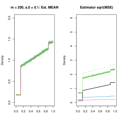
In this subsection we present the results of simulations studying the performance of our density estimators for estimating that has a piecewise continuous density on . In each simulation run we generate a sample of iid observations from and use it to compute for , and a set value of . As we estimate a dimensional density, we consider the canonical segmentation of , in which for and . We performed sets of simulations with and , each consisting of simulation runs.
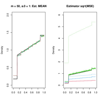
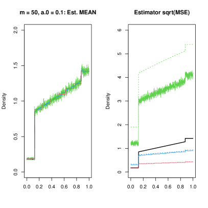
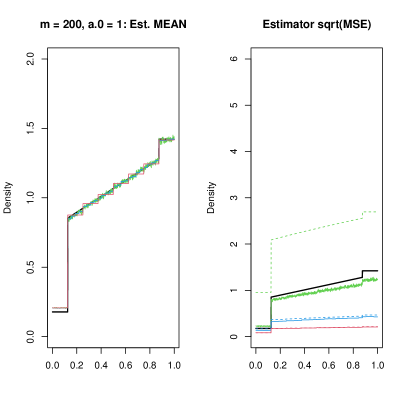
The simulation results are presented in Figure 4. Each pair of plots corresponds to the same set of simulations: the left plot displays the simulation mean of ; the right plot displays the square root of the simulation mean of the estimator squared-error, , for and for the interval-counts density estimators, . The black curve in all the plots is , the piecewise continuous density we are estimating. The green, blue, red curves correspond to level , segmentations of . Solid curves are drawn for the hBeta estimators and dashed curves are drawn for the interval-counts estimators.
The estimator mean plots reveal estimation bias and approximation error. For and the hBeta density estimators are biased – upward bias for small density values and downward bias for large density values. For and the bias of the estimators is smaller. For the bias is considerably smaller and can only be observed for the small density values. The bias does seem to depend on .
To assess approximation errors, which do not depend on and , we focus on the and configuration that has the smallest bias. There is no approximation error in the regions in which is constant. In the region in which is linear in , there is considerable approximation for that decreases as increases.
The estimator MSE is the sum of the squared estimation error and the squared approximation error. In this example the estimation error is considerably larger than the approximation error. The hBeta estimator MSE decreases in , and given and it increases in . For , and , the MSE of the hBeta estimator is the same as the MSE of the interval-counts estimator, which is unbiased with for all and . The ratio between the MSE of the interval-counts estimator and the hBeta estimator increases for larger and and smaller . For , and , the sqrt(MSE) of the hBeta estimator is times smaller than that of the interval-counts estimator.
3.2 Simulation study of 2D density estimation
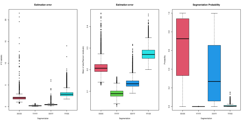
In this subsection, for , we present simulation results for estimating with , for the four level segmentations of shown in Figure 1.
The results are displayed in Figure 5. In the top row of plots we show how well is approximated by in the the four segmentations of . In each plot, the regions separated by the green vertical lines in each plot correspond to the subintervals of each segmentation, , arranged from left to right. Thus, in the four plots the last interval on the right is . According to Figure 1, for segmentation , is the subinterval on the right end of ; for segmentation , , is the subinterval on the top end of ; for segmentations and , is the subinterval on the top right corner of .
In the four plots, the black curves display the profile of as a function of and the red horizontal lines display , for each subinterval. We summarize the approximation error for each segmentation by the square root of a measuring the distance between and ,
Segmentation has the smallest approximation error, ; Segmentation has the largest approximation error, ; the approximation error for segmentations and , that have the same set level subintervals, is ;
The simulation study consisted of simulation runs. In each run, iid were generated and used to compute and the hBeta estimator, , for each segmentation with . The estimation error of is summarized by the Pearson residual, . Note that for each simulation run . Therefore Pearson residual for the counts estimator, , is approximately and the resulting statistic, which is the sum of squares of the Pearson residuals, is a chi-square random variable with degrees of freedom.
The boxplots in the bottom row of Figure 5 display the distribution of the simulation outcomes. The left and middle sets of boxplots display the distribution of and the distribution of the mean of the absolute value of the Pearson residuals, for the four segmentations. The plots reveal that the estimation error for all four segmentations is considerably smaller than the estimation error for the counts estimator, for which the expectation of the statistic is and the expectation of the mean of the absolute value of the Pearson residual is approximately . As our estimation algorithm shrinks the density at each level to the Uniform density, the estimation error is minimized for segmentation for which the estimated probabilities are equal, and increases as the differences in probabilities between contiguous subinterval increase. Thus even though the set of estimated probabilities is the same for segmentations and , the estimation error is much smaller for segmentation for which the set of probabilities is ordered.
The four boxplots on the right display the distribution of posterior segmentation probability for each segmentation. The plots reveal that that has the smallest approximation error is the most probable segmentation. Segmentation that has the largest approximation error has almost posterior probability. Of the two segmentations with the same approximation error, segmentation that has the smaller estimation error has considerably larger posterior probabilities.
4 Quantile regression simulation
In this simulated example is the density of , where for , and with for and for . We segment with dyadic segmentations. Similarly to the previous 2D example, we only consider in which all the subintervals at the same level are partitioned according to the same dimension. In this case is the set of segmentations consisting of four partitions and four partitions that produce an array of square subintervals, and we set .
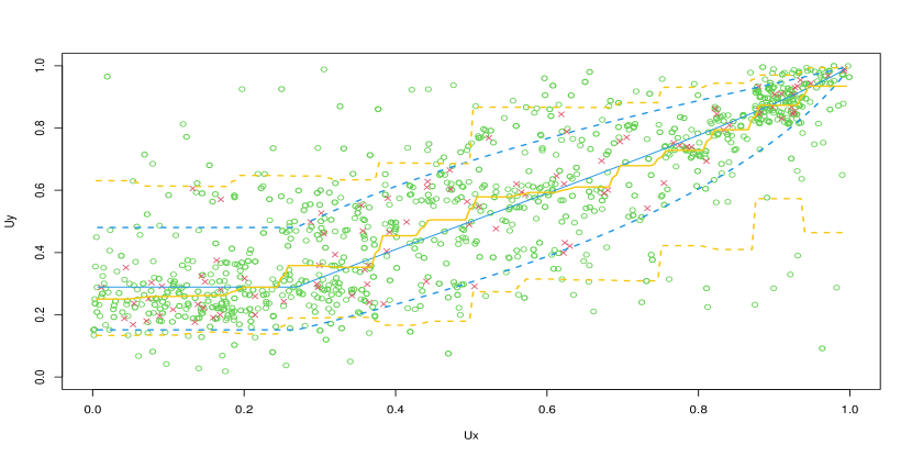
The plots in Figure 6 correspond to simulations with sample size (top) and (bottom). In each plot, the red X’s mark the observations, , and the blue curves are the , and quantiles of . Per construction, for all the interval between the dashed blue lines forms a conditional predictive interval for . Thus the region between the dashed blue lines is a predictive set for .
In order to produce predictive inferences, for each segmentation , we compute the posterior segmentation probability , and generate Beta vectors from the conditional distribution of given and and use them to compute probability vectors, . We approximate the posterior predictive density by the mixture density
| (16) |
The Green circles in each plot, are posterior predictive samples, , drawn independently from mixture density (16). The Orange curves are the , and quantiles of the conditional distribution of given for mixture density (16). Note that as the mixture density is piecewise constant on an array of subintervals, each quantile profile is piecewise constant on the subintervals of . For all the interval between the dashed Orange lines form a conditional posterior predictive interval for , thus the region between the dashed lines is a posterior credible prediction set.
The plots reveal that the posterior predictive density captures the general shape of pretty well. For , the conditional posterior predictive distribution is more spread out than , especially for values of close to , for which converges to . For , the distribution of the posterior predictive samples is more similar to the distribution of , and other than an approximation error, the quantiles of the conditional posterior predictive distribution and the quantiles of are almost the same for all .
4.1 Conformal Prediction sets
Vovk et al. (2005) present a general algorithm for constructing prediction sets for the following setting: are iid , with . On observing the training set and , the goal is to construct a prediction set for . The key component for constructing the prediction sets is the conformity score, , that shows how well an additional point conforms to the training set. They prove that Conformal Prediction Sets constructed in Algorithm 4.1 cover with probability .
Definition 4.1 Algorithm for constructing Conformal Prediction Sets
-
1.
For each potential value of , compute the conformity score
To assess the significance of , for compute conformity score
and compute the rank-based p-value
-
2.
The Conformal Prediction Set for is then defined
To construct conformal prediction sets for the quantile regression example, we define the conformity score between training set and an additional point to be the conditional posterior predictive given and that ,
| (17) |
To apply Algorithm 4.1, is conformity score (17) for and training set , which we numerically evaluate with mixture density (16). However for , is conformity score (17) for and training set , with . We evaluate by generating a mixture density (16) that approximates posterior predictive density .
Note that for the posterior predictive distribution identifies with , in which case the conformity score in (17) for is a random variable and thus the conformity score identifies with its significance level in Algorithm 4.1, . Thereby implying that the bottom end of the Conformal Prediction Set for is the quantile of the conditional posterior predictive distribution of .
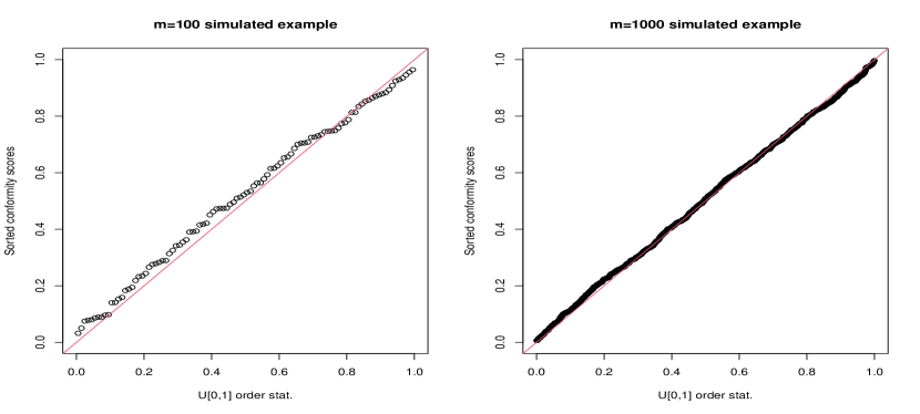
In the top row of Figure 7 we present qqplots for the sequence of conformity scores, between each of the observations and the training set consisting of the remaining observation, for the simulated examples shown in figure 6. For , we see that the distribution of the conformity scores for the observations is very close to . Thus the ends of the Conformal Prediction sets would be very close to the dashed orange curves in the bottom plot in Figure 6.
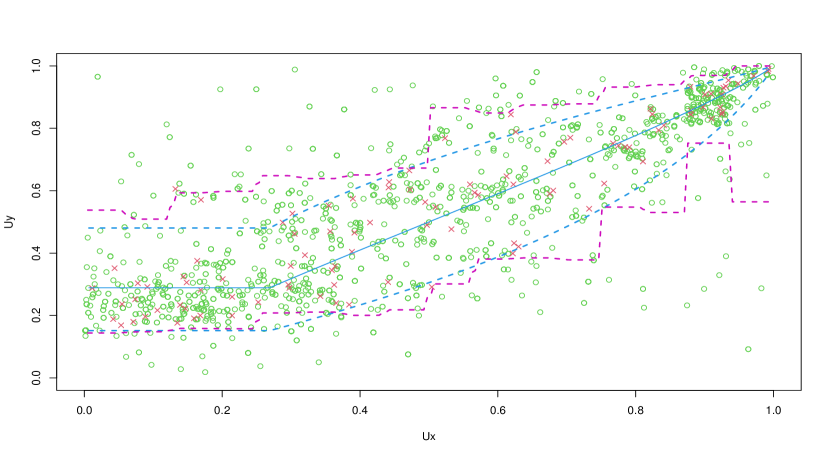
In the bottom of figure 7, we display the Conformal Prediction sets for the simulated example in Figure 6. The lower purple dashed curve marks the bottom ends of the Conformal Prediction Sets for for all , for conformity score . The upper purple dashed curve marks the top ends of the Conformal Prediction Sets for for all , for conformity score . Thus the region between the two purple curves forms a Conformal Prediction Set for .

5 High Dimensional Predictive Inference simulation
In this section, is the joint distribution of a categorical variable , which takes on values “a”, “b”, “c” with probabilities , , , and a continuous -dimensional random vector , with conditional distribution . and or all values of ; for or , ; for , , other than that .
In the simulated example, we generate iid realizations of , for . Our goal is to produce posterior predictive samples, .
To apply our methodology, for is transformed to as follows. For , the support of continuous variable is inflated by and partitioned into subintervals. For , let denote the quantile of . The marginal subintervals are then defined: , for , . For , we set for . Thus take on the values with probabilities . The categorical variable is encoded by two dichotomous variables: for and for ; for and for .
The sample is segmented with dyadic segmentations of , where for variable may be segmented times in halve and for variable may be segmented in halve once. is the set of segmentations, in which is first partitioned according to and and then according to either or – four partitions in each dimension – for all in . For the hBeta model we set .
For each segmentation , our method produces posterior predictive samples for variables, . As our model explicitly assumes a Uniform density within each segmentation, the values of the remaining continuous variables, for with and , is sampled with equal probabilities from . The posterior predictive sample, , is then generated by importance sampling on . Lastly, we produce the posterior predictive sample, as follows. if , if , otherwise . While, for and , is sampled from the Uniform distribution on subinterval , with .
Note that the normalizing transformation applied to the continuous variables, ensures that the marginal posterior predictive distribution of , , will be similar to the marginal distribution of even if is not included in . However, to ensure that the marginal posterior predictive distribution of will be similar to the marginal distribution of , variables and had to be included in each segmentation.
In Figure 8 we display the logarithm of numerator of Expression (2), which is proportional to the segmentation probability , for the segmentations in . The plot reveals that only the segmentations with continuous variables and had non-negligible selection probabilities. Thereby implying that the posterior predictive samples of were generated independently from a marginal distribution that is very similar to that of the original sample.
For all we set and , because according to our intuition beginning the segmentation with and is supposed to yield the largest segmentation probability. To test our intuition, , we compare the segmentation probability of to the segmentation probability of derived by setting for , , . And indeed, for all this change decreased the logarithm of the segmentation probabilities by more than .
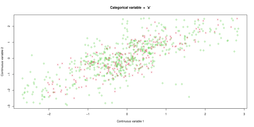
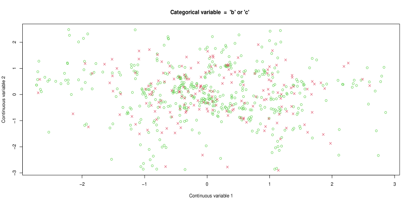
The sample of observations, , consisted of observations with , observations with , observations with . The posterior predictive sample of the categorical variable, , consisted of observations with , observations with , observations with . In Figure 9 we compare the joint conditional distribution of and , given and , for the original sample and for the posterior predictive sample. Figure 9 reveals that our method managed to pick up the relation between , and , in . While according to the results shown in Figure 8, our method also correctly modelled the independence in between , , and the other variables.

6 Discussion
We presented a Bayesian framework for density estimation and predictive inference that is based on multiple random dyadic segmentations of the P-dimensional unit cube. To apply our methodology to a sample of realizations of random vector , it is necessary to specify a mapping for each coordinate of into , set the value of and the segmentation level , and specify the set of segmentations .
Our working experience suggests setting . Our focus in this work is recovering the dependence between the components of . For small , a linear mapping between an interval, slightly larger than the support of , and should be satisfactory. For larger , the mapping we applied in Section 5, based on the empirical distribution of the variable, allowed us to recover the marginal distribution of a continuous variable without including it in the segmentation.
For the simulated examples, we considered segmentations in which all subintervals at the same level were partitioned according to the same coordinate (therefore was of order ) and we evaluated the posterior predictive distribution by importance sampling over all . This is not computationally feasible for large . To overcome this problem we plan to consider a richer family of segmentations , in which the subintervals in the same level may be partitioned in different directions, and to evaluate the posterior predictive distribution by MCMC algorithms that perform random walks on .
The most interesting property of our method, illustrated in the simulated examples, is that it favours segmentations for which the step-function density approximates the distribution of well, and yields a step-function density that is easy to estimate by a Polya tree. We plan to provide theoretical support for this observation, which we will try to formalize as conjectures. Note that each segmentation of into the level subintervals, , specifies a mapping from to (see Figure 1 and top row of plots in Figure 5). We conjecture that for which distribution is increasing with respect to this mapping have larger posterior probabilities; provide smaller approximation error; yield increasing step-function densities that are easier to estimate.
References
- [1] Ferguson, T. S. (1974) “Prior distributions on spaces of probability measures,” Annals of Statistics, 2, 615-629.
- [2] Ma, L. (2017) “Adaptive Shrinkage in Polya Tree Type Models”, Bayesian Analysis 12, 3,779-805.
- [3] Vovk, V., Gammerman, A., Shafer, G. (2005) “Algorithmic Learning in a Random World.” Springer.
- [4] Wong, W. H., Ma, L. (2010) “Optional Polya tree and Bayesian inference” Annals of Statistics, 38(3): 1433-1459.