A Global Optimization Approach for Multi-Marginal Optimal Transport Problems with Coulomb Cost

Abstract

In this work, we construct a novel numerical method for solving the multi-marginal optimal transport problems with Coulomb cost. This type of optimal transport problems arises in quantum physics and plays an important role in understanding the strongly correlated quantum systems. With a Monge-like ansatz, the orginal high-dimensional problems are transferred into mathematical programmings with generalized complementarity constraints, and thus the curse of dimensionality is surmounted. However, the latter ones are themselves hard to deal with from both theoretical and practical perspective. Moreover in the presence of nonconvexity, brute-force searching for global solutions becomes prohibitive as the problem size grows large. To this end, we propose a global optimization approach for solving the nonconvex optimization problems, by exploiting an efficient proximal block coordinate descent local solver and an initialization subroutine based on hierarchical grid refinements. We provide numerical simulations on some typical physical systems to show the efficiency of our approach. The results match well with both theoretical predictions and physical intuitions, and give the first visualization of optimal transport maps for some two dimensional systems.

49M37, 65K05, 81V05, 90C26, 90C30

1 Introduction

The aim of this paper is to provide an optimization method for the multi-marginal optimal transport (MMOT) problems [37, 44] arising in many-electron physics [11, 13, 42]. Let $d\in\{1,2,3\}$ be the dimension of system, $\Omega\subseteq\mathbb{R}^{d}$ be a bounded domain where the electrons are located, $N\in\mathbb{N}$ with $N\geq 2$ be the number of electrons and $\boldsymbol{r}_{i}\in\Omega~{}(i\in\{1,\ldots,N\})$ be the position of the $i$-th electron. For the many-electron system, the MMOT problem with Coulomb cost reads

(1) $$\begin{array}[]{cl}\displaystyle\min_{\gamma}&\displaystyle\int_{\Omega^{N}}c\big{(}\boldsymbol{r}_{1},\ldots,\boldsymbol{r}_{N}\big{)}\gamma\big{(}\boldsymbol{r}_{1},\ldots,\boldsymbol{r}_{N}\big{)}~{}{\rm d}\boldsymbol{r}_{1}\cdots~{}{\rm d}\boldsymbol{r}_{N}\\ \displaystyle\text{subject to}~{}(\mathrm{s.}~{}\mathrm{t.})&\displaystyle\Pi_{i}\gamma(\boldsymbol{r})=\frac{1}{N}\rho(\boldsymbol{r}),\quad i=1,\ldots,N,\quad\forall~{}\boldsymbol{r}\in\Omega,\end{array}$$

where the cost function $c\big{(}\boldsymbol{r}_{1},\ldots,\boldsymbol{r}_{N}\big{)}$ is determined by the electron-electron Coulomb interaction

(2) $$c\big{(}\boldsymbol{r}_{1},\ldots,\boldsymbol{r}_{N}\big{)}:=\sum_{i<j}\frac{1}{|\boldsymbol{r}_{i}-\boldsymbol{r}_{j}|},$$

$\gamma\big{(}\boldsymbol{r}_{1},\ldots,\boldsymbol{r}_{N}\big{)}$ is an $N$-point probability measure on $\Omega^{N}$, with the single-electron density $\rho:\Omega\to\mathbb{R}$ being the $i$-th marginal $\Pi_{i}\gamma$, i.e. for any $\boldsymbol{r}\in\Omega$, $\frac{1}{N}\rho(\boldsymbol{r})$ equals

(3) $$\Pi_{i}\gamma(\boldsymbol{r}):=\int_{\Omega^{N-1}}\gamma\big{(}\boldsymbol{r}_{1},\ldots,\boldsymbol{r}_{i-1},\boldsymbol{r},\boldsymbol{r}_{i+1},\ldots,\boldsymbol{r}_{N}\big{)}~{}{\rm d}\boldsymbol{r}_{1}\cdots~{}{\rm d}\boldsymbol{r}_{i-1}~{}{\rm d}\boldsymbol{r}_{i+1}\cdots~{}{\rm d}\boldsymbol{r}_{N}.$$

Note that the Coulomb interaction $1/|\boldsymbol{r}_{i}-\boldsymbol{r}_{j}|$ between the electrons in (2) can be approximated or regularized, especially in the simulations of systems with $d<3$ [4, 19]. Nevertheless, the approach constructed in this paper will make no essential difference as long as the interaction between the electrons is repulsive (i.e. the cost decreases with respect to $|\boldsymbol{r}_{i}-\boldsymbol{r}_{j}|$). Therefore in this paper, we will focus ourselves on the Coulomb interaction of the form (2).

The MMOT problem Eq. 1 with Coulomb cost Eq. 2 arises as the strictly correlated electrons limit in the density functional theory (DFT). DFT has been most widely used for electronic structure calculations in physics, chemistry, and material sciences (see [3] for a review). The strictly correlated electrons limit was first introduced in [41], later noticed in [7, 12] that the limit problem is an optimal transport problem. The strictly correlated electrons limit provides an alternative route to derive the DFT energy functionals and has been exploited to extend the capability of DFT to treat strongly correlated quantum systems [9, 10, 21, 32, 34].

Direct discretization of the MMOT problem Eq. 1 leads to a linear programming, with the size increasing exponentially fast with respect to $N$ (the number of electrons/marginals). There are several works devoted to numerical methods that try to circumvent the curse of dimensionality. In [5], the Sinkhorn scaling algorithm based on iterative Bregman projections was applied to an entropy-regularized discretized MMOT problem of 1D systems. In [7, 33], the numerical methods based on Kantorovich dual of the MMOT problem were proposed, while there are exponentially many constraints in the dual problem. In [29, 30], a convex relaxation approach was proposed by imposing certain necessary constraints satisfied by the two-marginal, and the relaxed problem was then solved by semidefinite programming to obtain tight lower bounds for the optimal cost. In [1, 2], the existence of sparse global solutions was established and a constrained overdamped Langevin process was proposed to solve the moment constrained relaxations. In [19, 20], the sparsity of optimal solution was rigorously justified and an efficient numerical method was proposed based on column generation and machine learning.

The starting point of this work is to approximate the $N$-point measure $\gamma$ by the following ansatz

(4) $$\gamma(\boldsymbol{r}_{1},\ldots,\boldsymbol{r}_{N})=\frac{\rho(\boldsymbol{r}_{1})}{N}\gamma_{2}(\boldsymbol{r}_{1},\boldsymbol{r}_{2})\cdots\gamma_{N}(\boldsymbol{r}_{1},\boldsymbol{r}_{N}),$$

where $\gamma_{i}:\Omega^{2}\to\mathbb{R}~{}(i\in\{2,\ldots,N\})$ satisfies

(5) $$\gamma_{i}(\boldsymbol{r},\boldsymbol{r}^{\prime})\geq 0,\quad\int_{\Omega}\gamma_{i}(\boldsymbol{r},\boldsymbol{r}^{\prime})~{}{\rm d}\boldsymbol{r}^{\prime}=1,\quad{\rm and}\quad\int_{\Omega}\rho(\boldsymbol{r})\gamma_{i}(\boldsymbol{r},\boldsymbol{r}^{\prime})~{}{\rm d}\boldsymbol{r}=\rho(\boldsymbol{r}^{\prime}).$$

Here we do not have $\gamma_{1}$ since $\gamma_{1}(\boldsymbol{r},\boldsymbol{r}^{\prime})=\theta(\boldsymbol{r}-\boldsymbol{r}^{\prime})$ by convention, where $\theta$ is the Dirac delta function. The condition Eq. 5 is derived from the multi-marginal constraints Eq. 3. From a physical point of view, $\gamma_{i}(\boldsymbol{r},\boldsymbol{r}^{\prime})$ represents the correlation between the first and the $i$-th electron, which gives the probability of finding the $i$-th electron at $\boldsymbol{r}^{\prime}$ while the first electron is located at $\boldsymbol{r}$. Under ansatz Eq. 4, the MMOT problem Eq. 1 (with $N>2$) can be rewritten as

(6) $$\min_{\gamma_{2},\ldots,\gamma_{N}}\left\{\sum_{2\leq i<j\leq N}\int_{\Omega}\int_{\Omega}\int_{\Omega}\frac{\rho(\boldsymbol{r})\gamma_{i}(\boldsymbol{r},\boldsymbol{r}^{\prime})\gamma_{j}(\boldsymbol{r},\boldsymbol{r}^{\prime\prime})}{|\boldsymbol{r}^{\prime}-\boldsymbol{r}^{\prime\prime}|}~{}{\rm d}\boldsymbol{r}~{}{\rm d}\boldsymbol{r}^{\prime}~{}{\rm d}\boldsymbol{r}^{\prime\prime}\right.\\ \left.+\sum_{2\leq i\leq N}\int_{\Omega}\int_{\Omega}\frac{\rho(\boldsymbol{r})\gamma_{i}(\boldsymbol{r},\boldsymbol{r}^{\prime})}{|\boldsymbol{r}-\boldsymbol{r}^{\prime}|}~{}{\rm d}\boldsymbol{r}~{}{\rm d}\boldsymbol{r}^{\prime}~{}:~{}\gamma_{2},\ldots,\gamma_{N}~{}{\rm satisfy}~{}\lx@cref{creftype~refnum}{conditions:gammas}\right\}.$$

We mention that in the case of $N=2$, the first term in the objective of (6) vanishes, then the problem is reduced to a linear programming and can be solved by standard algorithms [10]. In this work, we focus our attention on the $N\geq 3$ settings. The formulation Eq. 6 amounts to a spectacular dimension reduction, in that the unknowns are $N-1$ transports on $\Omega^{2}$ instead of the $N$-point measure $\gamma$ on $\Omega^{N}$. Therefore, the degrees of freedom now scale linearly with respect to $N$ rather than exponentially fast. In particular, the ansatz Eq. 4 includes the Monge state [35, 42] by taking $\gamma_{i}(\boldsymbol{r},\boldsymbol{r}^{\prime})=\theta\big{(}\boldsymbol{r}^{\prime}-T_{i}(\boldsymbol{r})\big{)}$ with $T_{i}~{}(i\in\{2,\ldots,N\})$ being the so-called optimal transport map. The Monge formulation gives significant information on the MMOT problem and enjoys physical interpretations; see more discussions in Section 1.3.

In practical calculations, we need to discretize Eq. 6 into some finite dimensional problems. The discretization consists of three steps. First, we employ a finite elements like mesh $\mathcal{T}=\left\{e_{k}\right\}_{k=1}^{K}$ to partition the domain $\Omega$ into $K$ non-overlapping elements, i.e. $\bigcup_{k=1}^{K}e_{k}=\Omega$ and $e_{i}\bigcap e_{j}=\emptyset$ when $i\neq j$. Let $e:=[\left|e_{1}\right|,\ldots,\left|e_{K}\right|]^{\top}\in\mathbb{R}_{+}^{K}$ denote the volumes of elements. Second, we approximate the marginal $\rho$ by a vector $\varrho:=[\varrho_{1},\ldots,\varrho_{K}]^{\top}\in\mathbb{R}_{+}^{K}$, where the $k$-th entry $\varrho_{k}:=\frac{1}{\left|e_{k}\right|}\int_{e_{k}}\rho(\boldsymbol{r})~{}{\rm d}\boldsymbol{r}$ gives the marginal/electron mass on the $k$-th element $e_{k}$. Finally, the Coulomb interactions and and the transports $\gamma_{i}~{}(i=2,\cdots,N)$ can be approximated by the effective interactions and transports between elements, i.e. for any $j,k\in\{1,\ldots,K\}$,

(7) $$c_{jk}:=\frac{1}{\left|e_{j}\right|\cdot\left|e_{k}\right|}\int_{e_{k}}\int_{e_{j}}\frac{1}{\left|\boldsymbol{r}-\boldsymbol{r}^{\prime}\right|}~{}{\rm d}\boldsymbol{r}~{}{\rm d}\boldsymbol{r}^{\prime}\quad\text{and}\quad x_{i,jk}:=\frac{1}{\left|e_{j}\right|\cdot\left|e_{k}\right|}\int_{e_{k}}\int_{e_{j}}\gamma_{i}(\boldsymbol{r},\boldsymbol{r}^{\prime})~{}{\rm d}\boldsymbol{r}~{}{\rm d}\boldsymbol{r}^{\prime},$$

respectively, leading to $K\times K$ matrices $C:=((1-a_{jk})c_{jk})_{jk}$ and $X_{i}=(x_{i,jk})_{jk}$ for $i=2,\ldots,N$. Here $a_{jk}$ equals $1$ if $j=k$ and $0$ otherwise. With this discretization, we can approximate Eq. 6 using the following optimization problem with unknowns $\{X_{i}\}_{i=2}^{N}$:

(8) $$\begin{array}[]{cl}\displaystyle\min_{X_{2},\ldots,X_{N}}&\displaystyle f(X_{2},\ldots,X_{N}):=\sum_{2\leq i\leq N}\left\langle X_{i},\Lambda\Xi C\Xi\right\rangle+\sum_{2\leq i<j\leq N}\left\langle X_{i},\Xi\Lambda X_{j}\Xi C\Xi\right\rangle\\ \mathrm{s.}~{}\mathrm{t.}&X_{i}e=\mathbf{1},~{}X_{i}^{\top}\Xi\varrho=\varrho,~{}\mathrm{Tr}(X_{i})=0,~{}X_{i}\geq 0,~{}i=2,\ldots,N,\\ &\left\langle X_{i},X_{j}\right\rangle=0,~{}\forall~{}i\neq j,\end{array}$$

where $\mathbf{1}$ is the all-one vector in $\mathbb{R}^{K}$, $\Lambda=\mathrm{Diag}(\varrho),~{}\Xi=\mathrm{Diag}(e)$ are $K\times K$ diagonal matrices formed by entries in $\varrho$ and $e$, respectively. More detailed derivation of Eq. 8 is given in Appendix A. Note that the diagonal elements in matrix $C$ are removed due to integral divergence in Eq. 7. The extra constraints

$$\mathrm{Tr}(X_{i})=0,~{}i=2,\ldots,N,\quad\text{and}\quad\left\langle X_{i},X_{j}\right\rangle=0,~{}\forall~{}i\neq j$$

are hence accordingly added. From a physical point of view, this constraint can keep the electrons spatially away from each other in the case of Coulomb repulsion, so that unfavorable particle clustering can be avoided.

In the case of $N=3$, Eq. 8 is a mathematical programming with complementarity constraints (MPCC) in view of nonnegative constraints and $\left\langle X_{2},X_{3}\right\rangle=0$. Due to the disjunctive nature of feasible set, a general MPCC violates commonly used constraint qualifications at any feasible point [15]. As a result, the well-known Karush-Kuhn-Tucker conditions are no longer certificate for feasible points to be local minimizers. When $N>3$, the formulation of the constraints in Eq. 8 is more complicated than that of the complementarity constraints. Since $\left\langle X_{i},X_{j}\right\rangle,~{}\forall~{}i\neq j$ impose the requirements that, for each $i\in\{2,\ldots,N\}$, the block variable $X_{i}$ complements all the other blocks, we call Eq. 8 a mathematical programming with generalized complementarity constraints (MPGCC).

In addition to its intrinsic difficulty, we are in quest for global solutions of Eq. 8. This is a hard matter because both the repulsive energy $f$ and the feasible set are nonconvex in variables $(X_{i})_{i=2}^{N}$. Since the degrees of freedom $(N-1)K^{2}$ grow quickly as the meshes become finer, the state-of-art global optimization solvers cannot be our last resort.

1.1 Optimization Background

Although little is known about MPGCC, there exists rich literature on MPCC. To overcome the intrinsic difficulties mentioned above, several MPCC-tailored constraint qualifications have been provided for MPCC. Under these constraint qualifications, points satisfying certain stationary systems are shown to be proper candidates of local minimizers. The related notions and theoretical results are gathered in [38, 47] and the references within.

With these in place, researchers have proposed various numerical approaches, wherein those based on the original MPCC formulation rank top choices; they employ the modified nonlinear programming solvers. For example, the authors in [17] solved MPCCs using sequential quadratic programming algorithm with filter techniques [16]; the software introduced in [8, 45] incorporates a suite of nonlinear programming algorithms to tackle MPCCs, including interior-point methods and sequential quadratic programming algorithm, together with globalization techniques such as line search and trust region.

Owing to the troubles when coping with complementarity constraints, methods based on penalty functions gain popularity as well. Among others, we confine our attention to the $\ell_{1}$ (complementarity) penalty function, which favours direct extension to MPGCC Eq. 8 as

(9) $$f(X_{2},\ldots,X_{N})+\beta\sum_{i<j}\left\langle X_{i},X_{j}\right\rangle,$$

namely, penalizing merely the complementarity violation in $\ell_{1}$ form. Here $f$ is the repulsive energy defined in Eq. 8, $\beta>0$ is the penalty parameter. Apart from algorithmic benefit, with $N=3$, it can be verified under certain conditions that the global solutions of Eq. 8 coincide with those globally minimizing Eq. 9 over $\mathcal{S}^{N-1}$, where

(10) $$\mathcal{S}:=\{W\in\mathbb{R}^{K\times K}:We=\mathbf{1},~{}W^{\top}\Xi\varrho=\varrho,~{}\mathrm{Tr}(W)=0,~{}W\geq 0\}.$$

A direct consequence is that, if the global solutions of Eq. 8 are required, one can in turn minimize Eq. 9 over $\mathcal{S}^{N-1}$ starting with proper initialization. However, we are not aware of any existing method that fully exploits the special structure of (9). A customized algorithm is thus needed, particularly in the large-scale context.

In addition, methods based on approximation (smoothing or regularization), augmented Lagrangian functions and full penalization are available as well. We refer interested readers to [14, 25, 26, 27, 39, 40] and the references therein. Compared with methods using modified nonlinear programming solvers or penalty functions, other approaches suffer from an obvious drawback: for a specific MPGCC, the latter ones require solving a sequence of subproblems in the same size to stationarity or even optimality [28]. This weakness excludes them from our choices, particularly when the number of grid points $K$ is tremendously large.

1.2 Contributions

Our contributions are three-fold:

1. A global optimization approach, equipped with a local solver and a hierarchical initialization subroutine, is constructed for solving Eq. 8.

   The initialization subroutine (Algorithm 2), derived from hierarchical grid refinements, helps the local solver locate good approximations of global solutions, and hence serves as the core of the proposed global optimization approach (Framework 1). The proposed approach saves one from brute-force solving large-scale Eq. 8 via plain global optimization methods. Remarkably in Framework 1, the optimal transport maps can be directly evaluated by the solutions, which is usually difficult in the context of Coulomb cost.

2. An inexact proximal block coordinate descent (PBCD) algorithm is proposed for locally minimizing Eq. 9 over $\mathcal{S}^{N-1}$.

   The PBCD algorithm (Algorithm 3) acts as the local solver in Framework 1 and enjoys global convergence guarantee in the presence of iterate infeasibility (Theorem 3.2), which is not covered by existing works.

3. Simulations of optimal transport maps for some typical 1D and 2D systems.

   We consider systems with the number of electrons up to 7, and discretization with the number of grid points up to $1.6\times 10^{4}$. The results are in line with both theoretical predictions and physical intuitions (Section 4). We also give the first visualization of optimal transport maps for some 2D systems.

1.3 Further Remarks

Monge formulations. It is unknown whether the MMOT problem Eq. 1 with Coulomb cost has a solution of the form Eq. 4. However, the ansatz Eq. 4 includes the Monge solutions, which are most widely studied in physics. The Monge formulation makes the ansatz

(11) $$\gamma(\boldsymbol{r}_{1},\ldots,\boldsymbol{r}_{N})=\frac{\rho(\boldsymbol{r}_{1})}{N}\theta\left(\boldsymbol{r}_{2}-T_{2}(\boldsymbol{r}_{1})\right)\cdots\theta\left(\boldsymbol{r}_{N}-T_{N}(\boldsymbol{r}_{1})\right),$$

where $\theta$ is the Dirac delta function, the transport map $T_{i}:\Omega\to\Omega~{}(i\in\{2,\ldots,N\})$ (we can prescribe $T_{1}(\boldsymbol{r})=\boldsymbol{r}$ for completeness of notations) preserves the single-electron density $\rho$. The Monge solution has a simple physical interpretation: the many-electron repulsive energy is minimized at a state such that one electron at position $\boldsymbol{r}$ can determine the positions of all other $N-1$ electrons via $\{T_{i}\}_{i=2}^{N}$. It is known that for 1D systems, the Monge formulation gives the global solution of the MMOT problems [11, 12]. But in the general $d>1$ and $N>2$ cases, it is unknown whether there exists a minimizer of Eq. 1 in the form Eq. 4. Nevertheless, the Monge solution involves a lot of physical information of the many-electron system and can give rise to the Kantorovich potential (which is needed in applications for electronic structure); see [42, 43]. Therefore, the Monge solution is crucial for the MMOT problems in DFT, which is though still difficult to evaluate in the context of Coulomb cost. In our Framework 1, however, the optimal transport maps $\{T_{i}\}_{i=2}^{N}$ can be approximated by the transportation between elements in mesh. More precisely, let $\boldsymbol{a}_{j}$ be the barycenter of the element $e_{j}$, then $T_{i}(\boldsymbol{a}_{j})~{}(i=2,\cdots,N)$ can be approximated by solution $(X_{i})_{i=2}^{N}$ as

(12) $$T_{i}^{K}(\boldsymbol{a}_{j}):=\frac{\sum_{1\leq k\leq K}\boldsymbol{a}_{k}x_{i,jk}}{\sum_{1\leq l\leq K}x_{i,jl}},\quad j=1,\ldots,K,\quad i=2,\ldots,N.$$

Symmetric constraints. In physics, one is only interested in the measures that are symmetric with respect to $\{\boldsymbol{r}_{i}\}$ (as $\gamma(\boldsymbol{r}_{1},\ldots,\boldsymbol{r}_{N})$ represents $N$-point position density of electrons, which is symmetric by the laws of quantum theory). More precisely, one requires that for any permutation $\mathscr{P}$ on $\{1,\ldots,N\}$, $\gamma\big{(}\boldsymbol{r}_{1},\ldots,\boldsymbol{r}_{N}\big{)}=\gamma\big{(}\boldsymbol{r}_{\mathscr{P}(1)},\ldots,\boldsymbol{r}_{\mathscr{P}(N)}\big{)}$. Although we do not have this symmetric restriction in the MMOT problem Eq. 1 and the ansatz Eq. 11 is in general not symmetric, dropping the restriction does not alter the minimum value. This is because we have a symmetric cost function $c$ in Eq. 2 and equal marginal for any $\Pi_{i}\gamma$ in Eq. 3. Hence each non-symmetric $\gamma$ can give a symmetric one with the same energy value by symmetrization $\frac{1}{N!}\sum_{\mathscr{P}}\gamma\big{(}\boldsymbol{r}_{\mathscr{P}(1)},\ldots,\boldsymbol{r}_{\mathscr{P}(N)}\big{)}$. We do not have to impose the symmetric constraints in the optimization formulation Eq. 8.

Discretization. Most of the existing works discretize the MMOT problems with real space methods [5, 10]. Particularly, this paper discretizes Eq. 6 into Eq. 8 by representing the marginal $\rho$ with piecewise finite elements and using effective cost coefficients obtained by integrating the continuous cost functions with respect to these elements. To further reduce the computational cost (i.e. use less grid points where the marginal is small), we choose the elements adaptively such that each element carries approximately the same marginal mass.

1.4 Outline

The rest of this paper is organized as follows. We introduce the global optimization approach in Section 2, where the initialization subroutine (Section 2.1) and the local solver (Section 2.2) are detailed in order. Section 3 is dedicated to the rough statements of the convergence property of PBCD. We corroborate the proposed approach with numerical simulations on several typical systems in Section 4. Finally, conclusions and discussions are drawn in Section 5.

1.5 Notations

The image of a linear operator $\mathcal{A}$ is denoted by $\mathrm{Im}(\mathcal{A})$. The notation $\|X\|_{p}$ gives the $p$-norm of matrix $X$, while $\|X\|_{\mathrm{F}}$ yields its Frobenius norm. The components of matrices or vectors are indicated by subscripts, e.g. $x_{ij}$. The inquality $X\geq 0$ means $x_{ij}\geq 0,~{}\forall~{}i,j$.

The notation $\delta_{S}$ represents the indicator function of set $S$, namely $\delta_{S}(x)$ equals $0$ if $x\in S$ otherwise $\infty$. For the multi-block objective functions referred in this work (such as Eq. 8), we occasionally adopt abbreviations in brackets. For example, $f(X_{<i},X_{i},X_{>i})$ means $f(X_{2},\ldots,X_{i-1},X_{i},X_{i+1},\ldots,X_{N})$; abbreviations like $X_{<i}$, $X_{(i,j)},X_{>j}$ represent aggregation of blocks with certain subscripts.

Regarding algorithm, we use (double) superscripts within bracket for iterates in outer (inner) loop; for instance, $X^{(l)}$ is the iterate in the $l$-th outer iteration, $X^{(l,k)}$ is the iterate in the $k$-th inner iteration of the $(l+1)$-th outer iteration.

2 A Global Optimization Approach for Solving (8)

In light of ansatz Eq. 4, the original MMOT problem with Coulomb cost Eq. 1 is approximated by MPGCC Eq. 8. Violating commonly used constraint qualifications, MPGCC Eq. 8 itself is a hard nut to crack from both algorithmic design and theoretical analysis. Rather, we concentrate on the $\ell_{1}$ penalized MPGCC Eq. 8, i.e.

(13) $$\begin{array}[]{cl}\displaystyle\min_{X_{2},\ldots,X_{N}}&\displaystyle f_{\beta}(X_{2},\ldots,X_{N}):=f(X_{2},\ldots,X_{N})+\beta\sum_{i<j}\left\langle X_{i},X_{j}\right\rangle\\ \mathrm{s.}~{}\mathrm{t.}&X_{i}\in\mathcal{S},~{}i=2,\ldots,N,\end{array}$$

where $f$ is the repulsive energy defined in Eq. 8, $\mathcal{S}$, defined in Eq. 10, stands for a section of feasible region. Problem Eq. 13 is a nonconvex quadratic programming problem, still NP-hard [36]. In the sequel, when we reference Eq. 13 and its solution in space $\big{(}\mathbb{R}^{K\times K}\big{)}^{N-1}$, we simply say Eq. 13 and its solution with size $K$.

For practical purposes, a global solution of Eq. 13 is always required. Meanwhile, we notice that the degrees of freedom in Eq. 13, $(N-1)K^{2}$, grow fast w.r.t. $K$. This prevents us from brute-force solving Eq. 13 by state-of-art global optimization methods (e.g. branch-and-bound and cutting plane algorithm) due to exponentially increasing running time.

Motivated by [5], we propose a global optimization approach GGR; see Framework 1.

Framework 1 The GGR approach

0:  Oracle returning $R,e,\varrho$ in proper dimensions; global solver; local solver; the GR subroutine; initial mesh with $K^{(0)}$ elements $\{e^{(0)}_{j}\}$.

1:  Set $l:=0$.

2:  GGR_Init: use global solver to solve Eq. 13 with size $K^{(0)}$ and get $(X_{i}^{(0)})_{i=2}^{N}$.

3:  while certain stopping criteria are not satisfied do

4:     Refine the last mesh $\{e^{(l)}_{j}\}$ to $\{e^{(l+1)}_{j}\}$ with $K^{(l+1)}$ elements.

5:     Modify $(X_{i}^{(l)})_{i=2}^{N}$ using the GR subroutine to obtain $(X_{i}^{(l,0)})_{i=2}^{N}$.

6:     GGR_LS$(l+1)$: start local solver from $(X_{i}^{(l,0)})_{i=2}^{N}$ to solve Eq. 13 with size $K^{(l+1)}$ and get $(X_{i}^{(l+1)})_{i=2}^{N}$.

7:     $l:=l+1$.

8:  end while

9:  return  $(X_{i}^{(l)})_{i=2}^{N}\in\big{(}\mathbb{R}^{K^{(l)}\times K^{(l)}}\big{)}^{N-1}$.

Here, “G” and “GR” stand for global optimization and the GR initialization subroutine based on hierarchical grid refinement, respectively. GGR_Init and GGR_LS are in turn referred to as the initial step invoking a global solver, and the subsequent step invoking a local solver. Framework 1 progresses step by step along with the process of mesh refinements.

Justification on the usage of global solver in the initial step (2 in Framework 1) is in order. From the point of applicability, given initial size $K^{(0)}$ of moderate magnitude, globally solving Eq. 13 is amenable to state-of-art global optimization methods. Considering the necessity, the quality of constructed initial points largely depends on the solutions in the previous step. Hence it is a natural choice for us to invoke a global solver in the initial step. For our choices in implementation, please refer to Section 4.1.

Without specification, the mesh refinements (4 in Framework 1) are done such that the coarse meshes are always embedded into the refined meshes. For more remarks, see Section 1.3. Although the refinements are uniform in the numerical simulations of present work (Sections 4.2 and 4.3), practical implementations focus on the region where marginals vary violently. Nevertheless in the latter circumstances, our GGR approach still works.

In what follows, we leave the initialization subroutine part to Section 2.1 and the local solver part to Section 2.2, respectively.

2.1 Initialization Subroutine based on Grid Refinement

Brute-force global optimization of Eq. 13 becomes impracticable once $K$ grows large. One treatment for this is arming a local solver with good initialization. Roughly speaking, if the energy surface forms a basin around the global solution $(X_{i})_{i=2}^{N}$, the local solver is able to find $(X_{i})_{i=2}^{N}$ provided the initial point lies inside the basin near $(X_{i})_{i=2}^{N}$. This subsection is devoted to the development of the GR subroutine for initialization (5 in Framework 1). In words, the GR subroutine passes the solution information of previous step on to the current one such that good initialization can be anticipated. Without this process, the located point by local solver is very likely not a global minimizer, resulting in bad solution afterwards.

We derive the GR subroutine from some 1D numerical experience: for a particular problem (given oracle of $R,e,\varrho$), the solutions with different sizes share “similar” patterns. This phenomenon suggests that we can construct an initial point based on the pattern reflected in the solution with a small size $K$. This point was also observed in [5], where the authors supplied a refinement strategy to meet the accuracy demand with relatively low cost for discretized 1D Eq. 1. Their strategy, however, remains to be explained rigorously and quantitatively. More importantly, they did not discuss the treatment in higher-dimensional context. In the following, we try to understand the “similarity” standing at optimal transport and then introduce the GR subroutine. Basically, the proposed subroutine is applicable under any space dimension $d$.

Let us begin with 1D setting. Suppose we already have a finite elements mesh $\{e_{j}\}$ and a global solution $(X_{i})_{i=2}^{N}$ of Eq. 13 with $X_{i}=(x_{i,jk})_{jk}$. Then for any $i\in\{2,\ldots,N\}$, $x_{i,jk}>0$ means that mass of $x_{i,jk}$ is transported from $e_{j}$ to $e_{k}$ by transport $X_{i}$. For the problem with a doubly refined mesh $\{\tilde{e}_{k}\}$, the original $e_{j},e_{k}$ correspond to $\tilde{e}_{2j-1}$ and $\tilde{e}_{2j}$, $\tilde{e}_{2k-1}$ and $\tilde{e}_{2k}$, respectively. Let $j_{1}=2j-1,~{}j_{2}=2j,~{}k_{1}=2k-1,~{}k_{2}=2k$. A reasonable speculation is that there also exists certain mass transported from $\tilde{e}_{2j-1},\tilde{e}_{2j}$ to $\tilde{e}_{2k-1},\tilde{e}_{2k}$ by the new $\widetilde{X}_{i}=(\tilde{x}_{i,mn})_{mn}$, i.e. $\tilde{x}_{i,j_{t}k_{u}}>0$, $t,u\in\{1,2\}$, which happens to explain the similarity observed in [5]. See Figure 1 for illustration.

Figure 1: 1D case. The red block means there is mass transported from 3 to 4. Then in a doubly refined mesh, there is mass transported from 5 and 6 to 7 and 8, as is marked out by 4 blue blocks.

The above reasoning applies to any $d\in\mathbb{N}$. Suppose a finite elements mesh $\{e_{j}\}$ and a global solution $(X_{i})_{i=2}^{N}$ are at hand, with $X_{i}=(x_{i,jk})_{jk}$. Then for any $i\in\{2,\ldots,N\}$, $x_{i,jk}>0$ means that mass of $x_{i,jk}$ is transported from element $e_{j}$ to $e_{k}$ by transport $X_{i}$. After mesh refinement, the original $\{e_{j}\}$ becomes $\{\tilde{e}_{k}\}$; for each $j$, the original element $e_{j}$ is divided into $s_{j}$ parts: $e_{j}=\bigcup_{t=1}^{s_{j}}\tilde{e}_{j_{t}}$ and $\tilde{e}_{j_{t_{1}}}\bigcap\tilde{e}_{j_{t_{2}}}=\emptyset$ when $j_{t_{1}}\neq j_{t_{2}}$. A reasonable speculation is that there also exists certain mass transported from $\tilde{e}_{j_{t}}$ to $\tilde{e}_{k_{u}}$, where $t\in\{1,\ldots,s_{j}\},~{}u\in\{1,\ldots,s_{k}\}$. Accordingly in $\tilde{X}_{i}=(\tilde{x}_{i,mn})_{mn}$, there should be $\tilde{x}_{i,j_{t}k_{u}}>0$, $s_{j}\times s_{k}$ positive entries in total. We make illustration for 2D case in Figure 2. Note that the coordinates in transport are rearranged from the 2D coordinates in mesh.

Figure 2: 2D case ($7\times 7$ rectangular mesh). The red block means there is mass transported from (1,5) to (2,4). Then in a doubly refined mesh, there is mass transported from (1,9), (1,10), (2,9) and (2,10) to (3,7), (3,8), (4,7) and (4,8), as is marked out by 16 blue blocks.

Based upon the above arguments, we derive the GR subroutine for initialization; see Algorithm 2.

Algorithm 2 The GR initialization subroutine

0:  Coarse mesh with $K$ elements $\{e_{j}\}$ and refined mesh with $\tilde{K}$ elements $\{\tilde{e}_{k}\}$; Solution of the previous step $(X_{i})_{i=2}^{N}$; scaling factor $r>0$.

1:  for $i=2,\ldots,N$ do

2:     for $j=1,\ldots,K$ do

3:        for $k=1,\ldots,K$ do

4:           if $x_{i,jk}>0$ then

5:              Find $\tilde{e}_{j_{t}},~{}t=1,\ldots,s_{j}$ such that $e_{j}=\bigcup_{t=1}^{s_{j}}\tilde{e}_{j_{t}}$.

6:              Find $\tilde{e}_{k_{u}},~{}u=1,\ldots,s_{k}$ such that $e_{k}=\bigcup_{u=1}^{s_{k}}\tilde{e}_{k_{u}}$.

7:              Set $\tilde{x}_{i,j_{t},k_{u}}=r\cdot x_{i,jk}$ for $t\in\{1,\ldots,s_{j}\},~{}u\in\{1,\ldots,s_{k}\}$.

8:           end if

9:        end for

10:     end for

11:  end for

12:  return  $(\tilde{X}_{i})_{i=2}^{N}\in\big{(}\mathbb{R}^{\tilde{K}\times\tilde{K}}\big{)}^{N-1}$, where for any $i$, $\tilde{X}_{i}=(\tilde{x}_{i,mn})_{mn}$.

2.2 Local Solver

The global solver and the GR subroutine make brute-force globally solving large-scale Eq. 13 unnecessary. Instead, we only need to provide a local solver (see 6 in Framework 1). We assume the procedure is in the $(l+1)$-th iteration of Framework 1. This is the same in the sequel whenever talking about local solver.

Regarding algorithm design, the block structure of Eq. 13 reminds us of using splitting type methods. One natural choice is an $(N-1)$-block cyclic PBCD; see Algorithm 3. In PBCD, the $i$-th block problem merely depends on the $i$-th block variable $X_{i}$, while keeping other block variables their latest values, where $f_{\beta^{(l+1)}}$ is defined in Eq. 13. Moreover, proximal term $\|X_{i}-X_{i}^{(l,k)}\|_{\mathrm{F}}^{2}$ is added to the objective function such that the block problem admits unique global solution. Here $\sigma>0$ is the proximal parameter.

Algorithm 3 PBCD for Eq. 13

0:  $R^{(l+1)},X_{i}^{(l,0)}\in\mathbb{R}^{K^{(l+1)}\times K^{(l+1)}},~{}i=2,\ldots,N$;   $e^{(l+1)},\varrho^{(l+1)}\in\mathbb{R}^{K^{(l+1)}};~{}\beta^{(l+1)},\sigma>0$.

1:  Set $k:=0$.

2:  while certain stopping criteria are not satisfied do

3:     For $i=2,\ldots,N$, inexactly solve

(14) $$\min_{X_{i}\in\mathcal{S}^{(l+1)}}f_{\beta^{(l+1)}}\big{(}X_{<i}^{(l,k+1)},X_{i},X_{>i}^{(l,k)}\big{)}+\frac{\sigma}{2}\|X_{i}-X_{i}^{(l,k)}\|_{\mathrm{F}}^{2}$$

to obtain $X_{i}^{(l,k+1)}$.

4:     $k:=k+1$.

5:  end while

6:  return  $(X_{i}^{(l+1)})_{i=2}^{N}:=(X_{i}^{(l,k)})_{i=2}^{N}\in\big{(}\mathbb{R}^{K^{(l+1)}\times K^{(l+1)}}\big{)}^{N-1}$.

Zooming in on Eq. 14 in Algorithm 3, we find that the block problems are essentially strongly convex quadratic programmings, or more precisely, projecting a point onto $\mathcal{S}^{(l+1)}$. Since the projection does not possess a closed-form expression, iterate infeasibility w.r.t. $\big{(}\mathcal{S}^{(l+1)}\big{)}^{N-1}$ is inevitable in Algorithm 3. On the one hand, this brings difficulties in analyzing the convergence; see Section 3. On the other hand, there exist abundant algorithm resources for solving (14). For instance, we can extend the semismooth Newton-CG method proposed in [31] to tackle Eq. 14; see more discussions in Section 4.1.

3 Convergence Analysis

In this section, we show the convergence of the PBCD algorithm (Algorithm 3) to first-order stationary points (Karush-Kuhn-Tucker (KKT) points) or global solutions of Eq. 13 in different settings. The definition of KKT points for Eq. 13 can be found in the supplementary material.

Since the convergence results are independent of the skeleton of the GGR approach (Framework 1), we omit outer iteration index in the superscripts as well as the specification on the problem size; e.g., use $X_{i}^{(k)}$ instead of $X_{i}^{(l,k)}$. For the sake of brevity, we adopt the abbreviation $Z^{(k)}:=(X_{i}^{(k)})_{i=2}^{N}$ and $F(Z):=f_{\beta}(Z)+\sum_{i=2}^{N}\delta_{\mathcal{S}}(X_{i})$, where $f_{\beta}$ is defined in Eq. 13.

When the block problems are exactly solved, we can directly follow the results in [46] and obtain the following theorem.

Theorem 3.1 (Global Convergence of Algorithm 3 – Exact Version).

Let $\sigma>0$, and $\{Z^{(k)}\}$ be the sequence generated by Algorithm 3 where block problems are exactly solved. Then $\{Z^{(k)}\}$ converges to a KKT point of Eq. 13. Moreover, $\{Z^{(k)}\}$ converges to a global minimizer of Eq. 13 if the initial point $Z^{(0)}\in\mathcal{S}^{N-1}$ is sufficiently close to some global minimizer.

Since block exact solutions are not available in our case, we turn to study the global convergence property of Algorithm 3 allowing block problems to be solved inexactly; in particular, the iterates are permitted to be infeasible w.r.t. $\mathcal{S}^{N-1}$.

In the nonconvex context, existing convergence analyses of the PBCD algorithm restrict the iterates to be feasible, regardless of the complicate feasible set [6, 22]. Limitations as they have, their analyses pave way for our study. Before presenting the results, we define the block optimal sequence $\{(\bar{X}_{i}^{(k)})_{i=2}^{N}\}$ as follows: for any $i\in\{2,\ldots,N\}$,

(15) $$\bar{X}_{i}^{(k+1)}:=\operatorname*{arg\,min}_{X_{i}\in\mathcal{S}}f_{\beta}\big{(}X_{<i}^{(k+1)},X_{i},X_{>i}^{(k)}\big{)}+\frac{\sigma}{2}\|X_{i}-X_{i}^{(k)}\|_{\mathrm{F}}^{2}.$$

In other words, $\bar{X}_{i}^{(k+1)}$ is the unique global solution of the $i$-th block problems (Eq. 14 in Algorithm 3). For any $k$, let $\bar{Z}^{(k)}:=(\bar{X}_{i}^{(k)})_{i=2}^{N}$. To facilitate analysis, we need assumptions on the local solver and energy value sequence.

[Assumptions on the Local Solver and Energy Sequence]

1. $\{F(\bar{Z}^{(k)})\}$ is non-increasing;

2. $\sum_{k=1}^{\infty}\|\bar{Z}^{(k)}-Z^{(k)}\|_{\mathrm{F}}<\infty$.

Since $F$ is continuous over the compact $\mathcal{S}^{N-1}$, $F$ must attains its infimum in $\mathcal{S}^{N-1}$. Hence Theorem 3.1 (1) actually yields that the sequence $\{F(\bar{Z}^{(k)})\}$ converges to some $\overline{F}\geq 0$. Theorem 3.1 (2) lays restrictions on the local solver, in that the block problems Eq. 14 are solved more and more accurately.

Since the analysis is rather involved, we give a rough statement of the convergence result for the PBCD algorithm below. The formal statement and proof are left to the supplementary material.

Theorem 3.2 (Convergence Property of Algorithm 3 – Inexact Version).

Suppose Theorem 3.1 holds and $\sigma$ is sufficiently large. Let $\{Z^{(k)}\}$ be the sequence generated by Algorithm 3, $\{\bar{Z}^{(k)}\}$ be the sequence defined in Eq. 15. Assume also that $F(\bar{Z}^{(k)})>\overline{F},~{}\forall~{}k\geq 1$. Then

1. the sequence $\{Z^{(k)}\}$ converges to a KKT point of Eq. 13;

2. if further $\sum_{k=1}^{\infty}\|\bar{Z}^{(k)}-Z^{(k)}\|_{\mathrm{F}}$ is small enough, $Z^{(0)}$ is feasible and sufficiently close to some global minimizer, then $\{Z^{(k)}\}$ converges to a global minimizer of Eq. 13.

4 Numerical Experiments

In this section, we validate the proposed GGR approach via numerical simulations on several typical systems, including both 1D and 2D systems. During the experiments, we mainly monitor the repulsive energy $f$ in Eq. 8 (denoted by E) . We also calculate the approximated transport maps $\{T_{i}^{K}\}_{i=2}^{N}$ as in Eq. 12, and in turn evaluate the quality of solution through the average error (denoted by err)

$$\mathrm{err}(K,\Omega):=\frac{1}{K\left|\Omega\right|}\sum_{i=1}^{K}\sum_{j=2}^{N}\left|T_{j}(\boldsymbol{a}_{i})-T_{j}^{K}(\boldsymbol{a}_{i})\right|,$$

if the optimal transport maps $\{T_{i}\}_{i=2}^{N}$ Eq. 11 are already available. We refer interested readers to supplementary material for the numerical comparison among local solvers proposed in [8, 17, 45] and PBCD.

All the numerical experiments presented here are run in a platform with Intel(R) Xeon(R) Gold 6242R CPU @ 3.10GHz and 510GB RAM running MATLAB R2018b under Ubuntu 20.04.

4.1 Default Settings

Global solver. Considering the applicability and efficiency, we take the stochastic method, random multi-start, as global solver for 1D systems, and employ software BARON for 2D systems. The implementation of random multi-start follows [24]. The software BARON invokes efficient random multi-start procedures initially, and then carries out branch-and-bound and cutting plane algorithm for global optimization. Version 21.1.13 of BARON is available in the downloadable AMPL system [18].

Details in PBCD. We adapt the semi-smooth Newton-CG (SSNCG) method in [31] to solve the dual block problems. A general iteration in SSNCG consists of approximately solving a sparse symmetric positive definite linear system of the form

$$\big{(}\mathcal{V}^{(l+1)}+\varepsilon I\big{)}d+r^{(l+1)}=0,\quad d\in\mathrm{Im}\big{(}\mathcal{B}^{(l+1)}\big{)},$$

and then performing line searches along direction $d$ for a sufficient reduction on dual objective. Here $\mathcal{B}^{(l+1)}$ is a linear operator defined as

(16) $$\mathcal{B}^{(l+1)}(W)=[(e^{(l+1)})^{\top}W^{\top}\quad(\varrho^{(l+1)})^{\top}\Xi^{(l+1)}W\quad\mathrm{Tr}(W)],$$

$\mathcal{V}^{(l+1)}$ is a positive semidefinite operator associated with $\mathcal{B}^{(l+1)}$, $\varepsilon>0$, $I$ stands for an identity matrix in proper dimension for convenience, and $r^{(l+1)}$ is the residual vector. In our context, the linear system can be solved quickly to desirability by the preconditioned conjugate gradient method equipped with block Jacobi preconditioner.

Parameter setting. In the GR subroutine, we set scaling value $r=1$. In all experiments, we fix $\sigma=10^{-3},~{}\mathrm{maxit}=10^{6}$ in PBCD. For different $K$, we choose $\beta$ according to Table 1.

Table 1: The value of $\beta$ for different $K$

$K$	$(0,10)$	$[10,36)$	$[36,80)$	$[80,160)$	$[160,320)$
$\beta$	$2^{2}$	$2^{1}$	$2^{0}$	$2^{-2}$	$2^{-3}$
$K$	$[320,640)$	$[640,1280)$	$[1280,2560)$	$[2560,5120)$	$[5120,\infty)$
$\beta$	$2^{-4}$	$2^{-5}$	$2^{-6}$	$2^{-7}$	$2^{-8}$

We invoke SSNCG for block problems in PBCD. The maximum SSNCG iteration number is set to $\mathrm{maxitSSN}=10^{5}$. We start SSNCG from zero point in the first call; after that, we perform wart start.

Stopping criteria. We terminate SSNCG if feasibility violation

(17) $$\mathrm{Feas}(Z)=\sum_{i=2}^{N}\big{\|}\mathcal{B}^{(l+1)}(X_{i})-b^{(l+1)}\big{\|}_{2}$$

is smaller than $\varepsilon_{\mathrm{inner}}=10^{-9}$ in all cases, where $\mathcal{B}^{(l+1)}$ is the linear operator defined in Eq. 16 and $b^{(l+1)}=[\mathbf{1}^{\top}~{}(\varrho^{(l+1)})^{\top}~{}0]^{\top}$. We stop PBCD when the scaled difference of two consecutive iterate $\sqrt{\sigma}\|Z^{(l,k+1)}-Z^{(l,k)}\|_{\mathrm{F}}$ is less than a prescribed value $\varepsilon_{\mathrm{outer}}$, which is chosen as

(18) $$\varepsilon_{\mathrm{outer}}=\left\{\begin{array}[]{ll}10^{-8},&K^{(l+1)}\in(0,200],\\ 10^{-6},&K^{(l+1)}\in(200,2000],\\ 10^{-5},&K^{(l+1)}\in(2000,10000],\\ 10^{-4},&K^{(l+1)}\in(10000,\infty),\end{array}\right.$$

or, when the absolute value of the difference between two consecutive energies is less than $10^{-8}$.

4.2 Numerical Results on 1D Systems

We first consider some typical 1D systems with our GGR approach. In the simulations, we use “equal-mass” discretization of the marginal for the initial mesh, in that each element in mesh carries the same marginal mass. This can be achieved cheaply and exactly for 1D systems. The meshes are refined uniformly afterwards.

The first three systems under consideration all consist of 3 particles ($N=3$), whose single-electron densities (marginals) are given by

$$\rho_{1}(x)=c_{1}\big{(}\cos(\pi x)+1\big{)},\quad \Omega=[-1,1],$$

$$\rho_{2}(x)=c_{2}\big{(}2e^{-6(x+0.5)^{2}}+1.5e^{-4(x-0.5)^{2}}\big{)},\quad \Omega=[-1,1],$$

$$\rho_{3}(x)=c_{3}e^{-\left|x\right|},\quad \Omega=[-5,5],$$

respectively, with $c_{i},~{}i=1,2,3,$ the normalization constants such that $\int_{\Omega}\rho_{i}(x)~{}{\rm d}x=3$. The number of grid points used for the initial meshes is $K^{(0)}=12$ for all three systems. The single-electron densities (marginals) and the approximated transport maps $\{T_{i}^{K}\}$ Eq. 12 are shown in Figure 3.

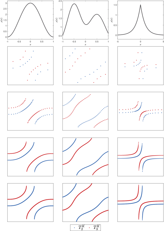
Figure 3: Marginals (the first row) and approximated transport maps (the remaining four rows) in 1D $N=3$ systems; left to right: systems with $\rho_{1},\rho_{2},\rho_{3}$. The maps in the last four rows correspond to rows in Table 2 (a) where $K=12,48,192,768$. The blue and red dots are images of $T_{2}^{K}$ and $T_{3}^{K}$ over grid barycenters, respectively.

The convergence of the GGR approach can be observed as the meshes being refined. Note that explicit solutions of the original MMOT problems are known for 1D systems [42], our results can match the theory perfectly. We also list the output energies and the calculated average errors (the “err_e” column) at each step in Table 2 (a), supporting the efficiency of our approach.

The second set includes three systems, each of which contains 7 particles ($N=7$). Note that this particle number is already intractable if one tries to solve the original MMOT problem Eq. 1 directly. The single-electron densities (marginals) are given by

$$\rho_{4}(x)=c_{4}e^{-x^{2}/\sqrt{\pi}},\quad \Omega=[-2,2],$$

$$\rho_{5}(x)=c_{5}\big{(}e^{-3(x+3)^{2}}+e^{-3(x+2)^{2}}+e^{-2(x+1)^{2}}+e^{-x^{2}}+e^{-2(x-1)^{2}}$$

$$\qquad\qquad+e^{-3(x-2)^{2}}+e^{-3(x-3)^{2}}\big{)}, \Omega=[-4,4],$$

$$\rho_{6}(x)=c_{6}\big{(}e^{-8(x+2.7)^{2}}+e^{-8(x+2.025)^{2}}+e^{-8(x+1.35)^{2}}+e^{-8(x+0.675)^{2}}$$

$$\qquad\qquad+e^{-5(x-0.5)^{2}}+e^{-5(x-1.5)^{2}}+e^{-5(x-2.5)^{2}}\big{)},\quad \Omega=[-3,3],$$

respectively, with $c_{i},~{}i=4,5,6,$ the normalization constants such that $\int_{\Omega}\rho_{i}(x)~{}{\rm d}x=7$. The last two examples can be viewed as systems with localized electrons, where each Gaussian represents the distribution of an electron. The number of grid points used for the initial meshes is $K^{(0)}=14$ for these three systems.

We show the single-electron densities (marginals) and the convergence of the GGR approach during the mesh refinements in Figure 4.

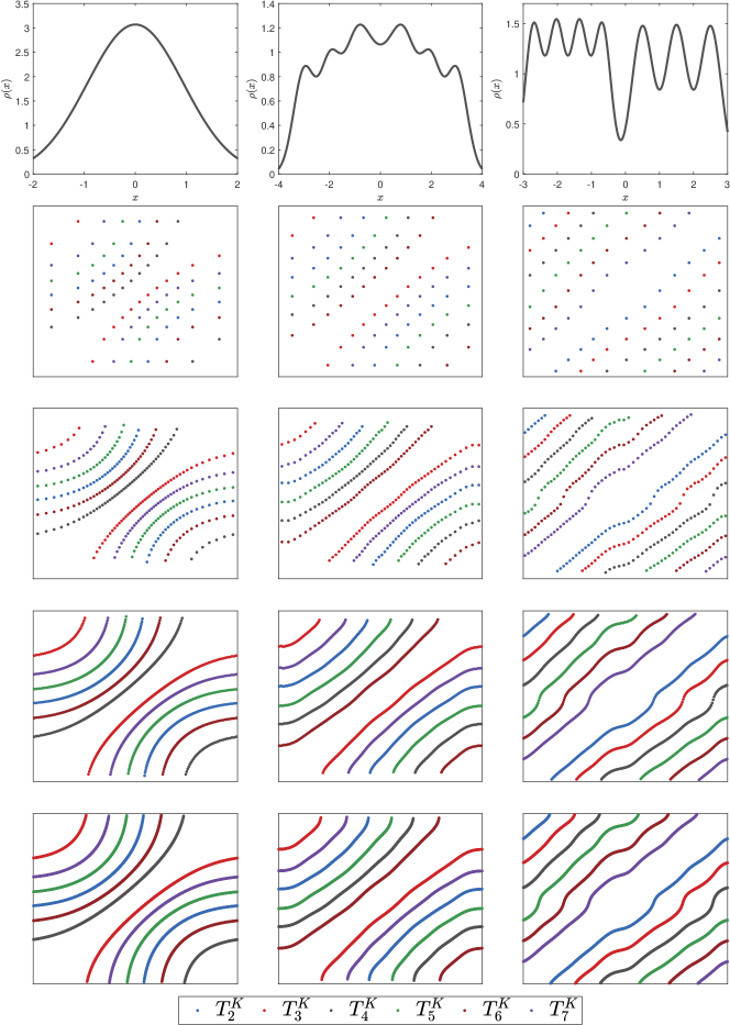
Figure 4: Marginals (the first row) and approximated transport maps (the remaining four rows) in 1D $N=7$ systems; left to right: systems with $\rho_{4},\rho_{5},\rho_{6}$. The maps in the last four rows correspond to rows in Table 2 (b) where $K=14,56,224,896$. The blue, red, black, green, brown and purple dots are images of $T_{i}^{K},~{}i=2,\ldots,7$ over grid barycenters, respectively.

We also list the output energies and the calculated average errors at each step in Table 2 (b). We observe from the numerical results that the iterates given by our GGR approach converge well to the correct solutions.

Table 2: Output energies and calculated average errors of the GGR approach on 1D systems

Step	System 1				System 2				System 3
	$K$	E	err_s	err_e	$K$	E	err_s	err_e	$K$	E	err_s	err_e
GGR_Init	12	18.114	-	0.031	12	12.211	-	0.012	12	6.024	-	0.040
GGR_LS(1)	24	18.911	0.049	0.013	24	12.373	0.041	0.011	24	6.318	0.053	0.018
GGR_LS(2)	48	19.004	0.022	0.009	48	12.367	0.026	0.012	48	6.389	0.027	0.013
GGR_LS(3)	96	19.019	0.014	0.004	96	12.360	0.017	0.009	96	6.400	0.026	0.011
GGR_LS(4)	192	19.021	0.007	0.003	192	12.358	0.010	0.003	192	6.403	0.013	0.001
GGR_LS(5)	384	19.022	0.007	0.002	384	12.358	0.005	0.001	384	6.404	0.003	0.000
GGR_LS(6)	768	19.022	0.004	0.001	768	12.357	0.003	0.001	768	6.404	0.001	0.000

(a) $N=3$

Step	System 4				System 5				System 6
	$K$	E	err_s	err_e	$K$	E	err_s	err_e	$K$	E	err_s	err_e
GGR_Init	14	189.626	-	0.018	14	80.266	-	0.021	14	91.536	-	0.016
GGR_LS(1)	28	193.703	0.027	0.023	28	82.199	0.024	0.012	28	93.056	0.022	0.025
GGR_LS(2)	56	193.312	0.019	0.026	56	81.937	0.012	0.012	56	92.458	0.025	0.019
GGR_LS(3)	112	193.128	0.022	0.016	112	81.854	0.010	0.014	112	92.245	0.019	0.013
GGR_LS(4)	224	193.066	0.015	0.010	224	81.817	0.014	0.011	224	92.185	0.020	0.007
GGR_LS(5)	448	193.044	0.007	0.004	448	81.808	0.009	0.002	448	92.171	0.007	0.003
GGR_LS(6)	896	193.039	0.002	0.002	896	81.806	0.001	0.002	896	92.167	0.003	0.001

(b) $N=7$

To show that the GR subroutine yields high-quality initialization, we compute the average errors of the initial points (the “err_s” column) as well; the notation “-” in the GGR_Init step indicates no initial point is fed to global solver. The decreasing err_s’s underline the efficacy of the GR subroutine, which boosts the GGR approach and helps us find global solutions. Incidentally, the comparison between err_s and err_e in the same row highlights the improvements due to the local solver PBCD. Meanwhile, one can see that err_e is sometimes slightly larger than err_s. In these cases, PBCD eliminates infeasibility while inheriting the high quality of initial points.

4.3 Numerical results on 2D systems

We then consider some 2D systems with the GGR approach. We use the finite elements package FreeFEM [23] to generate the initial meshes for the marginal discretization. The meshes are non-uniform such that every element carries almost the same mass. In the later loops of the GGR approach, each element is refined in the same manner.

The two systems under consideration both consist of 3 particles ($N=3$), whose single-electron densities (marginals) are given by

$$\rho_{7}(x,y)=c_{7}\big{(}e^{-2.5\left|(x,y)-(-1.5,0)\right|^{2}}+0.5e^{-2.5\left|(x,y)-(1.5,0)\right|^{2}}\big{)},\quad \Omega=[-3,3]\times[-2,2],$$

$$\rho_{8}(x,y)=c_{8}\big{(}e^{-2.5\left|(x,y)-(-1.032,-0.84)\right|^{2})}+e^{-2.5\left|(x,y)-(0,0.96)\right|^{2}}$$

$$\qquad\qquad+e^{-2.5\left|(x,y)-(1.032,-0.84)\right|^{2}}\big{)},\quad \Omega=[-2.5,2.5]^{2},$$

respectively, with $c_{i},~{}i=7,8,$ the normalizing factors such that $\int_{\Omega}\rho_{i}(x,y)~{}{\rm d}x~{}{\rm d}y=7$. For the first 2D system, $\rho_{7}$ corresponds to a system that has two electrons located on the left part of $\Omega$ (represented by the first Gaussian centered at $(-1.5,0)$), and the third electron located on the right part (represented by the second Gaussian centered at $(1.5,0)$). For the second 2D system, $\rho_{8}$ corresponds to a system that has three electrons concentrated on three different sites $(-1.032,-0.84)$, $(0,0.96)$ and $(1.032,-0.84)$ (represented by three Gaussians), respectively. The electron densities (marginals) and the corresponding initial meshes (obtained by FreeFEM) are shown in the first two rows of Figure 5. The numbers of grid points used for the initial meshes are $K^{(0)}=240$ for $\rho_{7}$ and $K^{(0)}=170$ for $\rho_{8}$, respectively. After three steps in Framework 1, we reach $K^{(3)}=15360$ for $\rho_{7}$ and $K^{(3)}=10880$ for $\rho_{8}$, respectively.

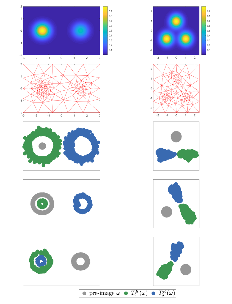
Figure 5: Contours of marginals (the first row), initial meshes (the second row) and slices of approximated transport maps (the third-fifth row) in 2D systems; left to right: systems with $\rho_{7},\rho_{8}$. In system 7-8, we calculated $K$ to 15360 and 10880, respectively. The gray, blue and green circles are pre-images $\omega\subseteq\Omega$, $T_{2}^{K}(\omega)$ and $T_{3}^{K}(\omega)$, respectively.

Table 3: Output energies of the GGR approach on 2D systems

Step	System 7		System 8
	$K$	E	$K$	E
GGR_Init	240	9.503	170	9.491
GGR_LS(1)	960	9.577	680	9.533
GGR_LS(2)	3840	9.598	2720	9.543
GGR_LS(3)	15360	9.604	10880	9.546

To show our results on the 2D systems, in the remaining three rows of Figure 5, we plot the images of the barycenters of triangular elements within some given regions $\omega\subseteq\Omega$, where $T^{K}_{2}$ and $T^{K}_{3}$ are the approximated transport maps Eq. 12 given by the GGR approach. For the two-Gaussian system $\rho_{7}$, the pictures show that: if the first electron is around the left Gaussian center, then the third electron will go to the region near the right Gaussian center, and the second electron will lie in the left part (to satisfy the marginal constraints) but stay away from the first one ($\omega$ and $T^{K}_{2}(\omega)$ lie in two different regions around the left Gaussian center); if one electron is located around the right Gaussian center, then the other two electrons will be around the left Gaussian center while keeping distance away from each other. For the three-Gaussian system $\rho_{8}$, we can see that if one electron is located around one of the Gaussian centers, then the other two electrons go to the other two Gaussian centers, respectively. We also list the output energies at each step in Table 3. Though there are no theoretical results for comparison, our simulations match physical intuitions quite well and can support the reliability of our approach.

5 Conclusions

In the present work, we consider the MMOT problem with Coulomb cost arising in quantum physics. The Monge-like ansatz tides us over curse of dimensionality, in that the number of unknowns scales linearly w.r.t. the number of electrons, however resulting in MPGCC. In quest for global solutions, we propose a global optimization approach GGR for dealing with the derived MPGCC. The GGR approach solves the problem step by step along with the process of mesh refinement, and is equipped with an initialization subroutine such that global solutions are amenable to the proposed local solver PBCD. The convergence property of PBCD is established in the presence of iterate infeasibility. We corroborate the merits of the GGR approach with numerical simulations on several typical 1D and 2D physical systems. Notably, we obtain solutions with high resolution in the 1D cases, and visualize the optimal transport maps in the 2D context.

Appendix A Discretization of (6)

For the repulsive energy in Eq. 6, we have for any $i\in\{2,\ldots,N\}$,

$$\int_{\Omega}\int_{\Omega}\frac{\rho(\boldsymbol{r})\gamma_{i}(\boldsymbol{r},\boldsymbol{r}^{\prime})}{\left|\boldsymbol{r}-\boldsymbol{r}^{\prime}\right|}~{}{\rm d}\boldsymbol{r}~{}{\rm d}\boldsymbol{r}^{\prime}=\sum_{j,k}\int_{e_{k}}\int_{e_{j}}\frac{\rho(\boldsymbol{r})\gamma_{i}(\boldsymbol{r},\boldsymbol{r}^{\prime})}{\left|\boldsymbol{r}-\boldsymbol{r}^{\prime}\right|}~{}{\rm d}\boldsymbol{r}~{}{\rm d}\boldsymbol{r}^{\prime}.$$

Note when $k=j$, the integral explodes and hence we impose $x_{kk}^{i}=0,~{}\forall~{}k$ as extra constraints to avoid numerical instability. In the sequent derivation, we take $\gamma_{i}(\boldsymbol{r},\boldsymbol{r}^{\prime})=0$ whenever $\boldsymbol{r}$ and $\boldsymbol{r}^{\prime}$ belong to the same element:

$$\int_{\Omega}\int_{\Omega}\frac{\rho(\boldsymbol{r})\gamma_{i}(\boldsymbol{r},\boldsymbol{r}^{\prime})}{\left|\boldsymbol{r}-\boldsymbol{r}^{\prime}\right|}~{}{\rm d}\boldsymbol{r}~{}{\rm d}\boldsymbol{r}^{\prime}= \sum_{j\neq k}\int_{e_{k}}\int_{e_{j}}\frac{\rho(\boldsymbol{r})\gamma_{i}(\boldsymbol{r},\boldsymbol{r}^{\prime})}{\left|\boldsymbol{r}-\boldsymbol{r}^{\prime}\right|}~{}{\rm d}\boldsymbol{r}~{}{\rm d}\boldsymbol{r}^{\prime}$$

$$= \sum_{j\neq k}\varrho_{j}x_{i,jk}\int_{e_{k}}\int_{e_{j}}\frac{1}{\left|\boldsymbol{r}-\boldsymbol{r}^{\prime}\right|}~{}{\rm d}\boldsymbol{r}~{}{\rm d}\boldsymbol{r}^{\prime}+O(h)$$

(19) $$= \sum_{j\neq k}\varrho_{j}x_{i,jk}r_{jk}\left|e_{j}\right|\left|e_{k}\right|+O(h)=\left\langle X_{i},\Lambda\Xi C\Xi\right\rangle+O(h),$$

where $h:=\|e\|_{\infty}$ represents the size of the largest element. By similar reasoning, we can write for any $i,j\in\{2,\ldots,N\}:i\neq j$,

$$\int_{\Omega}\int_{\Omega}\int_{\Omega}\frac{\rho(\boldsymbol{r})\gamma_{i}(\boldsymbol{r},\boldsymbol{r}^{\prime})\gamma_{j}(\boldsymbol{r},\boldsymbol{r}^{\prime\prime})}{\left|\boldsymbol{r}^{\prime}-\boldsymbol{r}^{\prime\prime}\right|}~{}{\rm d}\boldsymbol{r}~{}{\rm d}\boldsymbol{r}^{\prime}~{}{\rm d}\boldsymbol{r}^{\prime\prime}$$

(20) $$= \sum_{m,n,t:n\neq t}\varrho_{m}x_{i,mn}x_{j,mt}r_{nt}\left|e_{m}\right|\left|e_{n}\right|\left|e_{t}\right|+O(h)$$

$$= \left\langle X_{i},\Xi\Lambda X_{j}\Xi C\Xi\right\rangle+O(h).$$

Note that we have excluded $n=t$ cases and impose $\left\langle X_{i},X_{j}\right\rangle=0$ as extra complementarity constraints. By Eq. 19 and Eq. 20, the repulsive energy in Eq. 6 can be approximated by

$$\sum_{2\leq i\leq N}\left\langle X_{i},\Lambda\Xi C\Xi\right\rangle+\sum_{i<j}\left\langle X_{i},\Xi\Lambda X_{j}\Xi C\Xi\right\rangle,$$

with error depending on the size of the largest element.

Regarding normalizing and marginal constraints in Eq. 5, we can see from similar derivation that, for any $i\in\{2,\ldots,N\}$,

$$1=\frac{1}{\left|e_{j}\right|}\int_{e_{j}}1~{}{\rm d}\boldsymbol{r} =\frac{1}{\left|e_{j}\right|}\int_{e_{j}}\int_{\Omega}\gamma_{i}(\boldsymbol{r},\boldsymbol{r}^{\prime})~{}{\rm d}\boldsymbol{r}^{\prime}~{}{\rm d}\boldsymbol{r}=\sum_{k=1}^{K}x_{i,jk}\left|e_{k}\right|,~{}\forall j,$$

$$\varrho_{k}=\frac{1}{\left|e_{k}\right|}\int_{e_{k}}\rho(\boldsymbol{r}^{\prime})~{}{\rm d}\boldsymbol{r}^{\prime} =\frac{1}{\left|e_{k}\right|}\int_{e_{k}}\int_{\Omega}\rho(\boldsymbol{r})\gamma_{i}(\boldsymbol{r},\boldsymbol{r}^{\prime})~{}{\rm d}\boldsymbol{r}~{}{\rm d}\boldsymbol{r}^{\prime}=\sum_{j=1}^{K}\varrho_{j}x_{i,jk}\left|e_{j}\right|+O(h),~{}\forall k.$$

Consequently, the constraints in Eq. 5 can be approximated using

$$X_{i}e=\mathbf{1},~{}X_{i}^{\top}\Xi\rho=\rho,~{}\forall~{}i\in\{2,\ldots,N\}.$$

References

- [1] A. Alfonsi, R. Coyaud, and V. Ehrlacher, Constrained overdamped Langevin dynamics for symmetric multimarginal optimal transportation, Feb. 2021, https://arxiv.org/abs/2102.03091.
- [2] A. Alfonsi, R. Coyaud, V. Ehrlacher, and D. Lombardi, Approximation of optimal transport problems with marginal moments constraints, Math. Comp., 90 (2021), pp. 689–737, https://doi.org/10.1090/mcom/3568.
- [3] A. Becke, Perspective: fifty years of density-functional theory in chemical physics, J. Chem. Phys., 140 (2014), 18A301 (18 pages), https://doi.org/10.1063/1.4869598.
- [4] S. Bednarek, B. Szafran, T. Chwiej, and J. Adamowski, Effective interaction for charge carriers confined in quasi-one-dimensional nanostructures, Phys. Rev. B, 68 (2003), 045328 (9 pages), https://doi.org/10.1103/PhysRevB.68.045328.
- [5] J.-D. Benamou, G. Carlier, and L. Nenna, A numerical method to solve multi-marginal optimal transport problems with Coulomb cost, in Splitting Methods in Communication, Imaging, Science, and Engineering, Springer, Cham, 2016, p. 577–601, https://doi.org/10.1007/978-3-319-41589-5_17.
- [6] J. Bolte, S. Sabach, and M. Teboulle, Proximal alternating linearized minimization for nonconvex and nonsmooth problems, Math. Program., 146 (2014), pp. 459–494, https://doi.org/10.1007/s10107-013-0701-9.
- [7] G. Buttazzo, L. Pascale, and P. Gori-Giorgi, Optimal-transport formulation of electronic density-functional theory, Phys. Rev. A, 85 (2012), 062502 (11 pages), https://doi.org/10.1103/PhysRevA.85.062502.
- [8] R. Byrd, J. Nocedal, and R. Waltz, Knitro: an integrated package for nonlinear optimization, in Large-Scale Nonlinear Optimization, Springer, Boston, MA, 2006, pp. 35–59, https://doi.org/10.1007/0-387-30065-1_4.
- [9] H. Chen and G. Friesecke, Pair densities in density functional theory, Multiscale Model. Simul., 13 (2015), pp. 1259–1289, https://doi.org/10.1137/15M1014024.
- [10] H. Chen, G. Friesecke, and C. Mendl, Numerical methods for a Kohn-Sham density functional model based on optimal transport, J. Chem. Theory Comput., 10 (2014), pp. 4360–4368, https://doi.org/10.1021/ct500586q.
- [11] M. Colombo, L. Pascale, and S. Marino, Multimarginal optimal transport maps for one–dimensional repulsive costs, Can. J. Math., 67 (2015), pp. 350–368, https://doi.org/10.4153/CJM-2014-011-x.
- [12] C. Cotar, G. Friesecke, and C. Klüppelberg, Density functional theory and optimal transportation with Coulomb cost, Commun. Pure Appl. Math., 66 (2013), pp. 548–599, https://doi.org/10.1002/cpa.21437.
- [13] C. Cotar, G. Friesecke, and B. Pass, Infinite-body optimal transport with Coulomb cost, Calc. Var., 54 (2015), pp. 717–742, https://doi.org/10.1007/s00526-014-0803-0.
- [14] F. Facchinei, H. Jiang, and L. Qi, A smoothing method for mathematical programs with equilibrium constraints, Math. Program., 85 (1999), pp. 107–134, https://doi.org/10.1007/s10107990015a.
- [15] M. Flegel and C. Kanzow, On the Guignard constraint qualification for mathematical programs with equilibrium constraints, Optimization, 54 (2005), pp. 517–534, https://doi.org/10.1080/02331930500342591.
- [16] R. Fletcher and S. Leyffer, Nonlinear programming without a penalty function, Math. Program., 91 (2002), pp. 239–269, https://doi.org/10.1007/s101070100244.
- [17] R. Fletcher and S. Leyffer, Solving mathematical programs with complementarity constraints as nonlinear programs, Optim. Methods Softw., 19 (2004), pp. 15–40, https://doi.org/10.1080/10556780410001654241.
- [18] R. Fourer, D. Gay, and B. Kernighan, A modeling language for mathematical programming, Manage. Sci., 36 (1990), pp. 519–641, https://doi.org/10.1287/mnsc.36.5.519.
- [19] G. Friesecke, A. Schulz, and D. Vögler, Genetic column generation: fast computation of high-dimensional multi-marginal optimal transport problems, Mar. 2021, https://arxiv.org/abs/2103.12624.
- [20] G. Friesecke and D. Vögler, Breaking the curse of dimension in multi-marginal kantorovich optimal transport on finite state spaces, SIAM J. Math. Anal., 50 (2018), pp. 3996–4019, https://doi.org/10.1137/17M1150025.
- [21] J. Grossi, D. Kooi, K. Giesbertz, M. Seidl, A. Cohen, P. Mori-Sánchez, and P. Gori-Giorgi, Fermionic statistics in the strongly correlated limit of density functional theory, J. Chem. Theory Comput., 13 (2017), pp. 6089–6100, https://doi.org/10.1021/acs.jctc.7b00998.
- [22] E. Gur, S. Sabach, and S. Shtern, Convergent nested alternating minimization algorithms for non-convex optimization problems. https://ssabach.net.technion.ac.il/files/2020/11/GSS2020-1.pdf, 2020.
- [23] F. Hecht, New development in freefem++, J. Numer. Math., 20 (2012), pp. 251–265, https://doi.org/10.1515/jnum-2012-0013, https://freefem.org/.
- [24] F. Hickernell and Y. Yuan, A simple multistart algorithm for global optimization, Operations Research Transactions (China), 1 (1997), pp. 1–12, http://citeseerx.ist.psu.edu/viewdoc/summary?doi=10.1.1.46.1346.
- [25] T. Hoheisel, C. Kanzow, and A. Schwartz, Theoretical and numerical comparison of relaxation methods for mathematical programs with complementarity constraints, Math. Program., 137 (2013), pp. 257–288, https://doi.org/10.1007/s10107-011-0488-5.
- [26] X. Hu and D. Ralph, Convergence of a penalty method for mathematical programming with complementarity constraints, J. Optim. Theory Appl., 123 (2004), pp. 365–390, https://doi.org/10.1007/s10957-004-5154-0.
- [27] X. Jia, C. Kanzow, P. Mehlitz, and G. Wachsmuth, An augmented Lagrangian method for optimization problems with structured geometric constraints, May 2021, https://arxiv.org/abs/2105.08317.
- [28] C. Kanzow and A. Schwartz, The price of inexactness: convergence properties of relaxation methods for mathematical programs with complementarity constraints revisited, Math. Oper. Res., 40 (2015), pp. 253–275, https://doi.org/10.1287/moor.2014.0667.
- [29] Y. Khoo, L. Lin, M. Lindsey, and L. Ying, Semidefinite relaxation of multimarginal optimal transport for strictly correlated electrons in second quantization, SIAM J. Sci. Comput., 42 (2020), pp. B1462–B1489, https://doi.org/10.1137/20M1310977.
- [30] Y. Khoo and L. Ying, Convex relaxation approaches for strictly correlated density functional theory, SIAM J. Sci. Comput., 41 (2019), pp. B773–B795, https://doi.org/10.1137/18M1207478.
- [31] X. Li, D. Sun, and K.-C. Toh, On the efficient computation of a generalized Jacobian of the projector over the Birkhoff polytope, Math. Program., 179 (2020), pp. 419–446, https://doi.org/10.1007/s10107-018-1342-9.
- [32] F. Malet and P. Gori-Giorgi, Strong correlation in Kohn-Sham density functional theory, Phys. Rev. Lett., 109 (2012), 246402 (5 pages), https://doi.org/10.1103/PhysRevLett.109.246402.
- [33] C. Mendl and L. Lin, Kantorovich dual solution for strictly correlated electrons in atoms and molecules, Phys. Rev. B, 87 (2013), 125106 (6 pages), https://doi.org/10.1103/PhysRevB.87.125106.
- [34] C. Mendl, F. Malet, and P. Gori-Giorgi, Wigner localization in quantum dots from Kohn-Sham density functional theory without symmetry breaking, Phys. Rev. B, 89 (2014), 125106 (8 pages), https://doi.org/10.1103/PhysRevB.89.125106.
- [35] G. Monge, Mémoire sur la Théorie des Déblais et des Remblais, Histoire Acad. Sciences, 1781.
- [36] P. Pardalos and S. Vavasis, Quadratic programming with one negative eigenvalue is NP-hard, J. Glob. Optim., 1 (1991), pp. 15–22, https://doi.org/10.1007/BF00120662.
- [37] F. Santambrogio, Optimal Transport for Applied Mathematicians, Birkhäuser, Cham, 2015, https://doi.org/10.1007/978-3-319-20828-2.
- [38] H. Scheel and S. Scholtes, Mathematical programs with complementarity constraints: stationarity, optimality, and sensitivity, Math. Oper. Res., 25 (2000), pp. 1–22, https://doi.org/10.1287/moor.25.1.1.15213.
- [39] S. Scholtes, Convergence properties of a regularization scheme for mathematical programs with complementarity constraints, SIAM J. Optim., 11 (2001), pp. 918–936, https://doi.org/10.1137/S1052623499361233.
- [40] S. Scholtes and M. Stöhr, Exact penalization of mathematical programs with equilibrium constraints, SIAM J. Control Optim., 37 (1999), pp. 617–652, https://doi.org/10.1137/S0363012996306121.
- [41] M. Seidl, Strong-interaction limit of density-functional theory, Phys. Rev. A, 60 (1999), pp. 4387–4395, https://doi.org/10.1103/PhysRevA.60.4387.
- [42] M. Seidl, P. Gori-Giorgi, and A. Savin, Strictly correlated electrons in density-functional theory: a general formulation with applications to spherical densities, Phys. Rev. A, 75 (2007), 042511 (12 pages), https://doi.org/10.1103/PhysRevA.75.042511.
- [43] M. Seidl, S. Marino, A. Gerolin, L. Nenna, K. Giesbertz, and P. Gori-Giorgi, The strictly-correlated electron functional for spherically symmetric systems revisited, Feb. 2017, https://arxiv.org/abs/1702.05022.
- [44] C. Villani, Optimal Transport: Old and New, vol. 338, Springer, Berlin, Heidelberg, 2009, https://doi.org/10.1007/978-3-540-71050-9.
- [45] R. Waltz, J. Morales, J. Nocedal, and D. Orban, An interior algorithm for nonlinear optimization that combines line search and trust region steps, Math. Program., 107 (2006), pp. 391–408, https://doi.org/10.1007/s10107-004-0560-5.
- [46] Y. Xu and W. Yin, A block coordinate descent method for regularized multiconvex optimization with applications to nonnegative tensor factorization and completion, SIAM J. Imaging Sci., 6 (2013), pp. 1758–1789, https://doi.org/10.1137/120887795.
- [47] J. Ye, Necessary and sufficient optimality conditions for mathematical programs with equilibrium constraints, J. Math. Anal. Appl., 307 (2005), pp. 350–369, https://doi.org/10.1016/j.jmaa.2004.10.032.