Fast value iteration for energy games

Abstract

We propose a variant of an algorithm introduced by Schewe and also studied by Luttenberger for solving parity or mean-payoff games. We present it over energy games and call it fast value iteration. We find that using potential reductions as introduced by Gurvich, Karzanov and Khachiyan allows for a simple and elegant presentation of the algorithm, which repeatedly applies a natural generalisation of Dijkstra’s algorithm to the two-player setting due to Khachiyan, Gurvich and Zhao.

1 Introduction

Mean-payoff and energy games.

In the games under study, two players, Min and Max, take turns in moving a token over a sinkless finite directed graph whose edges are labelled by (potentially negative) integers, interpreted as payoffs. In a mean-payoff game, the players aim to optimise (minimising or maximising, respectively) the average payoff in the long run. When playing an energy game, Min and Max optimise the supremum of the cumulative sum of payoffs which takes values in $[0,+\infty]$.

These two games are determined [17]: for each initial vertex $v$, there is a value $x\in\mathbb{R}$ such that starting from $v$, the minimiser can ensure an outcome not greater than $x$ whereas the maximiser can ensure at least $x$. We call these values, respectively, the mean-payoff and the energy value of the vertex $v$. They are moreover uniformly positionaly determined [8, 3] which means that the players can achieve the optimal value from each vertex by using a single strategy depending only on the current position in the game. We refer to Figure 1 for a complete example.

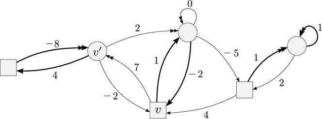
Figure 1: Example of a game; circles and squares represent vertices which respectively belong to Min and Max. Mean-payoff values, from left to right, are $-2,-2,-\frac{1}{2},-\frac{1}{2},1$ and $1$, and mean-payoff-optimal positional strategies for both players are identified in bold. Energy values, from left to right, are $0,2,9,0,\infty$ and $\infty$, and energy-optimal strategies are given by arrows with double heads.

In this paper, we are interested in the problem of computing energy values of the vertices in a given game, which we call solving the energy game. As a consequence of positional determinacy, the energy value of a vertex is finite if and only if its mean-payoff value is non-positive [4], and therefore solving an energy game also solves the so called threshold problem for mean-payoff games (determining if the mean-payoff value is non-positive). In fact, all state of the art algorithms [4, 7, 2] for the threshold problem – further discussed below – actually go through solving the energy game. The best algorithms for the more general problems of computing the exact values or synthesising optimal strategies in the mean-payoff game also rely on solving several instances of auxiliary energy games [6].

Positional strategies achieving positive or non-positive mean-payoff values can be checked in polynomial time, and therefore the threshold problem belongs to $\mathrm{NP}\cap\mathrm{coNP}$. Despite numerous efforts, no polynomial algorithm is known. Mean-payoff games are known [23] to be more general than parity games [9, 20] which enjoy a similar complexity status but were recently shown to be solvable in quasipolynomial time [5]. It is however unlikely that algorithms for solving parity games in quasipolynomial time generalise to mean-payoff games [10].

Schewe’s algorithm.

Schewe presented in [24] a strategy improvement algorithm for solving parity games. Schewe points out that his framework can be adapted to the more general case of mean-payoff games; one can actually see it as a switching policy in the combinatorial strategy improvement framework proposed by Björklund and Vorobiov [2]. Luttenberger [15] later formulated the same algorithm as one iterating over non-deterministic strategies: over such strategies, it can be rephrased as iterative applications of the natural “all-switch” policy.

At that time, the connection between mean-payoff and energy games – established only later in [3] and then simplified in [4] – was not well understood. In particular, the algorithms above, following [2], introduce an additional sink vertex, called retreat vertex, and restrict the iteration to so called admissible strategies, which can be understood as those guaranteeing a finite energy. Actually, Björklund and Vorobiov [2] ask in their conclusion whether one can avoid the need for a retreat vertex and admissible strategies; a positive answer to this question is provided by the energy valuation presented in this work (details are provided in the PhD thesis [22] of Ohlmann).

Our contribution.

We propose a variant of Schewe’s algorithm; while the main ideas are the same, the presentation as well as the precise execution of the algorithm differ. In particular, we do not require introducing a retreat vertex, or restrict to a subclass of strategies. We also do not require the vocabulary from strategy improvement.

The algorithm is presented as one iterating successive potential reductions, as introduced by Gurvich, Karzanov and Khachiyan [13], until obtaining a trivial game. Each iteration solves an auxiliary game over only non-negative weights, which is done in $O(m+n\log n)$ operations using a simple extension of Dijkstra’s algorithm to the two-player setting, due to Khachiyan, Gurvich and Zhao [14].

We believe that our new approach presents three advantages:

• Our version is conceptually simpler and allows to appreciate the core algorithmic idea in a new light. It also lends itself to more straightforward implementations of an algorithm which performs very well in practice.

• Stating the algorithm in terms of potential reductions allows to compare it to other important algorithms for solving energy games, such as those of Brim et al [4] and of Gurvich, Karzanov and Khachiyan [13, 21].

• Our presentation leads to a natural symmetric extension of the algorithm; we refer to the conclusion for more details.

Related work.

It is worth noting that Schewe’s algorithm is a key component in the LTL-synthesis tool STRIX [19, 16], which has won all editions of the main annual synthesis competition SYNTCOMP. The algorithm was also ported to the GPU by Meyer and Luttenberger [18]. We also believe that there are similarities to be understood between the algorithm under study and the quasi-dominion approach of Benerecetti, Dell’Erba and Mogavero [1].

Outline.

The first section introduces all necessary concepts and recalls the relationship between mean-payoff and energy games. We also present the standard value iteration algorithm of Brim et al. [4] in the vocabulary of potential reductions. The second section presents the fast value iteration algorithm, and the third one proves its correctness and termination. We then conclude and discuss future work.

2 Preliminaries

In this preliminary section, we introduce mean-payoff and energy games, as well as potential reductions.

Mean-payoff and energy games.

In this paper, a game is a tuple $\mathcal{G}=(G,w,V_{\mathrm{Min}},V_{\mathrm{Max}})$, where $G=(V,E\subseteq V\times V)$ is a finite directed graph with no sink, $w:E\to\mathbb{Z}$ is a labelling of its edges by integer weights, and $V_{\mathrm{Min}},V_{\mathrm{Max}}$ is a partition of $V$. We always use $n,m$ and $W$ respectively for $|V|,|E|$ and $\max\limits_{e\in E}|w(e)|$; we say that vertices in $V_{\mathrm{Min}}$ belong to Min while those in $V_{\mathrm{Max}}$ belong to Max. We now fix a game $\mathcal{G}=(G,w,V_{\mathrm{Min}},V_{\mathrm{Max}})$.

A path is a (possibly empty, possibly infinite) sequence of edges $\pi=e_{0}e_{1}\dots$ with matching endpoints, that is, there is a sequence of vertices $v_{0}v_{1}\dots$ such that $e_{i}=v_{i}v_{i+1}$. For convenience, we often write $v_{0}\rightarrow v_{1}\rightarrow v_{2}\rightarrow\dots$ for such a path. Given a finite or infinite path $\pi=e_{0}e_{1}\dots$ we let $w(\pi)=w(e_{0})w(e_{1})\dots$ denote the sequence of weights appearing on $\pi$. The sum of a finite path $\pi$ is the sum of the weights appearing on it, we denote it by $\mathrm{sum}(\pi)$.

Given a finite or infinite path $\pi=e_{0}e_{1}\dots=v_{0}\rightarrow v_{1}\rightarrow\dots$ and an integer $k\geq 0$, we let $\pi_{<k}=e_{0}e_{1}\dots e_{k-1}=v_{0}\rightarrow v_{1}\rightarrow\dots\rightarrow v_{k}$, and we let $\pi_{\leq k}=\pi_{<k+1}$. Note that $\pi_{<0}$ is the empty path, and that $\pi_{<k}$ has length $k$ in general: it belongs to $E^{k}$. We say that $\pi$ starts in $v_{0}$, and when it is finite and of length $k$ that it ends in $v_{k}$. By convention, the empty path starts and ends in all vertices. A cycle is a finite path which starts and ends in the same vertex. A finite path $v_{0}\rightarrow v_{1}\rightarrow\dots\rightarrow v_{k}$ is simple if there is no repetition in $v_{0},v_{1},\dots,v_{k-1}$; note that a cycle may be simple. We let $\Pi_{v}^{\omega}$ denote the set of infinite paths starting in $v$.

The greek letter $\omega$ denotes the ordered set of positive integers. We use $\mathbb{R}^{\infty},\mathbb{Z}^{\infty}$ and $\mathbb{N}^{\infty}$ to denote respectively $\mathbb{R}\cup\{\infty\},\mathbb{Z}\cup\{\infty\}$ and $\mathbb{N}\cup\{\infty\}$. A valuation is a map $\mathrm{val}:\mathbb{Z}^{\omega}\to\mathbb{R}^{\infty}$ which assigns a potentially infinite real number to each infinite sequence of weights.

The three valuations which are studied in this paper are the mean-payoff, energy, and positive-energy valuations, given by

$$\begin{array}[]{lclcl}\mathrm{MP}(w_{0}w_{1}\dots)&=&\limsup_{k}\frac{1}{k}\sum_{i=0}^{k-1}w_{i}&\in&\mathbb{R},\\ \mathrm{En}(w_{0}w_{1}\dots)&=&\sup_{k}\sum_{i=0}^{k-1}w_{i}&\in&\mathbb{N}^{\infty},\\ \mathrm{En}^{+}(w_{0}w_{1}\dots)&=&\sum_{i=0}^{k_{\text{neg}}-1}w_{i}&\in&\mathbb{N}^{\infty},\end{array}$$

where $k_{\text{neg}}=\min\{k\mid w_{k}<0\}\in\mathbb{N}^{\infty}$ is the first index corresponding to a negative weight. For technical convenience, and only in the context of energy games, we will also consider games in which weights are potentially (positively) infinite. We thus extend the definitions of $\mathrm{En}$ and $\mathrm{En}^{+}$ to words in $(\mathbb{Z}^{\infty})^{\omega}$, using the same formula. Note that for any $w\in(\mathbb{Z}^{\infty})^{\omega}$ we have $0\leq\mathrm{En}^{+}\leq\mathrm{En}$. The three valuations are illustrated on a given weight profile in Figure 2.

Figure 2: The three valuations over a given weight-profile. The mean-payoff value is given by the slope of the green line, which corresponds to the long-term average. In this case, the mean-payoff is $\leq 0$, and both $\mathrm{En}$ and $\mathrm{En}^{+}$ are finite.

A strategy for Min is a map $\sigma:V_{\mathrm{Min}}\to E$ such that for all $v\in V_{\mathrm{Min}}$, it holds that $\sigma(v)$ is an edge outgoing from $v$. We say that a (finite or infinite) path $\pi=e_{0}e_{1}\dots=v_{0}\rightarrow v_{1}\rightarrow\dots$ is consistent with $\sigma$ if whenever $v_{i}\in V_{\mathrm{Min}}$, it holds that $e_{i}=\sigma(v_{i})$. We write in this case $\pi\models\sigma$. Strategies for Max are defined similarly and written $\tau:V_{\mathrm{Max}}\to E$. Paths consistent with Max strategies are defined analogously and also denoted by $\pi\models\tau$. In common vocabulary, the theorem below states that the three valuations are determined with positional strategies over finite games. It is well known for $\mathrm{MP}$ and $\mathrm{En}$ and easy to prove for $\mathrm{En}^{+}$ (Lemma 3.1 provides an algorithmic proof of this fact). We remark that positional determinacy also holds for the two energy valuations $\mathrm{En}$ and $\mathrm{En}^{+}$ over games where we allow for infinite weights.

Theorem 2.1 ([8, 3]).

For each $\mathrm{val}\in\{\mathrm{MP},\mathrm{En},\mathrm{En}^{+}\}$, there exist strategies $\sigma_{0}$ for Min and $\tau_{0}$ for Max such that for all $v\in V$ we have

$$\sup_{\pi\models\sigma_{0}}\mathrm{val}(w(\pi))=\inf_{\sigma}\sup_{\pi\models\sigma}\mathrm{val}(w(\pi))=\sup_{\tau}\inf_{\pi\models\tau}\mathrm{val}(w(\pi))=\inf_{\pi\models\tau_{0}}\mathrm{val}(w(\pi)),$$

where $\sigma,\tau$ and $\pi$ respectively range over strategies for Min, strategies for Max, and infinite paths from $v$.

The quantity defined by the equilibrium above is called the value of $v$ in the $\mathrm{val}$ game, and we denote it by $\mathrm{val}_{\mathcal{G}}(v)\in\mathbb{R}^{\infty}$; strategies $\sigma_{0}$ and $\tau_{0}$ verifying the equalities above are called $\mathrm{val}$-optimal, note that they do not depend on $v$.

The following result relates the values in the mean-payoff and energy games; this direct consequence of Theorem 2.1 was first stated in [4].

Corollary 2.2 ([4]).

For all $v\in V$ it holds that

$$\mathrm{MP}_{\mathcal{G}}(v)\leq 0\iff\mathrm{En}_{\mathcal{G}}(v)<\infty\iff\mathrm{En}_{\mathcal{G}}(v)\leq(n-1)W.$$

Therefore computing $\mathrm{En}$ values of the games is harder than the threshold problem. As explained in the introduction, all state-of-the-art algorithms for the threshold problem actually compute $\mathrm{En}$ values. This shifts our focus from mean-payoff to energy games.

Potential reductions.

We fix a game $\mathcal{G}=(G=(V,E),w,V_{\mathrm{Min}},V_{\mathrm{Max}})$. A potential is a map $\phi:V\to\mathbb{N}^{\infty}$. Potentials are partially ordered coordinatewise. Given an edge $vv^{\prime}\in E$, we define its $\phi$-modified weight to be

$$w_{\phi}(vv^{\prime})=\begin{cases}\infty&\text{ if }\phi(v),\phi^{\prime}(v)\text{ or }w(vv^{\prime})\text{ is }\infty\\ w(vv^{\prime})+\phi(v^{\prime})-\phi(v)&\text{ otherwise}.\end{cases}$$

The $\phi$-modified game $\mathcal{G}_{\phi}$ is simply the game $(G,w_{\phi},V_{\mathrm{Min}},V_{\mathrm{Max}})$; informally, all weights are replaced by the modified weights. Note that the underlying graph does not change, in particular paths in $\mathcal{G}$ and $\mathcal{G}_{\phi}$ are the same. Note that any edge outgoing a vertex $v$ with potential $\phi(v)=\infty$ has weight $\infty$ in the modified game, therefore $v$ has $\mathrm{En}$ and $\mathrm{En}^{+}$-values $\infty$ in $G_{\phi}$.

Observe that for a finite path $\pi=v_{0}\rightarrow v_{1}\rightarrow\dots\rightarrow v_{k}$ which visits only vertices with finite potential, its sum in $\mathcal{G}_{\phi}$ is given by

$$\mathrm{sum}_{\phi}(v)=\mathrm{sum}(\pi)+\phi(v_{k})-\phi(v_{0}).$$

We let $0$ denote the constant zero potential; note that $\mathcal{G}_{0}=\mathcal{G}$. For convenience, we use $\mathrm{En}_{\phi}$ to denote $\mathrm{En}_{\mathcal{G}_{\phi}}$ (we remark that $\mathrm{En}_{0}=\mathrm{En}_{\mathcal{G}}$). We will omit the subscript whenever the game or potential under consideration is clear from the context.

Moving from $\mathcal{G}$ to $\mathcal{G}_{\phi}$ for a given potential $\phi$ is called a potential reduction; these were introduced by Gallai [12] for studying network related problems such as shortest-paths problems. In the context of mean-payoff or energy games, they were introduced in [13] and later rediscovered numerous times. The main result that allows to use potential reductions to solve energy games is stated as follows.

Theorem 2.3.

If $\phi$ satisfies $\phi\leq\mathrm{En}_{0}$, then it holds that $\mathrm{En}_{0}=\phi+\mathrm{En}_{\phi}$ over $V$.

We will use the following lemma to prove Theorem 2.3.

Lemma 2.4.

Let $\sigma_{0}$ be an $\mathrm{En}$-optimal Min strategy in $\mathcal{G}$ and $\pi=v_{0}\rightarrow v_{1}\rightarrow\dots\rightarrow v_{k}$ be a finite path consistent with $\sigma_{0}$ such that $\mathrm{En}_{0}(v_{k})<\infty$. Then we have $\mathrm{sum}(\pi)\leq\mathrm{En}_{0}(v_{0})-\mathrm{En}_{0}(v_{k})$.

Proof 2.5.

Let $\pi^{\prime}$ be an infinite path from $v_{k}$ consistent with $\sigma_{0}$ and such that $\mathrm{En}_{0}(v_{k})=\mathrm{En}(w(\pi^{\prime}))$ (such a path exists, as it can be obtained from an $\mathrm{En}$-optimal Max strategy $\tau_{0}$). Then $\pi\pi^{\prime}$ is consistent with $\sigma_{0}$ thus $\mathrm{En}_{0}(v_{0})\geq\mathrm{En}(w(\pi\pi^{\prime}))$ by optimality. We thus obtain

$$\begin{array}[]{lcl}\mathrm{En}_{0}(v_{0})\ \ \geq\ \ \mathrm{En}(w(\pi\pi^{\prime}))&=&\sup_{k^{\prime}\geq 0}(\mathrm{sum}((\pi\pi^{\prime})_{<k^{\prime}}))\\ &\geq&\sup_{k^{\prime}\geq k}(\mathrm{sum}((\pi\pi^{\prime})_{<k^{\prime}}))\\ &=&\mathrm{sum}(\pi)+\sup_{k^{\prime}\geq 0}\mathrm{sum}(\pi^{\prime}_{<k^{\prime}})\\ &=&\mathrm{sum}(\pi)+\mathrm{En}(w(\pi^{\prime}))\ \ =\ \ \mathrm{sum}(\pi)+\mathrm{En}_{0}(v_{k}).\end{array}$$

We now present a proof of Theorem 2.3.

Proof 2.6 (Proof of Theorem 2.3).

Let $\phi:V\to\mathbb{N}^{\infty}$ be a potential such that $\phi\leq\mathrm{En}_{0}$; we aim to prove that $\mathrm{En}_{0}=\phi+\mathrm{En}_{\phi}$ over $V$. Consider first a vertex $v$ with $\mathrm{En}_{0}(v)=\infty$, fix an optimal Max strategy $\tau_{0}$ in $\mathcal{G}$ and an infinite path $\pi=e_{0}e_{1}\dots=v_{0}\rightarrow v_{1}\rightarrow\dots$ consistent with $\tau_{0}$ from $v$: by definition we have $\mathrm{En}(w(\pi))=\sup_{k}\sum_{i=0}^{k-1}w(e_{i})=\infty$. We claim that $\mathrm{En}(w_{\phi}(\pi))=\infty$ which proves the wanted equality over $v$ (both terms are infinite).

• If for some $i$, $w(e_{i})=\infty$ then $w_{\phi}(e_{i})=\infty$ which implies the result.

• If for some $i$, $\phi(v_{i})=\infty$ then again we have $w_{\phi}(e_{i})=\infty$.

• Otherwise, we have for all $k$

  $$\mathrm{sum}_{\phi}(\pi_{<k})=\underbrace{\phi(v_{k})-\phi(v_{0})}_{\text{bounded}}+\mathrm{sum}(\pi_{<k}),$$

  and therefore $\sup_{k}\mathrm{sum}_{\phi}(\pi_{<k})=\sup_{k}\mathrm{sum}(\pi_{<k})=\infty$, the wanted result.

We now consider a vertex $v$ such that $\mathrm{En}_{0}(v)<\infty$. Consider an $\mathrm{En}$-optimal Min strategy $\sigma_{0}:V_{\mathrm{Min}}\to E$ in $\mathcal{G}$ and let $\pi=v_{0}\rightarrow v_{1}\rightarrow\dots$ be an infinite path consistent with $\sigma_{0}$ starting from $v_{0}=v$. Note that for any $k\geq 0$, $v_{k}$ has finite energy value, and thus we obtain thanks to Lemma 2.4 and the hypothesis $\phi\leq\mathrm{En}_{0}$ that

$$\begin{array}[]{lcl}\mathrm{sum}_{\phi}(\pi_{<k})&=&\mathrm{sum}(\pi_{<k})+\phi(v_{k})-\phi(v_{0})\\ &\leq&\mathrm{En}_{0}(v_{0})\underbrace{-\mathrm{En}_{0}(v_{k})+\phi(v_{k})}_{\leq 0}-\phi(v_{0})\ \ \leq\ \ \mathrm{En}_{0}(v_{0})-\phi(v_{0}),\end{array}$$

hence $\mathrm{En}_{\phi}(v_{0})=\sup_{\pi\models\sigma_{0}}\sup_{k\geq 0}\mathrm{sum}_{\phi}(\pi_{<k})\leq\mathrm{En}_{0}(v_{0})-\phi(v_{0})$.

For the other inequality, consider an optimal Min strategy $\sigma_{\phi}$ in $\mathcal{G}_{\phi}$, and let $\pi$ be an infinite path from $v_{0}=v$ consistent with $\sigma_{\phi}$. By applying Lemma 2.4 in $\mathcal{G}_{\phi}$ we now get

$$\begin{array}[]{lcl}\mathrm{sum}(\pi_{<k})&=&\mathrm{sum}_{\phi}(\pi_{<k})-\phi(v_{k})+\phi(v_{0})\\ &\leq&\mathrm{En}_{\phi}(v_{0})-\underbrace{\mathrm{En}_{\phi}(v_{k})}_{\geq 0}-\underbrace{\phi(v_{k})}_{\geq 0}+\phi(v_{0})\ \ \leq\ \ \mathrm{En}_{\phi}(v_{0})+\phi(v_{0}),\end{array}$$

and the wanted result follows by taking a supremum.

An illustration of the effect of potential reductions over energy values, described in Theorem 2.3, is given in Figure 3.

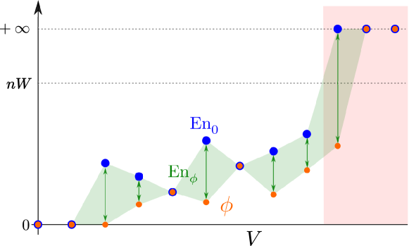
Figure 3: An illustration of the effect of potential reductions in the energy values. The energy value $\mathrm{En}_{\phi}(v)$ of $v$ in the $\phi$-modified game $\mathcal{G}_{\phi}$ is given by the difference between $\mathrm{En}_{0}(v)$ and $\phi(v)$. For the three vertices on the right, energy values in both games are $\infty$.

We say that a potential $\phi$ is sound if it satisfies the hypothesis of Theorem 2.3: $\phi\leq\mathrm{En}_{0}$.

Observe that $(\mathcal{G}_{\phi})_{\phi^{\prime}}=\mathcal{G}_{\phi+\phi^{\prime}}$: sequential applications of potential reductions correspond to reducing with respect to the sum of the potentials. Moreover, if $\phi$ is sound for $\mathcal{G}$ and $\phi^{\prime}$ is sound for $\mathcal{G}_{\phi}$, then applying Theorem 2.3 twice yields $\mathrm{En}_{0}=\phi+\phi^{\prime}+\mathrm{En}_{\phi+\phi^{\prime}}$.

The value iteration of Brim et al.

Before moving on to the fast value iteration, it is instructive to describe the standard one of Brim et al. [4] as follows. Consider the valuation $\mathrm{First}$ given by

$$\mathrm{First}(w_{0}w_{1}\dots)=\max(w_{0},0)\in\mathbb{N}.$$

Note that $\mathrm{First}$ depends only on the first weight appearing on the path, therefore the $\mathrm{First}$-values of the vertices of a game $\mathcal{G}$ can be computed in linear time $O(m)$: the $\mathrm{First}$-value of a Min vertex (resp. a Max vertex) $v$ is the minimum (resp. the maximum) of $\max(w(vv^{\prime}),0)$ over its successors $v^{\prime}$.

Now for any infinite sequence of weights $w=w_{0}w_{1}\dots$ we have $\mathrm{First}(w)\leq\mathrm{En}(w)$, and therefore the $\mathrm{First}$-values of a game $\mathcal{G}$ do not exceed its $\mathrm{En}$-values. Stated differently, $\mathrm{First}:V\to\mathbb{N}^{\infty}$ defines a sound potential . The value iteration algorithm of Brim et al. simply iterates the corresponding potential transformation, generating a sequence of modified games. The iteration terminates when for all vertices of the obtained game, if their cumulative sum of potentials computed so far is $\leq nN$, then their $\mathrm{First}$-value is $0$ (the $\mathrm{En}$-value in the original game of those vertices is the cumulative sum of potentials; the rest of them have $\mathrm{En}$-value $\infty$).

Simple games.

A game is simple if all simple cycles have nonzero sum. The following result is folklore and states that one may reduce to a simple game at the cost of a linear blow up in $W$. It holds thanks to the fact that positive mean-payoff values are $\geq 1/n$, which is a well-known consequence of Theorem 2.1.

Lemma 2.7.

Let $\mathcal{G}=(G,w,V_{\mathrm{Min}},V_{\mathrm{Max}})$ be an arbitrary game. The game with modified weights $\mathcal{G}^{\prime}=(G,(n+1)w-1,V_{\mathrm{Min}},V_{\mathrm{Max}})$ is simple and has the same vertices of positive mean-payoff values as $\mathcal{G}$.

Note moreover that simplicity is preserved by potential transformations, since sums of weights over cycles are left unchanged.

3 The fast value iteration algorithm

3.1 Presentation of the algorithm

The fast value iteration algorithm is based on successively applying sound potential reductions $\phi_{0},\dots,\phi_{j}$ until a game $\mathcal{G}^{\prime}$ is reached where energy-values are either 0 or $\infty$. Thanks to Theorem 2.3, we have $\mathrm{En}_{\mathcal{G}}=\mathrm{En}_{\mathcal{G}^{\prime}}+\phi_{0}+\dots+\phi_{j}$; in particular, a vertex has finite energy (or non-positive mean-payoff) in $\mathcal{G}$ if and only if it has energy 0 in $\mathcal{G}^{\prime}$, and in this case its energy in $\mathcal{G}$ is given by $\phi_{0}(v)+\dots+\phi_{j}(v)$.

The potential reductions computed by each iteration of the fast value iteration algorithm are precisely the $\mathrm{En}^{+}$-values in the game. Intuitively, the players optimise the (non-negative) sum of the weights seen before the first negative weight. Since $0\leq\mathrm{En}^{+}\leq\mathrm{En}$, the potential $\mathrm{En}^{+}:V\to\mathbb{N}^{\infty}$ is indeed sound, as required by our approach. Note that we have $\mathrm{First}\leq\mathrm{En}^{+}$: the algorithm performs bigger steps than the standard value iteration of Brim et al. [4] (hence the name). The algorithm terminates when the next potential reductions does not produce any change in the game. Lemma 3.5 shows that this condition implies that the energy-values of the obtained game are either $0$ or $\infty$.

The fact that the $\mathrm{En}^{+}$-values can be computed efficiently follows from the fact that only non-negative weights are considered, and therefore a straightforward two-player extension of Dijkstra’s algorithm, due to Khachiyan, Gurvich and Zhao [14] can be applied. A similar subroutine was also given by Schewe [24], whereas Luttenberger [15] uses an adaptation of the algorithm of Bellman-Ford which is less efficient.

Lemma 3.1 (Based on [14]).

Over simple games, the $\mathrm{En}^{+}$-values can be computed in $O(m+n\log n)$ operations.

Proof 3.2.

We start by determining in linear time $O(m)$ the set $N$ of vertices from which Min can force to immediately visit an edge of negative weight; these have $\mathrm{En}^{+}$-value 0. We will successively update a set $F$ containing the set of vertices over which $\mathrm{En}^{+}$ is currently known. We initialise this set $F$ to $N$. Note that all remaining Min vertices have only non-negative outgoing edges, and all remaining Max vertices have (at least) a non-negative outgoing edge.

We then iterate the two following steps illustrated in Figure 4. (A complexity analysis is given below.)

1. If there is a Max vertex $v\notin F$ all of whose non-negative outgoing edges $vv^{\prime}$ lead to $F$, set $\mathrm{En}^{+}(v)$ to be the maximal $w(vv^{\prime})+\mathrm{En}^{+}(v^{\prime})$, add $v$ to $F$, and go back to 1.

2. Otherwise, let $vv^{\prime}$ be an edge from $V_{\mathrm{Min}}\setminus F$ to $F$ (it is necessarily positive) minimising $w(vv^{\prime})+\mathrm{En}^{+}(v^{\prime})$; set $\mathrm{En}^{+}(v)=w(vv^{\prime})+\mathrm{En}^{+}(v^{\prime})$, add $v$ to $F$ and go back to 1. If there is no such edge, terminate.

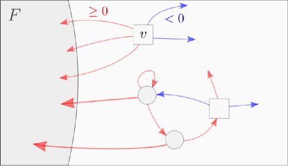
Figure 4: The game version of Dijkstra’s algorithm; blue edges are negative and red ones are non-negative. If there is a vertex such as $v$ (it belongs to $\mathrm{Max}$ and all edges pointing out of $F$ are $<0$), one may set the value of $v$. Otherwise, set the value of a Min vertex $v$ minimising $w(vv^{\prime})+\mathrm{En}^{+}(v^{\prime})$ over edges going to $F$; if there is no such edge, terminate (Max can force seeing $\geq 0$ edges forever).

After the iteration has terminated, there remains to deal with ${F}^{\mathsf{c}}$, which is the set of vertices from which Max can ensure to visit only non-negative edges forever. Since the arena is assumed to be simple (no simple cycle has weight zero) it holds that $\mathrm{En}^{+}$ is $\infty$ over ${F}^{\mathsf{c}}$, and we are done.

As is standard, by storing the number of edges outgoing from Max vertices in ${F}^{\mathsf{c}}$ to $F$, step 1 induces only a total linear runtime $O(m)$. For step 2, one should store, for each $v\in V_{\mathrm{Max}}\setminus F$, the edge towards $F$ minimising $w(vv^{\prime})+\mathrm{En}^{+}(v^{\prime})$ in a priority queue. Using a Fibonacci heap as was first suggested by Fredman and Tarjan [11] for Dijkstra’s algorithm lowers the complexity from $O(m\log n)$ to $O(m+n\log n)$.

3.2 Termination and correctness

Termination.

To prove that the fast value iteration algorithm terminates in finitely many steps, we rely on a simple lemma which states that the set of vertices from which Min can ensure to immediately see a negative weight can only shrink throughout the iteration. This will allow us to show that the cumulative sum of the $\mathrm{En}^{+}$-values is bounded, proving the termination of the algorithm.

Lemma 3.3.

Let $\mathcal{G}^{\prime}=\mathcal{G}_{\mathrm{En}_{\mathcal{G}}^{+}}$, let $N$ and $N^{\prime}$ be the sets of vertices from which Min can ensure to immediately visit a negative weight, respectively in $\mathcal{G}$ and $\mathcal{G}^{\prime}$. We have $N^{\prime}\subseteq N$.

Proof 3.4.

We show that ${N}^{\mathsf{c}}\subseteq{N^{\prime}}^{\mathsf{c}}$. Let $v\in{N}^{\mathsf{c}}$. If $\mathrm{En}^{+}_{\mathcal{G}}(v)=\infty$, then $v$ has only outgoing edges of infinite weight in $\mathcal{G}^{\prime}$ thus is cannot belong to $N^{\prime}$; we assume otherwise.

• Assume $v\in V_{\mathrm{Max}}$. Let $\tau$ be an $\mathrm{En}^{+}_{\mathcal{G}}$-optimal strategy in $\mathcal{G}$, and let $\tau(v)=vv^{\prime}\in E$. Since $v\notin N$ we have $w(vv^{\prime})\geq 0$ and $\mathrm{En}^{+}_{\mathcal{G}}(v)=w(vv^{\prime})+\mathrm{En}^{+}_{\mathcal{G}}(v^{\prime})$. Hence we have $w_{\mathrm{En}^{+}_{\mathcal{G}}}(vv^{\prime})=w(vv^{\prime})+\mathrm{En}^{+}_{\mathcal{G}}(v^{\prime})-\mathrm{En}^{+}_{\mathcal{G}}(v)=0\geq 0$ so $v\notin N^{\prime}$.

• Assume now that $v\in V_{\mathrm{Min}}$. We have for all $vv^{\prime}\in E$ that $w(vv^{\prime})\geq 0$ hence $\mathrm{En}^{+}_{\mathcal{G}}(v)\leq w(vv^{\prime})+\mathrm{En}^{+}_{\mathcal{G}}(v^{\prime})$, and thus $w_{\mathrm{En}^{+}_{\mathcal{G}}}(vv^{\prime})\geq 0$, so $v\notin N^{\prime}$.

We now let $\mathcal{G}_{0}=\mathcal{G}$ denote the initial game, and for each $j\geq 0$ we let $\phi_{j}=\mathrm{En}_{\mathcal{G}_{j}}^{+}$ and $\mathcal{G}_{j+1}=(\mathcal{G}_{j})_{\phi_{j}}$ be the game obtained after $j$ iterations of the algorithm. We also let $\Phi_{j}=\phi_{0}+\dots+\phi_{j-1}$; it holds that $\mathcal{G}_{j}=(\mathcal{G}_{0})_{\Phi_{j}}$.

This lemma directly gives (with obvious notations) $N_{0}\supseteq N_{1}\supseteq\dots$ and therefore vertices $v^{\prime}$ in $N_{j}$ satisfy $\Phi_{j}(v^{\prime})=0$. Now if $v$ is a vertex such that $\phi_{j}(v)=\mathrm{En}_{\mathcal{G}_{j}}^{+}(v)$ is finite, then by definition there is a simple path $\pi=v_{0}\rightarrow\dots\rightarrow v_{k}$ in $\mathcal{G}$ from $v$ to some $v^{\prime}\in N_{j}$ whose $\Phi_{j}$-modified sum is $\mathrm{sum}_{\Phi_{j}}(\pi)=\phi_{j}(v)$. This rewrites as

$$0\leq\phi_{j}(v)=-\Phi_{j}(v)+\underbrace{\Phi_{j}(v^{\prime})}_{0}+\underbrace{\sum_{i=0}^{k-1}w_{\Phi_{j}}(v_{i}v_{i+1})}_{\leq nW},$$

and thus $\Phi_{j}(v)\leq nW$. Stated differently, finite values remain $\leq nW$, which guarantees termination in at most $O(n^{2}N)$ iterations.

We give a full example over a game of size 15 in Figure 5.

Figure 5: A complete execution of the fast value iteration algorithm. In each iteration, we indicate the $\mathrm{En}^{+}$-values of each vertex. Optimal strategies are indicated with bold arrows. Vertices from which Min can force to immediately see a negative weight are coloured in blue, and those with a strictly positive $\mathrm{En}^{+}$-value in red.

Correctness.

Recall that the iteration terminates after $j$ steps if $\Phi_{j+1}=\Phi_{j}$ (where $\Phi_{j}=\phi_{0}+\dots+\phi_{j-1}$ is the cumulative sum of the $\mathrm{En}^{+}$-values at the $j$-th iteration). We now state and prove correctness of the termination condition.

Lemma 3.5.

If $\Phi_{j+1}=\Phi_{j}$, then $\mathrm{En}_{\mathcal{G}_{j}}$ takes values in $\{0,\infty\}$ over $V$.

Proof 3.6.

Note that vertices such that $\Phi_{j}(v)=\infty$ have only outgoing edges of weight $\infty$ in $\mathcal{G}_{j}$ and therefore they have $\mathrm{En}^{+}$-value $\infty$. Hence, $\Phi_{j}(v)<\infty\Rightarrow\mathrm{En}^{+}_{\mathcal{G}_{j}}(v)=0$; we let $F$ be the set of vertices $v$ with $\Phi_{j}(v)<\infty$. Since $\Phi_{j+1}=\Phi_{j}$, all Min vertices in $F$ have a non-positive outgoing edge in $\mathcal{G}_{j}$ towards $F$, and all Max vertices in $F$ have all their outgoing edges non-positive and towards $F$, hence the result.

4 Conclusion

We have presented the fast value iteration algorithm using potential reductions. This allows to reduce to several iterations over non-negative weights, each of which can be treated efficiently using Dijkstra’s algorithm. In particular, presenting the algorithm does not require introducing a retreat vertex, or using vocabulary from strategy improvements. We believe that this new presentation sheds a lot of clarity on this important algorithmic idea.

Alternating value iteration.

We end the paper with a possible extension of these ideas. One may also compute, in the very same fashion, the $\mathrm{En}^{-}$-values of the game, where $\mathrm{En}^{-}:\mathbb{Z}^{\omega}\to[-\infty,0]$ is given by $\mathrm{En}^{-}(w_{0}w_{1}\dots)=\sum_{i=0}^{k_{\text{pos}}-1}w_{i}$, with $k_{\text{pos}}=\min\{k\mid w_{k}>0\}$. Iterating $\mathrm{En}^{-}$ potential transformations gives rise to a dual algorithm, which of course terminates with similar complexity.

We have observed empirically that alternatively applying $\mathrm{En}^{+}$ and $\mathrm{En}^{-}$ potential transformation leads an algorithm which terminates over any instance. Moreover, it achieves even fewer iterations that the (asymmetric) fast value iteration algorithm, and especially so over parity games, for which we have witnessed a significant gain over large random instances.

However, we have not been able to derive its termination using the currently available tools. Could one prove termination of the (symmetric) alternating value iteration algorithm? Could we hope for a subexponential combinatorial upper bound?

References

- [1] Massimo Benerecetti, Daniele Dell’Erba, and Fabio Mogavero. Solving mean-payoff games via quasi dominions. In TACAS, volume 12079 of Lecture Notes in Computer Science, pages 289–306. Springer, 2020.
- [2] Henrik Björklund and Sergei G. Vorobyov. Combinatorial structure and randomized subexponential algorithms for infinite games. Theor. Comput. Sci., 349(3):347–360, 2005.
- [3] Patricia Bouyer, Ulrich Fahrenberg, Kim Guldstrand Larsen, Nicolas Markey, and Jirí Srba. Infinite runs in weighted timed automata with energy constraints. In FORMATS, volume 5215 of Lecture Notes in Computer Science, pages 33–47. Springer, 2008.
- [4] Lubos Brim, Jakub Chaloupka, Laurent Doyen, Raffaella Gentilini, and Jean-François Raskin. Faster algorithms for mean-payoff games. Formal Methods in System Design, 38(2):97–118, 2011.
- [5] Cristian S. Calude, Sanjay Jain, Bakhadyr Khoussainov, Wei Li, and Frank Stephan. Deciding parity games in quasipolynomial time. In STOC, pages 252–263, 2017.
- [6] Carlo Comin and Romeo Rizzi. Improved pseudo-polynomial bound for the value problem and optimal strategy synthesis in mean payoff games. Algorithmica, 77(4):995–1021, 2017.
- [7] Dani Dorfman, Haim Kaplan, and Uri Zwick. A faster deterministic exponential time algorithm for energy games and mean payoff games. In ICALP, pages 114:1–114:14, 2019.
- [8] A. Ehrenfeucht and J. Mycielski. Positional strategies for mean payoff games. International Journal of Game Theory, 109(8):109–113, 1979.
- [9] E. Allen Emerson and Charanjit S. Jutla. Tree automata, -calculus and determinacy. In FOCS, pages 368–377. IEEE Computer Society, 1991.
- [10] Nathanaël Fijalkow, Paweł Gawrychowski, and Pierre Ohlmann. Value iteration using universal graphs and the complexity of mean payoff games. In MFCS, volume 170 of LIPIcs, pages 34:1–34:15. Schloss Dagstuhl - Leibniz-Zentrum für Informatik, 2020.
- [11] Michael L. Fredman and Robert Endre Tarjan. Fibonacci heaps and their uses in improved network optimization algorithms. In FOCS, pages 338–346. IEEE Computer Society, 1984.
- [12] T. Gallai. Maximum-minimum sätze über graphen. Acta Math. Acad. Sci. Hung., (9):395–434, 1958.
- [13] V. A. Gurvich, A. V. Karzanov, and L. G. Khachiyan. Cyclic games and an algorithm to find minimax cycle means in directed graphs. USSR Computational Mathematics and Mathematical Physics, 28:85–91, 1988.
- [14] Leonid Khachiyan, Vladimir Gurvich, and Jihui Zhao. Extending Dijkstra’s algorithm to maximize the shortest path by node-wise limited arc interdiction. In CSR, volume 3967 of Lecture Notes in Computer Science, pages 221–234. Springer, 2006.
- [15] M. Luttenberger. Strategy iteration using non-deterministic strategies for solving parity games. CoRR, 2008. URL: http://arxiv.org/abs/0806.2923.
- [16] Michael Luttenberger, Philipp J. Meyer, and Salomon Sickert. Practical synthesis of reactive systems from LTL specifications via parity games. Acta Informatica, 57(1-2):3–36, 2020.
- [17] Donald A. Martin. Borel determinacy. Annals of Mathematics, 102(2):363–371, 1975.
- [18] Philipp J. Meyer and Michael Luttenberger. Solving mean-payoff games on the GPU. In ATVA, volume 9938 of Lecture Notes in Computer Science, pages 262–267, 2016.
- [19] Philipp J. Meyer, Salomon Sickert, and Michael Luttenberger. Strix: Explicit reactive synthesis strikes back! In CAV, volume 10981 of Lecture Notes in Computer Science, pages 578–586. Springer, 2018.
- [20] Andrzej W. Mostowski. Games with forbidden positions. Technical Report 78, University of Gdansk, 1991.
- [21] Pierre Ohlmann. The GKK algorithm is the fastest over simple mean-payoff games. CoRR, abs/2110.04533, 2021. URL: https://arxiv.org/abs/2110.04533, arXiv:2110.04533.
- [22] Pierre Ohlmann. Monotonic graphs for parity and mean-payoff games. PhD thesis, Université de Paris, 2021.
- [23] Anuj Puri. Theory of Hybrid Systems and Discrete Event Systems. PhD thesis, EECS Department, University of California, Berkeley, dec 1995.
- [24] Sven Schewe. An optimal strategy improvement algorithm for solving parity and payoff games. In CSL, volume 5213 of Lecture Notes in Computer Science, pages 369–384. Springer, 2008.