Superconductor in static gravitational, electric and magnetic fields with vortex lattice

Abstract

We estimate the conjectured interaction between the Earth’s gravitational field and a superconductor immersed in external, static electric and magnetic field. The latter is close to the sample upper critical field and generates the presence of a vortex lattice. The proposed interaction could lead to multiple, measurable effects. First of all, a local affection of the gravitational field inside the superconductor could take place. Second, a new component of a generalized electric field parallel to the superconductor surface is generated inside the sample.

The analysis is performed by using the time-dependent Ginzburg–Landau theory combined with the gravito-Maxwell formalism. This approach leads us to analytic solutions of the problem, also providing the average values of the generated fields and corrections inside the sample. We will also study which are the physical parameters to optimize and, in turn, the most suitable materials to maximize the effect.

1  Introduction

The possible interaction between superconductors and gravitational field is an intriguing field of research, providing an interesting connection between condensed matter systems and gravitational interaction, with beneficial effects both in theoretical and applied physics. The seminal paper [1] set the stage for a deeper analysis of the phenomenon, while, in the following years, a certain amount of scientific literature on the subject was produced [2, 3, 4, 5, 6, 7, 8, 9, 10, 11]. The underlying idea behind this line of research is that, under certain conditions, a gravity/supercondensate interplay should exist, resulting in a slight affection of the local gravitational field through the interaction with suitable condensate systems. Finally, in 1992 Podkletnov and Nieminen proposed a laboratory experimental configuration to detect the conjectured mutual interplay [12, 13]. Due the complexity of the experimental setting and the high costs involved, the experiment was then repeated only in simplified versions [14], without achieving conclusive results.

After the above experiments, a series of theoretical explanations have been proposed in the literature [15, 16, 17, 18], including the first and most convincing interpretation [19, 20] given in terms of a coupling of the gravitational field with an unconventional state of matter (superfluid) in a quantum gravity framework. In all these works, the contribution of the superfluid is included in the energy momentum tensor, exploiting the formalism of general relativity. Unfortunately, this approach does not allow to extrapolate quantitative predictions to be put in relation with possible laboratory experiments: one is then led to consider alternative, phenomenological evidences to better understand the proposed interplay.

Parallel to DeWitt (and subsequent) studies about the coupling between supercondensates and gravity, other theoretical [21, 22, 23, 24, 25] and experimental [26, 27, 28] researches were conducted about generalized electric-type fields induced in (super)conductors by the presence of the Earth’s weak gravitational field. The main result of those studies was the introduction of a generalized electric-type field, characterized by an electrical component and a gravitational one, leading to detectable corrections to the free fall of charged particles. These results then led to the definition of a set of generalized, fundamental fields featuring both gravitational and electromagnetic components [29, 30, 31, 32, 33, 34]. This gravito-Maxwell formalism, valid in the weak gravity regime, is particularly suitable for treating the behaviour of a superfluid immersed in the Earth’s gravitational field [35, 36, 37, 38].

In this paper we again use the time-dependent Ginzburg Landau theory combined with the gravito-Maxwell formulation. With respect to our previous analyses, this time we also consider the presence of external static electric and magnetic fields. In particular, the magnetic field value is very close to the critical magnetic field of the superconductor, and its presence also determines the presence of a vortex lattice. These new ingredients can lead to an enhancement of the interaction with the gravitational field, once chosen appropriate sample parameters and geometry.

2  Gravito-Maxwell formalism

Here we consider a weak gravitational background, where the (nearly-flat) spacetime metric $g_{\mu\nu}$ is expressed as

$$g_{\mu\nu}\>\simeq\>\eta_{\mu\nu}+h_{\mu\nu}\>,$$ (2)

with $\eta_{\mu\nu}=\mathrm{diag}(-1,+1,+1,+1)$ and where $h_{\mu\nu}$ is a small perturbation of the flat Minkowski spacetime. If we now introduce the symmetric traceless tensor

$$\bar{h}_{\mu\nu}\>=\>h_{\mu\nu}-\frac{1}{2}\,\eta_{\mu\nu}\,h\>,$$ (3)

with $h=h^{\sigma}{}_{\sigma}$, it can be shown that the Einstein equations in the harmonic De Donder gauge $\partial^{\mu}\bar{h}_{\mu\nu}\simeq 0$ can be rewritten, in linear approximation, as [33, 35, 36, 37, 38]

$$R_{\mu\nu}-\frac{1}{2}\,g_{\mu\nu}\,R\>=\>\partial^{\rho}\mathscr{G}_{\mu\nu\rho}\>=\>8\pi\mathrm{G}\,T_{\mu\nu}\>,$$ (4)

having also defined the tensor

$$\mathscr{G}_{\mu\nu\rho}\>\equiv\>\partial_{{[}\nu}\bar{h}_{\rho{]}\mu}+\partial^{\sigma}\eta_{\mu{[}\rho}\,\bar{h}_{\nu{]}\sigma}\>\simeq\>\partial_{{[}\nu}\bar{h}_{\rho{]}\mu}\>.$$ (5)

2.1  Gravito-Maxwell formulation

We then introduce the fields [29, 33]

$$\mathbf{E}_{\textrm{g}}=-\frac{1}{2}\,\mathscr{G}_{00i}=-\frac{1}{2}\,\partial_{{[}0}\bar{h}_{i{]}0}\,,\qquad\mathbf{A}_{\textrm{g}}=\frac{1}{4}\,\bar{h}_{0i}\,,\qquad\mathbf{B}_{\textrm{g}}=\frac{1}{4}\,{\varepsilon_{i}}^{jk}\,\mathscr{G}_{0jk}\,,$$ (6)

for which we get, restoring physical units, the set of equations [29, 33, 35, 31, 32, 39, 34, 40, 36, 41, 42, 37, 38]

$$\nabla\cdot\mathbf{E}_{\text{g}}=4\pi\mathrm{G}\,\rho_{\text{g}}\,,\qquad\; \nabla\cdot\mathbf{B}_{\text{g}}=0\,,$$ (7)

$$\nabla\times\mathbf{E}_{\text{g}}=-\dfrac{\partial\mathbf{B}_{\text{g}}}{\partial t}\,,\qquad\; \nabla\times\mathbf{B}_{\text{g}}=4\pi\mathrm{G}\,\frac{1}{c^{2}}\,\mathbf{j}_{\text{g}}+\frac{1}{c^{2}}\,\frac{\partial\mathbf{E}_{\text{g}}}{\partial t}\,,$$

having defined the mass density  $\rho_{\text{g}}\equiv-T_{00}$  and the mass current density  $\mathbf{j}_{\text{g}}\equiv T_{0i}$ . The above equations have the same formal structure of the Maxwell equations, with $\mathbf{E}_{\textrm{g}}$ and $\mathbf{B}_{\textrm{g}}$ gravitoelectric and gravitomagnetic field, respectively.

2.2  Generalized fields and equations

Now we introduce generalized electric/magnetic fields, scalar and vector potentials, featuring both electromagnetic and gravitational contributions [29, 30, 33, 35]:

$$\mathbf{E}=\mathbf{E}_{\text{e}}+\frac{m}{e}\,\mathbf{E}_{\text{g}}\,,\qquad\mathbf{B}=\mathbf{B}_{\text{e}}+\frac{m}{e}\,\mathbf{B}_{\text{g}}\,,\qquad\phi=\phi_{\text{e}}+\frac{m}{e}\,\phi_{\text{g}}\,,\qquad\mathbf{A}=\mathbf{A}_{\text{e}}+\frac{m}{e}\,\mathbf{A}_{\text{g}}\,,$$ (8)

where $m$ and $e$ identify the mass and electronic charge, respectively. The generalized Maxwell equations for the new fields read [29, 33, 35, 34, 36, 37, 38]:

$$\nabla\cdot\mathbf{E}=\left(\frac{1}{\varepsilon_{0}}+\frac{1}{\varepsilon_{\text{g}}}\right)\rho\,,\qquad\; \nabla\cdot\mathbf{B}=0\,,$$ (9)

$$\nabla\times\mathbf{E}=-\dfrac{\partial\mathbf{B}}{\partial t}\,,\qquad\; \nabla\times\mathbf{B}=(\mu_{0}+\mu_{\text{g}})\,\mathbf{j}+\frac{1}{c^{2}}\,\frac{\partial\mathbf{E}}{\partial t}\,,$$

where $\varepsilon_{0}$ and $\mu_{0}$ are the vacuum electric permittivity and magnetic permeability. In the above equations, $\rho$ and $\mathbf{j}$ identify the electric charge density and electric current density, respectively, while the mass density and the mass current density vector can be expressed in terms of the latter as

$$\rho_{\text{g}}=\frac{m}{e}\,\rho\,,\qquad\quad\mathbf{j}_{\text{g}}=\frac{m}{e}\>\mathbf{j}\>,$$ (10)

while the vacuum gravitational permittivity $\varepsilon_{\text{g}}$ and permeability $\mu_{\text{g}}$ read

$$\varepsilon_{\text{g}}=\frac{1}{4\pi\mathrm{G}}\,\frac{e^{2}}{m^{2}}\>,\qquad\quad\mu_{\text{g}}=\frac{4\pi\mathrm{G}}{c^{2}}\,\frac{m^{2}}{e^{2}}\>.$$ (11)

3  The model

3.1  Time-dependent Ginzburg–Landau formulation

The time-dependent Ginzburg–Landau equations (TDGL) can be written as [43, 44, 45, 46, 47, 48, 49, 50]:

$$\frac{\hbar^{2}}{2\,m_{\star}}\left(i\,\nabla+\frac{2\,e}{\hbar}\,\mathbf{A}\right)^{\!2}\psi~{}-~{}a\,\psi~{}+~{}b\,\left\lvert\psi\right\rvert^{2}\psi\;=\,-\frac{\hbar^{2}}{2\,m_{\star}\,\mathcal{D}}\left(\frac{\partial}{\partial t}+\frac{2\,i\,e}{\hbar}\,\phi\right)\,\psi\;,$$ (.i)

$$\nabla\times\nabla\times\mathbf{A}~{}-~{}\nabla\times\mathbf{B}_{0}\>=\>\mu_{0}\,\big{(}\mathbf{j}_{\text{n}}+\mathbf{j}_{\text{s}}\big{)}\,,$$ (.ii)

where $\mathbf{B}_{0}$ is the external magnetic field, $\mathcal{D}$ is the diffusion coefficient, $\sigma$ the conductivity in the normal phase and

$$a\>=\>a(T)\>=\>a_{0}\,(T-T_{\textrm{c}})\,,\qquad\qquad b\>=\>b(T_{\textrm{c}})\,,\qquad$$ (13)

$a_{0}$, $b$ being positive constants. The contributions related to the normal current and supercurrent densities can be explicitly written as

$$\begin{split}\mathbf{j}_{\text{n}}&\>=\>-\sigma\left(\frac{\partial\mathbf{A}}{\partial t}+\nabla\phi\right)\>,\\[9.0pt] \mathbf{j}_{\text{s}}&\>=\>-i\,\hbar\,\frac{e}{m_{\star}}\left(\psi^{*}\,\nabla\psi-\psi\,\nabla\psi^{*}\right)-\frac{4\,e^{2}}{m_{\star}}\,\left\lvert\psi\right\rvert^{2}\mathbf{A}\>.\end{split}$$ (14)

Let us put ourselves in the London gauge $\nabla\cdot\mathbf{A}=0$ so that

$$\nabla^{2}\mathbf{A}\>=\>-\mu_{0}\left(\mathbf{j}_{\text{n}}+\mathbf{j}_{\text{s}}\right)\>.$$ (15)

We now consider a sample of thickness $L$ along the (vertical) $\vec{u}_{x}$ direction and very large dimensions along $\vec{u}_{y}$, $\vec{u}_{z}$, see Fig. 1. The sample features a square lattice of vortices, whose axes are directed along the direction of the static magnetic field $\mathbf{B}_{0}$ that we choose to be

$$\mathbf{B}_{0}=B_{0}\,\vec{u}_{z}\>,$$ (16)

together with a vector potential $\mathbf{A}$ of the form

$$\mathbf{A}=B_{0}\,x\,\vec{u}_{y}\>.$$ (17)

We then consider the presence of a constant external (standard) electric field $\mathbf{E}_{0}^{{}^{\text{(e)}}}$ along the $\vec{u}_{x}$ direction, so that a generalized static field $\mathbf{E}_{0}$ can be expressed as

$$\mathbf{E}_{0}\>=\>\mathbf{E}_{0}^{{}^{\text{(e)}}}+\mathbf{E}_{0}^{{}^{\text{(g)}}}\>=\>\left(E_{0}^{{}^{\text{(e)}}}-E_{0}^{{}^{\text{(g)}}}\right)\,\vec{u}_{x}\>=\>\left(E_{0}^{{}^{\text{(e)}}}-\frac{m}{e}\,g\right)\,\vec{u}_{x}\>=\>E_{0}\,\vec{u}_{x}\>,\quad$$ (18)

with a related scalar potential $\phi_{0}\>=\>-E_{0}\,x$.

The boundary and initial conditions are

$$\left.\begin{aligned} \left(i\,\nabla\psi+\frac{2\,e}{\hbar}\,\mathbf{A}\,\psi\right)\cdot\mathbf{n}=0&\cr\hfill\nabla\times\mathbf{A}\cdot\mathbf{n}=\mathbf{B}_{0}\cdot\mathbf{n}&\\[4.5pt] \hfill\mathbf{A}\cdot\mathbf{n}=0&\end{aligned}\;\;\right\}\;\text{on }\partial\Omega\times(0,t)\;,\qquad\quad\left.\begin{aligned} \psi(x,0)&\>=\>\psi_{0}(x)\cr\mathbf{A}(x,0)&\>=\>\mathbf{A}_{0}(x)\end{aligned}\!\!\!\!\right\}\;\text{on }\Omega\;,\qquad$$ (19)

where $\partial\Omega$ is the boundary of a smooth and simply connected domain in $\mathbb{R}^{\textrm{N}}$. We denote by $\mathbf{A}_{0}$ the external vector potential, coinciding with the internal value for $t\leq 0$, i.e. when the sample is in the normal state and the material is very weakly diamagnetic. For $t<0$ we also have $T<T_{\textrm{c}}$ and $B>B_{\textsc{c}{}_{2}}$, while at $t=0$ we still have $T<T_{\textrm{c}}$ but $B\simeq B_{\textsc{c}{}_{2}}$.

If we put ourselves very close to $B_{\textsc{c}{}_{2}}$, it is possible to find a solution of the linearized TDGL equations [51, 52] for the order parameter of the form

$$\psi(x,y,t)\>=\>\sum_{n=-\infty}^{\infty}\!c_{n}\,\exp\left(i\,q\,n\left(y+\frac{E_{0}}{B_{0}}\>t\right)\!\right)\;\>\exp\left(-\frac{1}{2\,\xi(T)}\left(x-\frac{\hbar\,q\,n}{2\,e\,B_{0}}\right)^{\!2}+i\,\frac{e\,E_{0}\,\xi^{2}(T)}{\hbar\,\mathcal{D}}\left(x-\frac{\hbar\,q\,n}{2\,e\,B_{0}}\right)\right)\>.$$ (20)

Since we are very close to $B_{\textsc{c}{}_{2}}$, this solution of the linearized TDGL equations describes the behaviour of an ordered vortex lattice, moving under the influence of the external electric field. For a square lattice, $q$ expresses the distance between adjacent vortices [54]

$$q\>\simeq\>\frac{2\pi}{\xi(T)}\>,$$ (21)

and we can also replace the general $c_{n}$ coefficient with the correspondent $c_{{}_{\Box}}$ expression for the square lattice:

$$c_{n}\;\;\rightarrow\;\;\>c_{{}_{\Box}}=\frac{2\sqrt{2\pi}}{\xi^{2}(T)}\>,$$ (22)

the $c_{{}_{\Box}}$ coefficients being then independent of $n$.

Dimensionless TDGL.

In order to write eqs. (12) in a dimensionless form, the following expressions are introduced:

$$\begin{split}&\psi_{0}^{2}(T)=\frac{\left\lvert a(T)\right\rvert}{b}\,,\qquad\;\xi(T)=\frac{\hbar}{\sqrt{2\,m_{\star}\,|a(T)|}}\,,\qquad\;\lambda(T)=\sqrt{\frac{b\,m_{\star}}{4\mu_{0}|a(T)|\,e^{2}}}\,,\qquad\;\kappa=\frac{\lambda(T)}{\xi(T)}\,,\quad\\[6.0pt] &\tau(T)=\frac{\lambda^{2}(T)}{\mathcal{D}}\,,\qquad\;\eta=\mu_{0}\,\sigma\,\mathcal{D}\,,\qquad\;\;B_{\textsc{c}}(T)=\sqrt{\frac{\mu_{0}\,\left\lvert a(T)\right\rvert^{2}}{b}}=\frac{\hbar}{2\sqrt{2}\,e\,\lambda(T)\,\xi(T)}\,,\end{split}$$ (23)

where $\lambda(T)$, $\xi(T)$ and $B_{\textsc{c}}(T)$ are the penetration depth, coherence length and thermodynamic critical field, respectively. We also define the dimensionless quantities

$$t^{\prime}=\>\frac{t}{\tau}\,,\quad\quad\quad x^{\prime}=\>\frac{x}{\lambda}\,,\quad\quad\quad y^{\prime}=\>\frac{y}{\lambda}\,,\quad\quad\quad x_{0}^{\prime}=\>\frac{x_{0}}{\lambda}\,,\quad\quad\quad\psi^{\prime}=\>\frac{\psi}{\psi_{0}}\,,$$ (24)

and the dimensionless potentials, fields and currents can be expressed as:

$$\mathbf{A}^{\prime}=\frac{\mathbf{A}\,\kappa}{\sqrt{2}\,B_{\textsc{c}}\,\lambda}\,,\qquad\phi^{\prime}=\frac{\phi\,\kappa}{\sqrt{2}\,B_{\textsc{c}}\,\mathcal{D}}\,,\qquad\mathbf{E}^{\prime}=\frac{\mathbf{E}\,\lambda\,\kappa}{\sqrt{2}\,B_{\textsc{c}}\,\mathcal{D}}\,,\qquad\mathbf{B}^{\prime}=\frac{\mathbf{B}\,\kappa}{\sqrt{2}\,B_{\textsc{c}}}\,,\qquad\mathbf{j}^{\prime}=\frac{\mathbf{j}\,\mu_{0}\,\lambda\,\kappa}{\sqrt{2}\,B_{\textsc{c}}}\,.$$ (25)

We now consider the dimensionless version of the London gauge,  $\nabla^{\prime}\cdot\mathbf{A}^{\prime}=0$.  Inserting eqs. 24 and 25 in eqs. (12), provides the dimensionless TDGL equations (we drop the primes for the sake of notational simplicity) in a bounded, smooth and simply connected domain in $\mathbb{R}^{\textrm{N}}$ [43, 44]:

$$\frac{\partial\psi}{\partial t}\,+\,i\,\phi\,\psi\,+\,\kappa^{2}\left(\left\lvert\psi\right\rvert^{2}-1\right)\,\psi\,+\,\left(i\,\nabla+\mathbf{A}\right)^{2}\psi\>=\>0\;,$$ (.i)

$$\nabla\times\nabla\times\mathbf{A}\,-\,\nabla\times\mathbf{B}_{0}\>=\>\mathbf{j}_{\text{n}}+\mathbf{j}_{\text{s}}\>=\,-\,\eta\,\left(\frac{\partial\mathbf{A}}{\partial t}+\nabla\phi\right)-\frac{i}{2}\left(\psi^{*}\nabla\psi-\psi\nabla\psi^{*}\right)-\left\lvert\psi\right\rvert^{2}\mathbf{A}\,,$$ (.ii)

and the boundary and initial conditions (19) become, in the dimensionless form

$$\left.\begin{aligned} \left(i\,\nabla\psi+\mathbf{A}\,\psi\right)\cdot\mathbf{n}=0&\cr\nabla\times\mathbf{A}\cdot\mathbf{n}=\mathbf{B}_{0}\cdot\mathbf{n}&\cr\mathbf{A}\cdot\mathbf{n}=0&\end{aligned}\!\!\!\right\}\;\text{on }\partial\Omega\times(0,t)\;;\qquad\quad\left.\begin{aligned} \psi(x,0)&\>=\>\psi_{0}(x)\cr\mathbf{A}(x,0)&\>=\>\mathbf{A}_{0}(x)\end{aligned}\!\!\!\!\right\}\;\text{on }\Omega\;.\qquad$$ (27)

3.2  Solving dimensionless TDGL

We now discuss how to get an analytic approximate solution to the above dimensionless TDGL.

First of all, we write the following first-order expression for the dimensionless order parameter:

$$\psi(x,y,t)\>=\>\sum_{n=-\infty}^{\infty}\!\left\lvert c_{n}\right\rvert\,\exp\left(i\,q\,n\left(y+\frac{E_{0}}{B_{0}}\>t\right)\!\right)\;\>\exp\left(-\frac{\kappa^{2}}{2}\left(x-n\,x_{0}\right)^{2}+i\,\frac{E_{0}}{\kappa}\left(x-n\,x_{0}\right)\right)\>,$$ (28)

with

$$\left\lvert\psi\right\rvert^{2}\>=\>\sum_{n=-\infty}^{\infty}\!\left\lvert c_{n}\right\rvert^{2}\,\exp\left(-\kappa^{2}\left(x-n\,x_{0}\right)^{2}\right)\>.$$ (29)

The equations for the vector potential components can be written as

$$\begin{split}\frac{\partial^{2}A_{x}(x,t)}{\partial x^{2}}&\>=\>\eta\,\left(\frac{\partial A_{x}(x,t)}{\partial t}-E_{0}\right)+\left(A_{x}(x,t)-\frac{E_{0}}{\kappa}\right)\sum_{n=-\infty}^{\infty}\!\left\lvert c_{n}\right\rvert^{2}\,\exp\Big{(}-\kappa^{2}(x-n\,x_{0})^{2}\Big{)}\>,\\[4.30554pt] \frac{\partial^{2}A_{y}(x,t)}{\partial x^{2}}&\>=\>\eta\,\frac{\partial A_{y}(x,t)}{\partial t}+\sum_{n=-\infty}^{\infty}\!\big{(}A_{y}(x,t)-2\,\pi\,\kappa\,n\,\big{)}\,\left\lvert c_{n}\right\rvert^{2}\,\exp\Big{(}-\kappa^{2}(x-n\,x_{0})^{2}\Big{)}\>,\\[4.30554pt] \frac{\partial^{2}A_{z}(x,t)}{\partial x^{2}}&\>=\>\eta\,\frac{\partial A_{z}(x,t)}{\partial t}+\sum_{n=-\infty}^{\infty}\!\left\lvert c_{n}\right\rvert^{2}\,\exp\Big{(}-\kappa^{2}(x-n\,x_{0})^{2}\Big{)}\>.\end{split}$$ (30)

We now want to obtain explicit solutions for the dimensionless order parameter at first order in $E_{0}$. To this end, we have to estimate the summations

$$\sum_{n=-\infty}^{\infty}\!\left\lvert c_{n}\right\rvert^{2}\,\exp\left(-\kappa^{2}\left(x-n\,x_{0}\right)^{2}\right)\,,\quad\quad\quad\sum_{n=-\infty}^{\infty}\!n\,\left\lvert c_{n}\right\rvert^{2}\,\exp\left(-\kappa^{2}\left(x-n\,x_{0}\right)^{2}\right)\,.$$ (31)

Since we are considering a square vortex lattice, we can replace the general coefficients $c_{n}$ with $c_{{}_{\Box}}$ that, for the case under consideration, can be expressed as [54]

$$c_{{}_{\Box}}^{2}\>=\>2\,\sqrt{2\pi}\,\kappa^{2}\>,$$ (32)

being then a function of $\kappa$ only. Moreover, we are interested in high-$T_{\textrm{c}}$ superconductors, so that we also have large values for the $\kappa$ parameter, $\kappa^{2}\,{\gtrsim}\,10^{4}$. This gives us the following estimates for the above (31):

$$\begin{split}&\sum_{n=-\infty}^{\infty}\!\left\lvert c_{n}\right\rvert^{2}\,\exp\left(-\kappa^{2}\left(x-n\,x_{0}\right)^{2}\right)\>=\>c_{{}_{\Box}}^{2}\,e^{-\kappa^{2}x^{2}}\sum_{n=-\infty}^{\infty}\!e^{-\kappa^{2}n^{2}x_{0}^{2}}\;e^{2\,x\,x_{0}\,n\,\kappa^{2}}\>\simeq\>c_{{}_{\Box}}^{2}\,e^{-\kappa^{2}x^{2}}\>,\\[4.30554pt] &\sum_{n=-\infty}^{\infty}\!n\,\left\lvert c_{n}\right\rvert^{2}\,\exp\left(-\kappa^{2}\left(x-n\,x_{0}\right)^{2}\right)\>\simeq\>0\>,\end{split}$$ (33)

where only the $n=0$ term gives a non negligible contribution in the first summation. Equations (30) can be rewritten

$$\begin{split}\frac{\partial^{2}A_{x}(x,t)}{\partial x^{2}}&\>=\>\eta\,\left(\frac{\partial A_{x}(x,t)}{\partial t}-E_{0}\right)+\left(A_{x}(x,t)-\frac{E_{0}}{\kappa}\right)\,c_{{}_{\Box}}^{2}\,e^{-\kappa^{2}x^{2}}\>,\\[4.30554pt] \frac{\partial^{2}A_{y}(x,t)}{\partial x^{2}}&\>=\>\eta\,\frac{\partial A_{y}(x,t)}{\partial t}+A_{y}(x,t)\,c_{{}_{\Box}}^{2}\,e^{-\kappa^{2}x^{2}}\>,\\[4.30554pt] \frac{\partial^{2}A_{z}(x,t)}{\partial x^{2}}&\>=\>\eta\,\frac{\partial A_{z}(x,t)}{\partial t}+c_{{}_{\Box}}^{2}\,e^{-\kappa^{2}x^{2}}\>.\end{split}$$ (34)

Since we are dealing with materials featuring a very large value for the $\kappa$ parameter, $\kappa^{2}\,{\gtrsim}\,10^{4}$, we can also use the approximation

$$e^{-\kappa^{2}x^{2}}\>\simeq\>\frac{\sqrt{\pi}}{\kappa}\,\delta(x)\>,$$ (35)

and our equation for the vector potential components become

$$\frac{\partial A_{x}(x,t)}{\partial t}\> \simeq\>\frac{1}{\eta}\,\frac{\partial^{2}A_{x}(x,t)}{\partial x^{2}}-\left(A_{x}(x,t)-\frac{E_{0}}{\kappa}\right)\,c_{{}_{\Box}}^{2}\,\frac{\sqrt{\pi}}{\eta\,\kappa}\,\delta(x)+E_{0}\>,$$ (.i)

$$\frac{\partial A_{y}(x,t)}{\partial t}\> \simeq\>\frac{1}{\eta}\,\frac{\partial^{2}A_{y}(x,t)}{\partial x^{2}}-A_{y}(x,t)\>c_{{}_{\Box}}^{2}\,\frac{\sqrt{\pi}}{\eta\,\kappa}\,\delta(x)\>,$$ (.ii)

$$\frac{\partial A_{z}(x,t)}{\partial t}\> \simeq\>\frac{1}{\eta}\,\frac{\partial^{2}A_{z}(x,t)}{\partial x^{2}}-c_{{}_{\Box}}^{2}\,\frac{\sqrt{\pi}}{\eta\,\kappa}\,\delta(x)\>.$$ (.iii)

The initial conditions for the vector potential components are:

$$A_{x}\left(x,\,0\right)=0\,,\qquad\;A_{y}\left(x,\,0\right)=B_{0}\,x\,,\qquad\;A_{z}\left(x,\,0\right)=0\,,$$ (37)

and the generalized electric field $\mathbf{E}$ inside the superconductor can be obtained from

$$\mathbf{E}\>=\>-\frac{\partial\mathbf{A}}{\partial t}-\nabla\phi\>.$$ (38)

Averaging over space.

Let us now study the average effects of the generalized electric field inside the superconductor. To this end, we integrate the vector potential components (36) over the $x$-variable [55].

First, we integrate over $x$ eq. (.iii), for an interval $x\in[-L/2,\,L/2]$ . This gives

$$\frac{\partial\bar{A}_{z}(t)}{\partial t}\>=\>-c_{{}_{\Box}}^{2}\,\frac{\sqrt{\pi}}{\eta\,\kappa\,L}\>,$$ (39)

having defined the averaged component  $\bar{A}_{z}(t)=\frac{1}{L}\!\bigintssss\limits_{{}^{-L/2}}^{{}_{L/2}}\!\!dx\,A_{z}(x,t)$  and having used symmetric conditions for the first derivatives with respect to $x$. The above equation is easily solved as

$$\bar{A}_{z}(t)\>=\>-c_{{}_{\Box}}^{2}\,\frac{\sqrt{\pi}}{\eta\,\kappa\,L}\,t+\bar{A}_{z}(0)\>=\>-c_{{}_{\Box}}^{2}\,\frac{\sqrt{\pi}}{\eta\,\kappa\,L}\,t\>,$$ (40)

having used initial conditions (37) to set $\bar{A}_{z}(0)=0$. This in turn gives for the averaged, generalized electric field $\bar{E}_{z}$ component

$$\bar{E}_{z}\>=\>c_{{}_{\Box}}^{2}\,\frac{\sqrt{\pi}}{\eta\,\kappa\,L}\>=\>\frac{2\sqrt{2}\,\pi\,\kappa}{\eta\,L}\>.$$ (41)

The averaged differential equation for the $\bar{A}_{y}(t)$ component is obtained from (.ii) and reads

$$\frac{\partial\bar{A}_{y}(t)}{\partial t}\>=\>-\bar{A}_{y}(t)\>c_{{}_{\Box}}^{2}\,\frac{\sqrt{\pi}}{\eta\,\kappa\,L}\>,$$ (42)

having used the approximation $A_{y}(0,t)\simeq\bar{A}_{y}(t)$. The above equation would give for the averaged component

$$\bar{A}_{y}(t)\>=\>\bar{A}_{y}(0)\>\exp\left(-c_{{}_{\Box}}^{2}\,\frac{\sqrt{\pi}}{\eta\,\kappa\,L}\>t\right)\>=\>0\>,$$ (43)

using again initial condition (37), the resulting field $\bar{E}_{y}(t)$ being then zero.

Finally, for the vertical component we have from (.i)

$$\frac{\partial\bar{A}_{x}(t)}{\partial t}\>=\>-\left(\frac{\bar{A}_{x}(t)}{L}-\frac{E_{0}}{\kappa}\right)\,c_{{}_{\Box}}^{2}\,\frac{\sqrt{\pi}}{\eta\,\kappa}+E_{0}\>,$$ (44)

that is solved, always using the approximation $A_{x}(0,t)\simeq\bar{A}_{x}(t)$, for

$$\begin{split}\bar{A}_{x}(t)&\>=\>\bar{A}_{x}(0)\,\exp\left(-c_{{}_{\Box}}^{2}\,\frac{\sqrt{\pi}}{\eta\,\kappa\,L}\,t\right)+E_{0}\left(\frac{L}{\kappa}+\frac{\eta\,\kappa\,L}{c_{{}_{\Box}}^{2}\sqrt{\pi}}\right)\,\left(1-\exp\left(-c_{{}_{\Box}}^{2}\,\frac{\sqrt{\pi}}{\eta\,\kappa\,L}\,t\right)\,\right)\>=\>\\[4.30554pt] &\>=\>E_{0}\left(\frac{L}{\kappa}+\frac{\eta\,\kappa\,L}{c_{{}_{\Box}}^{2}\sqrt{\pi}}\right)\,\left(1-\exp\left(-c_{{}_{\Box}}^{2}\,\frac{\sqrt{\pi}}{\eta\,\kappa\,L}\,t\right)\,\right)\end{split}$$ (45)

having again used conditions (37). We finally get for the averaged $E_{x}(t)$ component of the generalized electric field

$$\begin{split}\bar{E}_{x}(t)&\>=\>E_{0}-E_{0}\left(\frac{L}{\kappa}+\frac{\eta\,\kappa\,L}{c_{{}_{\Box}}^{2}\sqrt{\pi}}\right)\,c_{{}_{\Box}}^{2}\,\frac{\sqrt{\pi}}{\eta\,\kappa\,L}\,\exp\left(-c_{{}_{\Box}}^{2}\,\frac{\sqrt{\pi}}{\eta\,\kappa\,L}\,t\right)\>=\>\\[4.30554pt] &\>=\>E_{0}-E_{0}\left(\frac{L}{\kappa}+\frac{\eta\,L}{2\sqrt{2}\,\pi\,\kappa}\right)\,\frac{2\sqrt{2}\,\pi\,\kappa}{\eta\,L}\,\exp\left(-\frac{2\sqrt{2}\,\pi\,\kappa}{\eta\,L}\,t\right)\>.\end{split}$$ (46)

4  Discussion

The solution of the differential equations for the vector potential gives rise to two very interesting situations. The first one is connected with a non-zero value of the generalized $E_{z}$ component, determining the emergence of a new, detectable contribution along the direction of the magnetic field. The value of this new electric field is expressed, in dimensional units, as

$$E_{z}\>=\>\frac{4\,\pi\,B_{\textsc{c}}(T)\,\mathcal{D}}{\eta\,L}\>.$$ (47)

For an YBCO sample of thickness $L=10\,\mathrm{cm}$ at a temperature $T=85\,\text{K}$, this would correspond to a value $E_{z}\simeq 10\,\text{V}/\text{m}$.

The second remarkable effect is related to the expected variation of the gravitational field along the $x$ direction inside the superconductor. In fact, it is possible to see from eq. (46) and from Fig. 2 that the field is reduced with respect to its external value. Moreover, in analogy to what we found in [35], for very short time scales ($\sim 10^{-9}\,\text{s}$), the gravitational field seems to change sign: this could only happen in absence of suitable physical cutoffs preventing arbitrary growth of instabilities, giving rise to negative values [19]. It can also be noted that it is possible to find observable effects of gravitational field affection in different time scales; in principle, when dealing with samples of larger thickness and at temperatures very close to $T_{\textrm{c}}$, larger observation times could be achieved.

In order to measure the effect it is necessary to determine suitable sample dimensions and chemical composition. In fact, large dimensions of the sample give rise to an increase for the time scales in which the effect occurs, combined with a decreasing intensity of the phenomenon. At the same time, large values of the $\eta$ parameter (related to the sample characteristics) determines similar effect, that is, a reduced intensity of the correction together with an increase of the observation times. In this regard, the $L$ and $\eta$ parameters act in the same way: disordered materials (small $\eta$ values, i.e. bad conductors in the normal state) with negligible thickness dimension (small $L$ values) give rise to larger effects for a shorter time. On the contrary, large dimensions materials with good conductivity in the normal state (large $\eta$), would exhibit a weaker effect for a longer time scale. All this observations are in agreement with what we found in [35].

In Table 1 we report typical values for the physical parameters of two common high-$T_{\textrm{c}}$ cuprates, YBCO and BSCCO [33, 56, 57, 58]. We also point out that the presence of disorder also determines an increase of the $\lambda$ penetration depth and, being the square of the latter proportional to the time scale ($\tau\propto\lambda^{2}$), the duration of the phenomenon increases with beneficial effects for direct measurements. Finally, if we put ourselves at temperatures very close to $T_{\textrm{c}}$, we again find an increase in the $\lambda$ values together with larger time scales; in the latter case, however, the effects of thermal fluctuations should also be considered [59].

We expect that experimental issues would reside in the very short observation time. Since even detecting a reduced effect would be a remarkable result, it would be better to privilege long time scales setup, rather than configurations leading to larger effects of affection of the gravitational field. The latter would in fact imply strong difficulties in the measurements, since they would manifest themselves only for very short time scales. In light of these considerations, we suggest to consider big samples featuring large $\eta$ values.

5  Concluding remarks

A deeper interweaving between condensed matter and gravitational theories has already proven to be a powerful tool for inspecting many aspects of fundamental physics [60, 61, 62, 63, 64, 65, 66, 67, 68], while also providing new insights into related unresolved issues.

In this paper we have exploited a multidisciplinary approach to describe a gravity/superfluid interplay, in a specific physical setup involving the presence of external electric and magnetic fields, which in turn determine the presence of a vortex lattice. This situation could induce enhanced effects in the proposed interplay, leading to a non-negligible local affection of the gravitational field within the condensate, together with a predicted electric field generated inside the sample, parallel to the superconductor plane. The experimental verification of the emergence of this new component would result in a great step forward in the study of the interaction of the gravitational field with quantum condensates, opening new and unsuspected horizons both in the theoretical and applicative fields.

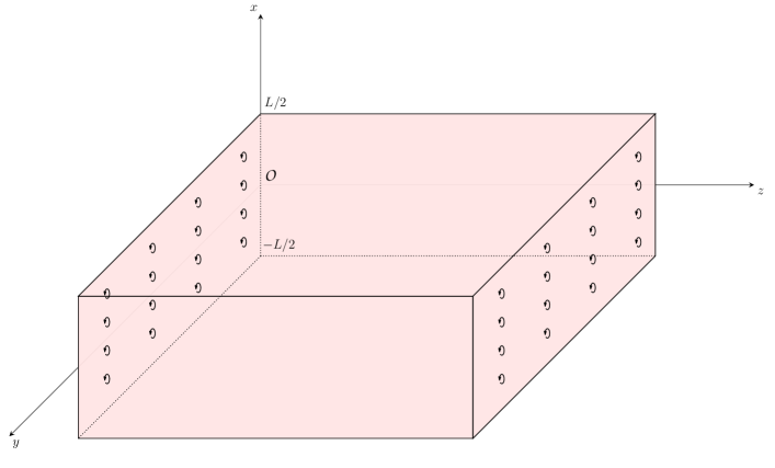
Fig. ​​​ 1: Physical setup.

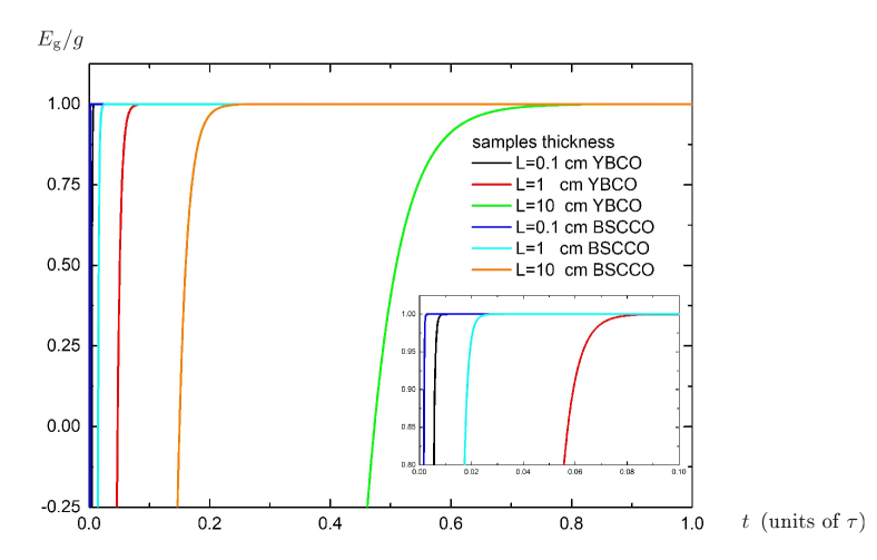
Fig. ​​​ 2: Variation of gravitational field as a function of time inside superconductive samples of YBCO (black, red and green solid line, $T=85\,\mathrm{K}$) and BSCCO (dark blue, blue and orange solid line, $T=102\,\mathrm{K}$) for different thickness values ($L=0.1\,\text{cm}$,  $L=1\,\text{cm}$,  $L=10\,\text{cm}$). In the inset, the same results are plotted in a different scale (same axes labels), to better appreciate the variations at smaller times.

	YBCO	BSCCO
$T_{\textrm{c}}$	$89\,\mathrm{K}$	$107\,\mathrm{K}$
$T_{\star}$	$85\,\mathrm{K}$	$102\,\mathrm{K}$
$\xi(T_{\star})$	$8.49\cdot 10^{-9}\,\mathrm{m}$	$4.63\cdot 10^{-9}\,\mathrm{m}$
$\lambda(T_{\star})$	$8.02\cdot 10^{-7}\,\mathrm{m}$	$1.11\cdot 10^{-6}\,\mathrm{m}$
$\sigma^{-1}$	$4.0\cdot 10^{-7}\,\Omega\,\mathrm{m}\,{}^{(\ast)}$	$3.6\cdot 10^{-6}~{}\Omega\,\mathrm{m}\,{}^{(\ast\ast)}$
$B_{\textsc{c}{}_{2}}(0)$	$61\,\mathrm{Tesla}$	$113\,\mathrm{Tesla}$
$B_{\textsc{c}{}_{2}}(T_{\star})$	$6\,\mathrm{Tesla}$	$11\,\mathrm{Tesla}$
$B_{\textsc{c}}(T_{\star})$	$0.25\,\mathrm{Tesla}$	$0.32~{}\mathrm{Tesla}$
$\lambda(0)$	$1.7\cdot 10^{-7}\,\mathrm{m}$	$2.4\cdot 10^{-7}\,\mathrm{m}$
$\xi(0)$	$1.8\cdot 10^{-9}\,\mathrm{m}$	$10^{-9}\,\mathrm{m}$
$\kappa$	$94.4$	$240.0$
$\tau(T_{\star})$	$2.01\cdot 10^{-9}\,\mathrm{s}$	$1.23\cdot 10^{-9}\,\mathrm{s}$
$\eta$	$1.0\cdot 10^{-3}$	$3.5\cdot 10^{-4}$
$\mathcal{D}$	$3.2\cdot 10^{-4}\,\mathrm{m}^{2}/\mathrm{s}$	$10^{-3}\,\mathrm{m}^{2}/\mathrm{s}$
	${}^{(\ast)}\;T\,=\,90\,\mathrm{K}$	${}^{(\ast\ast)}\;T\,=\,108\,\mathrm{K}$

Table 1: YBCO vs. BSCCO [33, 56, 57, 58]

References

- [1] Bryce S. DeWitt, “Superconductors and gravitational drag”, Phys. Rev. Lett. 16 (1966) 1092–1093.
- [2] G. Papini, “Detection of inertial effects with superconducting interferometers”, Physics Letters A 24 (1967), n. 1, 32–33.
- [3] G. Papini, “Superconducting and normal metals as detectors of gravitational waves”, Lett. Nuovo Cim. 4S1 (1970) 1027–1032.
- [4] H. Hirakawa, “Superconductors in gravitational field”, Physics Letters A 53 (1975), n. 5, 395–396.
- [5] J. Anandan, “Relativistic thermoelectromagnetic gravitational effects in normal conductors and superconductors”, Physics Letters A 105 (1984), n. 6, 280–284.
- [6] D.K. Ross, “The London equations for superconductors in a gravitational field”, Journal of Physics A: Mathematical and General 16 (1983), n. 6, 1331.
- [7] O. Yu Dinariev and A.B. Mosolov, “A relativistic effect in the theory of superconductivity”, Dokl. Akad. Nauk SSSR 295 (1987) 98.
- [8] H. Peng, “A new approach to studying local gravitomagnetic effects on a superconductor”, General Relativity and Gravitation 22 (1990), n. 6, 609–617.
- [9] H. Peng, D.G. Torr, E.K. Hu and B. Peng, “Electrodynamics of moving superconductors and superconductors under the influence of external forces”, Phys. Rev. B 43 (1991), n. 4, 2700.
- [10] H. Peng, G. Lind and Y.S. Chin, “Interaction between gravity and moving superconductors”, General relativity and gravitation 23 (1991), n. 11, 1231–1250.
- [11] Ning Li and D.G. Torr, “Effects of a gravitomagnetic field on pure superconductors”, Physical Review D 43 (1991), n. 2, 457.
- [12] E. Podkletnov and R. Nieminen, “A possibility of gravitational force shielding by bulk YBa2Cu3O7-X superconductor”, Physica C: Superconductivity 203 (1992), n. 3-4, 441–444.
- [13] E. Podkletnov, “Weak gravitation shielding properties of composite bulk YBa2Cu3O7-X superconductor below 70 K under EM field”, cond-mat/9701074 (1997).
- [14] G. Hathaway, B. Cleveland and Y. Bao, “Gravity modification experiment using a rotating superconducting disk and radio frequency fields”, Physica C: Superconductivity 385 (2003), n. 4, 488.
- [15] Ning Li, David Noever, Tony Robertson, Ron Koczor and Whitt Brantley, “Static test for a gravitational force coupled to type II YBCO superconductors”, Physica C: Superconductivity 281 (1997), n. 2, 260–267.
- [16] Giovanni Modanese, “Local contribution of a quantum condensate to the vacuum energy density”, Mod. Phys. Lett. A 18 (2003) 683–690, [gr-qc/0107073].
- [17] Giovanni Modanese, “Possible quantum gravity effects in a charged Bose condensate under variable em field”, Phys. Essays 14 (2001) 93–105, [gr-qc/9612022].
- [18] Ning Wu, “Gravitational shielding effects in gauge theory of gravity”, Commun. Theor. Phys. 41 (2004) 567–572, [hep-th/0307225].
- [19] Giovanni Modanese, “Theoretical analysis of a reported weak gravitational shielding effect”, Europhys. Lett. 35 (1996) 413–418, [hep-th/9505094].
- [20] Giovanni Modanese, “Role of a ‘local’ cosmological constant in Euclidean quantum gravity”, Phys. Rev. D 54 (1996) 5002–5009, [hep-th/9601160].
- [21] L.I. Schiff and M.V. Barnhill, “Gravitation-induced electric field near a metal”, Physical Review 151 (1966), n. 4, 1067.
- [22] A.J. Dessler, F.C. Michel, H.E. Rorschach and G.T. Trammell, “Gravitationally Induced Electric Fields in Conductors”, Phys. Rev. 168 (1968) 737–743.
- [23] Douglas G. Torr and Ning Li, “Gravitoelectric-electric coupling via superconductivity”, Foundations of Physics Letters 6 (1993), n. 4, 371–383.
- [24] Bahram Mashhoon, “Gravitoelectromagnetism”, in Reference Frames and Gravitomagnetism, pp. 121–132, World Scientific Publishing, Singapore (2000).
- [25] Bahram Mashhoon, “Gravitoelectromagnetism: A brief review”, in The Measurement of Gravitomagnetism: A Challenging Enterprise, ch. 3, pp. 29–40, Nova Science Publisher Inc., New York, USA (2007).
- [26] F.C. Witteborn and W.M. Fairbank, “Experimental comparison of the gravitational force on freely falling electrons and metallic electrons”, Physical Review Letters 19 (1967), n. 18, 1049.
- [27] F.C. Witteborn and W.M. Fairbank, “Experiments to determine the force of gravity on single electrons and positrons”, Nature 220 (1968), n. 5166, 436–440.
- [28] C. Herring, “Gravitationally induced electric field near a conductor, and its relation to the surface-stress concept”, Phys. Rev. 171 (1968), n. 5, 1361.
- [29] M. Agop, C.Gh. Buzea and P. Nica, “Local gravitoelectromagnetic effects on a superconductor”, Physica C: Superconductivity 339 (2000), n. 2, 120–128.
- [30] M. Agop, P.D. Ioannou and F. Diaconu, “Some implications of gravitational superconductivity”, Progress of Theoretical Physics 104 (2000), n. 4, 733–742.
- [31] Matteo Luca Ruggiero and Angelo Tartaglia, “Gravitomagnetic effects”, Nuovo Cim. B 117 (2002) 743–768, [gr-qc/0207065].
- [32] Angelo Tartaglia and Matteo Luca Ruggiero, “Gravitoelectromagnetism versus electromagnetism”, Eur. J. Phys. 25 (2004) 203–210, [gr-qc/0311024].
- [33] Giovanni Alberto Ummarino and Antonio Gallerati, “Superconductor in a weak static gravitational field”, Eur. Phys. J. C77 (2017), n. 8, 549, [arXiv:1710.01267].
- [34] Harihar Behera, “Comments on gravitoelectromagnetism of Ummarino and Gallerati in “Superconductor in a weak static gravitational field” vs other versions”, Eur. Phys. J. C77 (2017), n. 12, 822, [arXiv:1709.04352].
- [35] Giovanni Alberto Ummarino and Antonio Gallerati, “Exploiting weak field gravity-Maxwell symmetry in superconductive fluctuations regime”, Symmetry 11 (2019), n. 11, 1341, [arXiv:1910.13897].
- [36] Giovanni Alberto Ummarino and Antonio Gallerati, “Josephson AC effect induced by weak gravitational field”, Class. Quant. Grav. 37 (2020), n. 21, 217001, [arXiv:2009.04967].
- [37] G. A. Ummarino and A. Gallerati, “Possible alterations of local gravitational field inside a superconductor”, Entropy 23 (2021), n. 2, 193, [arXiv:2102.01489].
- [38] Antonio Gallerati, “Local affection of weak gravitational field from supercondensates”, Phys. Scripta 96 (2021), n. 6, 064001.
- [39] R. S. Vieira and H. B. Brentan, “Covariant theory of gravitation in the framework of special relativity”, Eur. Phys. J. Plus 133 (2018) 165, [arXiv:1608.00815].
- [40] Valeriy I. Sbitnev, “Quaternion algebra on 4D superfluid quantum space-time. Gravitomagnetism”, Found. Phys. 49 (2019), n. 2, 107–143, [arXiv:1901.09098].
- [41] Sergio Giardino, “A novel covariant approach to gravito-electromagnetism”, Braz. J. Phys. 50 (2020), n. 3, 372–378, [arXiv:1812.07371].
- [42] Antonio Gallerati, “Interaction between superconductors and weak gravitational field”, J. Phys. Conf. Ser. 1690 (2020), n. 1, 012141, [arXiv:2101.00418].
- [43] Q. Tang and S Wang, “Time dependent Ginzburg-Landau equations of superconductivity”, Physica D: Nonlinear Phenomena 88 (1995), n. 3-4, 139–166.
- [44] Fang-Hua Lin and Qiang Du, “Ginzburg-Landau vortices: dynamics, pinning, and hysteresis”, SIAM Journal on Mathematical Analysis 28 (1997), n. 6, 1265–1293.
- [45] S. Ullah and A.T. Dorsey, “Effect of fluctuations on the transport properties of type-ii superconductors in a magnetic field”, Physical Review B 44 (1991), n. 1, 262.
- [46] M. Ghinovker, I. Shapiro and B. Ya Shapiro, “Explosive nucleation of superconductivity in a magnetic field”, Physical Review B 59 (1999), n. 14, 9514.
- [47] N.B. Kopnin and E.V. Thuneberg, “Time-dependent Ginzburg-Landau analysis of inhomogeneous normal-superfluid transitions”, Phys. Rev. Lett. 83 (1999), n. 1, 116.
- [48] Jacqueline Fleckinger-Pellé, Hans G Kaper and Peter Takáč, “Dynamics of the Ginzburg-Landau equations of superconductivity”, Nonlinear Analysis: Theory, Methods & Applications 32 (1998), n. 5, 647–665.
- [49] Qiang Du and Paul Gray, “High-kappa limits of the time-dependent Ginzburg-Landau model”, SIAM Journal on Applied Mathematics 56 (1996), n. 4, 1060–1093.
- [50] Bakhrom Oripov and Steven M Anlage, “Time-dependent Ginzburg-Landau treatment of rf magnetic vortices in superconductors: Vortex semiloops in a spatially nonuniform magnetic field”, Phys. Rev. E 101 (2020), n. 3, 033306.
- [51] N.B. Kopnin, B.I. Ivlev and V.A. Kalatsky, “The flux-flow Hall effect in type II superconductors. An explanation of the sign reversal”, J. Low Temp. Phys. 90 (1993), n. 1, 1–13.
- [52] Nikolai Kopnin, “Theory of nonequilibrium superconductivity”; Oxford University Press, Oxford, UK (2001).
- [53] J.B. Ketterson and S.N. Song, “Superconductivity”; Cambridge University Press, Cambridge, UK (1999).
- [54] K.H. Hoffmann and Qi Tang, “Ginzburg-Landau phase transition theory and superconductivity”; Springer Basel AG, Basel, Switzerland (2012).
- [55] Jan A. Sanders, Ferdinand Verhulst and James Murdock, “Averaging methods in nonlinear dynamical systems”; Springer Verlag, New York, USA (2007).
- [56] M. Weigand, M. Eisterer, E. Giannini and H.W. Weber, “Mixed state properties of Bi2Sr2Ca2Cu3O10+δ single crystals before and after neutron irradiation”, Phys. Rev. B 81 (2010), n. 1, 014516.
- [57] A. Piriou, Y. Fasano, E. Giannini and Ø. Fischer, “Effect of oxygen-doping on Bi2Sr2Ca2Cu3O10+δ vortex matter: crossover from electromagnetic to Josephson interlayer coupling”, Phys. Rev. B 77 (2008), n. 18, 184508.
- [58] J.A. Camargo-Martínez, D. Espitia and R. Baquero, “First-principles study of electronic structure of Bi2Sr2Ca2Cu3O10”, Revista Mexicana de Física 60 (2014), n. 1, 39–45.
- [59] Anatoli Larkin and Andrei Varlamov, “Theory of fluctuations in superconductors”; Oxford University Press, Oxford, UK (2005).
- [60] J. Anandan, “Detection of gravitational radiation using superconductors”, Phys. Lett. A 110 (1985) 446–450.
- [61] W. H. Zurek, “Cosmological experiments in condensed matter systems”, Phys. Rept. 276 (1996) 177–221, [cond-mat/9607135].
- [62] T. A. Jacobson and G. E. Volovik, “Event horizons and ergoregions in He-3”, Phys. Rev. D 58 (1998) 064021, [cond-mat/9801308].
- [63] G. E. Volovik, “Superfluid analogies of cosmological phenomena”, Phys. Rept. 351 (2001) 195–348, [gr-qc/0005091].
- [64] Claus Kiefer and Carsten Weber, “On the interaction of mesoscopic quantum systems with gravity”, Annalen Phys. 14 (2005) 253–278, [gr-qc/0408010].
- [65] Stephen J. Minter, Kirk Wegter-McNelly and Raymond Y. Chiao, “Do Mirrors for Gravitational Waves Exist?”, Physica E 42 (2010) 234, [arXiv:0903.0661].
- [66] James Q. Quach, “Gravitational Casimir effect”, Phys. Rev. Lett. 114 (2015), n. 8, 081104, [arXiv:1502.07429]. [Erratum: Phys. Rev. Lett. 118 (2017) 139901].
- [67] Zaanen, Jan and Liu, Yan and Sun, Ya-Wen and Schalm, Koenraad, “Holographic duality in condensed matter physics”; Cambridge University Press, Cambridge, UK (2015).
- [68] Bijan Bagchi and Rahul Ghosh, “Dirac Hamiltonian in a supersymmetric framework”, Journal of Mathematical Physics 62 (2021), n. 7, 072101, [arXiv:2101.03922].
- [69] L. J. Garay, J. R. Anglin, J. I. Cirac and P. Zoller, “Black holes in Bose-Einstein condensates”, Phys. Rev. Lett. 85 (2000) 4643–4647, [gr-qc/0002015].
- [70] Carlos Barcelo, Stefano Liberati and Matt Visser, “Analog gravity from Bose-Einstein condensates”, Class. Quant. Grav. 18 (2001) 1137, [gr-qc/0011026].
- [71] Novello, Mario and Visser, Matt and Volovik, Grigory E., “Artificial black holes”; World Scientific, Singapore (2002).
- [72] Carlos Barcelo, Stefano Liberati and Matt Visser, “Analogue gravity”, Living Rev. Rel. 8 (2005) 12.
- [73] Iacopo Carusotto, Serena Fagnocchi, Alessio Recati, Roberto Balbinot and Alessandro Fabbri, “Numerical observation of Hawking radiation from acoustic black holes in atomic Bose-Einstein condensates”, New J. Phys. 10 (2008) 103001, [arXiv:0803.0507].
- [74] O. Boada, A. Celi, J. I. Latorre and M. Lewenstein, “Dirac Equation For Cold Atoms In Artificial Curved Spacetimes”, New J. Phys. 13 (2011) 035002, [arXiv:1010.1716].
- [75] Antonio Gallerati, “Graphene properties from curved space Dirac equation”, Eur. Phys. J. Plus 134 (2019), n. 5, 202, [arXiv:1808.01187].
- [76] Salvatore Capozziello, Richard Pincak and Emmanuel N. Saridakis, “Constructing superconductors by graphene Chern-Simons wormholes”, Annals Phys. 390 (2018) 303–333.
- [77] M. Franz and M. Rozali, “Mimicking black hole event horizons in atomic and solid-state systems”, Nature Rev. Mater. 3 (2018) 491–501, [arXiv:1808.00541].
- [78] Jiazhong Hu, Lei Feng, Zhendong Zhang and Cheng Chin, “Quantum simulation of Unruh radiation”, Nature Phys. 15 (2019), n. 8, 785–789, [arXiv:1807.07504].
- [79] Antonio Gallerati, “Negative-curvature spacetime solutions for graphene”, J. Phys. Condens. Matter 33 (2021), n. 13, 135501, [arXiv:2101.03010].
- [80] Victor I. Kolobov, Katrine Golubkov, Juan Ramón Muñoz de Nova and Jeff Steinhauer, “Observation of stationary spontaneous Hawking radiation and the time evolution of an analogue black hole”, Nature Phys. 17 (2021), n. 3, 362–367.
- [81] L. Andrianopoli, B. L. Cerchiai, R. D’Auria, A. Gallerati, R. Noris, M. Trigiante and J. Zanelli, “-extended supergravity, unconventional SUSY and graphene”, JHEP 01 (2020) 084, [arXiv:1910.03508].
- [82] A. Gallerati, “Supersymmetric theories and graphene”, PoS 390 (2021) 662, [arXiv:2104.07420].