ReGVD: Revisiting Graph Neural Networks for Vulnerability Detection

Abstract.

Identifying vulnerabilities in the source code is essential to protect the software systems from cyber security attacks. It, however, is also a challenging step that requires specialized expertise in security and code representation. To this end, we aim to develop a general, practical, and programming language-independent model capable of running on various source codes and libraries without difficulty. Therefore, we consider vulnerability detection as an inductive text classification problem and propose ReGVD, a simple yet effective graph neural network-based model for the problem. In particular, ReGVD views each raw source code as a flat sequence of tokens to build a graph, wherein node features are initialized by only the token embedding layer of a pre-trained programming language (PL) model. ReGVD then leverages residual connection among GNN layers and examines a mixture of graph-level sum and max poolings to return a graph embedding for the source code. ReGVD outperforms the existing state-of-the-art models and obtains the highest accuracy on the real-world benchmark dataset from CodeXGLUE for vulnerability detection. Our code is available at: https://github.com/daiquocnguyen/GNN-ReGVD.

1. Introduction

The software vulnerability problems have rapidly grown recently, either reported through publicly disclosed information-security flaws and exposures (CVE) or exposed inside privately-owned source codes and open-source libraries. These vulnerabilities are the main reasons for cyber security attacks on the software systems that cause substantial damages economically and socially (Neuhaus et al., 2007; Zhou et al., 2019). Therefore, vulnerability detection is an essential yet challenging step to identify vulnerabilities in the source codes to provide security solutions for the software systems.

Early approaches (Neuhaus et al., 2007; Nguyen and Tran, 2010; Shin et al., 2010) have been proposed to carefully design hand-engineered features for machine learning algorithms to detect vulnerabilities. These early approaches, however, suffer from two major drawbacks. First, creating good features requires prior knowledge, hence needs domain experts, and is usually time-consuming. Second, hand-engineered features are impractical and not straightforward to adapt to all vulnerabilities in numerous open-source codes and libraries evolving over time.

To reduce human efforts on feature engineering, some approaches (Li et al., 2018; Russell et al., 2018) consider each raw source code as a flat natural language sequence and explore deep learning architectures applied for natural language processing (NLP) (such as LSTMs (Hochreiter and Schmidhuber, 1997) and CNNs (Kim, 2014)) in detecting vulnerabilities. Recently, pre-trained language models such as BERT (Devlin et al., 2018) have emerged as a trending learning paradigm, achieving significant success in NLP applications. Inspired by this BERT-style trending paradigm, pre-trained programming language (PL) models such as CodeBERT (Feng et al., 2020) have improved the performance of PL downstream tasks such as vulnerability detection. However, as mentioned in (Nguyen et al., 2019), all interactions among all positions in the input sequence inside the self-attention layer of the BERT-style model build up a complete graph, i.e., every position has an edge to all other positions; thus, this limits learning local structures within the source code to differentiate vulnerabilities.

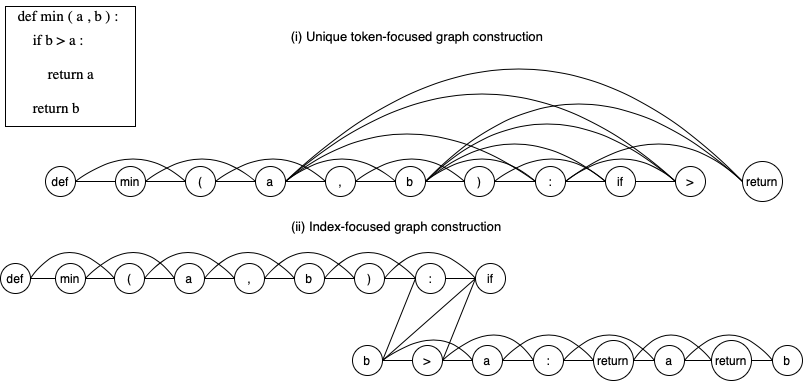
Figure 1. An illustration for two graph construction methods with a fixed-size sliding window of length 3.

Graph neural networks (GNNs) have recently become a primary method to embed nodes and graphs into low-dimensional continuous vector spaces (Hamilton et al., 2017; Wu et al., 2019; Nguyen, 2021). GNNs provide faster and practical training, higher accuracy, and state-of-the-art results for downstream tasks such as text classification (Yao et al., 2019; Huang et al., 2019; Zhang et al., 2020; Nguyen et al., 2021). Devign (Zhou et al., 2019) is proposed to utilize Gated GNNs (Li et al., 2016) for vulnerability detection, wherein Devign uses a PL parser to extract multi-edged graph information. However, Devign is difficult of being practiced in reality. The main reason is that there is not a perfect parser in reality for each PL, which can successfully parse a variety of source codes and libraries without any internal compile errors and exceptions.

In this paper, our goal is to develop a general, practical, and programming language-independent model capable of running on various source codes and libraries without difficulty. Hence, we consider vulnerability detection as an inductive text classification problem and introduce ReGVD – a simple yet effective GNN-based model for vulnerability detection as follows: (i) ReGVD views each raw source code as a flat sequence of tokens to construct a graph (in Section 2.2), wherein node features are initialized by only the token embedding layer of a pre-trained PL model. (ii) ReGVD leverages GNNs (such as GCNs (Kipf and Welling, 2017) or Gated GNNs (Li et al., 2016)) using residual connection among GNN layers (in Section 2.3). (iii) ReGVD examines a mixture between the sum and max poolings to produce a graph embedding for the source code (in Section 2.4). This graph embedding is fed to a single fully-connected layer followed by a softmax layer to predict the code vulnerabilities. Extensive experiments show that ReGVD significantly outperforms the existing state-of-the-art models on the benchmark vulnerability detection dataset from CodeXGLUE (Lu et al., 2021). ReGVD produces the highest accuracy of 63.69%, gaining absolute improvements of 1.61% and 1.39% over CodeBERT and GraphCodeBERT, respectively; thus, ReGVD can act as a new strong baseline for future work.

2. The proposed ReGVD

2.1. Problem definition

We consider vulnerability detection for source code at the function level, i.e., we aim to identify whether a given function in raw source code is vulnerable or not (Zhou et al., 2019). We define a data sample as $\left\{(\mathsf{c}_{i},\mathsf{y}_{i})|\mathsf{c}_{i}\in\mathbb{C},\mathsf{y}_{i}\in\mathbb{Y}\right\}_{i=1}^{n}$, where $\mathbb{C}$ represents the set of raw source codes, $\mathbb{Y}=\{0,1\}$ denotes the label set with $1$ for vulnerable and $0$ otherwise, and $n$ is the number of instances. In this work, we consider vulnerability detection as an inductive text classification problem and leverage GNNs for the problem. Therefore, we construct a graph $\mathsf{g}_{i}(\mathcal{V},\boldsymbol{X},\boldsymbol{A})\in\mathcal{G}$ for each source code $\mathsf{c}_{i}$, wherein $\mathcal{V}$ is a set of $m$ nodes in the graph; $\boldsymbol{X}\in\mathbb{R}^{m\times d}$ is the node feature matrix, wherein each node $\mathsf{v}_{j}\in\mathcal{V}$ is represented by a $d$-dimensional real-valued vector $\boldsymbol{x}_{j}\in\mathbb{R}^{d}$; $\boldsymbol{A}\in\{0,1\}^{m\times m}$ is the adjacency matrix, where $\boldsymbol{A}_{\mathsf{v},\mathsf{u}}$ equal to 1 means having an edge between node $\mathsf{v}$ and node $\mathsf{u}$, and 0 otherwise. We aim to learn a mapping function $f:\mathcal{G}\rightarrow\mathbb{Y}$ to determine whether a given source code is vulnerable or not. The mapping function $f$ can be learned by minimizing the loss function with the regularization on model parameters $\boldsymbol{\theta}$ as:

$$\mathsf{min}\sum_{i=1}^{n}\mathcal{L}(f(\mathsf{g}_{i}(\mathcal{V},\boldsymbol{X},\boldsymbol{A}),\mathsf{y}_{i}|\mathsf{c}_{i}))+\lambda\|\boldsymbol{\theta}\|_{2}^{2}$$

where $\mathcal{L}(.)$ is the cross-entropy loss function and and $\lambda$ is an adjustable weight.

2.2. Graph construction

We consider a raw source code as a flat sequence of tokens and illustrate two graph construction methods (Huang et al., 2019; Zhang et al., 2020) in Figure 1, wherein we omit self-loops in these two methods since the self-loops do not help to improve performance in our pilot experiments.

Unique token-focused construction

We represent unique tokens as nodes and co-occurrences between tokens (within a fixed-size sliding window) as edges, and the obtained graph has an adjacency matrix $\boldsymbol{A}$ as:

$$\boldsymbol{A}_{\mathsf{v},\mathsf{u}}=\left\{\begin{array}[]{l}1\ \ \ \text{If $\mathsf{v}$ and $\mathsf{u}$ co-occur within a sliding window}\\ \ \ \ \ \ \ \ \ \ \ \text{and $\mathsf{v}\neq\mathsf{u}$.}\\ 0\ \ \ \text{Otherwise.}\end{array}\right.$$

Index-focused construction

Given a flat sequence of $l$ tokens $\left\{t_{\mathsf{i}}\right\}_{\mathsf{i}=1}^{l}$, we represent all tokens as the nodes, i.e., treating each index $\mathsf{i}$ as a node to represent token $t_{\mathsf{i}}$. The number of nodes equals the sequence length. We also consider co-occurrences between indexes (within a fixed-size sliding window) as edges, and the obtained graph has an adjacency matrix $\boldsymbol{A}$ as:

$$\boldsymbol{A}_{\mathsf{i},\mathsf{j}}=\left\{\begin{array}[]{l}1\ \ \ \text{If $\mathsf{i}$ and $\mathsf{j}$ co-occur within a sliding window}\\ \ \ \ \ \ \ \ \ \ \ \text{and $\mathsf{i}\neq\mathsf{j}$.}\\ 0\ \ \ \text{Otherwise.}\end{array}\right.$$

Node feature initialization

It is worth noting that pre-trained programming language (PL) models such as CodeBERT (Feng et al., 2020) have recently improved the performance of PL downstream tasks such as vulnerability detection. To attain the advantage of the pre-trained PL model and also to make a fair comparison, we use only the token embedding layer of the pre-trained PL model to initialize node feature vectors for reporting our final results.

2.3. Graph neural networks with residual connection

GNNs aim to update vector representations of nodes by recursively aggregating vector representations from their neighbours (Scarselli et al., 2009; Kipf and Welling, 2017). Mathematically, given a graph $\mathsf{g}(\mathcal{V},\boldsymbol{X},\boldsymbol{A})$, we simply formulate GNNs as follows:

$$\boldsymbol{\mathsf{H}}^{(k+1)}=\mathsf{GNN}\left(\boldsymbol{A},\boldsymbol{\mathsf{H}}^{(k)}\right)$$

where $\boldsymbol{\mathsf{H}}^{(k)}$ is the matrix representation of nodes at the $k$-th iteration/layer; and $\boldsymbol{\mathsf{H}}^{(0)}=\boldsymbol{X}$. There have been many GNNs proposed in recent literature (Wu et al., 2019), wherein Graph Convolutional Networks (GCNs) (Kipf and Welling, 2017) is the most widely-used one, and Gated graph neural networks (“Gated GNNs” or “GGNNs” for short) (Li et al., 2016) is also suitable for our data structure. Our ReGVD leverages GCNs and GGNNs as the base models.

Formally, GCNs is given as follows:

$$\boldsymbol{\mathsf{h}}_{\mathsf{v}}^{(k+1)}=\phi\left(\sum_{\mathsf{u}\in\mathcal{N}_{\mathsf{v}}}a_{\mathsf{v},\mathsf{u}}\boldsymbol{W}^{(k)}\boldsymbol{\mathsf{h}}_{\mathsf{u}}^{(k)}\right),\forall\mathsf{v}\in\mathcal{V}$$

where $a_{\mathsf{v},\mathsf{u}}$ is an edge constant between nodes $\mathsf{v}$ and $\mathsf{u}$ in the Laplacian re-normalized adjacency matrix $\textbf{D}^{-\frac{1}{2}}\boldsymbol{A}\textbf{D}^{-\frac{1}{2}}$ (as we omit self-loops), wherein D is the diagonal node degree matrix of $\boldsymbol{A}$; $\boldsymbol{W}^{(k)}$ is a weight matrix; and $\phi$ is a nonlinear activation function such as $\mathsf{ReLU}$.

GGNNs adopts GRUs (Cho et al., 2014), unrolls the recurrence for a fixed number of timesteps, and removes the need to constrain parameters to ensure convergence as:

$$\textbf{a}_{\mathsf{v}}^{(k+1)} = \sum_{\mathsf{u}\in\mathcal{N}_{\mathsf{v}}}a_{\mathsf{v},\mathsf{u}}\boldsymbol{\mathsf{h}}_{\mathsf{u}}^{(k)}$$

$$\textbf{z}_{\mathsf{v}}^{(k+1)} = \sigma\left(\textbf{W}^{z}\textbf{a}_{\mathsf{v}}^{(k+1)}+\textbf{U}^{z}\boldsymbol{\mathsf{h}}_{\mathsf{v}}^{(k)}\right)$$

$$\textbf{r}_{\mathsf{v}}^{(k+1)} = \sigma\left(\textbf{W}^{r}\textbf{a}_{\mathsf{v}}^{(k+1)}+\textbf{U}^{r}\boldsymbol{\mathsf{h}}_{\mathsf{v}}^{(k)}\right)$$

$$\widetilde{\boldsymbol{\mathsf{h}}_{\mathsf{v}}^{(k+1)}} = \phi\left(\textbf{W}^{o}\textbf{a}_{\mathsf{v}}^{(k+1)}+\textbf{U}^{o}\left(\textbf{r}_{\mathsf{v}}^{(k+1)}\odot\boldsymbol{\mathsf{h}}_{\mathsf{v}}^{(k)}\right)\right)$$

$$\boldsymbol{\mathsf{h}}_{\mathsf{v}}^{(k+1)} = \left(1-\textbf{z}_{\mathsf{v}}^{(k+1)}\right)\odot\boldsymbol{\mathsf{h}}_{\mathsf{v}}^{(k)}+\textbf{z}_{\mathsf{v}}^{(k+1)}\odot\widetilde{\boldsymbol{\mathsf{h}}_{\mathsf{v}}^{(k+1)}}$$

where z and r are the update and reset gates; $\sigma$ is the sigmoid function; and $\odot$ is the element-wise multiplication.

The residual connection (He et al., 2016) is used to incorporate information learned in the lower layers to the higher layers, and more importantly, to allow gradients to directly pass through the layers to avoid vanishing gradient or exploding gradient problems. Motivated by that, we follow (Bresson and Laurent, 2017) to adapt residual connection among the GNN layers, with fixing the same hidden size for the different layers. In particular, ReGVD redefines GNNs as:

$$\boldsymbol{\mathsf{H}}^{(k+1)}=\boldsymbol{\mathsf{H}}^{(k)}+\mathsf{GNN}\left(\boldsymbol{A},\boldsymbol{\mathsf{H}}^{(k)}\right)$$

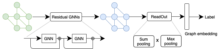
Figure 2. An illustration for our proposed ReGVD.

2.4. Graph-level readout pooling layer

The graph-level readout layer is used to produce a graph embedding for each input graph. ReGVD leverages the sum pooling as it produces better results for graph classification (Xu et al., 2019). Besides, ReGVD utilizes the max pooling to exploit more information on the node representations. ReGVD then considers a mixture between the sum and max poolings to produce the graph embedding $\boldsymbol{\mathsf{e}}_{\mathsf{g}}$ as:

$$\boldsymbol{\mathsf{e}}_{\mathsf{v}} = \sigma\left(\textbf{w}^{\mathsf{T}}\boldsymbol{\mathsf{h}}_{\mathsf{v}}^{(K)}+\mathsf{b}\right)\odot\phi\left(\textbf{W}\boldsymbol{\mathsf{h}}_{\mathsf{v}}^{(K)}+\boldsymbol{\mathsf{b}}\right)$$

$$\boldsymbol{\mathsf{e}}_{\mathsf{g}} = \mathsf{MIX}\left(\sum_{\mathsf{v}\in\mathcal{V}}\boldsymbol{\mathsf{e}}_{\mathsf{v}},\textsc{MaxPool}\left\{\boldsymbol{\mathsf{e}}_{\mathsf{v}}\right\}_{\mathsf{v}\in\mathcal{V}}\right)$$

where $\boldsymbol{\mathsf{e}}_{\mathsf{v}}$ is the final vector representation of node $\mathsf{v}$, wherein $\sigma\left(\textbf{w}^{\mathsf{T}}\boldsymbol{\mathsf{h}}_{\mathsf{v}}^{(K)}+\mathsf{b}\right)$ acts as soft attention mechanisms over nodes (Li et al., 2016), and $\boldsymbol{\mathsf{h}}_{\mathsf{v}}^{(K)}$ is the vector representation of node $\mathsf{v}$ at the last $K$-th layer; and $\mathsf{MIX}(.)$ denotes an arbitrary function. ReGVD examines three $\mathsf{MIX}$ functions consisting of $\mathsf{SUM}$, $\mathsf{MUL}$, and $\mathsf{CONCAT}$ as:

$$\mathsf{SUM} : \boldsymbol{\mathsf{e}}_{\mathsf{g}}=\sum_{\mathsf{v}\in\mathcal{V}}\boldsymbol{\mathsf{e}}_{\mathsf{v}}+\textsc{MaxPool}\left\{\boldsymbol{\mathsf{e}}_{\mathsf{v}}\right\}_{\mathsf{v}\in\mathcal{V}}$$

$$\mathsf{MUL} : \boldsymbol{\mathsf{e}}_{\mathsf{g}}=\sum_{\mathsf{v}\in\mathcal{V}}\boldsymbol{\mathsf{e}}_{\mathsf{v}}\odot\textsc{MaxPool}\left\{\boldsymbol{\mathsf{e}}_{\mathsf{v}}\right\}_{\mathsf{v}\in\mathcal{V}}$$

$$\mathsf{CONCAT} : \boldsymbol{\mathsf{e}}_{\mathsf{g}}=\left[\sum_{\mathsf{v}\in\mathcal{V}}\boldsymbol{\mathsf{e}}_{\mathsf{v}}\ \ \ \|\ \ \ \textsc{MaxPool}\left\{\boldsymbol{\mathsf{e}}_{\mathsf{v}}\right\}_{\mathsf{v}\in\mathcal{V}}\right]$$

After that, ReGVD feeds $\boldsymbol{\mathsf{e}}_{\mathsf{g}}$ to a single fully-connected layer followed by a $\mathsf{softmax}$ layer to predict whether the source code is vulnerable or not as: $\boldsymbol{\mathsf{\hat{y}}}_{\mathsf{g}}=\mathsf{softmax}\left(\textbf{W}_{1}\boldsymbol{\mathsf{e}}_{\mathsf{g}}+\textbf{b}_{1}\right)$ Finally, ReGVD is trained by minimizing the cross-entropy loss function as mentioned in Section 2.1. We illustrate the proposed ReGVD in Figure 2.

3. Experimental setup and results

3.1. Experimental setup

Dataset

We use the real-world benchmark from CodeXGLUE (Lu et al., 2021) for vulnerability detection at the function level. The dataset was firstly created by Zhou et al. (2019), including 27,318 manually-labeled vulnerable or non-vulnerable functions extracted from security-related commits in two large and popular C programming language open-source projects (i.e., QEMU and FFmpeg) and diversified in functionality. Then Lu et al. (2021) combined these projects and then split into the training/validation/test sets.

Training protocol

We construct a 2-layer model, set the batch size to 128, and employ the Adam optimizer (Kingma and Ba, 2014) to train our model up to 100 epochs. As mentioned in Section 2.3, we set the same hidden size (“hs”) for the hidden GNN layers, wherein we vary the size value in {128, 256, 384}. We vary the sliding window size (“ws”) in {2, 3, 4, 5} and the Adam initial learning rate (“lr”) in $\left\{1e^{-4},5e^{-4},1e^{-3}\right\}$. The final accuracy on the test set is reported for the best model checkpoint, which obtains the highest accuracy on the validation set.

Baselines

We compare our ReGVD with strong and up-to-date baselines as follows:

• BiLSTM (Hochreiter and Schmidhuber, 1997) and TextCNN (Kim, 2014) are two well-known standard models applied for text classification.

• RoBERTa (Liu et al., 2019) is built based on BERT (Devlin et al., 2018) by removing the next-sentence objective and training on a massive dataset with larger mini-batches and learning rates.

• Devign (Zhou et al., 2019) builds a multi-edged graph from a raw source code, then uses Gated GNNs (Li et al., 2016) to update node representations, and finally utilizes a 1-D CNN-based pooling (“Conv”) to make a prediction. We note that Zhou et al. (2019) did not release the official implementation of Devign. Thus, we re-implement Devign using the same training and evaluation protocols.

• CodeBERT (Feng et al., 2020) is a pre-trained model also based on BERT for 6 programming languages (Python, Java, JavaScript, PHP, Ruby, Go), using masked language model (Devlin et al., 2018) and replaced token detection (Clark et al., 2020) objectives.

• GraphCodeBERT (Guo et al., 2021) is a new pre-trained PL model, extending CodeBERT to consider the inherent structure of code data flow into the training objective.

3.2. Main results

Table 1. Vulnerability detection accuracies (%) on the test set. The best scores are in bold, while the second best scores are in underline. The results of BiLSTM, TextCNN, RoBERTa, and CodeBERT are taken from (Lu et al., 2021). $\star$ denotes that we report our own results for other baselines. “Idx” and “UniT” denote the index-focused graph construction and the unique token-focused one, respectively. “CB” and “G-CB” denote using only the token embedding layer of CodeBERT and GraphCodeBERT to initialize the node features, respectively.

Model	Accuracy
BiLSTM	59.37
TextCNN	60.69
RoBERTa	61.05
CodeBERT	62.08
GraphCodeBERT⋆	62.30
Devign (Idx + CB)⋆	60.43
Devign (Idx + G-CB)⋆	61.31
Devign (UniT + CB)⋆	60.40
Devign (UniT + G-CB)⋆	59.77
ReGVD (GGNN + Idx + CB)	63.54
ReGVD (GGNN + Idx + G-CB)	63.29
ReGVD (GGNN + UniT + CB)	63.62
ReGVD (GGNN + UniT + G-CB)	62.41
ReGVD (GCN + Idx + CB)	62.63
ReGVD (GCN + Idx + G-CB)	62.70
ReGVD (GCN + UniT + CB)	63.14
ReGVD (GCN + UniT + G-CB)	63.69

Table 1 presents the accuracy results of the proposed ReGVD and the strong and up-to-date baselines on the real-world benchmark dataset from CodeXGLUE for vulnerability detection. We note that both the recent models CodeBERT and GraphCodeBERT obtain competitive performances and perform better than Devign, indicating the effectiveness of the pre-trained PL models. More importantly, ReGVD gains absolute improvements of 1.61% and 1.39% over CodeBERT and GraphCodeBERT, respectively. This shows the benefit of ReGVD in learning the local structures inside the source code to differentiate vulnerabilities (w.r.t using only the token embedding layer of the pre-trained PL model). Hence, our ReGVD significantly outperforms the up-to-date baseline models. In particular, ReGVD produces the highest accuracy of 63.69% – a new state-of-the-art result on the CodeXGLUE vulnerability detection dataset.

We look at Figure 3(a) to investigate whether the graph-level readout layer proposed in ReGVD performs better than the Conv pooling layer utilized in Devign. Since Devign also uses Gated GNNs to update the node representations and gains the best accuracy of 61.31% for the setting (Idx+G-CB); thus, we consider the ReGVD setting (GGNN+Idx +G-CB) without using the residual connection for a fair comparison, wherein ReGVD achieves an accuracy of 63.51%, which is 2.20% higher accuracy than that of Devign. More generally, we get a similar conclusion from the results of three remaining ReGVD settings (without using the residual connection) that the graph-level readout layer utilized in ReGVD outperforms that used in Devign.

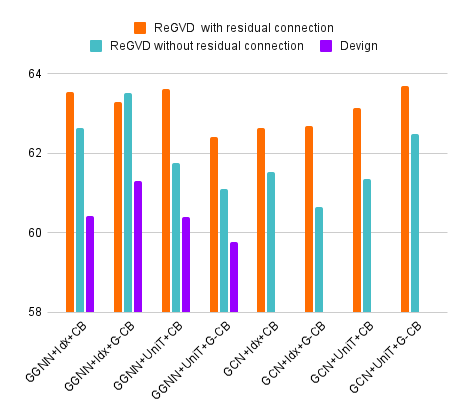
(a) Accuracy with and without residual connection.

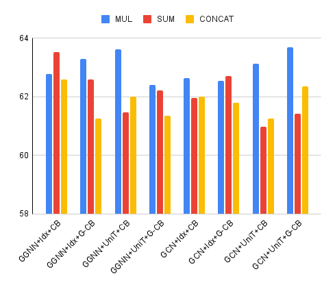
(b) Accuracy w.r.t the $\mathsf{MIX}$ functions.

Figure 3. Accuracy with different settings.

We analyze the influence of the residual connection and the mixture function. We first look back Figure 3(a) for the ReGVD accuracies w.r.t with and without using the residual connection among the GNN layers. It demonstrates that the residual connection helps to boost the GNNs performance on seven settings, where the maximum accuracy gain is 2.05% for the ReGVD setting (GCN+Idx+G-CB). Next, we look at Figure 3(b) for the ReGVD results w.r.t the $\mathsf{MIX}$ functions. We find that ReGVD generally gains the highest accuracies on six settings using the $\mathsf{MUL}$ operator and on two remaining settings using the $\mathsf{SUM}$ operator. But it is worth noting that the ReGVD setting (GGNN+Idx+CB) using the $\mathsf{CONCAT}$ operator obtains an accuracy of 62.59%, which is still higher than that of Devign, CodeBERT, and GraphCodeBERT.

Furthermore, our model achieves satisfactory performance with limited training data, compared to the baselines using the full training data. For example, ReGVD obtains an accuracy of 61.68% with 60% training set, which is higher than the accuracies of BiLSTM, TextCNN, RoBERTa, and Devign. It also achieves an accuracy of 62.55% with 80% training set, which is better than those of CodeBERT and GraphCodeBERT.

4. Conclusion

We consider vulnerability identification as an inductive text classification problem and introduce a simple yet effective graph neural network-based model, named ReGVD, to detect vulnerabilities in source code. ReGVD transforms each raw source code into a graph, wherein ReGVD utilizes only the token embedding layer of the pre-trained programming language model to initialize node feature vectors. ReGVD then leverages residual connection among GNN layers and a mixture of the sum and max poolings to learn graph representation. To demonstrate the effectiveness of ReGVD, we conduct extensive experiments to compare ReGVD with the strong and up-to-date baselines on the benchmark vulnerability detection dataset from CodeXGLUE. Experimental results show that the proposed ReGVD is significantly better than the baseline models and obtains the highest accuracy of 63.69% on the benchmark dataset. ReGVD can be seen as a general, practical, and programming language-independent model that can run on various source codes and libraries without difficulty.

References

- (1)
- Bresson and Laurent (2017) Xavier Bresson and Thomas Laurent. 2017. Residual gated graph convnets. arXiv preprint arXiv:1711.07553 (2017).
- Cho et al. (2014) Kyunghyun Cho, Bart van Merriënboer, Caglar Gulcehre, Dzmitry Bahdanau, Fethi Bougares, Holger Schwenk, and Yoshua Bengio. 2014. Learning Phrase Representations using RNN Encoder–Decoder for Statistical Machine Translation. In EMNLP. 1724––1734.
- Clark et al. (2020) Kevin Clark, Minh-Thang Luong, Quoc V Le, and Christopher D Manning. 2020. Electra: Pre-training text encoders as discriminators rather than generators. arXiv preprint arXiv:2003.10555 (2020).
- Devlin et al. (2018) Jacob Devlin, Ming-Wei Chang, Kenton Lee, and Kristina Toutanova. 2018. Bert: Pre-training of deep bidirectional transformers for language understanding. arXiv preprint arXiv:1810.04805 (2018).
- Feng et al. (2020) Zhangyin Feng, Daya Guo, Duyu Tang, Nan Duan, Xiaocheng Feng, Ming Gong, Linjun Shou, Bing Qin, Ting Liu, Daxin Jiang, and Ming Zhou. 2020. CodeBERT: A Pre-Trained Model for Programming and Natural Languages. In Findings of the Association for Computational Linguistics: EMNLP 2020. 1536–1547.
- Guo et al. (2021) Daya Guo, Shuo Ren, Shuai Lu, Zhangyin Feng, Duyu Tang, Shujie Liu, Long Zhou, Nan Duan, Alexey Svyatkovskiy, Shengyu Fu, Michele Tufano, Shao Kun Deng, Colin B. Clement, Dawn Drain, Neel Sundaresan, Jian Yin, Daxin Jiang, and Ming Zhou. 2021. GraphCodeBERT: Pre-training Code Representations with Data Flow. In ICLR.
- Hamilton et al. (2017) William L. Hamilton, Rex Ying, and Jure Leskovec. 2017. Representation learning on graphs: Methods and applications. preprint arXiv:1709.05584 (2017).
- He et al. (2016) Kaiming He, Xiangyu Zhang, Shaoqing Ren, and Jian Sun. 2016. Deep residual learning for image recognition. In CVPR. 770–778.
- Hochreiter and Schmidhuber (1997) Sepp Hochreiter and Jürgen Schmidhuber. 1997. Long Short-Term Memory. Neural Computation 9 (1997), 1735–1780.
- Huang et al. (2019) Lianzhe Huang, Dehong Ma, Sujian Li, Xiaodong Zhang, and Houfeng Wang. 2019. Text Level Graph Neural Network for Text Classification. In EMNLP-IJCNLP.
- Kim (2014) Yoon Kim. 2014. Convolutional Neural Networks for Sentence Classification. In EMNLP. 1746–1751.
- Kingma and Ba (2014) Diederik Kingma and Jimmy Ba. 2014. Adam: A Method for Stochastic Optimization. arXiv preprint arXiv:1412.6980 (2014).
- Kipf and Welling (2017) Thomas N. Kipf and Max Welling. 2017. Semi-Supervised Classification with Graph Convolutional Networks. In ICLR.
- Li et al. (2016) Yujia Li, Daniel Tarlow, Marc Brockschmidt, and Richard Zemel. 2016. Gated Graph Sequence Neural Networks. In ICLR.
- Li et al. (2018) Zhen Li, Deqing Zou, Shouhuai Xu, Xinyu Ou, Hai Jin, Sujuan Wang, Zhijun Deng, and Yuyi Zhong. 2018. Vuldeepecker: A deep learning-based system for vulnerability detection. arXiv preprint arXiv:1801.01681 (2018).
- Liu et al. (2019) Yinhan Liu, Myle Ott, Naman Goyal, Jingfei Du, Mandar Joshi, Danqi Chen, Omer Levy, Mike Lewis, Luke Zettlemoyer, and Veselin Stoyanov. 2019. Roberta: A robustly optimized bert pretraining approach. arXiv preprint arXiv:1907.11692 (2019).
- Lu et al. (2021) Shuai Lu, Daya Guo, Shuo Ren, Junjie Huang, Alexey Svyatkovskiy, Ambrosio Blanco, Colin B. Clement, Dawn Drain, Daxin Jiang, Duyu Tang, Ge Li, Lidong Zhou, Linjun Shou, Long Zhou, Michele Tufano, Ming Gong, Ming Zhou, Nan Duan, Neel Sundaresan, Shao Kun Deng, Shengyu Fu, and Shujie Liu. 2021. CodeXGLUE: A Machine Learning Benchmark Dataset for Code Understanding and Generation. arXiv preprint arXiv:2102.04664 (2021).
- Neuhaus et al. (2007) Stephan Neuhaus, Thomas Zimmermann, Christian Holler, and Andreas Zeller. 2007. Predicting vulnerable software components. In ACM CCS. 529–540.
- Nguyen (2021) Dai Quoc Nguyen. 2021. Representation Learning for Graph-Structured Data. Ph.D. Dissertation. Monash University. https://doi.org/10.26180/14450496.v1
- Nguyen et al. (2019) Dai Quoc Nguyen, Tu Dinh Nguyen, and Dinh Phung. 2019. Universal Graph Transformer Self-Attention Networks. arXiv preprint arXiv:1909.11855 (2019).
- Nguyen et al. (2021) Dai Quoc Nguyen, Tu Dinh Nguyen, and Dinh Phung. 2021. Quaternion Graph Neural Networks. In Asian Conference on Machine Learning.
- Nguyen and Tran (2010) Viet Hung Nguyen and Le Minh Sang Tran. 2010. Predicting vulnerable software components with dependency graphs. In MetriSec. 1–8.
- Russell et al. (2018) Rebecca Russell, Louis Kim, Lei Hamilton, Tomo Lazovich, Jacob Harer, Onur Ozdemir, Paul Ellingwood, and Marc McConley. 2018. Automated vulnerability detection in source code using deep representation learning. In ICMLA.
- Scarselli et al. (2009) Franco Scarselli, Marco Gori, Ah Chung Tsoi, Markus Hagenbuchner, and Gabriele Monfardini. 2009. The graph neural network model. IEEE Transactions on Neural Networks 20 (2009), 61–80.
- Shin et al. (2010) Yonghee Shin, Andrew Meneely, Laurie Williams, and Jason A Osborne. 2010. Evaluating complexity, code churn, and developer activity metrics as indicators of software vulnerabilities. IEEE transactions on software engineering 37 (2010).
- Wu et al. (2019) Zonghan Wu, Shirui Pan, Fengwen Chen, Guodong Long, Chengqi Zhang, and Philip S Yu. 2019. A comprehensive survey on graph neural networks. arXiv:1901.00596.
- Xu et al. (2019) Keyulu Xu, Weihua Hu, Jure Leskovec, and Stefanie Jegelka. 2019. How Powerful Are Graph Neural Networks?. In ICLR.
- Yao et al. (2019) Liang Yao, Chengsheng Mao, and Yuan Luo. 2019. Graph convolutional networks for text classification. In AAAI. 7370–7377.
- Zhang et al. (2020) Yufeng Zhang, Xueli Yu, Zeyu Cui, Shu Wu, Zhongzhen Wen, and Liang Wang. 2020. Every Document Owns Its Structure: Inductive Text Classification via Graph Neural Networks. In ACL. 334–339.
- Zhou et al. (2019) Yaqin Zhou, Shangqing Liu, Jingkai Siow, Xiaoning Du, and Yang Liu. 2019. Devign: Effective Vulnerability Identification by Learning Comprehensive Program Semantics via Graph Neural Networks. In NeurIPS.