Sama Daryanavard, University of Glasgow, Glasgow G12 8QQ, UK.
- GSV
- Grey-Scale Value
- RPi
- Raspberry Pi 3B+
- Control Error
- LDR
- Light Dependent Resistor
- MC
- Motor Command
- FIR
- Finite Impulse Response
- FA
- Filter Array
- FoV
- Field of View
- G
- Grey Value
- SaR
- Sign and Relevance
- LTP
- Long-Term Potentiation
- LTD
- Long-Term Depression
- GDM
- Gradient Descent Method
Sign and relevance learning
Abstract
Standard models of biologically realistic or biologically inspired reinforcement learning employ a global error signal, which implies the use of shallow networks. On the other hand, error backpropagation allows the use of networks with multiple layers. However, precise error backpropagation is difficult to justify in biologically realistic networks because it requires precise weighted error backpropagation from layer to layer. In this study, we introduce a novel network that solves this problem by propagating only the sign of the plasticity change (i.e., LTP/LTD) throughout the whole network, while neuromodulation controls the learning rate. Neuromodulation can be understood as a rectified error or relevance signal, while the top-down sign of the error signal determines whether long-term potentiation or long-term depression will occur. To demonstrate the effectiveness of this approach, we conducted a real robotic task as proof of concept. Our results show that this paradigm can successfully perform complex tasks using a biologically plausible learning mechanism.
keywords:
neuromodulation, reinforcement learning, deep learning, synaptic plasticity, dopamine, serotonin1 Introduction
The learning of an organism can be understood in the context of its interactions with the environment, facilitated through sensory inputs and motor outputs, which, in turn, lead to new sensory inputs (Maffei et al., 2017). The framework for such learning is based on closed-loop learning (von Uexküll, 1926), where actions result in either positive or negative consequences. This is the realm of reinforcement learning (Dayan and Balleine, 2002). The reward prediction error is central to reinforcement learning in a biologically realistic framework. In the 1990s, Schultz et al. (1997) suggested that dopamine codes this error (Bromberg-Martin et al., 2010; Wood et al., 2017; Takahashi et al., 2017), which is similar to the temporal difference error in machine learning (Sutton, 1988). This led to the assumption that the brain resembles an actor/critic architecture, where dopamine, as the reward prediction error, drives synaptic changes in the striatum (Humphries et al., 2006). Another interpretation of the actor/critic architecture is that it represents a nested closed-loop platform, where an inner reflex loop generates an error signal that tunes an actor in an outer loop to create anticipatory actions. In other words, the actor generates a forward model of the reflex (Porr and Wörgötter, 2002). Therefore, the actor/critic architecture can be used for both model-based (Verschure and Coolen, 1991b) and model-free learning.
However, relying solely on a global error signal, such as the dopamine reward prediction error, has its limitations as this error signal affects all neurons (Humphries et al., 2006; O’Reilly and Frank, 2006), thus making multi-layer networks less useful. For this reason, while the striatum may be a single-layer structure that receives dopamine from the substantia nigra pars compacta (SNc), cortical networks, such as the orbitofrontal (OFC) and medial prefrontal cortices (mPFC), are also heavily involved in reinforcement learning and decision making (Haber et al., 1995; Berthoud, 2004; Rolls and Grabenhorst, 2008; Dela Cruz et al., 2016), being innervated by dopaminergic neurons from the ventral tegmental area (VTA).
In the context of cortical pyramidal neurons, it is important to remember that the main method by which plasticity is induced is through learning rules such as Hebbian learning (Hebb, 1949; Bliss and Lomo, 1973) or spike-timing-dependent plasticity (STDP) (Markram et al., 1997), with its underlying postsynaptic calcium dynamics where a high concentration causes Long-Term Potentiation (LTP) and a low concentration causes Long-Term Depression (LTD) (Lu et al., 2001; Castellani et al., 2001). Therefore, calcium determines the sign of the plasticity, whether it is LTP or LTD. These learning rules interact with the global neuromodulator (Mattson et al., 2004; Lovinger, 2010), particularly serotonin (Roberts, 2011; Linley et al., 2013; Luo et al., 2015; Li et al., 2016; Crockett et al., 2009), but also dopamine (Dela Cruz et al., 2016), which can be thought of as controlling the overall learning rate. From a theoretical point of view, this has inspired ISO3 learning, where differential Hebb is combined with a rectified error signal called “relevance”. Nonetheless, this network is also shallow, consisting of just one layer.
This paper presents a novel learning mechanism that expands upon the single-layer approach of ISO3 learning (Porr and Wörgötter, 2007a) by incorporating multiple layers. Our network utilises a top-down pass of the sign of an error signal to determine whether to implement LTP or LTD, while a global neuromodulator controls the learning speed. As a proof of concept, we apply our mechanism to a simple line-following task on a real robot. The robot’s deviation generates an error signal that is used to train the network.
2 The Sign and Relevance (SaR) learning platform
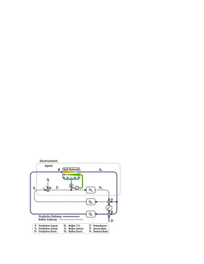
The learning platform for Sign and Relevance (SaR) is depicted in Figure 1. The underlying concept involves a fixed feedback controller, which endeavours to maintain a desired state and generates an error signal by comparing its desired state with the actual state. For instance, this may involve aiming for a target location. The error signal is then used to facilitate learning in another adaptive loop (Verschure and Coolen, 1991a; Porr and Wörgötter, 2003). Essentially, this adaptive loop learns the forward model of the fixed control loop, which is referred to as the “reflex” mechanism. The transfer functions and correspond to the environment for reflex and predictive mechanisms, respectively. Similarly, corresponds to the transfer function of the reflex mechanism itself. These functions translate actions into sensory consequences ( and ), and vice versa (). In the context of control systems, these functions are measured using system identification techniques, for example measured input-output data (Chen and Haddad, 2017). In the context of model-based learning, however, the network readily generates the forward model of the environment. The system does not rely on any previous knowledge of the environment and thus these functions are not computed in this work. The reflex mechanism, the learning pathway, and the flow of signals are described in detail below.
2.1 The reflex loop
Reflexes are among the most innate drivers of an organism’s behaviour. They are triggered involuntary actions that are carried out without prior knowledge of the stimuli. Typically, a reflex serves to ensure the survival and success of the agent. In this work, the agent is a navigational robot that aims to follow a path. When encountering a bend in the path, this innate reflex mechanism provides the organism with an immediate reaction that is designed to recover from the disturbance. Therefore, a reflex can be thought of as a fixed closed-loop controller that opposes collective disturbances while maintaining its desired state.
The desired state, denoted as located at node \small{2}⃝, represents the state that the agent aims to achieve in order to maximise its reward. In error-based learning, which is the method employed in this study, corresponds to the state where the punishment is minimised instead, meaning that the error is zero. Typically, the desired state is specified as a goal or objective for the agent to pursue. When the agent reaches this state, it achieves inner equilibrium and stability despite any external disturbances, and therefore no further action is required from the agent.
When a disturbance propagates through the reflex environment (refer to Figure 1), it triggers a change in the agent’s state. This actual state of the agent, denoted as , is continuously compared to the desired state, and any discrepancies between the two are detected by the agent’s sensors. Such discrepancies generate an error signal known as the Control Error ():
| (1) |
In technical terms, the desired state is the state in which the error signal is zero. However, if the error signal is non-zero, the reflex mechanism will take an action designed to correct for the disturbance and return the agent to equilibrium at node \small{1}⃝. This summarises the reflex pathway. Although this loop is designed to combat disturbances, it is incapable of avoiding them altogether. To maintain the desired state at all times, the reflex loop is enclosed within an outer predictive loop whose task is to mitigate the effects of the disturbance before it reaches the reflex loop.
2.2 The predictive loop
In contrast to the reflex, the Sign and Relevance (SaR) network anticipates and accounts for the disturbance with prior knowledge. This is made possible by structuring the environment so that the disturbance is delayed by time-steps, allowing the learner to generate anticipatory actions. The learner’s goal is to interact with the environment and achieve the objective without invoking the reflex mechanism. In this work, the learner aims to follow the path without relying on the reflex sensors.

The disturbance is first received by the learner’s environment and translated into predictive sensory inputs p. Based on this input information, the network generates a predictive action in an attempt to restore system equilibrium at node \small{1}⃝, where the effects of , the delayed , and the reflex action are combined before travelling through to the reflex loop. If successful, counters the delayed precisely to yield zero at this summation node, and thus the reflex loop is not evoked111Note that is zero at this instance.. However, if unsuccessful, the summation yields a non-zero signal that is received by , evoking the reflex loop and resulting in a non-zero Control Error signal.
2.3 The Control Error ()
The function of Control Error is two-fold: 1) it is received by the reflex to generate the reflex action , as described above, and 2) it serves as instructive feedback for the learner. Through iterations, the non-zero signal tunes the internal parameters of the SaR network. The learning terminates when precisely and persistently counters the disturbance at node \small{3}⃝. In this case, the reflex loop is no longer evoked, remains at zero, and the learner undergoes no further changes. Thus, the SaR network will have successfully generated the forward model of the reflex, similar to the model-based learning paradigms presented in the work by Porr and Wörgötter (2002, 2006, 2003).
2.4 The SaR learner
The learner generates the forward model of the reflex by mapping its predictive actions onto a set of sensory consequences, which is realised by the agent - the Control Error signal. The unique property of the SaR paradigm is that the instructive feedback of is facilitated through two distinct pathways: 1) the top-down pass of the sign of (green traces), and 2) global intervention of the rectified (blue traces); see Figure 1.
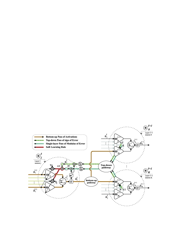
Figure 2 illustrates these pathways in detail. The symbols used for each neuron type are introduced in Panel 2A, which includes neurons in the input, hidden, and output layers. The input neurons receive the predictive signal to be injected into the network. The hidden layers contain the Control Error, their internal error (sign and modulus of), and their activation. Finally, the output neurons contain the Control Error and the final predictive motor action of the network.
The SaR learner employs a conventional feed-forward neural network with fully-connected layers. Panel 2B shows the forward pass of signals in the network, from the predictive inputs to activations in hidden layers and predictive outputs in the output layer.
Panel 2C shows the top-down pass of the sign of the error . The green traces mark the entry of the error from the reflex loop onto the output neurons. The sign of the error is passed from the final layer to the deeper layers. Within each layer, the sign of the resulting value is passed to the deeper layers. This results in an error of within each neuron, which primes their connections to be strengthened () or weakened (). This is analogous to LTP and LTD in the context of neurophysiology.
Figure 2D illustrates the single-layer traversal of the modulus of . The blue traces represent the entry of this signal from the closed-loop platform into each layer. This value activates each neuron and is transmitted only to its adjacent deeper neurons. The absolute value of the resulting sum determines the extent to which the previously primed connections are strengthened or weakened. This mechanism is similar to the effect of neuromodulators on plasticity, particularly serotonin.
3 Mathematical derivation of Sign and Relevance (SaR) learning
In this section, we derive the learning rule for the Sign and Relevance (SaR) paradigm. First, the bottom-up pass of predictive inputs is derived, following the conventional flow of signals in fully-connected feed-forward neural networks. Next, a mathematical expression of the learning goal in its general sense is presented, where a differentiable function is optimised through adjustments of weights. Subsequently, this learning goal is unravelled with respect to the closed-loop platform and the inner workings of the neural network. This leads to the derivation of the learning rule for a conventional Gradient Descent Method (GDM), which in turn provides the formulation of the SaR update rule.
3.1 Bottom-up pass of activations
Figure 3 illustrates the inner components of neurons and their connections. The bottom-up pass of activations, from the neuron in the layer, , to all neurons in the adjacent deeper layer, , is highlighted by yellow solid lines. The figure shows the network’s parameters in scalar mode, while for mathematical derivation, a matrix representation of parameters is adopted. Equations 2 and 3 summarise the forward pass from the input layer, through hidden layers, and to the output layer:
| Input layer | (2) |
| Hidden layers | (3) |
The notation p represents the matrix of predictive inputs to the network. Meanwhile, , , and denote the activation, sum-output, and weight matrices within the layer, respectively. Depending on the specific application, the predictive action may take the form of a linear function of output activations:
| (4) |
3.2 The learning goal
The primary objective of the learning process is to actively and consistently maintain the Control Error at zero, which is accomplished by adjusting the weight matrices. From a mathematical perspective, this learning goal is most effectively formulated as an optimisation task, in which the quadratic expression of the Control Error is minimised with respect to the weights.
| (5) |
To put it simply, our goal is to find weight matrices for all layers of the network such that the resulting action minimises , which is equivalent to driving towards zero. When framed as an optimisation task, a commonly used technique is the Gradient Descent Method (GDM), which involves adjusting an arbitrary weight in proportion to the sensitivity of with respect to the sum-output of the neuron associated with that weight.
| (6) |
Referring to Equation 3, the latter gradient yields the matrix of activation inputs to the neuron, denoted as . On the other hand, the former gradient establishes a relationship between the closed-loop signal () and an internal parameter of the network (). The predictive action (Daryanavard and Porr, 2020) serves as the link between the closed-loop platform and the neural network. Through the application of the chain rule, the closed-loop signals are effectively separated from the internal parameters of the network.
| (7) |
3.3 Dynamics of the closed-loop platform
Our objective is to derive an expression that establishes the relationship between the Control Error () and the predictive output . By substituting for in Equation 1, we obtain:
| (8) |
Hence, we arrive at:
| (9) |
where denotes the reflex loop gain and is determined experimentally. This partial gradient is known as the closed-loop gradient and is denoted by .
3.4 Inner dynamics of the neural network
We aim to derive an expression that relates the predictive output to the matrix of sum-outputs in an arbitrary layer. To this end, we can rewrite Equation 3 as follows:
| (10) |
Taking the derivative of with respect to yields:
| (11) |
The partial gradient resulting from this differentiation is referred to as the internal error, and is denoted by the matrix . It is important to note the recursive nature of this operation, where the calculation of the partial gradient in the layer depends on its calculation in the layer. Therefore, starting from the final layer, we define the function as the one that generates the predictive output given the activation matrix of the output layer:
| (12) |
Differentiation with respect to the sum-output matrix in the final layer yields:
| (13) |
The computation of the internal error in the final layer triggers the backwards top-down pass, which, in turn, yields the internal errors for all layers. The learning rule for GDM can be expressed as follows:
| (14) |
where is a scalar learning rate. The learning rule for SaR is derived in the following section.
3.5 The Sign and Relevance (SaR) learning rule
In this work, we use only the sign of the internal error for the top-down pass into deeper layers, as shown by the green dashed arrows in Figure 3. The result is a matrix of signs222This matrix only contains values of or ., represented as for each layer, and calculated as follows:
| (15) | |||||
| (16) |
This sign matrix is used to prime the weights for updating. A sign of primes the corresponding weight to increase, while causes the associated weight to decrease. A sign of leaves the weight unchanged. It is worth noting that the derivative of the sigmoid function is strictly positive and, therefore, does not influence the resulting sign matrix in Equation 16. This propagation spans the entire network, with only the resulting sign transmitted through the layers.
Once the neurons are primed, the magnitude of their excitation or depression is obtained from a single-layer pass of Control Error (). This is illustrated by the blue dashed arrows in Figure 3 and is formulated as follows:
| (17) |
where is the matrix of relevance signal in the layer. Unlike the internal error, the relevance signal is not passed from, or to, deeper layers; the control error interrupts this propagation. This means that does not depend on . Therefore, this signal can be generated simultaneously across all layers globally. For the final layer, it is computed as:
| (18) |
With this, the learning rule for the SaR network is defined as:
| (19) |
Where is the learning rate. The convergence of this algorithm depends on the product of the relevance signal and the activation of the neuron, which is inherently stable from a mathematical viewpoint. However, the experimental stability and convergence of the learning depend on various factors such as the network’s topology, weight initialisation, experimental set-up, amplitude of inputs, nature of the error signal, and more. Therefore, the algorithm’s convergence is best examined by observing weight changes, which are presented in the results section.
A mathematical comparison between the two learning paradigms reveals that they differ only in the calculation of the internal error. The internal error of the neuron is formed by the product of the sign and the relevance signal, analogous to that of the GDM. In both algorithms, the sign of the internal error is derived from the full propagation of the control error. The distinction lies in the calculation of the magnitude of the internal error. In the case of GDM, the magnitude is derived from a full propagation, which renders the algorithm susceptible to the vanishing or exploding gradient problem. In contrast, for SaR, the magnitude is derived from a single-layer propagation of the control error, making the algorithm immune to the aforementioned problem.
From a computational standpoint, the SaR algorithm enables full parallelisation since the calculation of the internal error in each layer does not rely on its computation in the deeper layer. Additionally, the sign signal can be calculated using integer operations, which require less memory than float or double types.
4 Implementation of SaR learning on a navigational robot
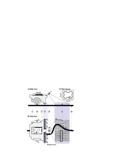
The learning algorithm presented in this study is implemented on a path-following robot, referred to as the organism, with the objective of navigating a canvas while maintaining a symmetrical position on a path printed on the canvas, also known as the environment. Refer to Figure 4C for an illustration.
4.1 The robotic platform
Schematic drawings of the robot are depicted in Figure 4A and B (not to scale). The robot’s chassis houses a battery and contains the wiring for its components. The robot is comprised of two wheels, an array of light sensors, and a camera that provides a vision of the path ahead in the form of a matrix. The SaR algorithm is hosted on a Raspberry Pi 3B+ (RPi) with a remote connection, which serves as the processing center. In the following subsections, both reflex and predictive sensory inputs, as well as the motor command, are described, and the components of the robot are discussed in detail.
4.2 Reflex sensory inputs
The light array comprises of 6 Light Dependent Resistors (LDRs) symmetrically positioned underneath the chassis in close proximity to the canvas, as shown in Figure 4A, labelled on the left and on the right333The star sign denotes the symmetrical positioning of a sensor with respect to its unmarked counterpart. side of the robot, as illustrated in Figure 4B. Each sensor detects the reflected light from a small portion of the canvas directly underneath it, referred to as the Field of View (FoV) of the sensor, as indicated by a dotted circle around sensor in Figure 4B. During navigation, these sensors convert the changes in the intensity of the reflected light into voltage fluctuations. As the FoV of a sensor transitions from capturing the black path entirely to capturing the white background, it generates a voltage potential within the range of . The Grey Value (G), denoted as depending on the sensor, is determined by linearly mapping the voltage potentials of each sensor to the range , which represents the Grey-Scale Value (GSV) of its corresponding FoV. The Grey Value of a sensor is proportional to the presence of a black path in its FoV, which provides an indication of the sensor’s vertical alignment with respect to the path and serves as an indicator for the robot’s relative positioning. For instance, in Figure 4B, sensor is vertically aligned with the path, indicating a slight overall deviation of the robot to the left, whereas the alignment of sensor would indicate a significant overall deviation to the right.
In technical terms, the robot’s deviation from the path is quantified by taking a weighted sum of the differences in the Grey Values of sensor pairs. Therefore, the experimental value of the Control Error (), which was previously defined in Equation 1, can be computed as follows:
| (20) |
Here, is a weighting factor that increases linearly with to reflect the degree of deviation. This means that the farther the active sensor is from the centerline, the greater the spike in , indicating a greater deviation. It is worth noting that, by design, there is no ground sensor at the center of the robot to detect the path when it is directly underneath the robot. The learning algorithm does not rely on explicit feedback when the robot successfully aligns with the path. The sole driver of the learning process is the error signal generated when the robot deviates from the path. Note that this error signal contains information about the direction of the solution, as its sign indicates whether the robot has veered to the left or the right of the track. This is similar to the approach presented in Porr and Wörgötter (2007b), where the error signal was utilised for training a single neuron, rather than a deep network.
4.3 Predictive sensory inputs
The camera provides information about the path in the near distance, which enables the robot to anticipate changes in the path and steer accordingly. The camera captures an image with dimensions of pixels, which is segmented into regions as shown in Figure 4B. Each square region is assigned the average GSVs of the pixels it contains, generating the sensory input from the camera in the form of an matrix . Similar to the light array sensors, the anticipated deviation in the near distance can be inferred from the difference of symmetrical entries in this matrix:
| (21) | |||
| where and |
Here, the values represent the camera signals that form an matrix. A non-zero value indicates an upcoming turn, where the value of indicates the sharpness of the turn, the value of indicates the distance of the turn from the current position, and the sign of indicates a right or left turn. Each difference signal is delayed using a Filter Array (FA) of 5 Finite Impulse Response (FIR) filters, denoted as , to achieve an optimal correlation with the Control Error signal for learning (Daryanavard and Porr, 2020):
| (22) | ||||
| where |
This leads to a sequence of 240 predictor signals which are fed into the Sign and Relevance (SaR) network to predict and generate anticipatory actions.
4.4 The Motor Command (MC)
The robot’s navigation is facilitated by adjusting the speed of its right and left wheels, and , which would otherwise move forward at a fixed speed of . A Motor Command (MC) is sent to the wheels to modify their velocities as follows:
| (23) |
The MC is generated through the joint operation of both the reflex and predictive mechanisms of the robot. As discussed in above the MC is the sum of reflex and predictive actions:
| (24) |
where is proportional to and is a weighted sum of the activations in the output layer, as indicated by Equation 12.
| (25) |
The weighting matrix allows for sharp, moderate, or slow steering of the robot, depending on the active neuron and its weight factor.
At the initial stages of a trial, is the main contributor to the Motor Command. As learning progresses, delivers a more adequate contribution. Upon successful learning, where the SaR network has generated the forward model of the reflex, is kept at zero at all times, and alone controls the Motor Command.
4.5 The architecture of the Sign and Relevance (SaR) network
This application uses a fully-connected feed-forward neural network with multiple layers. The network is initialised with random weights, but it does not use any bias terms (see Eq 2 and Eq 3). This is because the network is designed to receive predictive inputs and generate motor commands, both of which are DC-free difference signals. Additionally, the control error used to train the network is also DC-free by definition. As shown in Equation 22, the camera captures 240 inputs, and thus, the input layer of the network is initialised with 240 neurons. The network has an encoder topology, with 10 hidden layers that linearly decrease in the number of neurons: . The output layer consists of three neurons, and their weighted sum of activations, using , produces the predictive action, as shown in Equation 25.
5 Results
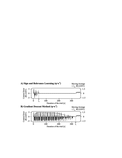
Figure 5 shows a set of trials with a learning rate of . Panels A and B display the signal of the Control Error () (solid traces) and its absolute moving average over 25 seconds, defined as (dashed traces), for the two learning modalities mentioned above. Success condition is defined as a state where falls below a value of (left-hand-side axes), which is evaluated 12 seconds after the trial has commenced, allowing the signal to accumulate.
In panel B, during a trial with GDM, the error signal is persistent for approximately 200 seconds before gradually converging and reaching the success state at time . This trial sets a benchmark for evaluating the SaR paradigm. Panel A shows the results for a trial with SaR learning, where the top-down pass of the sign of the error, and the magnitude of the error propagated one layer deep, join to drive the weight changes. It can be observed that the learning is significantly improved, as the error signal immediately begins to converge and successful learning is achieved at time .
Figure 6 shows another set of trials with a faster learning rate of . During a trial with GDM in panel B, the error signal spikes over a period of 25 seconds before fully converging at . Panel A shows that one-shot learning is accomplished during a single trial using SaR. The error signal spikes once at , and the success state is attained at . It is evident that in this trial, the moving average stays below the success threshold. Therefore, the total integral of the error provides a more reliable comparative factor, which will be depicted in Figure 11.


Figure 7 provides additional information about another one-shot learning trial with SaR. Panels A, B, and C display the Control Error signal, the activity of six selected predictive signals (marked with a rectangle in Figure 4B), and the predictive action , respectively. At time , the robot encounters the line. Prior to this moment, some predictive signals exhibit activity, but the network does not produce any steering signal ()444This is due to the robot’s initial symmetrical position on the path.. When the line is encountered, the Control Error experiences a spike that triggers a reflex reaction, returning the robot to the path and training the neural network to generate appropriate steering signals. Consequently, the error signal returns to zero at . Panel C shows a gradual increase in the network output from to , indicating the learning driven by the non-zero error signal during this interval. Once the learning is complete, the predictive signals provide the network with clues about the upcoming path, enabling it to generate appropriate predictive action. Consequently, the error signal remains at zero for the rest of the trial.
Naturally, the concept of one-shot learning in the context of deep learning raises the issue of weight stability. In this study, the Euclidean distance between weights in each layer is utilised as an indicator of weight convergence stability. This distance is calculated as the multidimensional distance between the weight matrix at time and its initialisation matrix at time :
| (26) | |||
This parameter is calculated within individual layers of the network where is constant.
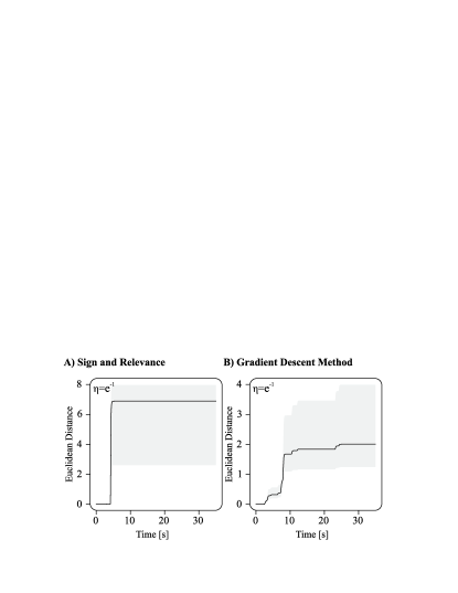
Figure 8 depicts the Euclidean distance of weights across the two trials previously illustrated in Figure 5. Panel B reveals that in a GDM trial, the final Euclidean distances of weights in deeper layers fall within a range of to (the gray area). However, changes in the first layer, which perceives the sensory consequences of motor actions, bear greater importance (Porr and Miller, 2020). Therefore, the first layer’s Euclidean distance is presented separately as the black trace, with a final distance of approximately for this trial. In Panel A, we observe this outcome for a SaR trial where the Euclidean distance is moderately greater than that of the GDM, with final distances of to for deeper layers and approximately for the first layer. Although the Euclidean distance has almost doubled, it has done so while improving the speed and performance of the SaR learner.


As mentioned previously, the first hidden layer holds greater significance as it is where the organism learns to assign importance to the sensory inputs it receives from the environment. In Figure 9, the final weight distributions in the first hidden layer for the trials previously discussed in Figures 5 and 8 are displayed. This layer comprises 240 predictive input signals and 13 neurons, resulting in a weight matrix of size by . The values in this matrix are normalised within the range of and are represented by a grey scale, with white corresponding to and black to . This creates an image of the weight distribution.
Common observations among the two learning paradigms are that 1) the eight rows of predictors (as shown in Figure 4) are appropriately classified into recognisable blocks. 2) Each block contains a gradient where the outermost columns of predictors (as seen in Figure 4) are assigned a higher value, resulting in sharper steering. 3) This gradient is more pronounced for rows of predictors closer to the robot, particularly the rightmost blocks. However, a comparison of the trials reveals a more confident and well-defined gradient for SaR learning in panel A, as opposed to the GDM in panel B.
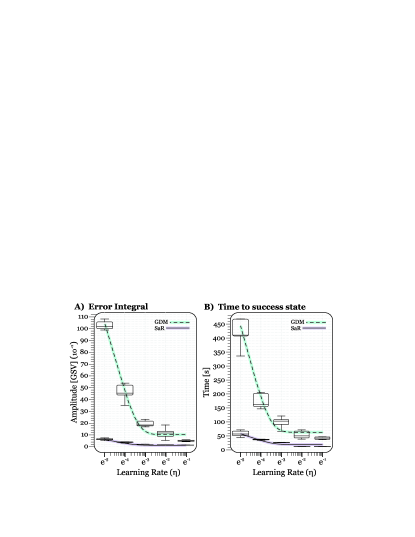
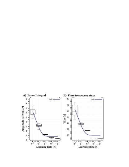
The trials depicted in Figure 5 and Figure 6 were carried out with learning rates of , with each case repeated 10 times to demonstrate the reproducibility of the results. Figures 10 A and B display the total error integral and the time taken to reach the success condition for trials conducted with SaR and GDM. It can be concluded that SaR consistently provides faster learning with smaller error accumulation, regardless of the learning rate. The comparison between the two algorithms in Figure 5 and 6 is justified by the observation that both algorithms perform best with higher learning rates and their performance declines with smaller learning rates. Therefore, Figure 6 compares the two algorithms at their best performance, while Figure 5 compares them at their worst. Furthermore, in Figures 10, it can be observed that at lower learning rates, the advantage of SaR is more pronounced. The data set for each paradigm were fitted with an exponential function of the form , which are shown superimposed on the data points. 555The coefficients a, b, and c, for error integrals are found to be: , and , and for success time: , and . Both algorithms exhibit an exponential decline with decreasing learning rates, but this decline is more rapid for GDM than for SaR. For a closer inspection, Figure 11 shows a magnified plot of the SaR data.
For a more equitable comparison between SaR and GDM, we conducted additional simulation experiments using higher learning rates to identify the optimal settings for each of these paradigms. Both paradigms failed to converge under the specified success criteria when using a learning rate of . For completeness, we considered learning rates in the set , and repeating the experiments times. The results of these experiments are presented in Figure 12. In Panel A, the results are shown for a deep neural network with an encoder topology. GDM performs best at a learning rate of , reaching an average of steps before convergence, while SaR performs optimally at , requiring an average of steps for convergence. Panel B illustrates a similar outcome for a network with a square topology. Here, both paradigms achieve their best performance at a learning rate of . GDM converges in an average of steps, while SaR achieves success in an average of steps.
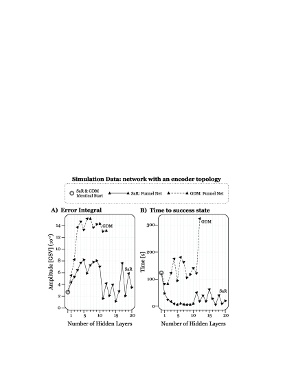
Figure 13 illustrates the effect of the number of layers in a network with a typical triangle-shaped encoder topology. The solid line represents SaR and the dashed line represents GDM. The number of hidden layers increases from 0 to 20, with the number of neurons increasing linearly for each added layer: . Zero hidden layers indicate that the network is initialised with one input layer and one output layer, where inputs are directly fed into the output neurons. Mathematically speaking, there is no difference between the two algorithms when no hidden layers are present. This has been experimentally demonstrated, as both algorithms produce identical results. Interestingly, the SaR algorithm is less affected by variations in the number of layers, as expected from its single-layer propagation. On the other hand, the GDM algorithm shows a decrease in performance as the number of layers increases. It is worth noting that there are no data points for GDM with more than 12 hidden layers since the success condition was not met (convergence was not achieved), which is due to the vanishing gradient problem. It is evident that the SaR network continues to perform well with as many as 20 hidden layers without significant changes in the results shown.
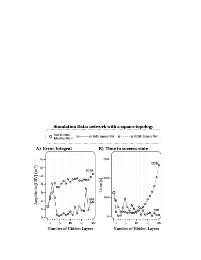
In a triangle-shaped encoder network, the total number of neurons increases drastically with each added layer. To make a more accurate comparison between the two paradigms, another set of simulations was conducted using a square-shaped network where the number of neurons was fixed at 10 per layer for each added layer: . Figure 14 illustrates the results of these experiments. As the number of hidden layers increases, both algorithms show some improvement. However, as the number of layers continues to grow, the SaR algorithm is less affected by the depth of the network, whereas the GDM algorithm progressively declines in performance. For GDM, the time taken to achieve success grows exponentially with an increasing number of hidden layers, and the error integral shows a linear growth. This indicates that GDM suffers from the vanishing gradient problem in deep networks, unlike its SaR counterpart.
A comparison of the two topologies reveals that both algorithms perform better with a square-shaped network where the number of neurons is the same across all layers. This is expected because any increase in the number of neurons in triangle-shaped encoder networks directly affects the weighted sums of inputs and the internal errors in the forward and backward passes, respectively. As a result, the propagation is more susceptible to unstable changes, which can negatively impact performance.
6 Discussion
In this paper, we introduce a learning algorithm that decomposes the error signal into a global and sign component. The sign component is passed in a top-down manner through the network, while its rectified value is transmitted globally to all layers. Unlike classical back-propagation, this approach is significantly faster in a closed-loop learning task and more closely aligns with neurophysiology by incorporating both neuromodulators and calcium-driven Long-Term Depression (LTD) or Long-Term Potentiation (LTP). We demonstrate successful learning in a simple line-following task, and this approach can be applied to any task where a fixed closed-loop “reflex” controller generates an error signal. Additionally, this approach potentially enables multi-modal processing, as any input can be used to learn a forward model of the reflex.
Deep learning has gained widespread popularity over the last decade. As it utilises neural networks, it is a promising candidate to explain how the brain itself learns (Marblestone et al., 2016). For instance, Lillicrap et al. (2016) has mapped deep learning onto the cortex, but has not considered global neuromodulation such as serotonin or dopamine.
On the other hand, traditional biologically realistic reinforcement learning models (Schultz and Suri, 2001; Wörgötter and Porr, 2005; Prescott et al., 2006) employ the reward prediction error, which bears a strong resemblance to the dopaminergic signal in the striatum (Schultz et al., 1997). These models are certainly closer to biology, but they suffer from the problem that any global error signal poses for deep structures. That is, the different layers change similarly, and hence, deep structures do not add much to their performance.
However, it remains unclear whether reward-related neuromodulators convey error signals, as has been the dominant paradigm over the last two decades (Schultz et al., 1997). Serotonin, for example, appears to encode both reward and punishment expectation (Li et al., 2016; Crockett et al., 2009; Cohen et al., 2015). We have mathematically subsumed this into a “modulus”, but in the neurophysiological context, it may be more appropriate to refer to it as a “relevance signal” because it switches on plasticity, as suggested by Porr and Wörgötter (2007a). Similarly, the negative response of dopamine neurons to a negative reward expectation has been deemed unreliable by Schultz (2004) themselves, due to its low baseline firing rate of approximately 1 Hz, which leads to a very low signal-to-noise ratio. A different interpretation for both the serotonin and dopamine signals is that of a relevance signal (Porr and Wörgötter, 2007a), ramping up or enabling plasticity (Lovinger, 2010; Iigaya et al., 2018), while local plasticity learning rules determine if synaptic weights undergo Long-Term Potentiation (LTP) or Long-Term Depression (LTD) (Castellani et al., 2001; Inglebert et al., 2020).
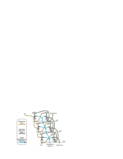
Having established global neuromodulation and local plasticity, we can now discuss how such processing can be implemented in a biologically realistic fashion. Figure 15 depicts the suggested circuit, inspired by the work of Larkum (2013); Rolls (2016), and with added neuromodulatory innervation (Lovinger, 2010; Iigaya et al., 2018). This circuit consists of two distinct pathways. The bottom-up pathway conveys, for example, sensor signals to deeper brain structures or directly to motor outputs. A single bottom-up path is depicted from the input, labelled “In”, to the output, labelled “Out”, via three synapses connecting the three neurons in layer zero (L0) to layer two (L2). Having described the bottom-up path, we can now turn to the top-down path, which controls the sign of learning (as defined in Eq. 16) and ultimately determines which neurons undergo Long-Term Potentiation (LTP) or Long-Term Depression (LTD). The bottom-up pathway transmits the sign of the error signal from layer two back to layer zero. This pathway also consists of three synapses. Additionally, there is global neuromodulation that controls the plasticity of all neurons (as defined in Eq. 17). To link this to neurophysiology, we use the well-established mechanism for driving standard neuronal plasticity, which is the concentration of postsynaptic calcium. To justify our binary switch between Long-Term Potentiation (LTP) and Long-Term Depression (LTD) (as defined in Eq. 16), we follow the reasoning of Inglebert et al. (2020): only a strong calcium influx caused by both somatic burst spiking and dendritic calcium spikes will result in Long-Term Potentiation (LTP), while less in to Long-Term Depression (LTD) (Tamosiunaite et al., 2007). Conventional backpropagation dictates that the plasticity changes for each synapse depend on the precise magnitude of the synaptic changes of deeper neurons, necessitating symmetrical weights in the both pathways. However, the network-wide binary propagation of the internal error (Equation 16) relaxes this requirement, as neurons only need to determine whether the deeper synapse underwent Long-Term Depression (LTD) or Long-Term Potentiation (LTP).
Projections from the distal parts to the dendrites alone are insufficient to induce spiking in neurons. However, if they coincide with somatic inputs, they can cause long-lasting bursting that leads to the induction of LTP due to a large influx of calcium (Larkum, 2013). Conversely, insufficient activation of dendritic trees can initiate LTD due to a smaller calcium influx from single spikes (Inglebert et al., 2020; Shouval et al., 2002). Now, let us consider the reciprocal connections between neurons, such as those observed in L1, as depicted in Figure 15. If the neuron in the top-down pathway exhibits strong spiking activity due to high synaptic weight from L2, it will also drive the neuron in the bottom-up pathway to spike, causing a calcium influx. A strong influx will trigger LTP in the bottom-up pathway, while a small influx will result in LTD. Increased synaptic weights in the bottom-up pathway will cause strong activity, which will, in turn, drive the top-down pathway and result in more calcium influx. Therefore, the sign of the weight development between reciprocal neurons in both the top-down and bottom-up pathways is mirrored because of their reciprocal connections and their ability to boost or deprive each other’s calcium concentrations. The neuromodulator controls the learning rate by regulating the amount of either Long-Term Potentiation (LTP) or Long-Term Depression (LTD). Further research is required to investigate this model in depth using more detailed biophysical modelling, which could have positive implications for models of mental illness (Rolls, 2016).
We predict that both global neuromodulation and local calcium-driven plasticity are necessary for successful behavioural adaptation in instrumental or Pavlovian learning experiments. In particular, successful learning in the cortex requires a combination of local calcium-driven plasticity and neuromodulation. Blocking the NMDA receptor disrupts calcium-driven plasticity, and we predict that cortical reward- or punishment-based learning would also be disrupted as a result. This could suggest alternative drugs that target cortical calcium/NMDA-driven plasticity rather than neuromodulators, potentially offering new treatments for depression. If the sign of learning (i.e., LTP or LTD) is determined in the cortical circuitry and propagated through its network, disrupting this kind of error propagation would still allow for learning in general via the neuromodulator, but it would no longer be directed towards a learning goal, such as finding a reward or avoiding an aversive stimulus. Instead, learning would occur without a specific goal, which would limit its usefulness.
There is no conflict of interest in this work.
We would like to thank Engineering and Physical Sciences Research Council (EPSRC) division of UK Research and Innovation (UKRI) for funding (EP/N509668/1 and EP/R513222/1) this project.
We would like to acknowledge Jarez Patel for his valuable intellectual and technical input for the making of the robotic platform.
References
- Berthoud (2004) Berthoud H (2004) Mind versus metabolism in the control of food intake and energy balance. Physiol Behav 81(5): 781–793.
- Bliss and Lomo (1973) Bliss T and Lomo T (1973) Long-lasting potentiation of synaptic transmission in the dentrate area of the anaesthetized rabbit following stimulation of the perforant path. J Physiol 232(2): 331–356.
- Bromberg-Martin et al. (2010) Bromberg-Martin ES, Matsumoto M and Hikosaka O (2010) Dopamine in motivational control: rewarding, aversive, and alerting. Neuron 68(5): 815–34. 10.1016/j.neuron.2010.11.022.
- Castellani et al. (2001) Castellani GC, Quinlan EM, Cooper LN and Shouval HZ (2001) A biophysical model of bidirectional synaptic plasticity: Dependence on AMPA and NMDA receptors. Proc. Natl. Acad. Sci. (USA) 98(22): 12772–12777.
- Chen and Haddad (2017) Chen WH and Haddad WM (2017) System Identification and Adaptive Control: Theory and Applications of the Neurofuzzy and Fuzzy Cognitive Network Models. Academic Press.
- Cohen et al. (2015) Cohen JY, Amoroso MW and Uchida N (2015) Serotonergic neurons signal reward and punishment on multiple timescales. eLife 4: e06346. 10.7554/eLife.06346. URL https://doi.org/10.7554/eLife.06346.
- Crockett et al. (2009) Crockett MJ, Clark L and Robbins TW (2009) Reconciling the role of serotonin in behavioral inhibition and aversion: acute tryptophan depletion abolishes punishment-induced inhibition in humans. J. Neurosci. 29(38): 11993–11999.
- Daryanavard and Porr (2020) Daryanavard S and Porr B (2020) Closed-loop deep learning: Generating forward models with backpropagation. Neural Computation 32(11): 2122–2144.
- Dayan and Balleine (2002) Dayan P and Balleine BW (2002) Reward, motivation, and reinforcement learning. Neuron 36(2): 285–298.
- Dela Cruz et al. (2016) Dela Cruz JAD, Coke T and Bodnar RJ (2016) Simultaneous detection of c-fos activation from mesolimbic and mesocortical dopamine reward sites following naive sugar and fat ingestion in rats. J. Vis. Exp. (114).
- Haber et al. (1995) Haber S, Kunishio K, Mizobuchi M and Lynd-Balta E (1995) The orbital and medial prefrontal circuit through the primate basal ganglia. J Neurosci 15(7 Pt 1): 4851–4867.
- Hebb (1949) Hebb DO (1949) The organization of behavior: A neurophychological study. New York: Wiley-Interscience.
- Humphries et al. (2006) Humphries MD, Stewart RD and Gurney KN (2006) A physiologically plausible model of action selection and oscillatory activity in the basal ganglia. Journal of Neuroscience 26(50): 12921–12942. 10.1523/JNEUROSCI.3486-06.2006. URL https://www.jneurosci.org/content/26/50/12921.
- Iigaya et al. (2018) Iigaya K, Fonseca MS, Murakami M, Mainen ZF and Dayan P (2018) An effect of serotonergic stimulation on learning rates for rewards apparent after long intertrial intervals. Nature Communications 9(1): 2477. 10.1038/s41467-018-04840-2. URL https://doi.org/10.1038/s41467-018-04840-2.
- Inglebert et al. (2020) Inglebert Y, Aljadeff J, Brunel N and Debanne D (2020) Synaptic plasticity rules with physiological calcium levels. Proc Natl Acad Sci U S A 117(52): 33639–33648. 10.1073/pnas.2013663117.
- Larkum (2013) Larkum M (2013) A cellular mechanism for cortical associations: an organizing principle for the cerebral cortex. Trends in neurosciences 36(3): 141–151.
- Li et al. (2016) Li Y, Zhong W, Wang D, Feng Q, Liu Z, Zhou J, Jia C, Hu F, Zeng J, Guo Q, Fu L and Luo M (2016) Serotonin neurons in the dorsal raphe nucleus encode reward signals. Nature Communications 7(1): 10503. 10.1038/ncomms10503. URL https://doi.org/10.1038/ncomms10503.
- Lillicrap et al. (2016) Lillicrap TP, Cownden D, Tweed DB and Akerman CJ (2016) Random synaptic feedback weights support error backpropagation for deep learning. Nature communications 7: 13276. 10.1038/ncomms13276.
- Linley et al. (2013) Linley SB, Hoover WB and Vertes RP (2013) Pattern of distribution of serotonergic fibers to the orbitomedial and insular cortex in the rat. Journal of chemical neuroanatomy 48-49: 29–45. 10.1016/j.jchemneu.2012.12.006. URL http://www.ncbi.nlm.nih.gov/pubmed/23337940.
- Lovinger (2010) Lovinger DM (2010) Neurotransmitter roles in synaptic modulation, plasticity and learning in the dorsal striatum. Neuropharmacology 58(7): 951–61. 10.1016/j.neuropharm.2010.01.008.
- Lu et al. (2001) Lu W, Man H, Ju W, Trimble WS, MacDonald JF and Wang YT (2001) Activation of synaptic NMDA receptors induces membrane insertion of new AMPA receptors and LTP in cultured hippocampal neurons. Neuron 29(1): 243–54. 10.1016/s0896-6273(01)00194-5.
- Luo et al. (2015) Luo M, Zhou J and Liu Z (2015) Reward processing by the dorsal raphe nucleus: 5-HT and beyond. Learn Mem 22(9): 452–60. 10.1101/lm.037317.114.
- Maffei et al. (2017) Maffei G, Herreros I, Sanchez-Fibla M, Friston KJ and Verschure PF (2017) The perceptual shaping of anticipatory actions. Proceedings of the Royal Society B: Biological Sciences 284(1869): 20171780.
- Marblestone et al. (2016) Marblestone AH, Wayne G and Körding KP (2016) Toward an integration of deep learning and neuroscience. Frontiers in computational neuroscience 10: 94.
- Markram et al. (1997) Markram H, Lübke J, Frotscher M and Sakman B (1997) Regulation of synaptic efficacy by coincidence of postsynaptic aps and epsps. Science 275: 213–215.
- Mattson et al. (2004) Mattson MP, Maudsley S and Martin B (2004) Bdnf and 5-ht: a dynamic duo in age-related neuronal plasticity and neurodegenerative disorders. Trends in Neurosciences 27(10): 589–594. https://doi.org/10.1016/j.tins.2004.08.001. URL https://www.sciencedirect.com/science/article/pii/S0166223604002589.
- O’Reilly and Frank (2006) O’Reilly RC and Frank MJ (2006) Making Working Memory Work: A Computational Model of Learning in the Prefrontal Cortex and Basal Ganglia. Neural Computation 18(2): 283–328. 10.1162/089976606775093909. URL https://doi.org/10.1162/089976606775093909.
- Porr and Miller (2020) Porr B and Miller P (2020) Forward propagation closed loop learning. Adaptive Behavior 28(3): 181–194.
- Porr and Wörgötter (2003) Porr B and Wörgötter F (2003) Isotropic Sequence Order learning. Neural Comp. 15: 831–864.
- Porr and Wörgötter (2003) Porr B and Wörgötter F (2003) Isotropic-sequence-order learning in a closed-loop behavioural system. Philosophical Transactions of the Royal Society of London A: Mathematical, Physical and Engineering Sciences 361(1811): 2225–2244.
- Porr and Wörgötter (2006) Porr B and Wörgötter F (2006) Strongly improved stability and faster convergence of temporal sequence learning by using input correlations only. Neural computation 18(6): 1380–1412.
- Porr and Wörgötter (2002) Porr B and Wörgötter P (2002) Isotropic sequence order learning using a novel linear algorithm in a closed loop behavioural system. Biosystems 67(1-3): 195–202.
- Porr and Wörgötter (2007a) Porr B and Wörgötter F (2007a) Learning with “Relevance”: Using a Third Factor to Stabilize Hebbian Learning. Neural Computation 19(10): 2694–2719. 10.1162/neco.2007.19.10.2694. URL https://doi.org/10.1162/neco.2007.19.10.2694.
- Porr and Wörgötter (2007b) Porr B and Wörgötter F (2007b) Learning with “Relevance”: Using a Third Factor to Stabilize Hebbian Learning. Neural Computation 19(10): 2694–2719. 10.1162/neco.2007.19.10.2694. URL https://doi.org/10.1162/neco.2007.19.10.2694.
- Prescott et al. (2006) Prescott TJ, González FMM, Gurney K, Humphries MD and Redgrave P (2006) A robot model of the basal ganglia: behavior and intrinsic processing. Neural networks 19(1): 31–61.
- Roberts (2011) Roberts AC (2011) The importance of serotonin for orbitofrontal function. Biol. Psychiatry 69(12): 1185–91. 10.1016/j.biopsych.2010.12.037.
- Rolls (2016) Rolls ET (2016) Reward systems in the brain and nutrition. Annual review of nutrition 36: 435–470.
- Rolls and Grabenhorst (2008) Rolls ET and Grabenhorst F (2008) The orbitofrontal cortex and beyond: From affect to decision-making. Progress in Neurobiology 86(3): 216–244. https://doi.org/10.1016/j.pneurobio.2008.09.001. URL https://www.sciencedirect.com/science/article/pii/S0301008208000981.
- Schultz (2004) Schultz W (2004) Neural coding of basic reward terms of animal learning theory, game theory, microeconomics and behavioural ecology. Curr Opin Neurobiol 14(2): 139–147.
- Schultz et al. (1997) Schultz W, Dayan P and Montague PR (1997) A neural substrate of prediction and reward. Science 275: 1593–1599.
- Schultz and Suri (2001) Schultz W and Suri RE (2001) Temporal difference model reproduces anticipatory neural activity. Neural Comp. 13(4): 841–862.
- Shouval et al. (2002) Shouval HZ, Bear MF and Cooper LN (2002) A unified model of NMDA receptor-dependent bidirectional synaptic plasticity. Proc. Natl. Acad. Sci. (USA) 99(16): 10831–10836.
- Sutton (1988) Sutton R (1988) Learning to predict by method of temporal differences. Machine Learning 3(1): 9–44.
- Takahashi et al. (2017) Takahashi YK, Batchelor HM, Liu B, Khanna A, Morales M and Schoenbaum G (2017) Dopamine neurons respond to errors in the prediction of sensory features of expected rewards. Neuron 95(6): 1395–1405.e3. https://doi.org/10.1016/j.neuron.2017.08.025. URL https://www.sciencedirect.com/science/article/pii/S0896627317307407.
- Tamosiunaite et al. (2007) Tamosiunaite M, Porr B and Wörgötter F (2007) Self-influencing synaptic plasticity: Recurrent changes of synaptic weights can lead to specific functional properties. Journal of Computational Neuroscience 23(1): 113–127. 10.1007/s10827-007-0021-2. URL https://doi.org/10.1007/s10827-007-0021-2.
- Verschure and Coolen (1991a) Verschure P and Coolen A (1991a) Adaptive fields: Distributed representations of classically conditioned associations. Network 2: 189–206.
- Verschure and Coolen (1991b) Verschure PF and Coolen AC (1991b) Adaptive fields: Distributed representations of classically conditioned associations. Network: Computation in Neural Systems 2(2): 189–206.
- von Uexküll (1926) von Uexküll BJJ (1926) Theoretical biology. London: Kegan Paul, Trubner.
- Wood et al. (2017) Wood J, Simon NW, Koerner FS, Kass RE and Moghaddam B (2017) Networks of VTA Neurons Encode Real-Time Information about Uncertain Numbers of Actions Executed to Earn a Reward. Front Behav Neurosci 11: 140. 10.3389/fnbeh.2017.00140.
- Wörgötter and Porr (2005) Wörgötter F and Porr B (2005) Temporal sequence learning, prediction and control - a review of different models and their relation to biological mechanisms. Neural Comp 17: 245–319.