Noether charges: the link between empirical significance of symmetries and non-separability

Abstract

A fundamental tenet of gauge theory is that physical quantities should be gauge-invariant. This prompts the question: can gauge symmetries have physical significance? On one hand, the Noether theorems relate conserved charges to symmetries, endowing the latter with physical significance, though this significance is sometimes taken as indirect. But for theories in spatially finite and bounded regions, the standard Noether charges are not gauge-invariant. I here argue that gauge-variance of charges is tied to the nature of the non-locality within gauge theories. I will flesh out these links by providing a chain of (local) implications: ‘local conservation laws’${\Rightarrow}$ ‘conserved regional charges’ $\Leftrightarrow$ ‘non-separability’ ${\Leftrightarrow}$ ‘direct empirical significance of symmetries’.

1 Introduction

The goal of this paper is to argue for a chain of (informal) implications for gauge theories: ‘local conservation laws’$\stackrel{{\scriptstyle*}}{{\Rightarrow}}$ ‘conserved regional charges’ $\Leftrightarrow$ ‘non-separability’ ${\Leftrightarrow}$ ‘direct empirical significance of symmetries’. To forge the necessary links, I will need two raw materials: (i) the relation between symmetries and conservation, which encompass the first three arrows, and (ii) the relation between non-separability and conserved charges, which forges the third link. The link between direct empirical significance and the non-separability will here only be referred to; it is studied in depth in Gomes (20192).

I first delineate the relevant topics in the two following subsections as a prospectus to the parts of the paper corresponding to (i) and (ii). Then section 1.3 summarizes the plan.

1.1 Noether theorems and gauge-invariant charges

The theorems proved by Emmy Noether more than a century ago have had a profound impact on both physics and mathematics. The core idea is to relate the occurrence of symmetries of the Lagrangian to conservation laws. In recent philosophy of physics, this empirical significance of symmetries—that they yield conserved charges—has been called “indirect”, in contrast to the directly empirically significant symmetries, exemplified by the subsystem-boosts of Galileo’s ship scenario Brading  Brown (2004); Greaves  Wallace (2014); Teh (2016); Friederich (2014); Gomes (20192)

However, in the case of gauge theories, the Noether relations do not guarantee gauge-invariance of the local charges. Indeed, intuition based on the Abelian case is misleading: for in this case, the local conservation law of electromagnetism yields a well-defined gauge-invariant conserved charge in an entire region of spacetime by integration (by the Gauss law).

Here I will use the covariant symplectic formalism—which does not require a foliation of spacetime into equal-time surfaces—to show that in the non-Abelian case the standard Noether charge, although conserved, is not gauge-invariant, and cannot, in general, be written solely in terms of the matter degrees of freedom. That is, beyond the lack of gauge-invariance, the generic conserved charges guaranteed by Noether’s theorems will involve more than just the standard matter degrees of freedom: they will include extra contributions from the gauge field (from the potential in the non-Abelian Yang-Mills case and from the Christoffel symbols in the gravitational case).

I find it opportune to say a few more words on this parallel with general relativity (another nonlinear theory). There, the analogous (naive) Noether charge is known as the Landau-Lifschitz pseudo-tensor; this tensor is indeed conserved, but it is coordinate-dependent and depends on the values of the Christoffel symbols in the bulk of the region. In general relativity, one can obtain coordinate-independent conserved charges that are independent of the gravitational forces, but one can do so only in very specific models of the theory (see de Haro’s contribution to this volume). Namely, when the background metric is ‘uniform’: that is, when the metric has associated Killing vector fields in the directions of uniformity, for each one of these Killing directions one obtains conserved charges written as local integrals of solely the matter part of the energy-momentum tensor (minimally coupled). The same occurs for non-Abelian Yang-Mills fields: for each gauge transformation leaving the gauge-field configuration invariant over the entire region—just as e.g. Poincaré transformations leave the Minkowski metric invariant—there corresponds a conserved charge. This analysis thereby constrains the existence of regional gauge-invariant non-Abelian charges to very specific circumstances, as it does for general relativity.

Once we have established the existence of these charges, we will have forged the links ‘local gauge symmetries’$\Rightarrow$ ‘local conservation laws’$\stackrel{{\scriptstyle*}}{{\Leftrightarrow}}$ ‘conserved regional charges’, where the asterisk signals the special conditions that allow for conserved regional charges in the sense above.

The subtle point about the gauge-invariance of charges is important in establishing the remaining links between conserved regional charges, non-separability, and Direct Empirical Significance (DES).

1.2 Non-separability and direct empirical significance

Gauge theory has often been described as a theory that exhibits excess structure; or, in John Earman’s words, “descriptive fluff” Earman (2004). But when is “fluff” merely decorative and when does it perform a function?

I have elsewhere argued—broadly in line with standard physics folklore—that the “descriptive fluff” associated to gauge theory is a sign of a particular type of non-locality, one that does not introduce any superluminal signalling. I have further argued that local gauge theories such as Yang-Mills are characterized by this non-locality, which shows up for any choice of variables.

Even in standard electromagnetism, employing gauge-invariant electric and magnetic field variables, differential constraints on the initial data prohibit an arbitrary specification of the electric field at each point. Naively, knowing the value of the electric flux on a sphere very far away can uniquely fix the total amount of charge contained in a much smaller region, at any instant, even if the matter fields are unsupported at that far away sphere. More mathematically, solving the constraint differential equations at a given point requires integration, or the inversion of differential operators, which in their turn require conditions on some surrounding boundary. This is in contrast to the initial value problem for other dynamical systems such the Klein-Gordon scalar field, which is unconstrained.

Indeed, the lesson of the Aharonov-Bohm experimental confirmation is that observables of the theory are given by non-local equivalence classes. As emphasized by Earman in Earman (2019), a certain type of non-locality of electromagnetic phenomena is the lesson of the experiment. In Earman’s words:

Thus, despite the fact that non-simple connectedness (of the electron configuration space) is essential, by definition, to the AB effect, it is not essential to some of the key issues to which it served to call attention. The philosophical literature seems incapable of absorbing this fact, as if it were under the thrall of the patently invalid inference that goes: ‘The AB effect uses non-simple connectedness; the AB effect reveals a [certain] kind of nonlocality; ergo the nonlocality derives from non-simple connectedness.’ (p.196)

Belot (1998) packs a similar message: “Until the discovery of the Aharonov-Bohm effect, we misunderstood what electromagnetism was telling us about our world” (p. 532).

Thus the question is not whether gauge theory is non-local, but how non-local it is. In trying to answer this, using holonomies as a gauge-invariant basis of vacuum electromagnetism, Myrwold argued, in Myrvold (2010), that when non-simply connected manifolds are decomposed into simply-connected pieces, there is information in the physical states of the whole that is not exhausted by the information contained in the physical states of the pieces.

Similarly—but more generally—here non-separability will be characterized as a failure of global supervenience on regions Gomes (20192). This failure occurs when the physical states of the regions fail to determine the state of the whole, and there remains a physical variety of universe states compatible with the regional physical states.

In Gomes (20192) it was shown that such a non-separability, or failure of global supervenience, is tantamount to the direct empirical significance of symmetries. That is, certain rigid gauge-symmetries, when applied to subsystems, may yield physically distinct models of the theory. These subsystem symmetries are the generators of the residual physical variety that foils global supervenience on regions (more on this below).

And although Myrvold’s argument suffices to show non-separability for electromagnetism—where holonomies have simple composition properties and form a basis for gauge-invariant functions—it does not suffice for non-Abelian theories. To analise Non-Abelian theories, we require new tools.

For to characterize how states of the universe supervene on the regional states, we must first be able to characterize the physical content of each region independently of the other. To answer these questions, my main proposal will be that, given any bounded region, one can split the degrees of freedom into ones that require extra data at the boundary for their definition from those that do not require further information. This distinction makes it easier to characterize ‘non-separability’ and also non-locality in gauge theories. In the Euclidean case, the split corresponds to a decomposition of the degrees of freedom of the gauge potential into ‘pure-gauge’ degrees of freedom and gauge-fixed, physical degrees of freedom. In the Lorentzian case, this split maps onto a Coulombic component for the electric field—which carries the boundary information—and the quasi-local radiative components of the electric field, which do not require boundary data but carry dynamical information. (this split was performed explicitly, also for non-Abelian Yang-Mills theories, in Gomes  Riello (2019); see appendix B). For simplicitly, we adopt a unified nomenclature and label both the Lorentzian radiative and the Euclidean gauge-fixed modes as radiative, and the Euclidean pure-gauge and Lorentzian Coulombic as Coulombic.

Once we have this decomposition at hand, we can investigate non-separability through a gluing/reconstruction theorem. The idea is that a manifold $M$ is divided into a patchwork of regions, mutually exlusive, but jointly exhaustive. Although in the Lorentzian case (but not in the Euclidean) the Coulombic information is essential for specifying the complete state of a single region, this data becomes superfluous once one has the (interior) radiative degrees of freedom of all the regions. In other words, in both the Lorentzian and the Euclidean signatures, knowledge of the pure radiative field content of each and every region can suffice to reconstruct the complete state of the field over the entire manifold; in this case knowledge of the regional Coulombic degrees of freedom adds no relevant information. In this sense, from the global perspective, these Coulombic degrees of freedom are indeed ‘descriptive fluff’. From the perspective of an individual region however, we must retain these degrees of freedom for a full description.

But there is a caveat to the claims of reconstruction above: the reconstruction goes through without the aid of Coulombic data only for simply-connected, compact manifolds, and if one of the two conditions is met: (a) the regional field configurations have no isometries, or (b) no charged matter is present anywhere.

When the fields have regional isometries and charged matter is present (i.e. when neither (a) nor (b) obtains), or when the underlying manifold is not simply-connected, the radiative information of the two (simply-connected) regions does not suffice to determine the entire global state. That is: there is gauge-invariant information in the global state which is not contained in the union of the regional, strictly interior, information. Assuming the underlying global manifold is simply-connected, the remaining global, gauge-invariant information—that which is not determined by the strictly interior content of the subsystems—is strictly relational and can be mapped bijectively to (subgroups of) the charge group of the theory (e.g. U(1), or SU(N), i.e. a global Lie group).

This occurrence of subgroups of the charge group arise therefore as a physical variety of global states corresponding to the same strictly interior (i.e. radiative) states. In Gomes  Riello (2019); Gomes (20192), such a variety was taken to characterize a direct empirical significance of symmetries (DES), for the variety can be construed as the result of an action of a (subgroup of the) charge group on a subsystem. Since this action takes one global state to a physically different global state, the empirical significance of these subsystem symmetries is labeled ‘direct’. But, most relevant for this paper, this underdetermination, or holism, occurs precisely when non-trivial gauge-invariant, conserved matter charges also exist. In this way, the indirect significance of gauge symmetry associated with the Noether theorems becomes intimately connected to the direct significance of gauge symmetry. In this way, we forge the remaining links between ‘local conservation laws’$\stackrel{{\scriptstyle*}}{{\Rightarrow}}$‘conserved regional charges’ $\Leftrightarrow$ ‘Non-separability’ ${\Leftrightarrow}$ ‘direct empirical significance of symmetries’.

In this chain, we restrict ourselves to spacetimes that are contractible and to standard gauge theories (including general relativity, cf. De Haro’s contribution in this volume). The asterisk applies to the non-Abelian case, since local conservation laws imply a regionally conserved matter charge only for special models of the theory.

1.3 Road map

The first link—that local gauge symmetries lead to local conservation laws—is the subject of section 2. This link of course lies within the purview of Noether’s theorems; I will summarize a version of these theorems and illustrate it with one Abelian and one non-Abelian theory.

Through these examples, we will see that the standard charges are only gauge-invariant for the Abelian theory; they are gauge-variant in the non-Abelian theory. Equivalently, the charge that is conserved will depend on both the matter fields and the gauge potentials. When matter and gauge-field contributions to the Lagrangian

I will then argue that a gauge-invariant regional notion of charge exists (cf. footnote 3), but it is non-trivial only in the presence of Killing fields (or regional isometries).

In section 3, I will summarize a split of regional degrees of freedom into “radiative” and “Coulombic”. The radiative degrees of freedom are regionally interior and non-local: that is, they are determinable solely from the regional content of the fields, without recourse to boundary data, but they are still non-locally defined within the region. The Coulombic degrees of freedom carry all the remaining information from outside a given region that is necessary to completely determine the state within the the region. Therefore, Coulombic degrees of freedom are ‘more non-local’ than the radiative degrees of freedom. With knowledge of all the radiative degrees of freedom of all the regions, it is possible to reconstruct the entire physical state (including Coulombic components).

In the conclusions (section 4), I put the results of the previous two sections together in my chain of implications. Local gauge symmetries lead to local conservation laws, which lead to a type of non-separability, which lead both to the gauge-invariant regional charges of 2 and to what I have elsewhere interpreted to be the ‘direct empirical significance of symmetries’ (see section 1.2 and Gomes (20192)).

In appendix A I will very briefly introduce the covariant symplectic formalism Crnkovic  Witten (1987); Lee  Wald (1990). The formalism is extremely convenient for the treatment of conservation laws and provides a clear path between Lagrangian/covariant concepts and Hamiltonian/canonical ones.

2 Abelian and non-Abelian Noether regional charges

In this section, I will give an abridged version of Noether’s theorems that is sufficent for my purposes. To do that, I require the rudimentary notions of the covariant symplectic formalism, developed in Crnkovic  Witten (1987); Lee  Wald (1990). The purpose of this section is to establish a useful, minimal version of Noether’s theorem using that formalism. It can be skipped by those familiar with Noether’s theorems.

First, for simplicity, suppose we are given the contractible $d$-dimensional spacetime manifold $M$ and the Lagrangian configuration space of fields on $M$, $\Phi:=\{\varphi^{I}\in C^{\infty}(M,W)\}$, for $W$ some vector space (to which the superscript $I$ refers). These fields are not yet required to solve any equation of motion. In cases of interest, $\Phi$ has the structure of a (infinite-dimensional) manifold, which we can use to formulate, among other things, its tangent bundle, $\mathrm{T}\Phi$. An element of $\mathrm{T}_{\varphi}\Phi$ is the tangent to a one-parameter family of configurations, $\frac{d}{d\lambda}_{|\lambda=0}\varphi^{I}(x,\lambda)$. By standard convention, a general such vector based at $\varphi$ is called $\delta\varphi$. In terms of a field-space basis, $\varphi^{I}(x)$, we can also decompose such a vector field:

$$\delta\varphi=\int{\mathrm{d}}x\,\delta\varphi^{I}(x)\frac{\delta}{\delta\varphi^{I}(x)}\equiv\int\delta\varphi^{I}\frac{\delta}{\delta\varphi^{I}},$$

which is understood as a derivation on function(als) on $\Phi$ and henceforth we omit the spacetime dependence of the integral and of the component fields.

Since we are heuristically taking $\Phi$ to be a bona-fide differentiable manifold, we can build up exterior calculus on it as well. For that, we call the field-space exterior derivative by the double-struck ${\mathbb{d}}$, and we can extend the double-struck notation to refer to more general geometric objects in $\Phi$, such as the Lie derivative and interior contraction, $\mathbb{L}_{{\delta\varphi}},{\mathbb{i}}_{{\delta\varphi}}$. These should all be taken to represent field-space, e.g. variational, operations. So, for example, $\mathbb{L}_{{\delta\varphi}}F={\mathbb{i}}_{{\delta\varphi}}{\mathbb{d}}F={\mathbb{d}}F(\delta\varphi)=\delta\varphi[F]$ for a scalar field-space functional $F:\Phi\rightarrow\mathbb{R}$ (in some differentiability class, which we need not discuss).

2.1 Gauge transformations

Now we move on to gauge theory as it is usually formulated. We are given a Lie group $G$ (which we will explicitly set either to $U(1)$ or ${\mathrm{SU}}(N)$) and its Lie-algebra $\mathfrak{g}$. We have an extension of $G$ to the group of gauge-transformations, which we denote by ${\mathcal{G}}=C^{\infty}(M,G)$, whose group operation is just that of $G$ pointwise on $M$, i.e. for $g,g^{\prime}\in{\mathcal{G}}$, $gg^{\prime}(x)=g(x)g^{\prime}(x)$, and thus we can define the group of infinitesimal gauge transformations, ${\mathrm{Lie}({\mathcal{G}})}=C^{\infty}(M,\mathfrak{g})$, as usual.

We also assume $G$ has some action (a representation) on the vector space of local field-values of $\varphi$, i.e. $V$, and thus we again pointwise define the action $g\cdot\varphi(x)=g(x)\cdot\varphi(x)\in\Phi$. That is: we define pointwise the natural action of the group of gauge transformations on field space ${\mathcal{G}}\times\Phi\rightarrow\Phi$. Thus field-space is foliated by gauge-orbits: namely, integral curves of field-space vectors $\delta_{\xi}\varphi$ for $\xi\in C^{\infty}(M,\mathfrak{g})$, such that $\delta_{\xi}\varphi:=\frac{d}{d\lambda}_{|\lambda=0}(\exp(\lambda\xi)\cdot\varphi)\in\mathrm{T}_{\varphi}\Phi$. Again, if the Lagrangian in (A.1) is invariant in the direction of $\delta_{\xi}\varphi$, and the Euler-Lagrange equations hold, we have:

$${\mathbb{d}}\mathcal{L}(\delta_{\xi}\varphi)=E_{I}\delta_{\xi}\varphi^{I}+\nabla_{\mu}\theta^{\mu}_{I}(\varphi)(\delta_{\xi}\varphi^{I})\approx\nabla_{\mu}\theta^{\mu}_{I}(\varphi)(\delta_{\xi}\varphi^{I})\approx 0.$$ (2.1)

Following (A.5), using the coordinate-free notation of $\theta$ as a $d-1$ form, we have the regional conservation law:

$${\mathrm{d}}(\theta_{I}(\varphi)(\delta_{\xi}\varphi^{I}))\approx 0.$$

2.2 Noether and conserved currents

First, we fix our fields and the action of the gauge group. Let $\psi$ be some complex-valued scalar field, and the gauge potential be a Lie-algebra valued 1-form, $A\in\Lambda^{1}(M,\mathfrak{g})$. We will have the indices $I$ refer to the vector space $\mathfrak{g}$ (since it is also the value-space of one of the fields) and omit reference to the value space of the field $\psi$.

We define an action of $\xi\in{\mathrm{Lie}({\mathcal{G}})}$ on these variables as:

$$\delta_{\xi}A^{I} :={\mathrm{D}}\xi^{I}:={\partial}\xi^{I}+[A,\xi]^{I}$$ (2.2)

$$\delta_{\xi}\psi :=-\xi\psi$$ (2.3)

where the square brackets delimit the $\mathfrak{g}$-commutator, within which we omit Lie indices.

The Yang-Mills Lagrangian, in form language, can be written as

$$\mathcal{L}_{\text{YM}}=-\tfrac{1}{2e^{2}}(F^{I}\wedge\ast F_{I})+(i\overline{\psi}\gamma_{\mu}{\mathrm{D}}\psi)\wedge\ast{\mathrm{d}}x^{\mu}$$ (2.4)

where $F={\mathrm{d}}A+\tfrac{1}{2}[A,A]$ and $\ast$ is the Hodge dual, $\gamma^{\mu}$ are Dirac’s gamma-matrices, and ${\mathrm{D}}_{\mu}\psi={\partial}_{\mu}\psi+A_{\mu}^{I}\tau_{I}\psi$, with $\tau^{I}$ a basis for $\mathfrak{g}$, and $e$ is the Yang–Mills coupling constant. Also, $\overline{\psi}=\psi^{\dagger}\gamma^{0}$, with the understanding that $\psi$ and $\psi^{\dagger}$ have to be considered as two independent (complex) variables. The Lie algebra index $I$ is lowered with the Kronecker delta.

Now, we compute the field-space differential of the Lagrangian,

$${\mathbb{d}}\mathcal{L}_{\text{YM}}= \big{(}{\mathbb{d}}A^{I}\wedge(-e^{-2}{\mathrm{D}}\ast F_{I}-\ast J_{I})\big{)}+{\mathbb{d}}\overline{\psi}\big{(}i\gamma_{\mu}{\mathrm{D}}\psi\wedge\ast{\mathrm{d}}x^{\mu}\big{)}+\big{(}-i{\mathrm{D}}\overline{\psi}\gamma_{\mu}\wedge\ast{\mathrm{d}}x^{\mu}\big{)}{\mathbb{d}}\psi$$

$$+{\mathrm{d}}\big{(}-e^{-2}{\mathbb{d}}A^{I}\wedge\ast F_{I}+i\overline{\psi}\gamma_{\mu}{\mathbb{d}}\psi(\ast{\mathrm{d}}x^{\mu})\big{)};$$ (2.5)

from which the equations of motion are easily extracted:

$${\rm EL}^{I}_{A}=-e^{-2}{\mathrm{D}}\ast F^{I}-\ast J^{I},\qquad{\rm EL}_{\overline{\psi}}=i\gamma^{\mu}{\mathrm{D}}_{\mu}\psi,\qquad{\rm EL}_{\psi}=({\rm EL}_{\overline{\psi}})^{\dagger}\gamma^{0}.$$ (2.6)

Here the matter, i.e. the fermions $\psi$, carry a $\mathfrak{g}$-current density:

$$J^{\mu}=(\rho,J^{i})\quad\text{with}\quad J^{\mu}_{I}=\overline{\psi}\gamma^{\mu}\tau_{I}\psi=\frac{{\partial}\mathcal{L}}{{\partial}{\mathrm{D}}_{\mu}\psi}\tau_{I}\psi$$ (2.7)

This is the current whose conservation we would like to enforce, but it is not the current whose conservation falls out of Noether’s theorem.

From (2.5) (and (A.1) in the appendix), one finds that the symplectic potential is given by:

$$\theta_{\text{YM}}=-e^{-2}{\mathbb{d}}A^{I}\wedge\ast F_{I}+i\overline{\psi}\gamma_{\mu}{\mathbb{d}}\psi\ast{\mathrm{d}}x^{\mu}.$$ (2.8)

The covariant Noether current density $j_{\xi}$ is given by

$$j_{\xi}={\mathbb{i}}_{\xi^{\sharp}}\theta_{\text{YM}} =-e^{-2}{\mathrm{D}}\xi^{I}\wedge\ast F_{I}-i\overline{\psi}\gamma_{\mu}\xi\psi\ast{\mathrm{d}}x^{\mu}$$

$$=(e^{-2}{\mathrm{D}}\ast F+\ast J)_{I}\xi^{I}-{\mathrm{d}}(\ast F_{I}\xi^{I})$$

$$\approx-e^{-2}{\mathrm{d}}(\ast F_{I}\xi^{I}).$$ (2.9)

2.2.1 Local and regional, Abelian and non-Abelian conservation laws

The conservation equation ${\mathrm{d}}j_{\xi}\approx 0$ of the standard Noether current trivially follows from (2.2), but it is not a gauge-covariant conservation law. That is, it obeys: ${\partial}_{\mu}j^{\mu}_{I}=0$ but not ${\mathrm{D}}_{\mu}j^{\mu}_{I}=0$

To obtain the relation of the Noether to the matter current, $J^{\mu}_{I}$, we insert a constant $\xi^{I}(x)=\xi^{I}_{o}$, i.e. such that ${\partial}_{\mu}\xi^{I}=0$ in the first line of (2.2). Then the $\xi$-independent relation between the currents is:

$$j^{\mu}_{I}=-[A_{\nu},F^{\mu\nu}]_{I}+J^{\mu}_{I}$$ (2.10)

To arrive at a regional conservation law, we must integrate this current over a region. But here we see that, upon integration, the conservation for $j^{\mu}$ would involve not only the values of the matter fields and current in the bulk of a region, $J^{\mu}_{I}$, but also the values of the gauge potential and curvature there! This failure to decouple the conservation of fermionic matter from bosonic fields implies that we cannot easily relate the bulk integral of quantities involving matter fields with the boundary fluxes of quantities involving the forces. Thus, the relation (2.10) so far has no implications for non-locality: we must know the values of the gauge-fields everywhere, not only at a distant boundary, to infer the total amount of matter charge contained in a region.

To remedy this situation, we first obtain a current that obeys a local covariant conservation law. Of course, $J$ fills this role. Therefore, by applying the Bianchi identities to the equations of motion for $A$:

$${\mathrm{D}}_{\mu}J^{\mu}_{I}\approx 0$$ (2.11)

In the Abelian case, there is no difference between $j$ and $J$, of course, so the conservation equation is automatically covariant. But now, at least at first sight, we have lost the possibility of integrating this current to obtain a regional conservation law, and so no non-locality is apparent.

Crucially, to determine regional conservation laws, we need not the spatially constant gauge-transformations, generated by ${\partial}_{\mu}\xi^{I}=0$, but those generated by the covariantly constant ${\mathrm{D}}_{\mu}\xi^{I}=0$.

In other words, we can integrate ${\mathrm{D}}_{\mu}J^{\mu}_{I}$ against any Lie-algebra valued scalar $\xi\in C^{\infty}(M,\mathfrak{g})$ on the bounded region $R$, obtaining:

$$\int_{N}({\mathrm{D}}_{\mu}J^{\mu}_{I}\xi^{I})=-\oint_{{\partial}N}n_{\mu}\,J^{\mu}_{I}\xi^{I}+\int_{N}J^{\mu}_{I}{\mathrm{D}}_{\mu}\xi^{I}=0$$ (2.12)

But this is a bona-fide regional conservation law if $\xi^{I}$’s are such that ${\mathrm{D}}_{\mu}\xi^{I}=0$, for otherwise the integral will not generically reduce to a boundary flux.

This establishes some caveats to our usual understanding of the Noether conserved currents. Such caveats are acknowledged, but their more radical consequences are usually left unsaid: (i) ultimately, the very concept of a non-Abelian regionally conserved charge only makes sense over a uniform background (as the notion of regionally conserved energy-momentum in general relativity) and (ii) Noether charges are not invariant in the presence of boundaries to the Cauchy surface.

There is a useful parallel to be drawn here with general relativity. In general relativity, one can use the same procedure as above to find $j_{\mu}^{I}\sim\tau_{\mu\nu}$, the so-called Landau-Lifschitz pseudo-tensor (see e.g.: (Weinberg, 2005, Ch. 15.3) and (Lifshitz, 1987, Ch. 11)). But what we want is a covariant local conservation law, such as $\nabla_{\mu}T^{\mu\nu}=0$. Indeed, the energy-momentum tensor $T_{\mu\nu}$ defined in similar fashion to $J^{I}_{\mu}$ in (2.7) does satisfy this covariant local conservation law. But this only straightforwardly yields regional conservation laws if Killing vector fields are available, i.e. if there is a $\xi_{\mu}$ such that $\nabla_{(\mu}\xi_{\nu)}=0$; for then we can write a smeared equation in a bounded spacetime region $N\subset M$:

$$\int_{N}\nabla_{\mu}T^{\mu\nu}\xi_{\nu}=\oint_{{\partial}N}n_{\mu}T^{\mu\nu}\xi_{\nu}=0$$ (2.13)

where $n_{j}$ is the normal to ${\partial}N$; this yields a regional conservation law in the same way as above.

As in general relativity, in the non-Abelian Yang-Mills case generic configurations do not admit any such Killing fields, or directions of uniformity. Therefore, true regional conservation laws emerge only in the presence of matter charges and directions of uniformity in the background field.

In the chain of implications, we can formalize the asterisk as the following condition:

$$*\quad:\quad\text{over field configurations $\tilde{A}$ such that there exist $\tilde{\xi}_{I}$ with $\tilde{\mathrm{D}}\tilde{\xi}=0$}$$

(mutatis mutandis for general relativity). Thus we have secured the link ‘local conservation laws’$\stackrel{{\scriptstyle*}}{{\Rightarrow}}$ ‘conserved regional charges’, within the special models signalled by the asterisk. Although the link would also apply more generally for any field theory employing gauge potentials and matter fields that transform as in (2.2) and (2.3) (on-shell of the matter equations of motion), we will not show this here.

As mentioned in section 1.2, according to Gomes (20192) regional conservation laws are related to the type of failure of global supervenience on regions required for the existence of ‘symmetries with direct empirical significance’ (a thesis first articulated in (Gomes  Riello, 2019, Sec 4.4)). In this respect, the important point to secure this relation is not that the charges $J$ be of one specific form or another; the important point is that the conserved regional charges be associated to the Killing directions $\xi^{I}$, which are rigid. In the next section, we will examine just how this fact is related to non-separability and therefore with the direct empirical significance of symmetries.

3 Non-separability

Here we will show that for simply-connected manifolds conserved regional charges occur just in case there is a certain level of non-separability in the model. Following Myrvold, we will first investigate this matter in electromagnetism using holonomies, but adding charged scalar fields. This will make it clear, at least in electromagnetism, that there is a residual variety in reconstructing the global state from the states of the regions if and only if charges are present within the regions.

But holonomies are not sufficient to settle the question in the non-Abelian case, and thus we will resort to a gauge-fixing, in section 3.2. Once we have gauge-fixed the regional content of the field, we will use a gluing theorem to reconstruct a gauge-fixed state of the whole from that of the regions. It will be the case once more that, in the presence of regional conserved charges, one cannot reconstruct the state of the whole from the state of the parts, thus establishing the link between ‘regional conserved charges’$\Rightarrow$‘non-separability’.

Section 3.2 applies in the Euclidean signature regime. But in such a regime, matters of locality are orthogonal to matters of separability; there are in fact no matters of locality, since there is no causal propagation. But, as separability suffices to forge the link of our chain, we leave an investigation of the Lorentzian models to appendix B. There, we will locate the source of non-locality of gauge theory in the Gauss constraint. Thus to be able to discuss the state of one region independently of the state of another—a necessary independence to analyse separability—we will split the variables into a Coulombic part, that solves the Gauss constraint as in the electrostatic case, and a radiative, dynamical part. The Coulombic part is the one that relates the charge content in the bulk of the region to boundary information. However, it is only the radiative part that enters the reconstruction theorem, and the theorem suffers from the same degeneracy as in the Euclidean case.

3.1 Holonomies and non-separability

The holonomy interpretation of electromagnetism takes as its basic elements assignments of unit complex numbers to loops in spacetime. A loop is the image of a smooth embedding of the oriented circle, $\gamma:S^{1}\rightarrow\Sigma$; the image is therefore a closed, oriented, non-intersecting curve. One can form a basis of gauge-invariant quantities for the holonomies (cf. Barrett (1991) and (Healey, 2007, Ch.4.4) and references therein),

$$hol(\gamma):=\exp{(i\int_{\gamma}A)}.$$ (3.1)

3.1.1 The basic formalism

Let us look at this in more detail. By exponentiation (path-ordered in the non-Abelian case), we can assign a complex number (matrix element in the non-Abelian case) $hol(C)$ to the oriented embedding of the unit interval: $C:[0,1]\mapsto M$. This makes it easier to see how composition works: if the endpoint of $C_{1}$ coincides with the starting point of $C_{2}$, we define the composition $C_{1}\circ C_{2}$ as, again, a map from $[0,1]$ into $M$, which takes $[0,1/2]$ to traverse $C_{1}$ and $[1/2,1]$ to traverse $C_{2}$. The inverse $C^{-1}$ traces out the same curve with the opposite orientation, and therefore $C\circ C^{-1}=C(0)$. Following this composition law, it is easy to see from (3.1) that

$$hol(C_{1}\circ C_{2})=hol(C_{1})hol(C_{2}),$$ (3.2)

with the right hand side understood as complex multiplication in the Abelian case, and as composition of linear transformations, or multiplication of matrices, in the non-Abelian case.

For both Abelian and non-Abelian groups, given the above notion of composition, holonomies are conceived of as smooth homomorphisms from the space of loops into a suitable Lie group. One obtains a representation of these abstractly defined holonomies as holonomies of a connection on a principal fiber bundle with that Lie group as structure group; the collection of such holonomies carries the same amount of information as the gauge-field $A$. However, only for an Abelian theory can we cash this relation out in terms of gauge-invariant functionals. That is, while (3.1) is gauge-invariant, the non-Abelian counterpart (with a path-ordered exponential), is not.

3.1.2 Non-separability

As both Healey (Healey, 2007, Ch. 4.4) and Belot ((Belot, 2003, Sec.12) and (Belot, 1998, Sec.3)) have pointed out, even classical electromagnetism, in the holonomy interpretation, evinces a form of non-locality, which one might otherwise have thought was a hallmark of non-classical physics. But is it still the case that the state of a region supervenes on assignments of intrinsic properties to patches of the region (where the patches may be taken to be arbitrarily small)? This is essentially the question of separability of the theory (see (Belot, 1998, Sec.3), (Belot, 2003, Sec.12), (Healey, 2007, Ch.2.4), and Myrvold (2010)).

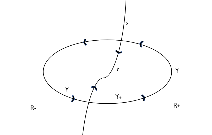
Figure 1: Two subregions, i.e. $R_{\pm}$, with the separating surface $S$. We assume no matter fields are present on $S$. A larger loop $\gamma$ crosses both regions. But, since $\gamma_{1}$ and $\gamma_{2}$ traverse $S$ along $C$ in opposite directions, $\gamma=\gamma_{1}\circ\gamma_{2}$.

We are not interested here in cases of “topological holism”, as related to the Aharonov-Bohm effect, which has been extensively studied. We are asking whether a vacuum, simply-connected universe still displays non-separability. For this topic, we can directly follow Myrvold’s definition (Myrvold, 2010, p.427) (which builds on Healey’s notion of Weak Separability (Healey, 2007, p. 46) and on Belot’s notion of Synchronic Locality (Belot, 1998, p. 540)):

$\bullet$ Patchy Separability for Simply-Connected Regions. For any simply-connected spacetime region $R$, there are arbitrarily fine open coverings $\mathcal{N}=\{R_{i}\}$ of $R$ such that the state of $R$ supervenes on an assignment of qualitative intrinsic physical properties to elements of $\mathcal{N}$.

In vacuum, it is easy to show that Patchy Separability for Simply-Connected Regions holds. In Figure 2, we see a loop $\gamma$ not contained in either $R_{+}$ or $R_{-}$. However, we can decompose it as $\gamma=\gamma_{+}\circ\gamma_{-}$, where each regional loop $\gamma_{\pm}$ does not enter the complementary region ($R_{\mp}$, respectively). Following (3.2), it is then true that, since holonomies form a basis of gauge-invariant quantities, the universal gauge-invariant content of the theory supervenes on the regional gauge-invariant content of the theory.

It is also easy to see how Patchy Separability for Simply-Connected Regions fails when charges are present within the regions but absent from the boundary $S$ (see in particular (Gomes  Riello, 2019, Sec. 4.3.2), and footnote 70 in Gomes (20192)). For, in the presence of charges, we can form gauge-invariant functions from a non-closed curve $C^{\prime}$ that crosses $S$ and e.g. one positive and one negative charge, $\psi_{\pm}(x_{\pm})$, capping off $C^{\prime}$ at $x_{\pm}\in R_{\pm}$. That is, the following quantity is a gauge-invariant function:

$$Q(C^{\prime},\psi_{\pm})=\psi_{-}(x_{-})hol(C^{\prime})\psi_{+}(x_{+})$$

for $C^{\prime}(0)=x_{-},C^{\prime}(1)=x_{+}$. It is easy to check from the transformation property $\psi\mapsto g\psi$, that $Q$ is gauge-invariant. But now, applying different rigid gauge transformations $\theta_{\pm}$, in each region will amount to choosing a different regional representation for $\psi_{\pm}$, that is, $e^{i\theta_{\pm}}\psi_{\pm}$, thus resulting in a relative shift $Q\rightarrow e^{i(\theta_{+}-\theta-)}Q$ (which, as stated above, is gauge-invariant and therefore cannot be undone by a gauge transformation). This is precisely what is known in the literature as “ ‘t Hooft’s beam-splitter” (see (’t Hooft, 1980, p.110) and and (Brading  Brown, 2004, p. 651)).

If the reader is content with the Abelian case, they may feel comfortable with skipping the next subsections.

3.2 Gauge-fixing regional and universal states

In the general non-Abelian case for bounded regions, a natural gauge-fixing suggests itself. Given a field space vector $\delta A\in T_{A}\mathcal{A}$, where $\mathcal{A}=\Lambda^{1}(M,\mathfrak{g})$ is the space of (kinematical) models for the gauge-potential, we define the Landau gauge-fixing as:

$${\mathrm{D}}^{\mu}\delta A_{\mu I}=0$$ (3.3)

In the bounded case, suppose that our patchwork of mutually exclusive, jointly exhaustive regions is given by just $R_{+},R_{-}$, such that $R_{+}\cap R_{-}={\partial}R_{\pm}$, with $s^{i}$ the normal to ${\partial}R$, and where $R_{+}\cup R_{-}=\Sigma$. We also assume $\Sigma$ to be simply-connected and without boundary, $\pi_{1}(\Sigma)=0,{\partial}\Sigma=\emptyset$. Suppose moreover that there are is no charged matter at ${\partial}R$.

In that case, the gauge-fixing (3.3) becomes:

$$\begin{cases}{\mathrm{D}}^{\mu}\delta A^{\pm}_{\mu I}=0\\ \delta A^{\pm}_{sI}=0\end{cases}$$ (3.4)

where, again, $s$ is the normal to the shared boundary of the region. We call a field-space vector that satisfies these conditions, horizontal (or radiative, in the Lorentzian case), and denote them by $h$ and $h_{\pm}$, in the global and regional cases, respectively.

It is easy to show that (3.3) and (3.4) are bona-fide perturbative, gauge-fixings, that are moreover covariant under a change of the perturbed configuration $A\rightarrow A+\delta_{\xi}A$ (and mutatis mutandi for the regional case, so that the gauge-fixing of the perturbation does not sensitively depend on the choice of representative for the perturbed configuration.

Two configurations $h_{\pm}$ are composable if and only if there exist gauge transformations, $\xi_{\pm}$, such that:

$$\delta A=(h_{+}+{\mathrm{D}}_{+}\xi_{+})\Theta_{+}+(h_{-}+{\mathrm{D}}_{-}\xi_{-})\Theta_{-},$$

where $\Theta_{\pm}$ are the characteristic functions of the regions $R_{\pm}$, is a smooth global gauge configuration. Composability therefore requires the difference of the configurations at the boundary, $(h_{+}-h_{-})_{|S}=({\mathrm{D}}_{+}\xi_{+}-{\mathrm{D}}_{-}\xi_{-})$, to be pure gauge. These matters are taken up in detail in Gomes  Riello (2019); Gomes (20192, 2020).

In general there will be many such $\xi_{\pm}$ if there is any. But to establish residual physical variety of the global state, we must also consider the variety of global physical states that will correspond to the composition, and therefore we must gauge-fix globally, with (3.3). In most cases, this global gauge-fixing will uniquely fix $\xi_{\pm}$; when it does not, there can be a residual physical variety, as we explain next.

3.3 Coulombic and radiative reconstruction theorem

To finish this section, I will present results on ‘gluing’: in reassembling the regional information of the fields into the global state of the fields, employment of the pure-gauge and horizontal (alternatively, Coulombic and radiative, cf. appendix B) split of regional degrees of freedom is remarkably instructive. (To avoid having to intersperse such parentheses along the following section, the results are framed in the unifying language of ‘Coulombic and radiatives’ modes). Again, I will only state, and not prove any of the surprising results here (see (Gomes  Riello, 2019, Sec. 4)).

3.3.1 The theorem, loosely stated

The reconstruction theorem states that in these circumstances, we can fully and uniquely reconstruct the state on the entire region, e.g. we can recover the full physical content of the fields, solely from the strictly interior degrees of freedom. Those degrees of freedom that require further boundary information—the Coulombic—are superfluos for reconstruction.

As a schematic example, in the Lorentzian case (cf appendix B), we again split the electric field and the spatial gauge potential along radiative and Coulombic components. The Coulombic component of $E$ generalizes the electrostatic electric field, and is of the form $E_{\text{Coul}}={\mathrm{D}}\Lambda$, for some (Lie-algebra-valued) scalar potential $\Lambda$ and $E_{\text{rad}}$ being divergence-free, as in (3.3): ${\mathrm{D}}^{i}E_{iI}=0$ (obeying the same Neumann boundary conditions as in (3.4)).

Thus the total regional field is $E_{\pm}=E^{\text{rad}}_{\pm}+{\mathrm{D}}\Lambda_{\pm}$, with $\Lambda_{\pm}$ satisfying the Poisson equation ${\mathrm{D}}^{2}_{\pm}\Lambda_{\pm}=\rho_{\pm}$, with $\rho_{\pm}$ related to the regional matter fields $\psi_{\pm},\overline{\psi}_{\pm}$ by (2.7), with boundary conditions on the Poisson equation given by $s^{i}{\mathrm{D}}_{i}\Lambda=s^{i}E_{i}\equiv f$. It would seem the Coulombic degrees of freedom parametrized by $\Lambda_{\pm}$ are essential for a description of the global state. Surprisingly, we can recover the global $E$ solely as a functional of those degrees of freedom which carry no dependence on the boundary conditions (i.e. the radiative ones).

The statement of the gluing theorem therefore is that, in the Euclidean case, if the perturbed potential $A^{\pm}_{\mu I}$ has either no Killing directions (i.e. no stabilizers), or no charged currents inside the regions $R_{\pm}$, then $h_{\pm}$ uniquely determines the global physical state $h$. In the Lorentzian case (for which now $R$ and $R_{\pm}$ are spatial regions), the statement is that if the phase space points $(A^{\pm}_{iI},E_{i}^{I\pm})$ have no stabilizers, the radiative components $E^{\text{rad}}_{\pm}$ and the matter charges $\psi,\overline{\psi}$, suffice to determine all the remaining regional components, $E^{\text{Coul}}_{\pm}$, and also the global ones: $E^{\text{rad}}$ and $E^{\text{Coul}}$.

For the proof, which uses the remarkable properties of the Dirichlet-to-Neuman operators, see (Gomes  Riello, 2019, Sec 5).

3.3.2 The caveats, loosely stated

But, as announced, if the necessary conditions do not obtain, there are ambiguities in the reconstruction. These occur only if the underlying fields $A^{\mu I}_{\pm}$, or, in the Lorentzian setting, $(A^{iI}_{\pm},E^{iI}_{\pm})$, admit stabilizers (or Killing vectors). Let us call such a homogeneous, or uniform potential, $\tilde{A}^{\mu I}_{\pm}$; the arising ambiguities are precisely the stabilizers of $\tilde{A}$, that we label $\chi_{\tilde{A}}$.

A gauge transformation by one such stabilizer does not affect the gauge fields (by construction, since ${\mathrm{D}}\xi=0$), but does affect the matter fields, by the transformation law (2.3). Therefore If these ambiguities exist, and there are non-trivial matter fields inside the regions, a corresponding ambiguity in the reconstruction slips in: the matter components are shifted by an element of the stabilize. Although this rotation does not affect either regional gauge-invariant state, it has a relative effect between the regions. This is precisely the same sort of regional rigid gauge shift we saw at the end of section 3.1.2, and to the ‘t Hooft beam-splitter. And these conditions are precisely the ones required for the existence of ‘conserved regional charges’. Therefore we have established the link ‘conserved regional charges’$\Rightarrow$‘non-separability’.

It is also possible at this stage to understand why in the Abelian, but not in the non-Abelian case, we always find well-defined regional gauge-invariant charges (in the presence of charged matter), thus connecting the present discussion back to section 2.2.1. Namely, for Abelian theories the existence of stabilizers $\chi$ impose no restrictions on $A$: for all $A$, the stabilizers are just the constant gauge transformations.

The same argument could be applied to general relativity: suppose there are matter fields that vanish at the intersection of two flat regions, but not in their interior. Then we could gauge-fix all the non-rigid diffeomorphisms with the metric field, but that would leave out the rigid Poincaré transformations. Then applying distinct such transformations to each region, we would have no global Poincaré transformation that would be able to efface the difference between the rigid regional transformations at the boundary. Although without the presence of matter the overall state of affairs after the tranformation would be the same as before, it would be distinct if matter was present. Those are again precisely the conditions required to obtain non-trivial regional conserved charges in general relativity.

3.3.3 The link to DES

To establish the further link to DES, we note that the ambiguity corresponds to a global—or rigid, in the nomenclature of Gomes (20192)—gauge transformation, which is necessarily a subgroup of the charge group $G$. See (Gomes, 20192, Sec. 5.2.4) and (Gomes  Riello, 2019, Sec. 4) for proofs and explicit examples. In the Abelian case of electromagnetism, there is always a conserved U(1) global transformation if charged matter fields are present in the regions.

To summarize, to obtain a left-over variety in the reconstruction of the whole from the radiative parts, we require non-trivial stabilizers and non-zero charged matter fields. Moreover, we can explicitly associate this physical variety with the action of a subgroup of $G$ on a subsystem. This action can indeed be construed as endowing ‘direct empirical significance’ to this group of global symmetries Gomes  Riello (2019); Gomes (20192). Lastly, the requirements for obtaining this variety also correspond to those for obtaining non-trivially conserved regional, gauge-invariant Noether charges.

4 Conclusions

4.1 Summary

Local conservation laws are a widely celebrated consequence of symmetries. While it is true that in certain cases one can extract conserved regional quantities from integrating the Noether densities, such charges may be problematic in other regards. For instance, the obtained regional charges may be gauge-variant. Or, when we think of fermionic charges as sourcing bosonic forces, it could be that we cannot isolate a regional conservation law for the matter charges. Both of these obstacles occur for non-Abelian Yang-Mills theory and general relativity, and both can be avoided at a single stroke: with gauge-invariant conserved regional matter charges emerging from the regional volume only if the underlying configuration admits stabilizers. This result provided the first link of the chain of implications proposed in this work.

The second link connected such regional charges with non-separability. This link followed without ancillary conditions and applies also to simply-connected regions (in the non-simply-connected case, the vacuum configurations are also non-separable by the same methods). We showed it first for the Abelian theory using holonomies and then in the non-Abelian case using gauge-fixings. Crucially, non-separability in the simply-connected case requires a gauge transformation that is an isomorphism of the gauge field but not of the matter field. If the matter field vanishes anywhere, such transformations cannot be gauge-fixed, and yet, if different such transformations are applied in each region, they will change the physical state of the union of the regions. Nonetheless, from the perspective of the region, the shifted configuration is physically indiscernible from the unshifted configuration. Thus, we obtained non-separability, and clearly, a connection with a subsystem symmetry that could be said to have empirical significance. Although Gomes (20192) fleshes out this link in more detail, here we saw a (hopefully convincing) sketch of the link, listing its main arguments.

Although the paper was focused on Yang-Mills theories, the main arguments here can be transposed without much difficulty to general relativity. In the interest of space, I have kept this parallel mostly in the background for this paper.

Moreover, a few words should be said about the generality of these links: in which sense are they merely kinematical, and in which do they depend on the specific form of the Lagrangian? The only step in which we explicitly used the Lagrangian was in obtaining the regionally conserved charges. But, for gauge-invariant theories that have $A$ and $\psi$ as variables, with the transformation properties (2.2) and (2.3), that link follows as well (on-shell of the matter equations of motion, cf. footnote 13). But I have not explored the full space of theories in which these links would hold, and therefore the implications need to be seen as “local deductions”.

4.2 An added link to locality

Local symmetries have another, less celebrated consequence: they yield constraints on the initial values, thus pointing to a mild form of non-locality in a gauge theory. As discussed in appendix B, one cannot freely specify the initial value of the electric field here without knowing what is the far away distribution of charges at that same instant.

The link to non-locality does not fit as neatly into the chain of deductions explored in this paper, although it is inextricably connected to them. So, lest we tie them together, we would be left with all those loose ends; thus the inclusion of the discussion in the appendix B (but not on the main paper) and this extended subsection here in the conclusions.

The particular non-locality of gauge theories can be examined precisely with the aid of a decomposition of the fields into Coulombic and radiative components. The radiative component corresponds to the strictly interior field content of a region; the Coulombic component depends also on boundary information.

We can track the effect of the decomposition on the Noether charges of the theory: the emerging radiative Noether charges are identical to the gauge-invariant Noether charges discussed in the first sections. The Coulombic charges can be identified with the gauge-variant charges; they correspond to the boundary gauge group: ${\mathrm{Lie}({\mathcal{G}})}_{{\partial}R}$.

In the absence of stabilizers, the radiative modes are the sole carriers of the non-redundant regional information needed to piece back together a global state. The Coulombic degrees of freedom can also be reassembled by knowledge of the regional radiative degrees of freedom and are, in that sense, superfluous. But they become superfluous only from the perspective of the whole; given any single region, they are functionally independent from the radiative modes (Gomes  Riello, 2019, Sec 5). This analysis is in accord with the proposal of Gomes (20191), which argues for the ineluctability of redundant, pure gauge degrees of freedom for the description of regions, but not for the description of the whole.

Acknowledgements

I would like to thank an anonymous reviewer, for very insightful and constructive remarks.

APPENDIX

Appendix A Symplectic formalism

A.1 The covariant symplectic formalism abridged

A given action

$$S[\varphi,\gamma]=\int_{M}\mathcal{L}(\varphi^{I},\nabla_{\mu}\varphi^{I},\nabla_{(\mu}\nabla_{\nu)}\varphi^{I},\nabla_{(\mu_{1}}\cdots\nabla_{\mu_{n})}\varphi^{I},\gamma)$$

for the Lagrangian density $\mathcal{L}$ dependent on the field $\varphi^{I}$, its derivatives up to n-th order, and some background structure $\gamma$, can be seen as a function on an appropriate n-th jet-space of $\Phi$. Using the manifold structure of $\Phi$ we can take directional derivatives of $S$ and indeed of $\mathcal{L}$.

Taking the functional derivative of $S$ along some generic $\delta\varphi^{I}$, for which we employ the standard notation for directional derivative, $\delta\varphi[S]$, we can usefully organize the result (using the jet-bundle structure) as:

$${\mathbb{d}}S(\delta\varphi)=\int\sum_{k=0}^{n}\frac{{\partial}\mathcal{L}}{{\partial}(\nabla_{(\mu_{1}}\cdots\nabla_{\mu_{k})}\varphi^{I})}\nabla_{(\mu_{1}}\cdots\nabla_{\mu_{k})}\delta\varphi^{I}=\int\left(E_{I}\delta\varphi^{I}+{\mathrm{d}}(\theta_{I}(\varphi)(\delta\varphi^{I}))\right)$$ (A.1)

Here the Euler-Lagrange density is given by:

$$E_{I}=\sum_{k=0}^{n}(-1)^{k}\nabla_{\mu_{1}}\cdots\nabla_{\mu_{k}}\mathcal{L}_{I}^{\mu_{1}\cdots\mu_{k}}$$ (A.2)

where the partial derivative functions are given by:

$$\mathcal{L}_{I}:=\frac{{\partial}\mathcal{L}}{{\partial}\varphi^{I}},\,\text{for $k=0$, and}\quad\mathcal{L}_{I}^{\mu_{1}\cdots\mu_{k}}:=\frac{{\partial}\mathcal{L}}{{\partial}(\nabla_{(\mu_{1}}\cdots\nabla_{\mu_{k})}\varphi^{I})}.$$ (A.3)

The symplectic potential density $\theta$ is a $(d-1)$ differential form in spacetime and a 1-form in field-space (it is a local linear functional on field-space vectors $\delta\varphi$). And we can express the exterior derivative of a $d-1$ form as the divergence of the corresponding vector:

$$\theta^{\mu}_{I}(\varphi)(\delta\varphi^{I}):=\sum_{k=1}^{n}\sum_{\ell=1}^{k}(-1)^{\ell+1}\left(\nabla_{\mu_{2}}\cdots\nabla_{\mu_{\ell}}\mathcal{L}_{I}^{\mu\mu_{2}\cdots\mu_{k}}\right)\left(\nabla_{\mu_{\ell+1}}\cdots\nabla_{\mu_{k}}\delta\varphi^{I}\right)$$ (A.4)

The idea now is simple. Suppose the Lagrangian in (A.1) is invariant in the direction of some particular $\widehat{\delta\varphi}$, and that the Euler Lagrange equations hold (which we signal by employing the weak equality $\approx$). If we use the coordinate-free notation of $\theta$ as a $d-1$ form, we conclude that the other term of the integrand of (A.1) weakly vanishes:

$${\mathrm{d}}(\theta_{I}(\varphi)(\widehat{\delta\varphi}{}^{I}))\approx 0,$$ (A.5)

where d is the spacetime exterior derivative. Thus by integrating over a spacetime region we can obtain the usual regional conservation laws for $\theta_{I}(\varphi)(\widehat{\delta\varphi}{}^{I})$, which is called the Noether current density for $\widehat{\delta\varphi}{}^{I}$. This is the essence of Noether’s theorems.

A.2 The covariant symplectic form and the Hamiltonian

Working now in field-space, we can introduce a symplectic structure as follows. Using the exterior derivative on the symplectic potential density, which is a field-space one-form $\theta_{I}^{\mu}$, we obtain a symplectic-form density, $\omega_{IJ}^{\mu}:=({\mathbb{d}}\theta)_{IJ}^{\mu}$, which is a $d$-1 form in spacetime and a closed 2-form in field space (since ${\mathbb{d}}{\mathbb{d}}\equiv 0$). Choosing a closed Cauchy surface $\Sigma$ (for now unbounded), we define:

$$\Omega:={\mathbb{d}}\Theta,\quad\omega_{IJ}={\mathbb{d}}(\theta)_{IJ};\quad\Theta({\delta\varphi})=\int_{\Sigma}\theta_{I}{\delta\varphi}^{I},\quad\Omega({\delta\varphi}_{1},{\delta\varphi}_{2})=\int_{\Sigma}\omega_{IJ}{\delta\varphi}_{1}^{I}{\delta\varphi}_{2}^{J}$$ (A.6)

where we have only kept the internal index $I$, which serves to remind us that we are dealing with components, also in the (suppressed) spacetime labels $\mu$ and $x$.

If the symplectic potential $\Theta$ is also gauge-invariant on-shell (which is always the case if ${\partial}\Sigma=\emptyset$, (cf. (Lee  Wald, 1990, eq. 3.22)) we can apply the Cartan Magic formula to obtain:

$$\mathbb{L}_{{\delta\varphi}}\Theta\approx 0=({\mathbb{d}}{\mathbb{i}}_{{\delta\varphi}}+{\mathbb{i}}_{{\delta\varphi}}{\mathbb{d}})\Theta$$ (A.7)

and therefore we obtain ${\mathbb{i}}_{{\delta\varphi}}\Omega\approx-{\mathbb{d}}(\Theta({\delta\varphi})),$ so that the Hamiltonian generator for the flow ${\delta\varphi}$ is simply given on-shell by $\Theta({\delta\varphi})$. Then one usually writes the Hamiltonian generator $H[\xi]$ of the gauge transformation $\xi$ as:

$$H[\xi]=\int_{\Sigma}\theta_{I}\delta_{\xi}\varphi^{I}.$$ (A.8)

Indeed, in the absence of boundaries of the Cauchy surface, we can go beyond the mere existence of a Hamiltonian generator: it is possible to show that ${\mathbb{i}}_{\widehat{\delta\varphi}}\Omega\approx 0$ for variations within the subset of field configurations which satisfy the equations of motion, in which case, the kernel $\widehat{\delta\varphi}{}$ is integrable in that subset (cf. (Lee  Wald, 1990, eq. 3.27)). More specifically, the on-shell integral manifold corresponding to the tangent vectors $\widehat{\delta\varphi}{}$ form ‘orbits’ parametrized by gauge transformations. It is then possible to constitute a finite equivalence relation along elements of the gauge-orbits and thus formally reduce the pre-symplectic to the symplectic formalism.

Moreover, note that applying a Lie derivative along $\widehat{\delta\varphi}{}$ to a gauge-invariant density $\theta$ and using ${\mathbb{i}}_{\widehat{\delta\varphi}}\Omega\approx 0$, we obtain

$$\mathbb{L}_{\widehat{\delta\varphi}{}}\theta=({\mathbb{d}}{\mathbb{i}}_{\widehat{\delta\varphi}{}}+{\mathbb{i}}_{\widehat{\delta\varphi}{}}{\mathbb{d}})\theta\approx{\mathbb{d}}({\mathbb{i}}_{\widehat{\delta\varphi}{}}\theta)\approx 0.$$ (A.9)

Therefore, for bona-fide gauge transformations—those which we can treat symplectically—the associated Hamiltonian must be on-shell field-independent. We can therefore weakly set the Hamiltonian constraints corresponding to gauge transformations to zero: $H[\xi]\approx 0$.

Appendix B Non-locality and Coulombic and radiative components

B.1 Non-locality

To fully comprehend the non-local content of the equations of motion of gauge theories, it is instructive to first examine an entirely local, extremely simple, example: that of a massless Klein-Gordon field—$\varphi\in C^{\infty}(M,\mathbb{C})$ such that ${\partial}^{\mu}{\partial}_{\mu}\varphi=0$. Given any initial values $(\varphi,n^{\mu}{\partial}_{\mu}\varphi)$ of configuration and configurational ‘velocity’ on a Cauchy surface (or on a subset thereof), we can find a corresponding solution of the Klein-Gordon equations in the domain of dependence of the region (by the Cauchy-Kowalevsky theorem). In this case, locality is a consequence of a single equation of motion, of the same order in spatial and time derivatives.

But for gauge theories, some of the differential equations of motion may contain only spatial and no time derivatives, signalling the occurrence of initial value constraints. This is the case with Yang-Mills theory. In other words, having chosen a Cauchy surface $\Sigma$, we are not free to choose any value we want for the doublet $(E^{i}_{I},\rho_{I})$ on $\Sigma$.

Let us take the simple example of electromagnetism: the Gauss law ${\partial}^{i}E_{i}=\rho$ does not allow us to choose any value for the electric field on a given point $x\in\Sigma$ independently of the distribution of charges or of the values of $E$ in other points: there are Coulombic constraints that must be first satisfied. These constraints must be satisfied even before any equation accounting for propagation in time is taken into account. Since the constraint is a spatial differential equation, resolving the constraint will require some amount of integration over a given region at a fixed time.

To see that this requirement must be satisfied before any dynamics takes place, we can take an even simpler example: the electrostatic regime, in which case $E_{i}={\partial}_{i}\phi$, where $\phi$ is the Coulombic potential. We then have to satisfy a Poisson equation, $\nabla^{2}\phi=\rho$, whose solution involves an integral of a Green’s function over the entire $\Sigma$.

But this non-locality need not be of an extreme sort! It won’t allow faster-than-light-signalling for instance. And it doesn’t necessarily involve knowledge of the charge distributions over the entire Cauchy-surface; one may exchange that completely global information for a more local one: the electric flux on the boundary of a region surrounding our chosen point $x$. That is, given a point $x\in\Sigma$, and a closed region $R$ around $x$, knowing both the charge distribution within $R$ and boundary conditions for $\phi$ on ${\partial}R$, we can establish the electrostatic field at $x$. If one knows the ‘local electric flux’ through $R$, ${\partial}_{n}\phi=E_{n}:=f$, where $n_{i}$ is the normal to $R$ within $\Sigma$, then one knows the value of the electric field in $x$.

Thus the static electric field within a region has regional locality in the sense that it is determined by the distribution of charges in the region and boundary data. It is therefore a regional quantity, but not a strictly interior one. The boundary data represents the influence of the outside on the inside of the region. This provides a specification of degrees of freedom for each region which depends only on the interior of the region, and not on any boundary information. These are what we call “radiative” degrees of freedom.

Any new split of degrees of freedoom must be checked for consistency in at least two ways. First, is the split kinematically consistent? I.e. is it obeyed by symplectic conjugacy relations? And second: how independent or redundant are the different types of degrees of freedom, when taken regionally and globally? That is, when does knowledge of one sort of information determine the state of the other? The first question will be taken up in section B.2.1, where we will prove consistency, and the second was taken in section 3.3, where we showed that although for each region the radiative degrees of freedom is entirely functionally independent of the regional $\phi$, the collection of radiative degrees of freedom associated to a patchwork of mutually exclusive, jointly exhaustive regions fully determines both the radiative and the Coulombic degrees of freedom of the whole. There is thus a subtle manner in which the Coulombic components are superfluous only when the entire collection of regional interior data is available, but not before. This is consistent with previous work, Gomes (20191), arguing that gauge degrees of freedom are superfluous only from a global perspective, but not from a parochial one.

B.2 Coulombic and radiative symplectic pairs

To establish our claims, we must further examine the source of non-locality in the dynamics of Yang-Mills theory, and that is what we will do in this section, which is based on (Gomes  Riello, 2019, Sec. 3). According to the above, at least in the standard variables, the source lies in the Gauss laws. Thus the first order of business is to segregate the Coulombic degrees of freedom from the remaining ones in the electric field. We will see that in a concrete sense the Coulombic ones are the carriers of the boundary information of the field.

B.2.1 Coulombic and radiative decomposition

We start with the standard decomposition of the electric field:

$$E_{i}^{I}=\dot{A}^{I}_{i}-{\mathrm{D}}_{i}A_{0}^{I}.$$ (B.1)

Coulombic terms are usually described as those given by the gradient of the potential, i.e. ${\mathrm{D}}_{i}A_{0}^{I}$. But $E^{I}_{i}$ can also contain Coulombic terms, i.e. terms of the form ${\mathrm{D}}_{i}\xi^{I}$, for some Lie-algebra-valued function $\xi\in C^{\infty}(\Sigma,\mathfrak{g})$. Lucky for us, there is a straightfoward way to extract the strictly Coulombic component of $E_{i}$ by employing a generalized Helmholtz decomposition. The decomposition spits out a unique covariant gradient of a Coulombic potential and another component, covariant-divergence-free, which we will call radiative, and denote as $E_{i}^{\text{rad}}$.

In other words, any $E_{i}$ in the region $R$, without any restriction on boundary values, can be uniquely decomposed into:

$$E_{i}=E_{i}^{\text{rad}}-{\mathrm{D}}_{i}\phi.$$ (B.2)

That is, both $E_{i}^{\text{rad}}$ and $\phi$ can be uniquely written as functionals of $E_{i}$ (see (Gomes  Riello, 2019, Sec. 3.2)) and, under a gauge-transformation, $E_{i}^{\text{rad}}$ transforms like the electric field and $\phi$ tranforms like $A_{0}$. For our purposes here, the precise form of these functionals is secondary; what is important to know is that the range of values $\phi$ can take are left unconstrained off-shell (i.e. before we consider how they react to charged matter), while $E_{i}^{\text{rad}}$ obeys the following equations:

$$\begin{dcases}{\mathrm{D}}^{i}E^{\text{rad}}_{i}=0&\text{in }R,\\ n^{i}E^{\text{rad}}_{i}=0&\text{at }{\partial}R.\end{dcases}$$ (B.3)

Although the radiative components are non-local within the region, they do not require any further information from outside the region.

In the next section, we will present the symplectic decoupling of the radiative and Coulombic degrees of freedom. Moreover, since the symplectic potential is intimately related to the Noether charges (see section 2), by studying the decomposition of the symplectic potential we will verify that their Coulombic and radiative parts correspond to the “problematic”, gauge-variant Noether charges, and the gauge-invariant, “non-problematic” Noether charges, respectively.

B.2.2 Coulombic and radiative symplectic potentials

The total symplectic potential, introduced in section A.1 for standard vacuum Yang-Mills for a Cauchy surface $\Sigma$ without boundaries is given by (see the first term on the rhs of (2.8)):

$$\Theta=\int_{\Sigma}E\wedge{\mathbb{d}}A$$ (B.4)

where the phase space $\mathcal{P}$ is given in the basis $(A,E)$. In the presence of boundaries, i.e. for $R\subset\Sigma$ such that ${\partial}R\neq\emptyset$, we can still translate the radiative-Coulombic decomposition of phase space variables into a decomposition of the symplectic potential into a radiative and a Coulombic component, i.e. $\Theta=\Theta^{\text{rad}}+\Theta^{\text{Coul}}$. We should note that the decomposition requires field-space one forms projecting both $\delta A,\delta E$, onto their radiative, i.e. non-Coulombic components, and onto the complementary Coulombic components.

The Coulombic symplectic potential is given by:

$$\Theta^{\text{Coul}}=\oint_{{\partial}R}f_{I}\phi^{I}.$$ (B.5)

$\Theta^{\text{Coul}}$ is a 1-form on phase-space, only acting as a one-form on one of the phase space directions: along disturbances in $A$ (as in (B.4)). So in (B.5) $\phi$ is a field-space one-form and $\phi(\delta A)$ is the ‘Coulombic extraction’ of the field-space vector $\delta A$. Since a given perturbation such as $\delta A={\mathrm{D}}\xi$ is pure-gauge, an extraction of the ‘pure Coulombic’ part of $\delta A$ is an extraction of its pure-gauge component, i.e. $\phi(\delta A)=\xi$. $f$ is the electric flux at the boundary, i.e. the normal component of the electric field there (for the complete symplectic treatment of the decomposition, see (Gomes  Riello, 2019, Sec. 3.6)). Note that the dynamical relevance of the Coulombic terms appears only at the boundary ${\partial}R$: the electric flux is conjugate to the restriction of the pure gauge (i.e. pure Coulombic) part of $A$ to the boundary.

The radiative component of the symplectic potential is given by:

$$\Theta^{\text{rad}}=\int_{R}\left(E^{\text{rad}}_{iI}{\mathbb{d}}A_{\text{rad}}^{iI}\right)$$ (B.6)

where ${\mathbb{d}}A_{\text{rad}}={\mathbb{d}}A-\phi$, with $\phi$ as above (i.e. ${\mathbb{d}}A_{\text{rad}}$ only tracks variance in the physical, gauge-invariant parts of a field-space vector $\delta A$, again because $\delta A={\mathrm{D}}\xi$ is symplectically orthogonal to $E^{\text{rad}}_{iI}$).

We find that the radiative component of the symplectic potential already has all the required properties for a formal symplectic treatment of gauge symmetries, as discussed in section 2. Namely, it is gauge-invariant $\mathbb{L}_{\widehat{\delta\varphi}{}}\Theta^{\text{rad}}=0$ and the corresponding Hamiltonian vanishes on-shell $\Theta^{\text{rad}}(\delta_{\xi}\varphi)\approx 0$.

The radiative Noether current can be seen as an ‘appropriately’ gauge-fixed version of the Noether current: the gauge-fixing is perturbative, covariant with respect to gauge transformations of the perturbed configurations, and does not require boundary restrictions (see footnote 33).

In sum: the pair constituting the regional radiative phase space is parametrized by a bona-fide symplectic pair. The total symplectic potential $\Theta$ decomposes into a strictly interior, radiative, gauge-invariant part, $\Theta^{\text{rad}}$, and a boundary, gauge-variant Coulombic part, $\Theta^{\text{Coul}}$.

The radiative degrees of freedom exhaust the interior degrees of freedom, but neither their constraints nor their observable content depend on further boundary data; i.e. gauge-invariant observables are formed on the interior of each region.

References

- Barrett (\APACyear1991) \APACinsertmetastarBarrett_hol{APACrefauthors}Barrett, J\BPBIW. \APACrefYearMonthDay1991Sep01. \BBOQ\APACrefatitleHolonomy and path structures in general relativity and Yang-Mills theory Holonomy and path structures in general relativity and yang-mills theory.\BBCQ \APACjournalVolNumPagesInternational Journal of Theoretical Physics3091171–1215. {APACrefURL} https://doi.org/10.1007/BF00671007 {APACrefDOI} \doi10.1007/BF00671007 \PrintBackRefs\CurrentBib
- Belot (\APACyear1998) \APACinsertmetastarBelot1998{APACrefauthors}Belot, G. \APACrefYearMonthDay199812. \BBOQ\APACrefatitleUnderstanding Electromagnetism Understanding Electromagnetism.\BBCQ \APACjournalVolNumPagesThe British Journal for the Philosophy of Science494531-555. {APACrefURL} https://doi.org/10.1093/bjps/49.4.531 {APACrefDOI} \doi10.1093/bjps/49.4.531 \PrintBackRefs\CurrentBib
- Belot (\APACyear2003) \APACinsertmetastarBelot2003{APACrefauthors}Belot, G. \APACrefYearMonthDay2003. \BBOQ\APACrefatitleSymmetry and gauge freedom Symmetry and gauge freedom.\BBCQ \APACjournalVolNumPagesStudies in History and Philosophy of Science Part B: Studies in History and Philosophy of Modern Physics342189 - 225. {APACrefURL} http://www.sciencedirect.com/science/article/pii/S1355219803000042 {APACrefDOI} \doihttps://doi.org/10.1016/S1355-2198(03)00004-2 \PrintBackRefs\CurrentBib
- Brading \BBA Brown (\APACyear2000) \APACinsertmetastarBradingBrown_Noether{APACrefauthors}Brading, K.\BCBT \BBA Brown, H\BPBIR. \APACrefYearMonthDay2000. \BBOQ\APACrefatitleNoether’s theorems and gauge symmetries Noether’s theorems and gauge symmetries.\BBCQ \PrintBackRefs\CurrentBib
- Brading \BBA Brown (\APACyear2004) \APACinsertmetastarBradingBrown{APACrefauthors}Brading, K.\BCBT \BBA Brown, H\BPBIR. \APACrefYearMonthDay2004. \BBOQ\APACrefatitleAre Gauge Symmetry Transformations Observable? Are gauge symmetry transformations observable?\BBCQ \APACjournalVolNumPagesThe British Journal for the Philosophy of Science554645–665. {APACrefURL} http://www.jstor.org/stable/3541620 \PrintBackRefs\CurrentBib
- Brading \BBA Castellani (\APACyear2003) \APACinsertmetastarBradingCastellani{APACrefauthors}Brading, K.\BCBT \BBA Castellani, E. (\BEDS). \APACrefYear2003. \APACrefbtitleSymmetries in Physics: Philosophical Reflections Symmetries in physics: Philosophical reflections. \APACaddressPublisherCambridge University Press. \PrintBackRefs\CurrentBib
- Crnkovic \BBA Witten (\APACyear1987) \APACinsertmetastarWittenCrnkovic{APACrefauthors}Crnkovic, C.\BCBT \BBA Witten, E. \APACrefYearMonthDay1987. \BBOQ\APACrefatitleCovariant description of canonical formalism in geometrical theories. In ”Three Hundred Years of Gravitation.” Covariant description of canonical formalism in geometrical theories. in ”three hundred years of gravitation.”.\BBCQ \BIn S\BPBIW. Hawking \BBA W. Israel (\BEDS), \APACrefbtitleThree Hundred Years of Gravitation Three hundred years of gravitation (\BPG 676-684). \APACaddressPublisherCambridge. \PrintBackRefs\CurrentBib
- Earman (\APACyear2004) \APACinsertmetastarEarman2004{APACrefauthors}Earman, J. \APACrefYearMonthDay2004. \BBOQ\APACrefatitleCurie’s Principle and Spontaneous Symmetry Breaking Curie’s principle and spontaneous symmetry breaking.\BBCQ \APACjournalVolNumPagesInternational Studies in the Philosophy of Science182 & 3173–198. {APACrefDOI} \doi10.1080/0269859042000311299 \PrintBackRefs\CurrentBib
- Earman (\APACyear2019) \APACinsertmetastarEarman2019{APACrefauthors}Earman, J. \APACrefYearMonthDay2019May01. \BBOQ\APACrefatitleThe role of idealizations in the Aharonov–Bohm effect The role of idealizations in the aharonov–bohm effect.\BBCQ \APACjournalVolNumPagesSynthese19651991–2019. {APACrefURL} https://doi.org/10.1007/s11229-017-1522-9 {APACrefDOI} \doi10.1007/s11229-017-1522-9 \PrintBackRefs\CurrentBib
- Friederich (\APACyear2014) \APACinsertmetastarFriederich2014{APACrefauthors}Friederich, S. \APACrefYearMonthDay201404. \BBOQ\APACrefatitleSymmetry, Empirical Equivalence, and Identity Symmetry, Empirical Equivalence, and Identity.\BBCQ \APACjournalVolNumPagesThe British Journal for the Philosophy of Science663537-559. {APACrefURL} https://doi.org/10.1093/bjps/axt046 {APACrefDOI} \doi10.1093/bjps/axt046 \PrintBackRefs\CurrentBib
- Gomes (\APACyear2019\APACexlab\BCnt1) \APACinsertmetastarGomesStudies{APACrefauthors}Gomes, H. \APACrefYearMonthDay2019\BCnt1. \BBOQ\APACrefatitleGauging the boundary in field-space Gauging the boundary in field-space.\BBCQ \APACjournalVolNumPagesStudies in History and Philosophy of Science Part B: Studies in History and Philosophy of Modern Physics. {APACrefURL} http://www.sciencedirect.com/science/article/pii/S1355219818302144 {APACrefDOI} \doihttps://doi.org/10.1016/j.shpsb.2019.04.002 \PrintBackRefs\CurrentBib
- Gomes (\APACyear2019\APACexlab\BCnt2) \APACinsertmetastarGomes_new{APACrefauthors}Gomes, H. \APACrefYearMonthDay2019\BCnt2. \BBOQ\APACrefatitleHolism as the significance of gauge symmetries Holism as the significance of gauge symmetries.\BBCQ \APACjournalVolNumPages(to appear in European Journal of Philosophy of Science). \PrintBackRefs\CurrentBib
- Gomes (\APACyear2020) \APACinsertmetastarDES_gf{APACrefauthors}Gomes, H. \APACrefYearMonthDay2020. \BBOQ\APACrefatitleGauge-invariance and the direct empirical significance of symmetries Gauge-invariance and the direct empirical significance of symmetries.\BBCQ \APACjournalVolNumPages(to appear in Studies in History and Philosophy of Modern Physics). \PrintBackRefs\CurrentBib
- Gomes \BOthers. (\APACyear2019) \APACinsertmetastarGomesHopfRiello{APACrefauthors}Gomes, H., Hopfmüller, F.\BCBL \BBA Riello, A. \APACrefYearMonthDay2019. \BBOQ\APACrefatitleA unified geometric framework for boundary charges and dressings: Non-Abelian theory and matter A unified geometric framework for boundary charges and dressings: Non-abelian theory and matter.\BBCQ \APACjournalVolNumPagesNuclear Physics B941249 - 315. {APACrefURL} http://www.sciencedirect.com/science/article/pii/S0550321319300483 {APACrefDOI} \doihttps://doi.org/10.1016/j.nuclphysb.2019.02.020 \PrintBackRefs\CurrentBib
- Gomes \BBA Riello (\APACyear2019) \APACinsertmetastarGomesRiello_new{APACrefauthors}Gomes, H.\BCBT \BBA Riello, A. \APACrefYearMonthDay2019. \BBOQ\APACrefatitleQuasilocal degrees of freedom in Yang-Mills theory Quasilocal degrees of freedom in Yang-Mills theory.\BBCQ \APACjournalVolNumPagesForthcoming in SciPost. {APACrefURL} https://scipost.org/submissions/scipost_202001_00038v1/ {APACrefDOI} \doihttps://doi.org/10.1016/j.nuclphysb.2019.02.020 \PrintBackRefs\CurrentBib
- Greaves \BBA Wallace (\APACyear2014) \APACinsertmetastarGreavesWallace{APACrefauthors}Greaves, H.\BCBT \BBA Wallace, D. \APACrefYearMonthDay2014. \BBOQ\APACrefatitleEmpirical Consequences of Symmetries Empirical consequences of symmetries.\BBCQ \APACjournalVolNumPagesBritish Journal for the Philosophy of Science65159–89. \PrintBackRefs\CurrentBib
- Healey (\APACyear2007) \APACinsertmetastarHealey_book{APACrefauthors}Healey, R. \APACrefYear2007. \APACrefbtitleGauging What’s Real: The Conceptual Foundations of Gauge Theories Gauging what’s real: The conceptual foundations of gauge theories. \APACaddressPublisherOxford University Press. \PrintBackRefs\CurrentBib
- Kosmann-Schwarzbach \BBA Schwarzbach (\APACyear2011) \APACinsertmetastarNoether2{APACrefauthors}Kosmann-Schwarzbach, Y.\BCBT \BBA Schwarzbach, B\BPBIE. \APACrefYear2011. \APACrefbtitleThe Noether Theorems: Invariance and Conservation Laws in the Twentieth Century The noether theorems: Invariance and conservation laws in the twentieth century. \APACaddressPublisherSpringer, New York, NY. \PrintBackRefs\CurrentBib
- Lee \BBA Wald (\APACyear1990) \APACinsertmetastarLee:1990nz{APACrefauthors}Lee, J.\BCBT \BBA Wald, R\BPBIM. \APACrefYearMonthDay1990. \BBOQ\APACrefatitleLocal symmetries and constraints Local symmetries and constraints.\BBCQ \APACjournalVolNumPagesJ. Math. Phys.31725-743. {APACrefDOI} \doi10.1063/1.528801 \PrintBackRefs\CurrentBib
- Lifshitz (\APACyear1987) \APACinsertmetastarLandauLifschitzVol2{APACrefauthors}Lifshitz, L\BPBID\BPBIL\BPBIE. \APACrefYear1987. \APACrefbtitleCourse of thoretical physics, Vol 2: The Classical Theory of Fields Course of thoretical physics, vol 2: The classical theory of fields. \APACaddressPublisherButterworth-Heinemann. \PrintBackRefs\CurrentBib
- Myrvold (\APACyear2010) \APACinsertmetastarMyrvold2010{APACrefauthors}Myrvold, W\BPBIC. \APACrefYearMonthDay201003. \BBOQ\APACrefatitleNonseparability, Classical, and Quantum Nonseparability, Classical, and Quantum.\BBCQ \APACjournalVolNumPagesThe British Journal for the Philosophy of Science622417-432. {APACrefURL} https://doi.org/10.1093/bjps/axq036 {APACrefDOI} \doi10.1093/bjps/axq036 \PrintBackRefs\CurrentBib
- Olver (\APACyear1986) \APACinsertmetastarNoether3{APACrefauthors}Olver, P. \APACrefYear1986. \APACrefbtitleApplications of Lie Groups to Differential Equations Applications of lie groups to differential equations. \APACaddressPublisherSpringer-Verlag New York. \PrintBackRefs\CurrentBib
- Regge \BBA Teitelboim (\APACyear1974) \APACinsertmetastarReggeTeitelboim1974{APACrefauthors}Regge, T.\BCBT \BBA Teitelboim, C. \APACrefYearMonthDay1974. \BBOQ\APACrefatitleRole of Surface Integrals in the Hamiltonian Formulation of General Relativity Role of Surface Integrals in the Hamiltonian Formulation of General Relativity.\BBCQ \APACjournalVolNumPagesAnnals Phys.88286. {APACrefDOI} \doi10.1016/0003-4916(74)90404-7 \PrintBackRefs\CurrentBib
- Riello (\APACyear2019) \APACinsertmetastarRielloSoft{APACrefauthors}Riello, A. \APACrefYearMonthDay2019. \BBOQ\APACrefatitleSoft charges from the geometry of field space Soft charges from the geometry of field space.\BBCQ \APACjournalVolNumPagesJHEP. \PrintBackRefs\CurrentBib
- Szabados (\APACyear2004) \APACinsertmetastarSzabados2004{APACrefauthors}Szabados, L\BPBIB. \APACrefYearMonthDay2004Mar16. \BBOQ\APACrefatitleQuasi-Local Energy-Momentum and Angular Momentum in GR: A Review Article Quasi-local energy-momentum and angular momentum in gr: A review article.\BBCQ \APACjournalVolNumPagesLiving Reviews in Relativity714. {APACrefURL} https://doi.org/10.12942/lrr-2004-4 {APACrefDOI} \doi10.12942/lrr-2004-4 \PrintBackRefs\CurrentBib
- Teh (\APACyear2016) \APACinsertmetastarTeh_emp{APACrefauthors}Teh, N\BPBIJ. \APACrefYearMonthDay2016. \BBOQ\APACrefatitleGalileo’s Gauge: Understanding the Empirical Significance of Gauge Symmetry Galileo’s gauge: Understanding the empirical significance of gauge symmetry.\BBCQ \APACjournalVolNumPagesPhilosophy of Science83193-118. {APACrefURL} https://doi.org/10.1086/684196 {APACrefDOI} \doi10.1086/684196 \PrintBackRefs\CurrentBib
- ’t Hooft (\APACyear1980) \APACinsertmetastarthooft{APACrefauthors}’t Hooft, G. \APACrefYearMonthDay1980. \BBOQ\APACrefatitleGauge Theories and the Forces Between Elementary Particles Gauge theories and the forces between elementary particles.\BBCQ \APACjournalVolNumPagesScientific American, 242, pp. 90-166. \PrintBackRefs\CurrentBib
- Weinberg (\APACyear2005) \APACinsertmetastarWeinbergQFT2{APACrefauthors}Weinberg, S. \APACrefYear2005. \APACrefbtitleThe Quantum Theory of Fields. Volume 2. Modern Applications The quantum theory of fields. volume 2. modern applications. \APACaddressPublisherCambridge Univ. Press. \PrintBackRefs\CurrentBib