Dilepton production rate near the critical temperature of color superconductivity
                                                                                                          J-PARC-TH-0251

Abstract

We investigate modification of the dilepton production rate by the diquark fluctuations that form well-developed collective modes near the critical temperature of color superconductivity. Through the analysis of the photon self-energy called the Aslamasov-Larkin, Maki-Thompson and density of states terms in the theory of metalic superconductivity, it is shown that the collective mode in the diquark channel affects the photon self-energy significantly and thereby gives rise to an anomalous enhacement of the dilepton production rate in the low invariant-mass region.

1 Introduction

Experimental programs in relativistic heavy-ion collisions (HIC) such as the beam-energy scan program at RHIC, HADES and NA61/SHINE, as well as the future plans at FAIR, NICA and J-PARC-HI, are aimed at revealing rich physics in high baryon-density matter at finite temperature. In this report, we theoretically explore the possibility to observe precursory phenomena of the color superconductivity (CSC) [1] in these experiments through the analysis of the dilepton production rate, on the basis of the observation [2, 3] that the diquark fluctuations are developed in the temperature higher than but near the critical temperature $T_{c}$ of the CSC. We show that the diquark fluctuations modify the photon self-energy and thereby affect the dilepton production rates near $T_{c}$ by extending the theory of the paraconductivity in metals [4].

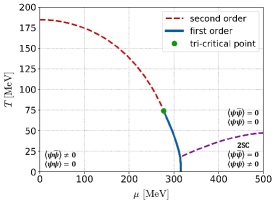
Figure 1: The phase diagram obtained in the massless 2-flavor NJL model Eq. (1). The dashed lines show the second-order phase transitions.

2 Model and phase diagram

We focus on the 2-flavor color-superconductivity (2SC), which is expected to be realized at relatively low densities, and employ the massless 2-flavor and 3-color NJL model [2, 3],

$$\mathcal{L}=\bar{\psi}i\gamma_{\mu}\partial^{\mu}\psi\ +\ G_{S}[(\bar{\psi}\psi)^{2}+(\bar{\psi}i\gamma_{5}\vec{\tau}\psi)^{2}]\ +\ G_{C}(\bar{\psi}i\gamma_{5}\tau_{2}\lambda_{A}\psi^{C})(\bar{\psi}^{C}i\gamma_{5}\tau_{2}\lambda_{A}\psi),$$ (1)

where the second and third terms represent the $qq$ and $q\bar{q}$ interactions, respectively, and $\psi^{C}(x)\equiv C\bar{\psi}^{T}(x)$ with $C=i\gamma_{2}\gamma_{0}$. $\tau_{2}$ and $\gamma_{A}$ $(A=2,5,7)$ are the antisymmetric components of the Pauli and Gell-mann matrices for the flavor $SU(2)_{f}$ and color $SU(3)_{c}$, respectively. The scalar coupling constant $G_{S}=5.01\rm{MeV^{-2}}$ and the three-momentum cutoff $\Lambda=650$ MeV are determined so as to reproduce the pion decay constant $f_{\pi}=93\rm{MeV}$ and the chiral condensate $\langle\bar{\psi}\psi\rangle=(-250\rm{MeV})^{3}$ in the chiral limit. The diquark coupling constant is set to $G_{C}=0.6G_{S}$. We show the phase diagram obtained in the mean-field approximation (MFA) with the mean fields $\langle\bar{\psi}\psi\rangle$ and $\langle\bar{\psi}^{C}i\gamma_{5}\tau_{2}\lambda_{A}\psi\rangle$ in Fig. 1. The 2SC phase is realized at low temperature and high density region. In the following, we focus on the medium near but above the critical temperature of 2SC.

3 Photon self-energy due to the diquark fluctuations

The dilepton production rate is given in terms of the retarded photon self-energy $\Pi^{R\mu\nu}(k)$ as

$$\frac{d^{4}\Gamma}{d^{4}k}=\frac{\alpha}{12\pi^{4}}\frac{1}{k^{2}}\frac{1}{e^{\beta\omega}-1}g_{\mu\nu}{\rm Im}\Pi^{R\mu\nu}(k),$$ (2)

where $k=(\bm{k},\omega)$ is the four momentum of the photon and $\alpha$ is the fine structure constant.

In Refs. [2, 3], it has been pointed out that the diquark fluctuations develop the collectivity at temperatures above but near the critical temperature of the CSC. In the present study we investigate the modification of the photon self-energy due to the diquark fluctuations. The photon self-energy is derived so that it satisfies the Ward-Takahashi (WT) identity $k_{\mu}\Pi^{R\mu\nu}(k)=0$ utilizing the thermodynamic potential.

3.1 Diquark fluctuation mode

Figure 2: Diagrammatic representation for the propagator Eq. (3).

The propagator of the diquark fluctuations in the random-phase approximation (Fig. 2) is given by

$$\Xi(\bm{q},i\nu_{n})=\frac{G_{C}}{1+G_{C}\mathcal{Q}(\bm{q},i\nu_{n})},$$ (3)

where $\mathcal{Q}(\bm{q},i\nu_{n})$ is the one-loop quark-quark correlation

$$\mathcal{Q}(\bm{q},i\nu_{n})=-2N_{f}(N_{c}-1)T\sum_{m}\int\frac{d^{3}p}{(2\pi)^{3}}{\rm Tr}[C\Gamma\mathcal{G}_{0}(\bm{q-p},i\nu_{n}-i\omega_{m})\Gamma C\mathcal{G}_{0}^{T}(\bm{p},i\omega_{m})],$$ (4)

$\omega_{m}$ ($\nu_{n}$) is the Matsubara frequency for fermions (bosons), ${\rm Tr}$ is the trace over the Dirac indices and $\mathcal{G}_{0}(\bm{p},i\omega_{m})=1/[(i\omega_{m}+\mu)\gamma_{0}-\bm{q}\cdot\bm{\gamma}]$ is the free quark propagator. By taking the analytic continuation $\Xi^{R}(\bm{q},\omega)=\Xi(\bm{q},i\nu_{n}\rightarrow\omega+i\eta)$ one obtains the retarded propagator. We remark that $[\Xi^{R}(\bm{0},0)]^{-1}=0$ is satisfied at $T=T_{c}$ determined by the MFA, which is nothing but the Thouless criterion for determining the critical temperature of the second-order phase transition. The Thouless criterion shows that the diquark propagator $\Xi^{R}(\bm{q},\omega)$ has a pole at the origin at $T=T_{c}$, and hence the diquark fluctuations have the properties of the soft mode [2, 3].

3.2 Photon self-energy

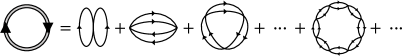
Figure 3: Contribution of the diquark fluctuations to the thermodynamic potential.

To incorporate the effects of the diquark fluctuations into the photon self-energy in a form that satisfies the WT identity, we start from the one-loop diagram of $\Xi(\bm{q},i\nu_{n})$ shown in Fig. 3, i.e. the lowest contribution of diquark fluctuations to the thermodynamic potential. The photon self-energy is then constructed by attaching electromagnetic vertices at two points of quark lines in Fig. 3. One then obtains four types of diagrams shown in Fig. 4. These diagrams are called the Aslamasov-Larkin (AL) (Fig. 4(a)) [5], Maki-Thompson (MT) (Fig. 4(b)) [6] and density of states (DOS) (Fig. 4(c, d)) [7] terms in the theory of metallic superconductivity. Each contribution to the photon self-energy, $\Pi_{\rm AL}^{\mu\nu}(k)$, $\Pi_{\rm MT}^{\mu\nu}(k)$ and $\Pi_{\rm DOS}^{\mu\nu}(k)$, respectively, is given by

$$\Pi_{\rm AL}^{\mu\nu}(k) =4N_{c}\ T\sum_{n}\int\frac{d^{3}q}{(2\pi)^{3}}\Gamma^{\mu}(q,q+k)\Xi(q+k)\Gamma^{\nu}(q+k,q)\Xi(q),$$ (5)

$$\Pi_{\rm MT}^{\mu\nu}(k) =2N_{c}\ T\sum_{n}\int\frac{d^{3}q}{(2\pi)^{3}}\Xi(q)R_{\rm MT}^{\mu\nu}(q,k),$$ (6)

$$\Pi_{\rm DOS}^{\mu\nu}(k) =2N_{c}\ T\sum_{n}\int\frac{d^{3}q}{(2\pi)^{3}}\Xi(q)R_{\rm DOS}^{\mu\nu}(q,k),$$ (7)

with

$$\Gamma^{\mu}(q,q+k) =2N_{f}(N_{c}-1)\ T\sum_{m}\int\frac{d^{3}p}{(2\pi)^{3}}{\rm Tr}[\mathcal{G}_{0}(p)\gamma^{\mu}\mathcal{G}_{0}(p+k)\mathcal{G}_{0}(q-p)],$$

$$R_{\rm MT}^{\mu\nu}(q,k) =2N_{f}(N_{c}-1)\ T\sum_{m}\int\frac{d^{3}p}{(2\pi)^{3}}{\rm Tr}[\mathcal{G}_{0}(p)\gamma^{\mu}\mathcal{G}_{0}(p+k)\mathcal{G}_{0}(q-p-k)\gamma^{\nu}\mathcal{G}_{0}(q-p)],$$

$$R_{\rm DOS}^{\mu\nu}(q,k) =2N_{f}(N_{c}-1)\ T\sum_{m}\int\frac{d^{3}p}{(2\pi)^{3}}\Big{\{}{\rm Tr}[\mathcal{G}_{0}(p)\gamma^{\mu}\mathcal{G}_{0}(p+k)\gamma^{\nu}\mathcal{G}_{0}(p)\mathcal{G}_{0}(q-p)]$$

$$\qquad\qquad\qquad\qquad\qquad\qquad\quad+{\rm Tr}[\mathcal{G}_{0}(p)\gamma^{\mu}\mathcal{G}_{0}(p-k)\gamma^{\nu}\mathcal{G}_{0}(p)\mathcal{G}_{0}(q-p)]\Big{\}}.$$

The total photon self-energy is then given by

$$\Pi^{\mu\nu}(k)=\Pi_{\rm free}^{\mu\nu}(k)+\Pi_{\rm fluc}^{\mu\nu}(k),\qquad\Pi_{\rm fluc}^{\mu\nu}(k)=\Pi_{\rm AL}^{\mu\nu}(k)+\Pi_{\rm MT}^{\mu\nu}(k)+\Pi_{\rm DOS}^{\mu\nu}(k)$$ (8)

where $\Pi^{\mu\nu}_{\rm free}(k)$ is the self-energy of the free quark system and $\Pi^{\mu\nu}_{\rm fluc}(k)$ denotes the modification of the self-energy due to the diquark fluctuations. One can explicitly check that Eq. (8) satisfies the WT identity.

(a)

(b)

(c)

(d)

Figure 4: Diagrammatic representations of the Aslamasov-Larkin (a), Maki-Thompson (b) and density of states (c,d) terms in Eqs. (5)–(7). The wavy lines represent photons.

3.3 Time-dependent Ginzburg-Landau (TDGL) approximation

The diagrams in Fig. 4 involve three-loop momentum integrals, which are cumbersome to compute. Therefore, we employ an approximation that incorporates essential effects of the diquark fluctuations near $T_{c}$ but, at the same time, allows us to evaluate the diagrams with a relative ease.

Since $[\Xi^{R}(\bm{0},0)]^{-1}=0$ at $T=T_{c}$ by the Thouless criterion, $\Xi^{R}(\bm{q},\omega)$ in the low energy-momentum region may be well approximated near but above $T_{c}$ as follows,

$$\Xi^{R}(\bm{q},\omega)=\frac{G_{C}}{c_{0}\omega+c_{1}\bm{q}^{2}+a},$$ (9)

where the coefficients $c_{0}$, $c_{1}$ and $a$ can have $T$ dependence and $a=0$ at $T=T_{c}$ from the Thouless criterion. We determine these coefficients as $a=G_{C}[\Xi^{R}(\bm{0},0)]^{-1}$, $c_{0}=G_{C}(\partial/\partial\omega)[\Xi^{R}(\bm{0},0)]^{-1}$ and $c_{1}=G_{C}(\partial/\partial\bm{q}^{2})[\Xi^{R}(\bm{0},0)]^{-1}$ from $\Xi^{R}(\bm{q},\omega)$ obtained in the NJL model. It is found that $c_{0}$ is complex while $c_{1}$ and $a$ real numbers. The approximation Eq. (9) is called the time-dependent Ginzburg-Landau (TDGL) approximation in literature. In Ref. [3], it has been shown that Eq. (9) reproduces the behavior of $\Xi^{R}(\bm{q},\omega)$ over wide ranges of $\omega$, $\bm{q}^{2}$ and $T(>T_{c})$.

Next we consider similar approximations for the vertex functions $\Gamma^{\mu}(q,q+k)$ and $R^{\mu\nu}(q,k)=R_{\rm MT}^{\mu\nu}(q,k)+R_{\rm DOS}^{\mu\nu}(q,k)$. Here, we consider such approximations only for the spatial components of these vertices because Eq. (2) can be obtained only with the spatial components of $\Pi^{R\mu\nu}(k)$; although Eq. (2) contains $\Pi^{00}(k)$, this term is expressed in terms of the longitudinal part as $\Pi^{R00}(k)=\bm{k}^{2}\Pi^{R11}(k)/k_{0}^{2}$ with $k=(k_{0},|\bm{k}|,0,0)$ from the WT identity. To approximate the spatial components $\Gamma^{i}(q,q+k)$ and $R^{ij}(q,k)$ to be consistent with Eq. (9), we substitute Eq. (9) into the WT identities for these vertices

$$k_{\mu}\Gamma^{\mu}(q,q+k)=\Xi^{-1}(q+k)-\Xi^{-1}(q),$$ (10)

$$k_{\mu}R^{\mu\nu}(q,k)=2[\Gamma^{\nu}(q-k,q)-\Gamma^{\nu}(q,q+k)].$$ (11)

Then, by comparing the lowest order terms of $\bm{q}$ and $\bm{k}$ in Eqs. (10) and (11) we obtain

$$\Gamma^{i}(q,q+k)=\frac{\partial\Xi^{-1}(q+k)}{\partial k_{i}}=\frac{c_{1}}{G_{C}}(2q+k)^{i},\quad R^{ij}(q,k)=2\frac{\partial\Gamma^{j}(q,q-k)}{\partial k_{i}}=-\frac{4c_{1}}{G_{C}}\frac{k^{i}k^{j}}{\bm{k}^{2}}.$$ (12)

Each vertex in Eq. (12) is real, and this fact simplifies the analytic continuation to obtain the retarded self-energy. One also finds that the imaginary part of $\Pi^{Rij}_{\rm MT}(q)+\Pi^{Rij}_{\rm DOS}(q)$ calculated with Eqs. (9) and (11) vanishes. Therefore, the MT and DOS terms do not contribute to the dilepton production rate. This is in accordance with the case of the metallic superconductivity [7].

4 Numerical results of dilepton production rate

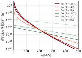
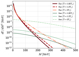
Figure 5: The dilepton production rates per unit energy $\omega$ at $\bm{k}=0$ (left) and per invariant mass $M$ (right). In each panel, the thick (red) lines are the contribution of diquark fluctuations $\Pi^{\mu\nu}_{\rm fluc}(k)$, and the thin (green) lines are the results for the free quark gas. The solid, dashed and dash-dotted lines are the results for $T=1.05T_{c}$, $1.2T_{c}$ and $2T_{c}$.

In Fig. 5, we show the dilepton production rate Eq. (2) calculated from the photon self-energy Eq. (8) at the quark chemical potential $\mu=350$ MeV for several values of $T$ above $T_{c}$. Shown in the left panel is the production rate per unit energy at $\bm{k}=0$. The thick (red) lines show the contribution of diquark fluctuations $\Pi_{\rm fluc}^{\mu\nu}(k)$, while the thin (green) lines are the results for free quarks obtained from $\Pi_{\rm free}^{\mu\nu}(k)$. The total rate is given by the sum of these two contributions. The figure shows that the production rate from the diquark fluctuations is greatly enhanced in the low energy region compared with the free quark gas for $T\lesssim 2T_{c}$, and this enhancement is more pronounced as the system is closer to the critical temperature $T_{c}$. This is not unexpected because the diquark fluctuations are the soft mode which acquires more concentrated strength in the vicinity of the critical point. In the right panel, we show the invariant-mass ($M$) spectrum

$$\frac{d\Gamma}{dM^{2}}=\frac{1}{2\omega}\int d^{3}k\frac{d^{4}\Gamma}{d^{4}k},$$ (13)

which is more convenient for a comparison with experimental data. One sees that the enhancement of the production rate at small $M$ is observed in the invariant-mass spectrum for a similar temperature range, while the $T$ dependence of the enhancement is milder than the left panel.

5 Summary and concluding remarks

In this study, we investigated the effect of diquark fluctuations on the dilepton production rate near but above the critical temperature of the 2SC. The contribution of the diquark fluctuations was taken into account so as to satisfy the WT identity in the TDGL approximation. It was found that the dilepton production rate is greatly enhanced in comparison to the free-quark gas case in the low energy and low invariant-mass regions near $T_{c}$. This result suggests that such an enhancement can be used for the experimental signal for the existence of the CSC phases. In particular, the fact that the enhancement is seen even at $T\simeq 2T_{c}$ would allow us to detect the signal in the HIC experiments even when $T_{c}$ is so small that the realization of the CSC phase itself in the HIC is impossible.

References

• [1] M. G. Alford, A. Schmitt, K. Rajagopal and T. Schäfer, Rev. Mod. Phys. 80 (2008), 1455.
• [2] M. Kitazawa, T. Koide, T. Kunihiro and Y. Nemoto, Phys. Rev. D 65 (2002), 091504.
• [3] M. Kitazawa, T. Koide, T. Kunihiro and Y. Nemoto, Prog. Theor. Phys. 114 (2005), 117.
• [4] T. Kunihiro, M. Kitazawa and Y. Nemoto, PoS CPOD07 (2007), 041.
• [5] L. G. Aslamasov and A. L. Larkin, Sov. Phys. -Solid State 10 (1968), 875.
• [6] K. Maki, Prog. Theor. Phys. 40 (1968), 193; R. S. Thompson, Phys. Rev. B 1 (1970), 327.
• [7] A. I. Larkin and A. A. Varlamov, Fluctuation Phenomena in Superconductors (Springer Berlin Heidelberg, 2008).