A fractional glance to the theory of edge dislocations

Abstract.

We revisit some recents results inspired by the Peierls-Nabarro model on edge dislocations for crystals which rely on the fractional Laplace representation of the corresponding equation. In particular, we discuss results related to heteroclinic, homoclinic and multibump patterns for the atom dislocation function, the large space and time scale of the solutions of the parabolic problem, the dynamics of the dislocation points and the large time asymptotics after possible dislocation collisions.

1. Introduction

1.1. The Peierls-Nabarro model for edge dislocations

The theory of edge dislocations describes defects in the atoms display of a crystal structure. In a nutshell, dislocations represent areas of a crystal in which the atoms do not lie in the geometrically organized pattern of the material, and they are responsible for plastic deformations to occur. In particular, these plastic deformations occur without altering the chemical composition of the material and under external forces significantly lower than expected.

As an example of dislocation, one can think of a simple cubic lattice representing the crystal at a large scale and suppose that an irregularity arises in the lattice: see for instance Figure 1, in which an imperfection of the crystal is visible on the fourth horizontal row.

As a matter of fact, Figure 1 must be understood as (the local reproduction of) a planar section of a three-dimensional (infinitely extended) crystal and represents the “typical” anomaly associated to an edge dislocation, as being caused by the termination of a plane of atoms in the middle of a crystal (the picture is similar to that of sticking half of a piece of paper into a stack of paper; in this case the half of a piece of paper corresponding to the three extra atoms visible in the upper part of the third column of atoms in Figure 1).

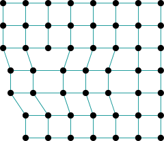
Figure 1. A defect in a crystal (the black dots corresponding to atoms and the cyan segments to the bonds between atoms).

A pioneer description of elastic dislocations dates back to Vito Volterra [MR1509085] and the connection between plastic deformations and dislocation theory was set forth by Egon Orowan, Michael Polanyi and Geoffrey Taylor (independently and at about the same time) explaining that the stress needed for the slip was far lower than theoretical predictions in view of the theory of dislocations [ORO1, ORO2, ORO3, POLA, zbMATH02539109, zbMATH02539110]. An intuitive reason for why dislocation dynamics allow plastic displacements under a low external force can be found by comparing this phenomenon with the amusing locomotion of caterpillars obtained by squeezing muscles in sequence in an undulating wave motion: namely, since caterpillars do not have any bone in their entire bodies, they can produce a “defect” by arching their body and obtain a displacement by moving this defect along their body (this is however a rather crude biological explanation, if interested in a detailed analysis of the caterpillars’ locomotion see e.g. [VAN]).

At that time, the description of dislocations was mainly based on theoretical predictions with little or no experimental evidence for dislocations. Indeed, although slip lines on the surface of metals had been observed by optical microscopy, a direct observation of crystal dislocations arrived later, since it required transmission electron microscopes [VERMA, AME, BOL, HIR0, Silcox1959-SILDOO-2, HIR].

A useful graphical device to detect crystal defects in a lattice is given by the so-called Burgers vector, named after Johannes (Jan) Martinus Burgers [BUR], see Figure 2. The gist is that in a perfect crystal structure if one moves for a given number of steps, say three, in every coordinate direction, say right-down-left-up, the trajectory produced is a square that returns to the initial point; instead, when a similar ideal movement is drawn encompassing a dislocation, the arrival point is different from the initial one and the vector joining the starting position with the final one is a vector, namely the Burgers vector, which encodes the magnitude and direction of the crystal imperfection.

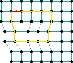
Figure 2. Burgers vector.

From the static viewpoint, a crystal defect produces a structural inhomogeneity corresponding e.g. in Figure 1 to a relative compression above the dislocation, a relative tension below and a shear on the side (the shear can be visualized since the bonds between atoms are shaped in the form of a parallelogram rather than a regular square).

In practice, one can take advantage of this structural imperfection by producing plastic deformations as an outcome of the motion of dislocations which is induced by a set of shearing forces, namely forces parallel to one of the axis of the lattice, pushing the crystal in one specific direction from a side, and in the opposite direction from the other side (whatever “side” may mean here, since our ideal crystal has infinite extension in every direction). See Figure 3 for a description of shearing forces.

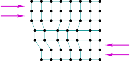
Figure 3. Shearing forces.

The advantage of dislocations towards plastic deformations is that when the shearing forces are parallel to the Burgers vector their result can be that of weakening or breaking some of the bonds between atoms and allow them to slide over each other. This glide, or slip, method is thus capable of producing plastic deformations at low stress levels. See Figure 4 for a cartoon of how a shearing force can move around dislocations in the lattice with the final outcome of producing a visible plastic deformation: the idea is that by conveniently sliding a dislocation the crystalline order is restored on either side but the atoms on one side have moved by one position.

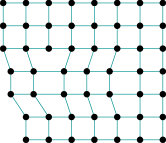
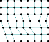
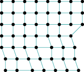
$\mapsto$ $\mapsto$ $\mapsto$

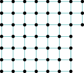
Figure 4. Plastic deformation as an outcome of crystal dislocation motion.

We have a direct experience of the role played by dislocations in plastic deformations anytime we indulge in playing around with paperclips (those little devices made of steel wire bent to a looped shape that we use to hold sheets of paper together before every useful information was digitalized and posted on the internet, see Figure 5): with soft movements of our fingers, we can easily open and close repeatedly the looped shape of a paperclip, enjoying its flexibility and malleability – till at some point the paperclip becomes suddenly quite stiff and to change its shape we need to exert some extra force which typically ends up breaking the paperclip. Hence, this simple experiment somehow confirms how the strength and ductility of metals are influenced and controlled by dislocations.

Figure 5. A few paper clips of different colors (Public Domain image from Wikipedia).

The physical explanation of this phenomenon is that at the beginning the paperclip structure presents some defects and our soft movements rely on the dynamics of these dislocations to modify the shape of the object; at some point, however, several of these imperfections get resolved precisely by our repeated opening and closing the loop of the clip, and when no more dislocation is available (or when too few dislocations are available) the perfect (or almost perfect) lattice offers a sounder resistance to the external stress (see the last frame in Figure 4), which results in the (perhaps not so expected) stiffness that typically make this game end by the breaking of the clip.

Some technical remarks are in order. First off, the assumption that the crystal has a simple cubic structure (also called primitive cubic in jargon) is indeed a great geometric simplification but it includes several concrete cases of interest, such as polonium ${\rm Po}$, see [PLON], iron pyrite ${\rm FeS_{2}}$, see Figure 6, as well as an allotrope of selenium ${\rm Se}$, see [SELE].

Figure 6. Pyrite cubic crystals (image from Wikipedia, licensed under the Creative Commons Attribution-Share Alike 3.0 Unported license).

Furthermore, we stress that we are focused here on edge dislocations, namely we only consider here situations in which dislocations move in the direction of the Burgers vector (as in Figures 3, 4 and 7). Other situations also occur in nature, such as the so-called screw dislocations in which the dislocation dynamics takes place in a direction perpendicular to the Burgers vector, thus creating a helical arrangement of atoms around the core, see e.g. Figure 8. Mixed dislocations exist as well, in which case the Burgers vector is neither parallel nor orthogonal to the dislocation dynamics. But in this note we confine our interest to the simplest case of edge dislocations.

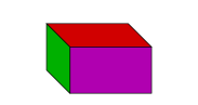
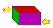
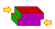
$\mapsto$ $\mapsto$ $\mapsto$

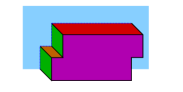
Figure 7. Slip of a crystal along a horizontal plane in an edge dislocation, and vertical section.

To mathematically describe edge dislocations, we recall the classical model by Rudolf Peierls and Frank Nabarro. Suppose that the crystal is subject to shearing forces causing a slip along a horizontal plane, that we call the slip plane. We take a vertical section of the crystal, see Figure 7. The intersection between the horizontal slip plane and the vertical sectional plane is called slip line. We suppose that at a large scale the crystal has a simple cubic structure described by the lattice $\mathbb{Z}^{3}$ and accordingly the vertical sectional plane is such that it detects a large scale atom disposition described by the lattice $\mathbb{Z}^{2}$.

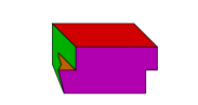
Figure 8. A screw dislocation.

We stress that this lattice does not describe the position of every single atom, since defects at small scales can occur. The dislocation theory thus makes the ansatz that the lattice structure simply dictates a favorable state for atoms which are however free to move, subject to a potential that penalizes the atom positions outside the lattice structure and a bond interaction between atoms.

The slip will indeed cause some misalignment between the atoms below the slip lines and the ones above. For concreteness, we focus our attention on the atoms above the slip line (the case of the ones below being similar) and we aim at describing their mismatch with respect to the lattice structure.

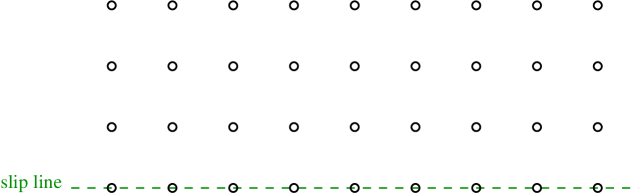
Figure 9. Rest position of the atoms corresponding to the large scale crystalline structure.

For this, we consider the atom rest positions $\mathbb{Z}^{2}$ in the upper halfplane $\mathbb{R}\times[0,+\infty)$, corresponding to the empty circles in Figure 9.

Positions in this halfplane are denoted by using coordinates $(x,y)\in\mathbb{R}\times[0,+\infty)$. The position of each atom is described by a dislocation function that identifies the mismatch with respect to the rest position: for simplicity, we assume that atoms can only slide horizontally (that is, parallel to the slip plane and to the shearing forces), see Figure 10 in which the full circles represent the atoms (we are thus neglecting the vertical mismatch of atoms possibly caused by mutual bonds, by considering this effect as negligible with respect to the shearing force).

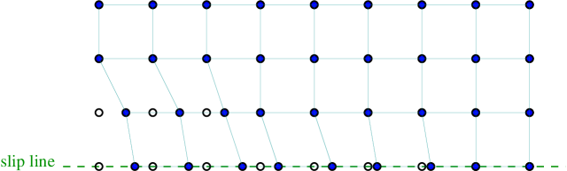
Figure 10. Mismatch between atom location and crystal structure.

In this setting, the distance between the actual position of an atom and its rest position located at $(x,y)\in\mathbb{R}\times[0,+\infty)$ corresponds to a scalar function $U(x,y)$ (say, with $U$ positive if the atom is dislocated towards the right and negative if the atom is dislocated towards the left, see Figure 11). It is also convenient to consider the trace of the dislocation function $U$ along the slip line which corresponds to $u(x):=U(x,0)$.

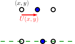
Figure 11. The dislocation function $U(x,y)$.

In a situation such as the one described in Figure 7, we can argue that most of the mismatch occurs along the slip line: roughly speaking, we can expect the atoms located in the upper halfplane to be mostly alligned with a cubic lattice and the ones located in the lower halfplane to be mostly alligned with another cubic lattice which is a horizontal translation of the previous one. Therefore, we can suppose that the main contribution to the crystal mismatch is encoded by the function $u$. To quantify this mismatch, we consider a multiwell potential $W$, say a scalar function such that $W(k)=0$ for all $k\in\mathbb{Z}$ and $W(r)>0$ for all $r\in\mathbb{R}\setminus\mathbb{Z}$. For simplicity, we will suppose in what follows that $W$ is smooth, periodic of period $1$, even and such that $W^{\prime\prime}(0)\neq 0$.

This potential penalizes atoms which are not aligned with the lattice structure, since $W(u(x))$ turns out to be positive unless $u(x)\in\mathbb{Z}$, that is unless the atom with ideal rest position at $x$ is located to a point of the lattice (recall that any point of the lattice ends up to be good for the atom to be in equilibrium with respect to the large scale structure of the crystal).

As a result, in this model the total energy contribution coming from atom displacement can be written as

$${\mathcal{P}}(U):=\int_{\mathbb{R}}W(u(x))\,dx.$$

The total energy however has to account also for the bonds between atoms. The simplest ansatz is to suppose that this energy contribution resembles an elastic energy of the form

(1.1) $${\mathcal{E}}(U):=\frac{1}{2}\int_{\mathbb{R}\times(0,+\infty)}|\nabla U(x,y)|^{2}\,dx\,dy,$$

where the factor $\frac{1}{2}$ has been introduced for later convenience (we are disregarding here structural constants).

The total energy is therefore the sum of the displacement energy and the bond energy and takes the form

$${\mathcal{H}}(U):={\mathcal{E}}(U)+{\mathcal{P}}(U)=\frac{1}{2}\int_{\mathbb{R}\times(0,+\infty)}|\nabla U(x,y)|^{2}\,dx\,dy+\int_{\mathbb{R}}W(u(x))\,dx.$$

We stress that this model is, in a sense, of “hybrid” type: while the rest position of the atoms correspond to a lattice structure with a discrete feature, the dislocation function $U$ (and thus its trace $u$) is assumed to be continuous (and actually smooth) and defined in the continuum given by $\mathbb{R}\times(0,+\infty)$. This “philosophical inconsistency” between the discrete and continuous descriptions of nature is compensated by a simple and effective realization of the model and it is also, at least partially, justified by the fact that the atom distance is typically much smaller than the plastic effects that one is interested in taking into account (therefore, for practical purposes, the lattice acting as a substratum is “almost” a continuum).

Equilibrium configurations of this model correspond to critical points of ${\mathcal{H}}$. These configurations can be detected by noticing that, for every $R>0$ and any smooth function $\Psi:\mathbb{R}\times[0,+\infty)\to\mathbb{R}$ such that $\Psi(x,y)=0$ if $|(x,y)|\geqslant R$,

(1.2) $$\begin{split}0&=\langle D{\mathcal{H}}(U),\Psi\rangle\\ &=\int_{\mathbb{R}\times(0,+\infty)}\nabla U(x,y)\cdot\nabla\Psi(x,y)\,dx\,dy+\int_{\mathbb{R}}W^{\prime}(u(x))\psi(x)\,dx\\ &=-\int_{\mathbb{R}\times(0,+\infty)}\Delta U(x,y)\Psi(x,y)\,dx\,dy+\int_{\mathbb{R}}\big{(}W^{\prime}(u(x))-\partial_{y}U(x,0)\big{)}\psi(x)\,dx,\end{split}$$

where $\psi(x):=\Psi(x,0)$, thanks to Green’s first identity.

In particular, if we take a ball $B\Subset\mathbb{R}\times(0,+\infty)$ and a function $\Psi_{0}\in C^{\infty}_{0}(B)$, it follows that $\psi_{0}(x):=\Psi_{0}(x,0)=0$ for all $x\in\mathbb{R}$ and thus, by (1.2),

$$0=-\int_{\mathbb{R}\times(0,+\infty)}\Delta U(x,y)\Psi(x,y)\,dx\,dy,$$

that leads to $U$ being harmonic in $\mathbb{R}\times(0,+\infty)$.

Inserting this information into (1.2), we find that

$$0=\int_{\mathbb{R}}\big{(}W^{\prime}(u(x))-\partial_{y}U(x,0)\big{)}\psi(x)\,dx,$$

giving that $W^{\prime}(u)=\partial_{y}U$ along the slip line.

From these considerations, we infer that equilibria of the Peierls-Nabarro model correspond to solutions of

(1.3) $$\begin{cases}\Delta U=0&{\mbox{ in }}\mathbb{R}\times(0,+\infty),\\ \partial_{y}U=W^{\prime}(u)&{\mbox{ in }}\mathbb{R}\times\{0\}.\end{cases}$$

Formally, using the harmonicity of $U$ and the Poisson kernel for the halfspace, we thus obtain that, for all $(x,y)\in\mathbb{R}\times(0,+\infty)$,

$$U(x,y)=\frac{1}{\pi}\int_{\mathbb{R}}\frac{y\,u(\zeta)}{(x-\zeta)^{2}+y^{2}}\,d\zeta.$$

To remove the singularity as $y\searrow 0$, one can notice that a primitive of $\mathbb{R}\ni\zeta\mapsto\frac{y}{(x-\zeta)^{2}+y^{2}}$ is $\arctan\left(\frac{\zeta-x}{y}\right)$ and accordingly

$$\frac{1}{\pi}\int_{\mathbb{R}}\frac{y}{(x-\zeta)^{2}+y^{2}}\,d\zeta=\frac{1}{\pi}\big{(}\arctan(+\infty)-\arctan(-\infty)\big{)}=1.$$

This gives that

$$U(x,y)-u(x)=\frac{1}{\pi}\int_{\mathbb{R}}\frac{y\,\big{(}u(\zeta)-u(x)\big{)}}{(x-\zeta)^{2}+y^{2}}\,d\zeta$$

and therefore

$$W^{\prime}(u(x))=\lim_{y\searrow 0}\partial_{y}U(x,y)=\lim_{y\searrow 0}\partial_{y}\big{(}U(x,y)-u(x)\big{)}=\frac{1}{\pi}\lim_{y\searrow 0}\int_{\mathbb{R}}\frac{\partial}{\partial y}\left(\frac{y\,\big{(}u(\zeta)-u(x)\big{)}}{(x-\zeta)^{2}+y^{2}}\right)\,d\zeta$$

$$\quad=\frac{1}{\pi}\lim_{y\searrow 0}\int_{\mathbb{R}}\frac{(\zeta^{2}-2x\zeta+x^{2}-y^{2})\,\big{(}u(\zeta)-u(x)\big{)}}{(\zeta^{2}-2x\zeta+x^{2}+y^{2})^{2}}\,d\zeta=\frac{1}{\pi}\int_{\mathbb{R}}\frac{u(\zeta)-u(x)}{\zeta^{2}-2x\zeta+x^{2}}\,d\zeta$$

$$\quad=\frac{1}{\pi}\int_{\mathbb{R}}\frac{u(\zeta)-u(x)}{(x-\zeta)^{2}}\,d\zeta,$$

that is, neglecting normalizing constants,

(1.4) $$-\sqrt{-\Delta}\,u=W^{\prime}(u)\quad{\mbox{ in }}\,\mathbb{R}.$$

Alternatively, one can formally obtain (1.4) from (1.3) from the analysis of a Dirichlet-to-Neumann problem (see e.g. [MR3469920, Section 4.1]) or solving the linear equation in (1.3) via Fourier transform (see e.g. [MR3469920, Section 4.3]).

We think that (1.4) is a neat example of a nonlocal equation of fractional type arising from purely classical considerations. Of course, equation (1.4) presents both advantages and disadvantages with respect to (1.3). On the one hand, equation (1.3) is classical in nature and it may seem more handy to be dealt with. On the other hand, equation (1.4) showcases the intrinsic nonlocal aspect of the problem, in which dragging one single atom along the slip line ends up influencing, in principle, the whole crystalline structure. Furthermore, equation (1.4) is set in dimension $1$, which is a considerable conceptual advantage since it opens the possibility of employing methods from dynamical systems (which will provide essential ingredients in Section 2).

Additionally, equation (1.4) immediately allows to consider more general equations of the form

(1.5) $$-(-\Delta)^{s}u=W^{\prime}(u)\quad{\mbox{ in }}\,\mathbb{R},$$

for a given $s\in(0,1)$.

In this spirit, equation (1.5) is not a mere generalization of (1.4) motivated by mathematical curiosity: instead, it can offer a useful approach to comprise models in which the range-effect of the atomic bonds is different from the one modeled by the purely elastic response introduced in (1.1). Moreover, it allows a direct comparison between equations arising in material sciences and crystal dislocation dynamics with similar ones motivated, for instance, by problems in ethology, population dynamics and mathematical biology (for instance, similar models can be considered to describe a biological population subject to a nonlocal dispersal strategy of Lévy flight type, see e.g. [GG] and the references therein).

Also, and possibly more importantly, considering (1.4) as a “particular case” of (1.5) allows one to take into account a continuous range of fractional exponents $s$, avoiding “discrete jumps” from the classical case $s=1$ (often related to the classical Allen-Cahn equation) and the case $s=\frac{1}{2}$ in (1.5): besides its conceptual advantage, this approach allows one to exploit perturbative methods in the fractional exponent (e.g. bifurcating from previously known cases).

1.2. Organization of the paper

The rest of the article is organized as follows. In Section 2 we present some recent results that describe situations in which atom dislocations in crystals can display complicated or unusual patterns as stationary equilibria, thus producing chaotic behaviors.

In Section 3 we analyze the dislocation dynamics and in Section 4 the cases in which collisions between dislocation points occur. Section 5 is then devoted to discussing what happens to the dislocations after collisions.

In Section 6 we deduce the so-called Orowan’s Law, and in Section 7 we deal with the homogenization problem associated with the Peierls-Nabarro model.

2. Chaotic dislocation displacements

A natural question is whether atom dislocations in crystals can display complicated or unusual patterns as stationary equilibria. We started the investigation of this question in [MR3594365, MR4053239]. The gist of this analysis is that, without indulging in philosophical definitions, one of the simplest forms of “chaos” consists in the possibility of producing patterns which exhibit transition layers and oscillatory behaviors. To accomplish this goal, we find it convenient to revisit some classical methods from dynamical systems and topological analysis (such as the ones in [MR1119200, MR1799055]) in light of the fractional setting introduced in (1.5).

From the technical point of view, we recall that the existing methods were designed for classical Hamiltonian or Lagrangian systems and were aiming at detecting oscillatory behaviors in the time variable, that is for the time evolution of a particle, or a system of particles. The structure in (1.5) is different, since no time variable is involved: instead, one can use methods from dynamical systems to detect oscillatory phenomena in the space variable, especially thanks to the fact that equation (1.5) is set in one space variable (after all, once things are set into a good mathematical formulation, one space variable can formally play the role of time, and vice versa).

   

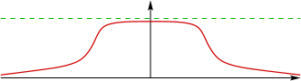
Figure 12. A heteroclinic and a homoclinic connections.

The goal in [MR3594365, MR4053239] is thus to construct complex examples of stationary equilibria for the atom dislocation function induced by a perturbation of the potential (roughly speaking, pressing or pulling a bit the crystal). The complex example that we were interested in included:

• heteroclinic connections, i.e. transition layers connecting two minima of the potential $W$,

• homoclinic connections, i.e. a nontrivial connection of a minimum of the potential $W$ to itself,

• multibump orbits, i.e. solutions oscillating somewhat arbitrarily between the minima of the potential $W$,

see Figures 12 and 13.

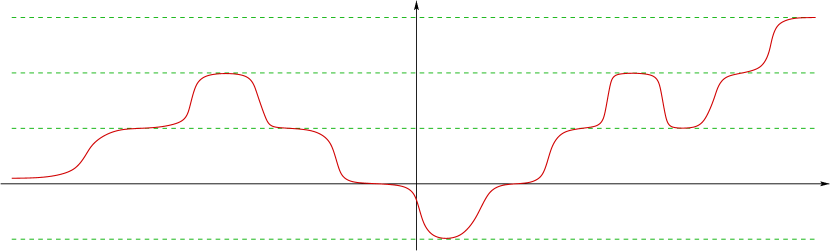
Figure 13. A multibump orbit.

To give a consistent mathematical framework to this perturbation setting, instead of (1.5) one considers the equation

(2.1) $$(-\Delta)^{s}u(x)+a(x)\,W^{\prime}(u(x))=0\qquad{\mbox{for any }}\;\,x\in\mathbb{R}.$$

The role of $a$ is that of a “generic” (arbitrarily small and with small derivatives, but nontrivial) perturbation.

Among other results, it is proved in [MR3594365] that

Theorem 1.

Let $s\in\left(\frac{1}{2},1\right)$, $N\in\mathbb{N}$, $\zeta_{1},\dots,\zeta_{N}\in\mathbb{Z}$, with $|\zeta_{i+1}-\zeta_{i}|=1$, for $i\in\{1,\dots,N-1\}$.

Then, there exist $b_{1}<\dots<b_{2N-2}\in\mathbb{R}$ and a solution $u$ of (2.1) such that:

$$\lim_{x\to-\infty}u(x)=\zeta_{1},$$

$$\sup_{x\in(-\infty,b_{1}]}|u(x)-\zeta_{1}|\leqslant\frac{1}{100},$$

$$\sup_{x\in[b_{2i},b_{2i+1}]}|u(x)-\zeta_{i+1}|\leqslant\frac{1}{100}\quad{\mbox{ for all }}i\in\{1,...,N-2\},$$

$$\sup_{x\in[b_{2N-2},+\infty)}|u(x)-\zeta_{N}|\leqslant\frac{1}{100}$$

and $$\lim_{x\to+\infty}u(x)=\zeta_{N}.$$

In this spirit, Theorem 1 constructs a spatially oscillatory equilibrium for the dislocation function as the one depicted in Figure 13: we stress that the levels $\zeta_{1},\dots,\zeta_{N}\in\mathbb{Z}$ can be prescribed arbitrarily as consecutive integers and therefore Theorem 1 states that a generic perturbation can produce dislocation patterns that oscillate essentially as one wishes; we recall that, in view of the notation stated on page 10, a positive oscillation of the dislocation function would correspond to an atom dislocation “right” with respect to its rest position, and a negative oscillation of the dislocation function would correspond to an atom dislocation “left” with respect to its rest position and accordingly the oscillations “up and down” detected in Theorem 1 would correspond to atoms arbitrarily dislocated to the left and to the right of the lattice in the setting of Section 1.1. Being able to dislocate atoms at will opens the possibility of associating to the atomic structure a “symbolic dynamics” that describes a state of the system in terms of the corresponding minimum of the potential $W$.

Particular cases of Theorem 1 include the situations displayed in Figure 12, namely:

• when $N:=2$ and $\zeta_{2}:=\zeta_{1}+1$ (or $N:=2$ and $\zeta_{2}:=\zeta_{1}-1$), one obtains a heteroclinic orbit,

• when $N:=3$ and $\zeta_{3}:=\zeta_{1}$, one obtains a homoclinic orbit.

We observe that while heteroclinic orbits also exist in case of a constant perturbation $a$, the existence of homoclinic and multibump orbits heavily depends on the fact that $a$ is supposed to be generic (and in particular nonconstant): indeed, heteroclinic orbits for constant $a$ have been constructed in [MR3081641, MR3280032] but it has been shown in [MR4108219] that no homoclinic connection and no multibump solution are possible when $a$ is constant.

The result in Theorem 1 is actually flexible enough to deal also with more general interaction kernels and with equilibria not necessarily disposed on a regular lattice. The result also applies to systems (though in this case the subsequent layer $\zeta_{i+1}$ is not completely arbitrary given $\zeta_{i}$, since it must be chosen as a suitable action minimizers among close neighbors).

In terms of methodology, while Theorem 1 takes its inspiration from classical variational methods, constrained minimization techniques and energy estimates, its proof needs to account for some of the difficulties provided by the nonlocal setting of equation (2.1). In particular:

• the “cut and paste methods” used in dynamical systems to create competitors for the energy functional and obtain energy estimates are affected in our case by nonlocality (for instance, the energy of the union of two trajectories is not the sum of their energies),

• the long tails of the solutions provide significant energy contributions (suggestively, as in what Einstein called Mach’s principle, “mass out there influences inertia here” and “local physical laws are determined by the large-scale structure of the universe” [MR0424186]).

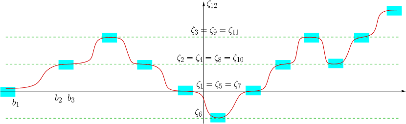
Figure 14. Constrained minimization to construct a multibump orbit.

To prove Theorem 1, the variational method relies on a constrained minimization problem: roughly speaking, one first minimizes the energy functional under the additional request that the orbit passes through suitable “windows” strategically located to create the desired oscillations (namely, the cyan boxes in Figure 14).

However, to make this argument work, one needs to avoid that the minimizing orbit constructed in this way touches the boundary of the window (indeed, if it does not, then small perturbations around the orbits are admissible and we obtain a local minimizer, hence a solution of the problem with the desired oscillations).

To get rid of the possible touching between the minimal orbit and the windows, one needs to carefully choose the intervals with endpoints $b_{1},\dots,b_{2N-2}$ and exploit the oscillations of $a$ to place the transitions in a favorable energy range.

To clarify this method, let us focus on the case of heteroclinics (which will also serve as a cornerstone to build the other kinds of trajectories), namely let us deal with the case $N:=2$ and $\zeta_{2}:=\zeta_{1}+1$. Suppose that the method of constrained minimization “goes wrong”, that is a touching occurs as shown by the magenta circle in Figure 15.

One first shows that indeed the touching point must occur quite close to the boundary of the window (at infinity, it is energetically more convenient for the solution to stay close to the minima of the potential and thus away from the window). Then, one needs to show that the transition from $\zeta_{1}$ to $\zeta_{2}$ occurs in a rather short interval (it is energetically inconvenient for the solution to stay away from the minima of the potential in a large interval). Finally, once the solution gets sufficiently close to $\zeta_{2}$ on the right, it is better for it to remain close to it (it is energetically inconvenient for the solution to drift away from the minima of the potential once it gets there).

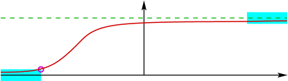
Figure 15. The constrained minimization method going wrong.

With these three ingredients in mind, we realize that indeed Figure 15 represents essentially the “worst case scenario” that we want to avoid. For this, the idea is to translate the red trajectory in Figure 15 to the right and lower its energy: to accomplish this, one needs to assume that the modulating perturbation $a$ presents some minima that we can enclose between the two cyan windows (hence, to this end, if $a$ is slowly oscillating one needs to place the windows sufficiently far from each other). Since the effect of $a$ is to modulate the potential $W$ and since we expect “most of the energy” to come from the transition from $\zeta_{1}$ to $\zeta_{2}$, it will be energetically more convenient to locate the transition inside the minima of $a$, thus obtaining a new minimizer that does not touch the window, as desired (see Figure 16).

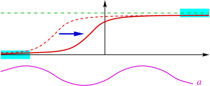
Figure 16. Translating the orbit into an energetically more favorable position.

When implementing these ideas, however, some effort is needed to take care of nonlocality, since energy competitors cannot be obtained simply by gluing pieces of trajectories (this feature will also become pivotal when one wants to address Theorem 1 in its full generality, since homoclinic and multibump solutions will be obtained precisely by “almost” glueing heteroclinics together). To minimize the impact of nonlocality on the energy computations, we glue orbits at “very flat” matching points, namely at points at which two orbits meet with very small derivative, remaining close to each other in a large interval (we quantify appropriately this notion and we call such intervals “clean intervals”). The existence of these clean intervals is obtained by combining energy estimates and fractional elliptic regularity theory.

We observe that Theorem 1 was obtained in the fractional exponent range $s\in\left(\frac{1}{2},1\right)$ which is arbitrarily close to, but different from, the exponent $s=\frac{1}{2}$ arising in (1.4). The case $s=\frac{1}{2}$, or more generally $s\in\left(0,\frac{1}{2}\right]$, is indeed quite challenging, due to several additional difficulties. First of all, when $s=\frac{1}{2}$ one has to account for unbounded competitors, namely functions with finite energy and unbounded spikes (which would make the constrained minimization problem with pointwise windows unpractical). To appreciate this hindrance, one may consider the function

$$\bar{\psi}(x):=\chi_{(-1,1)}(x)\ln(1-\ln|x|)$$

which belongs to $H^{1/2}(\mathbb{R})\setminus L^{\infty}(\mathbb{R})$, see [MR4053239, Appendix A]. From this, one can easily construct competitors with small energy but unbounded spikes, e.g. both accumulating at some given points and at infinity, such as

$$\bar{\psi}_{\varepsilon}(x):=\varepsilon\sum_{k\in\mathbb{Z}}\frac{\bar{\psi}\big{(}2^{|k|}(x-2^{k})\big{)}}{2^{|k|}},$$

see Figure 17.

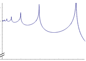
Figure 17. A small energy competitor with many unbounded spikes.

An additional difficulty comes from the fact that when $s=\frac{1}{2}$ heteroclinic solutions have infinite energy: to appreciate this, one can argue that, roughly speaking, if

(2.2) $$u_{\star} u_{\star}(-\infty)=0 u_{\star}(+\infty)=1$$ solves (1.5) and is monotone and such that  and ,

then, setting $w:=u^{\prime}_{\star}$, at $+\infty$ one obtains a behavior of the type

$$-(-\Delta)^{s}w(x)=W^{\prime\prime}(u_{\star}(x))w(x)\simeq W^{\prime\prime}(1)w(x),$$

that is, for large $x$,

$$w(x)\simeq\int_{\mathbb{R}}\frac{w(\zeta)-w(x)}{|x-\zeta|^{1+2s}}\,d\zeta\simeq\int_{\mathbb{R}}\frac{w(\zeta)}{|x-\zeta|^{1+2s}}\,d\zeta\simeq\frac{C}{x^{1+2s}}$$

and consequently

(2.3) $$u_{\star}(x)\simeq 1-\frac{C}{x^{2s}}.$$

This shows that when $s=\frac{1}{2}$, and more generally when $s\in\left(0,\frac{1}{2}\right]$, the heteroclinics possess infinite elastic energy, because, for large $R$,

$$\iint_{\mathbb{R}\times\mathbb{R}}\frac{|u_{\star}(x)-u_{\star}(y)|^{2}}{|x-y|^{1+2s}}\,dx\,dy\geqslant\frac{1}{4}\iint_{(R,+\infty)\times(-\infty,-R)}\frac{dx\,dy}{(x-y)^{1+2s}}=\frac{1}{8s}\int_{(R,+\infty)}\frac{1}{(x+R)^{2s}}\,dx=+\infty.$$

These observations clarify that for $s=\frac{1}{2}$, and more generally for $s\in\left(0,\frac{1}{2}\right]$, the standard variational methods need to be modified since the objects that we seek have infinite energy while the objects that we want to avoid (such as the ones presenting uncontrolled spikes) can have finite, and even small, energy.

These difficulties have been addressed in [MR4053239], where heteroclinic connections for equation (2.1) have been constructed in the fractional exponent range $s\in\left(\frac{1}{4},\frac{1}{2}\right]$. To overcome the difficulty arising from the infinite energy of the heteroclinics, we use “energy renormalization” methods (by formally subtracting the infinite elastic energy of the heteroclinic to the functional). Also, to avoid finite energy competitors which may be discontinuous, and even unbounded, we employe an “energy penalization” method, by adding a “viscosity” term to the equation, obtaining uniform estimates via elliptic theory (actually, via a combination of classical and fractional elliptic theories). For this, an important step is to detect how the constrained minimizers detach from the windows: namely, since the energy by itself cannot guarantee continuity in this fractional exponent range, one needs an auxiliary argument to avoid that minimizers “jump” away when touching the boundary of the constraints. These detachment estimates are obtained from the analysis of the corresponding obstacle problem (the window playing the role of the obstacle at detaching points).

Another technical issue in this fractional exponent range is that approximating heteroclinics may oscillate between equilibria when placing the windows far from each other: to avoid this pathology, we use a second penalization method to charge the $L^{2}$-difference with a centered excursion, so to control the “baricenter” of the heteroclinic.

3. Dislocation dynamics

To understand the way in which dislocations move, one can look at the parabolic analogue of equation (1.5), namely consider solutions $v=v(t,x)$ of

(3.1) $$\partial_{t}v=-(-\Delta)^{s}v-W^{\prime}(v)\quad{\mbox{ in }}\,(0,+\infty)\times\mathbb{R}.$$

More generally, one can consider the equation

$$\partial_{t}v=-(-\Delta)^{s}v-W^{\prime}(v)+\sigma_{\varepsilon},$$

where $\sigma_{\varepsilon}$ is a suitably small external stress, but to keep the exposition as simple as possible we take here $\sigma_{\varepsilon}\equiv 0$.

In this section, we recall some results aiming at describing the evolution of the parabolic dislocation function $v$ for suitably large space and time scales. To accomplish this goal, it is appropriate to scale both the space and the time variables according to the homogeneity of the equation, that is considering the function

(3.2) $$v_{\varepsilon}(t,x):=v\left(\frac{t}{\varepsilon^{1+2s}},\frac{x}{\varepsilon}\right).$$

Here $\varepsilon>0$ is a small parameter: sending $\varepsilon\searrow 0$ would thus correspond to considering large time and space scales, in a suitably intertwined manner that detects a coherent pattern.

By scaling (3.1), one obtains the evolution equation for $v_{\varepsilon}$ given by

(3.3) $$\varepsilon\partial_{t}v_{\varepsilon}=-(-\Delta)^{s}v_{\varepsilon}-\frac{1}{\varepsilon^{2s}}W^{\prime}(v_{\varepsilon})\quad{\mbox{ in }}\,(0,+\infty)\times\mathbb{R}.$$

Since the dynamics of the atom dislocations can be quite complicated, it is also convenient to take into account “well-prepared” initial data, obtained by the superposition of transition layers. That is, we consider the heteroclinic solution $u_{\star}$ constructed in [MR3081641, MR3280032] and mentioned in (2.2) (normalized such that $u_{\star}(0)=\frac{1}{2}$): this will be the transition layer (from $0$ to $1$) used as a building block for our construction. It is also convenient to consider a “reversed” transition layer (from $1$ to $0$) given by $x\mapsto u_{\star}(-x)$. Hence, we take as initial datum for $v$ a superposition of transition layers and reversed transition layers centered at given points $\bar{x}_{1}<\dots<\bar{x}_{N}$.

From the physical point of view, one can imagine that the points $\bar{x}_{i}$ represent the initial location of the atom dislocations: the initial configuration is thus “locally” sufficiently close to an equilibrium, as described by the layer centered at $\bar{x}_{i}$ (the other approaching a constant away from their own center); notice that in this initial setting the atoms are located to either the right or the left of their natural rest position, according to the choice of layer or reversed layer.

To formalize this aspect (that is, to distinguish between transition layers and reversed transition layers), we let $\zeta_{1},\dots,\zeta_{N}\in\{-1,1\}$. Roughly speaking, each $\zeta_{i}$ denotes the “orientation” of the dislocation located at $\bar{x}_{i}$, with $\zeta_{i}=1$ corresponding to a layer transition and $\zeta_{i}=-1$ to a reversed one.

With this notation, the initial datum for equation (3.3) is taken of the form

(3.4) $$\bar{v}_{\varepsilon}(x):=\bar{v}_{\varepsilon}(0,x):=\sum_{i=1}^{N}u_{\star}\left(\frac{\zeta_{i}}{\varepsilon}(x-\bar{x}_{i})\right)-K,$$

where we denote by $K\in\{1,\dots,N\}$ the number of negative orientations, i.e.

$$K:=\#\{i{\mbox{ s.t. }}\zeta_{i}=-1\}.$$

The reason for subtracting the constant $K$ in (3.4) is that in this way if we have $N$ even and $K=N/2$ the function in (3.4) is normalized such that $v_{\varepsilon}(-\infty)=v_{\varepsilon}(+\infty)=0$ (we will come back to this normalizing choice on page 20).

The main result in this setting is that, as $\varepsilon\searrow 0$, the dislocations have the tendency to concentrate at single points of the crystal, where the size of the slip coincides with the natural periodicity of the medium: more explicitly, as $\varepsilon\searrow 0$, we have that $v_{\varepsilon}$ approaches a step function $v_{0}$ of the form

(3.5) $$v_{0}(t,x):=\sum_{i=1}^{N}H\left(\zeta_{i}(x-x_{i}(t))\right)-K,$$

where $H$ is the Heaviside function (and we stress that the jump of the Heaviside function is unitary, hence corresponding to the lattice periodicity).

The entity $x_{i}(t)$ in (3.5) describes the discontinuities of the “limit dislocation function” as the time $t$ varies, that is, it outlines the dynamics of the dislocation in time.

We have that the motion of these dislocation points is governed by an interior potential. This potential is either repulsive or attractive, depending on the mutual orientations of the dislocations. More precisely, the dislocation dynamics described by $x_{i}(t)$ correspond to the solutions of the Cauchy problem of a system of ordinary differential equations of the form

(3.6) $$\begin{cases}\dot{x}_{i}(t)=\displaystyle\gamma\,\sum_{{1\leqslant j\leqslant N}\atop{j\neq i}}\zeta_{i}\zeta_{j}\frac{x_{i}(t)-x_{j}(t)}{2s\,|x_{i}-x_{j}|^{1+2s}},\\ x_{i}(0)=\bar{x}_{i},\end{cases}$$

where

(3.7) $$\gamma:=\frac{1}{\|u_{\star}^{\prime}\|_{L^{2}(\mathbb{R})}}.$$

Interestingly, the system in (3.6) is a gradient flow. We stress that when $\zeta_{i}\zeta_{j}=1$, the potential term is of repulsive type, but when $\zeta_{i}\zeta_{j}=-1$ the term is attractive and this may lead to collisions, as we will discuss in Section 4: in particular, one can define $T_{c}\in(0,+\infty]$ to be the first time when a collision occurs.

Summarizing, by (3.5) and (3.6), at an appropriately large space and time scale, the behavior of the dislocations is governed by an evolving step function (namely the one in (3.5)) and a system of ordinary differential equations describing its jump discontinuities and accounting for the dynamics of the dislocation points (as stated explicitly in (3.6)).

The precise mathematical formulation of this phenomenon goes as follows:

Theorem 2.

For every $\varepsilon>0$, there exists a unique viscosity solution of (3.3) in $[0,+\infty)\times\mathbb{R}$, with initial datum (3.4).

As $\varepsilon\searrow 0$, this solution exhibits the following asymptotic behavior for all $(t,x)\in[0,T_{c})\times\mathbb{R}$, for some $T_{c}\in(0,+\infty]$:

(3.8) $$\begin{split}&\limsup_{{(t^{\prime},x^{\prime})\to(t,x)}\atop{\varepsilon\searrow 0}}v_{\varepsilon}(t^{\prime},x^{\prime})\leqslant\overline{v_{0}}(t,x)\\ {\mbox{and }}\;&\liminf_{{(t^{\prime},x^{\prime})\to(t,x)}\atop{\varepsilon\searrow 0}}v_{\varepsilon}(t^{\prime},x^{\prime})\geqslant\underline{v_{0}}(t,x),\end{split}$$

where $v_{0}$ is as in (3.5),

(3.9) $$\begin{split}&\overline{v_{0}}(t,x):=\limsup_{{(t^{\prime},x^{\prime})\to(t,x)}}v_{0}(t^{\prime},x^{\prime})\\ {\mbox{and }}\;&\underline{v_{0}}(t,x):=\liminf_{{(t^{\prime},x^{\prime})\to(t,x)}}v_{0}(t^{\prime},x^{\prime}).\end{split}$$

Moreover, the orbits $x_{i}(t)$ in the definition of $v_{0}$ in (3.5) are solutions of the Cauchy problem in (3.6).

We observe that outside the jumps $x_{i}(t)$, the function $v_{0}$ is continuous, hence (3.9) boils down to

$$\overline{v_{0}}(t,x)=\underline{v_{0}}(t,x)=v_{0}(t,x)\quad\mbox{ {provided that }}\;x\not\in\{x_{1}(t),\dots,x_{N}(t)\},$$

and correspondingly (3.8) reduces to

(3.10) $$\lim_{{(t^{\prime},x^{\prime})\to(t,x)}\atop{\varepsilon\searrow 0}}v_{\varepsilon}(t^{\prime},x^{\prime})={v_{0}}(t,x)\quad\mbox{ {provided that }}\;x\not\in\{x_{1}(t),\dots,x_{N}(t)\}.$$

In this sense, the statement in (3.8) is a refinement of the simpler one in (3.10) in which one takes into account the upper and lower semi-continuous envelopes of $v_{0}$ to have a result comprising also the discontinuity set of the limit dislocation function.

Theorem 2 was first proved in [MR2851899] when $s=\frac{1}{2}$ (compare with footnote 2), and assuming that $\zeta_{1}=\dots=\zeta_{N}=1$ (the case $\zeta_{1}=\dots=\zeta_{N}=-1$ being analogous).

The case $s\in\left(\frac{1}{2},1\right)$ with $\zeta_{1}=\dots=\zeta_{N}=1$ has been established in [MR3296170] and the case $s\in\left(0,\frac{1}{2}\right)$ with $\zeta_{1}=\dots=\zeta_{N}=1$ in [MR3259559].

Gradient flows as in (3.6) with $\zeta_{1}=\dots=\zeta_{N}=1$ were studied in [MR2461827].

Theorem 2 in its full generality was then proved in [MR3338445], where the case of collisions for the Cauchy problem in (3.6) under opposite orientations was also taken into account.

4. Collisions

In light of the discussion in Section 3, a natural question is to analyze the collision time $T_{c}$ in Theorem 2, that is the first time in which two trajectories of the system of ordinary differential equations in (3.6) meet at the same point, namely

$$x_{i}(t)\neq x_{j}(t){\mbox{ for all\leavevmode\nobreak\ $i\neq j$ when\leavevmode\nobreak\ $t\in[0,T_{c})$,}}$$

$$x_{i_{0}}(T_{c})=x_{i_{0}+1}(T_{c}){\mbox{ for some\leavevmode\nobreak\ $i_{0}\in\{1,\dots,N-1\}$.}}$$

In particular, the system in (3.6) cannot be extended for $t>T_{c}$. We stress that $T_{c}$ is finite only in presence of different orientations, since when the orientations $\zeta_{i}$ are all positive, or all negative, then the potential is repulsive and particles do not collide.

The collision time $T_{c}$ can be explicitly estimated in several concrete cases, such as the one with two dislocations with opposite orientations, that of three dislocations with alternate orientations, that of $N$ dislocations with alternate orientations, etc.

For instance, among the several estimates obtained in [MR3338445], we recall:

Theorem 3.

(i). Let $N=2$ and $K=1$. Then,

$$T_{c}\leqslant\frac{s(x\bar{x}_{2}-\bar{x}_{1})}{(2s+1)\gamma},$$

where $\gamma$ is as in (3.7).

(ii). Let $N=3$, $\zeta_{1}=\zeta_{2}=1$ and $\zeta_{2}=-1$. Let also

$$\tau:=\frac{s\big{(}\min\{\bar{x}_{2}-\bar{x}_{1},\,\bar{x}_{3}-\bar{x}_{2}\}\big{)}^{2s+1}}{(2s+1)\gamma}\qquad{\mbox{and}}\qquad C:=\frac{2^{2s+1}}{2^{2s}-1}.$$

Then,

$$T_{c}\in[\tau,\,C\tau].$$

(iii) Let $N\geqslant 2$ and $K\leqslant N-1$, with $\zeta_{i_{0}}\zeta_{i_{0}+1}=-1$ for some $i_{0}\in\{1,\dots,N-1\}$. Then, there exists $a_{0}\in\left(0,\frac{1}{(N-2)^{\frac{1}{2s}}}\right)$ such that the following statement holds true.

Assume that

$$\bar{x}_{i_{0}+1}-\bar{x}_{i_{0}}\leqslant a_{0}\min_{{i\in\{1,\dots,N-1\}}\atop{i\neq i_{0}}}\bar{x}_{i+1}-\bar{x}_{i}.$$

Then,

$$x_{i_{0}+1}(t)-x_{i_{0}}(t)\leqslant a_{0}\min_{{i\in\{1,\dots,N-1\}}\atop{i\neq i_{0}}}x_{i+1}(t)-x_{i}(t)$$

for all $t\in[0,T_{c})$, and

$$T_{c}\leqslant\frac{s(x\bar{x}_{i_{0}+1}-\bar{x}_{i_{0}})}{(2s+1)\gamma(1-(N-2)a_{0}^{2s})}.$$

(iv) Let $N\geqslant 2$ and $\zeta_{i}\zeta_{i+1}=-1$ for all $i\in\{1,\dots,N-1\}$.

Then,

$$T_{c}\leqslant\begin{cases}\displaystyle\frac{(N-1)(\bar{x}_{N}-\bar{x}_{1})^{2s+1}}{(2s+1)\gamma}&{\mbox{ if $N$ is odd,}}\\ \\ \displaystyle\frac{s(\bar{x}_{N}-\bar{x}_{1})^{2s+1}}{(2s+1)\gamma}&{\mbox{ if $N$ is even.}}\end{cases}$$

In particular, Theorem 3(i) deals with the case of two dislocations with opposite orientation and detects the collision time in terms of their mutual initial distance: as a matter of fact, the result in [MR3338445] is more general than this, since it takes into account also a possible external stress, in which case the result mentioned here holds true provided that the dislocations are initially positioned sufficiently close to each other (otherwise we also show that there are cases in which $T_{c}=+\infty$).

Theorem 3(ii) considers the case of three alternate dislocations and provides bounds from above and below on the collision time. In this situation, if two dislocations, say the first and the second, are closer than the others, this property remains true for all times till collision occur: namely, if $\bar{x}_{2}-\bar{x}_{1}<\bar{x}_{3}-\bar{x}_{2}$ then $x_{2}(t)-x_{1}(t)<x_{3}(t)-x_{2}(t)$ for all $t\in[0,T_{c})$.

This property is also useful to characterize “triple collisions”, that is the situation in which $x_{1}(T_{c})=x_{2}(T_{c})=x_{3}(T_{c})$. In the setting of Theorem 3(ii), one has that triple collisions occur if and only if the initial distance between the dislocation points is the same and in this case one can characterize explicitly the collision time as the larger possible time obtained in Theorem 3(ii). More precisely, triple collisions occur if and only if

$$\bar{x}_{2}-\bar{x}_{1}=\bar{x}_{3}-\bar{x}_{2}\qquad{\mbox{and}}\qquad T_{c}=C\tau.$$

Theorem 3(iii) deals with the general case of $N$ dislocations, assuming that the orientation of the $(i_{0}+1)$th and the one of the $i_{0}$th are opposite. In this situation, if the initial distance between these two dislocation points is sufficiently small with respect to the others, then so it remains for all times till collision occurs, and one can also give an explicit bound on the collision time.

Finally, Theorem 3(iv) considers the case of $N$ dislocations with alternate orientations and bounds the collision time in terms of the maximal distance between initial dislocation points.

5. Relaxation times and large time asymptotics

Since the dawn of history, human beings have asked some fundamental questions, such as “what happens after death?”. Being unable to address this question, we focus on the weaker problem of discussing what happens to the dislocations after collisions.

For this, we formally relate the collision time $T_{c}$ discussed in Section 4 with the asymptotics presented in Theorem 2. Let us focus for simplicity on the case of two dislocations with opposite orientations, i.e. $N=2$ and $K=1$, say with $\zeta_{1}=1$ and $\zeta_{2}=-1$, and let $x_{c}:=x_{1}(T_{c})=x_{2}(T_{c})$ denote the collision point. Thus, if $x\neq x_{c}$ and $t$ is sufficiently close to $T_{c}$, we have that $x_{1}(t)\neq x$ and $x_{2}(t)\neq x$, whence it follows from (3.5) and (3.10) that, when $t$ is sufficiently close to $T_{c}$,

$$\lim_{{\varepsilon\searrow 0}}v_{\varepsilon}(t,x)={v_{0}}(t,x)=\sum_{i=1}^{N}H\left(\zeta_{i}(x-x_{i}(t))\right)-1=H(x-x_{1}(t))+H(x_{2}(t)-x)-1.$$

In this setting, when $t$ is sufficiently close to $T_{c}$, we have that either $x<x_{1}(t)<x_{2}(t)$ (giving that $H(x-x_{1}(t))=0$ and $H(x_{2}(t)-x)=1$) or $x_{1}(t)<x_{2}(t)<x$ (giving that $H(x-x_{1}(t))=1$ and $H(x_{2}(t)-x)=0$). From these observations we conclude that

$$\lim_{{\varepsilon\searrow 0}}v_{\varepsilon}(t,x)=0$$

as long as $t$ is sufficiently close to $T_{c}$, whence

(5.1) $$\lim_{t\nearrow T_{c}}\lim_{{\varepsilon\searrow 0}}v_{\varepsilon}(t,x)=0.$$

However, in [MR3338445] it is also proved that

(5.2) $$\limsup_{{t\nearrow T_{c}}\atop{\varepsilon\searrow 0}}v_{\varepsilon}(t,x_{c})\geqslant 1.$$

This says that while, by (5.1), the two dislocations with opposite orientation average after the collision, the dislocation function at the collision point and at the collision time “keeps a bit of a memory” of the collision event, as given by (5.2).

In view also of this phenomenon, it is interesting to detect the “relaxation time” of the dislocation after collision. This question was investigated in [MR3511786] in which it is established that, after a small transition time subsequent to the collision, the dislocation function relaxes exponentially fast to a steady state. In this sense, the memory effect at the collision time detected in (5.2) fades very fast. Moreover, the system exhibits two separate scales of decay behaviors, namely an exponentially fast decay in time and a polynomial decay in the space variable. It is interesting that these two scales are somewhat asymptotically kept separate: roughly speaking, for large times the main contribution comes from the time derivative of the dislocation function balancing the potential (which produces an ordinary differential equation in time leading to exponential decay), while in the space variable the leading term comes from the balance of the fractional Laplacian of the dislocation function with the potential (which, as in (2.3), provides a slow decay of polynomial type).

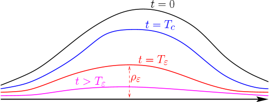
Figure 18. The two dislocations situation described in Theorem 4.

The precise result for the two dislocations collision go as follows (see Figure 18 for a sketch of this situation):

Theorem 4.

Let $N=2$ and $K=1$. Then there exist $\varepsilon_{0}>0$ and $c>0$ such that for all $\varepsilon\in(0,\varepsilon_{0})$ we have that, for all $t\geqslant T_{\varepsilon}$,

$$|v_{\varepsilon}(t,x)|\leqslant\rho_{\varepsilon}\exp\left(-\frac{c}{\varepsilon^{2s+1}}(t-T_{\varepsilon})\right),$$

where $\rho_{\varepsilon}\searrow 0$ and $T_{\varepsilon}\searrow T_{c}$ as $\varepsilon\searrow 0$.

The case of three alternate dislocations is similar, albeit different, since the steady state associated with this case is a heteroclinic and not the zero function. That is, while in the case of two dislocations the collision leads to an “annihilation to the trivial equilibrium”, in the case of three dislocations we have that two dislocations “annihilate each other”, but the third one “survives” and dictates the asymptotic behavior (see Figure 19 for a sketch of this situation). The precise result goes as follows and provides a trapping from above and below for the solution $v_{\varepsilon}$ in terms of the heteroclinic connection $u_{\star}$:

Theorem 5.

Let $N=3$, $\zeta_{1}=\zeta_{3}=1$ and $\zeta_{2}=-1$. Then there exist $\varepsilon_{0}>0$ and $c>0$ such that for all $\varepsilon\in(0,\varepsilon_{0})$ we have that, for all $t\geqslant T_{\varepsilon}$,

$$v_{\varepsilon}(t,x)\leqslant u_{\star}\left(\frac{1}{\varepsilon}\left(x-y_{\varepsilon}+\kappa_{\varepsilon}\rho_{\varepsilon}\left(1-\exp\left(-\frac{c}{\varepsilon^{2s+1}}(t-T_{\varepsilon})\right)\right)\right)\right)+\rho_{\varepsilon}\exp\left(-\frac{c}{\varepsilon^{2s+1}}(t-T_{\varepsilon})\right)$$

and

$$v_{\varepsilon}(t,x)\geqslant u_{\star}\left(\frac{1}{\varepsilon}\left(x-z_{\varepsilon}-\kappa_{\varepsilon}\rho_{\varepsilon}\left(1-\exp\left(-\frac{c}{\varepsilon^{2s+1}}(t-T_{\varepsilon})\right)\right)\right)\right)-\rho_{\varepsilon}\exp\left(-\frac{c}{\varepsilon^{2s+1}}(t-T_{\varepsilon})\right),$$

where $\rho_{\varepsilon}\searrow 0$, $\kappa_{\varepsilon}\searrow 0$, $T_{\varepsilon}\searrow T_{c}$ and $y_{\varepsilon}$, $z_{\varepsilon}\to x_{\star}$, for some $x_{\star}\in\mathbb{R}$, as $\varepsilon\searrow 0$.

In particular,

$$\limsup_{t\to+\infty}v_{\varepsilon}(t,x)\leqslant u_{\star}\left(\frac{1}{\varepsilon}\left(x-y_{\varepsilon}+\kappa_{\varepsilon}\rho_{\varepsilon}\right)\right)$$

and

$$\liminf_{t\to+\infty}v_{\varepsilon}(t,x)\geqslant u_{\star}\left(\frac{1}{\varepsilon}\left(x-z_{\varepsilon}-\kappa_{\varepsilon}\rho_{\varepsilon}\right)\right).$$

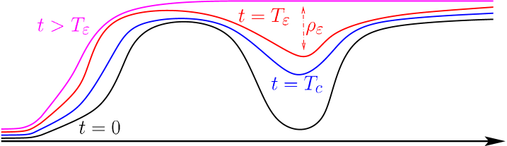
Figure 19. The three alternate dislocations situation described in Theorem 5.

The case of $N$ dislocations has been discussed in [MR3703556]. The general feature, besides technicalities, is that the parabolic character of the equation entails a “smoothing effect” on the dislocation function slightly after collision, which leads, for large time, to a precise asymptotics to either a constant function or a single heteroclinic, depending on the algebraic properties of the orientations of the initial datum.

To address the problem in its full complexity, it is convenient to distinguish the case in which the dislocations are “balanced”, i.e. $N$ is even and $K=N/2$, corresponding to the situation in which the number of positively oriented dislocation is equal to that of the negatively oriented ones, and the case in which the dislocations are “unbalanced”, namely the number of positive ones exceeds that of negative ones (or vice versa). A heuristic picture depicting the balanced case $N=4$ and $K=2$, with $\zeta_{1}=\zeta_{3}=1$ and $\zeta_{2}=\zeta_{4}=-1$ is sketched in Figure 20.

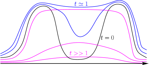
Figure 20. Time asymptotic for the balanced case.

In the balanced regime, given the normalization in (3.4), we know that, the initial dislocation function $\bar{v}_{\varepsilon}$ goes to zero both as $t\to-\infty$ and as $t\to+\infty$ and it turns out that this asymptotic behavior in space also influences the asymptotic behavior in time. More precisely, we have that after a transient time in which collisions occur, the dislocation function $v_{\varepsilon}$ relaxes to zero exponentially fast.

The unbalanced case requires a more specific analysis. In this case, we can suppose that $K<N-K$ (the case $K>N-K$ being similar) and define $\ell:=N-2K>0$. We observe that $\ell$ counts the difference between the positively oriented initial transitions (which are $N-K$) and the negatively oriented ones (which are $K$). In this case, thanks to the normalization in (3.4) the initial datum $\bar{v}_{\varepsilon}$ is asymptotic to zero as $x\to-\infty$ and to $\ell$ as $x\to+\infty$.

Given our previous discussion about the balanced case, one can expect that the long time behavior of the dislocation function is influenced by these initial conditions and one might believe that, as $t\to+\infty$ the system will try to average between the two values $0$ and $\ell$. However, this has to be taken with a pinch of salt, since the constant $\frac{\ell}{2}$ (that is the above mentioned average) is not a minimum of the potential $W$, unless $\ell$ is even, and therefore we cannot expect that $v_{\varepsilon}$ converges to $\frac{\ell}{2}$ as $t\to+\infty$, unless $\ell$ is even.

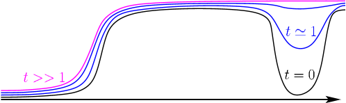
Figure 21. Time asymptotic for the unbalanced case (with $N=3$ and $K=1$).

The case $\ell$ odd needs therefore an additional analysis. On the one hand, in principle, the constant $\frac{\ell}{2}$ could be a stationary point for $W$, hence it could provide a solution of the corresponding stationary equation in (1.5). On the other hand, even if this happened, the corresponding solution would be unstable from the variational point of view, hence not suited to attract the dynamics of the parabolic flow.

As a result, when $\ell$ is odd the average constant $\frac{\ell}{2}$ is not the asymptotic limit of $v_{\varepsilon}$ as $t\to+\infty$, but it does serve as average asymptotics between the values $\frac{\ell-1}{2}$ and $\frac{\ell+1}{2}$, which are now integer and correspond to stable solutions of (1.5) induced by the minima of the potential $W$. What happens when $\ell$ is odd is thus that, as $t\to+\infty$, the dislocation function $v_{\varepsilon}$ converges to a transition layer from $\frac{\ell-1}{2}$ to $\frac{\ell+1}{2}$.

For instance, a sketch of the situation in which $N=3$ and $K=1$, with $\zeta_{1}=\zeta_{3}=1$ and $\zeta_{2}=-1$ is given in Figure 21. In this case, we have that $\ell=3-2=1$ hence $\ell$ is odd and the limit configuration in time is a transition from $\frac{\ell-1}{2}=0$ to $\frac{\ell+1}{2}=1$.

Instead, a sketch of the situation in which $N=4$ and $K=1$, with $\zeta_{1}=\zeta_{2}=\zeta_{3}=1$ and $\zeta_{4}=-1$ is given in Figure 21. In this case, we have that $\ell=4-2=2$, which is even and the asymptotic state corresponds to the constant $\frac{\ell}{2}=1$. This asymptotics is indeed reached, roughly speaking, after the collision (and consequent relaxation) of the third and forth dislocation, followed by the repulsive interaction between the first and second dislocation (this repulsion is responsible for the drift towards $-\infty$ and $+\infty$ of these two transition layers).

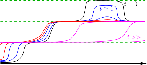
Figure 22. Time asymptotic for the unbalanced case (with $N=4$ and $K=1$).

See [MR3703556] for the corresponding formal statements. We stress that the pictures of this paper are freehand drawn, not the outcome of a careful numerical simulation, hence their intent is only explanatory, they are at best qualitative and no attempt has been made to reproduce quantitatively in the pictures the different scales involved in the asymptotics.

6. Orowan’s Law

In this section we will focus on the physical case $s=\frac{1}{2}$ and we will deduce the so-called Orowan’s Law, stating that the plastic strain velocity is proportional to the product of the density of dislocations by the effective stress.

In Section 3 we have seen that the dynamics of $N$ parallel straight dislocation lines, all lying in the same slip plane, and all positive oriented ($\xi_{i}=1$ for $i=1,\ldots,N$) can be described by the ODE’s system

(6.1) $$\begin{cases}\dot{x}_{i}(t)=\displaystyle\gamma\,\sum_{{1\leqslant j\leqslant N}\atop{j\neq i}}\frac{1}{x_{i}-x_{j}},\\ x_{i}(0)=\bar{x}_{i},\end{cases}$$

recall (3.6) and (3.7).

Here $T_{c}=+\infty$ as points with same orientation repeal each other, thus never collide. In this setting, we are interested in the case when the number $N$ of dislocation points goes to infinity. We will present below some results proven in [MR4138381] and aiming at identifying at large scale an evolution model for the dynamics of a density of dislocations. For this, let us introduce a new parameter $\delta=\delta_{\varepsilon}$ such that $\delta\to 0$ as $\varepsilon\to 0$ and let us consider the solution $v_{\varepsilon}$ of (3.3) with initial condition (3.4) (with $s=\frac{1}{2}$ and $\xi_{i}=1$), where now

$$N=N_{\delta}\sim\frac{1}{\delta}\to+\infty\quad\text{as }\varepsilon\to 0.$$

We next consider the following rescaling

$$u_{\varepsilon}(t,x):=\delta v_{\varepsilon}\left(\frac{t}{\delta},\frac{x}{\delta}\right).$$

Then $u_{\varepsilon}$ is solution to

(6.2) $$\varepsilon\partial_{t}u_{\varepsilon}=-(-\Delta)^{\frac{1}{2}}u_{\varepsilon}-\frac{1}{\varepsilon}W^{\prime}\left(\frac{u_{\varepsilon}}{\delta}\right)\quad{\mbox{ in }}\,(0,+\infty)\times\mathbb{R}$$

with initial condition

(6.3) $$u_{\varepsilon}(0,x)=\sum_{i=1}^{N_{\delta}}\delta u_{\star}\left(\frac{x-\bar{y}_{i}}{\varepsilon\delta}\right)\quad\text{on }\mathbb{R},$$

where, for $i=1,\ldots,N_{\delta}$,

$$\bar{y}_{i}:=\delta\bar{x}_{i}$$

and $u_{\star}$ is the transition layer introduced in (2.2).

Notice that with this rescaling $u_{\varepsilon}(0,x)$ (and thus, by comparison principle, $u_{\varepsilon}(t,x)$) is bounded uniformly in $\varepsilon$ as $|u_{\varepsilon}(0,x)|\leqslant N_{\delta}\delta\sim 1$.

The initial condition (6.3) can be replaced, in further generality, by any non-decreasing $C^{1,1}$ function $u_{0}$. On the other hand, any function $v\in C^{1,1}(\mathbb{R})$ which is non-decreasing and such that $v(-\infty)=0$, can be approximated by a function of the form (6.3). Indeed, given such a $v$, for $0<\delta<1$, define the $\delta i$ level set points $y_{i}$ as follows

(6.4) $$y_{i}:=\inf\{x\in\mathbb{R}\,{\mbox{ s.t. }}\,v(x)=\delta i\}\quad{\mbox{ for all }}i=1,\ldots,N_{\delta},$$

where

$$N_{\delta}:=\left\lfloor\frac{v(+\infty)-\delta}{\delta}\right\rfloor.$$

Since the function $v$ is non-decreasing, we have that $y_{i}<y_{i+1}$. Then, $v$ can be approximated in $L^{\infty}(\mathbb{R})$ as stated in the following result.

Proposition 6.

Let $v\in C^{1,1}(\mathbb{R})$ be non-decreasing, non-constant and such that $v(-\infty)=0$. Let $y_{i}$ be defined as in (6.4). Then, for all $x\in\mathbb{R}$,

$$\left|\sum_{i=1}^{N_{\delta}}\delta u_{\star}\left(\frac{x-y_{i}}{\varepsilon\delta}\right)-v(x)\right|\leqslant o_{\varepsilon,\delta}(1),$$

where $o_{\varepsilon,\delta}$ is independent of $x$ and $o_{\varepsilon,\delta}(1)\to 0$ as $\varepsilon,\delta\to 0$.

Moreover, for $v$ and $y_{i}$ as above, the following approximation formula holds true: for any $i=1,\ldots,N_{\delta}$,

(6.5) $$(-\Delta)^{\frac{1}{2}}v(y_{i})=\sum_{j\neq i}\frac{\delta}{y_{i}-y_{j}}+o_{\delta}(1),$$

where $o_{\delta}(1)\to 0$ as $\delta\to 0$, uniformly on $\mathbb{R}$. Below is the main result in this setting.

Theorem 7.

Assume that $u_{0}\in C^{1,1}(\mathbb{R})$ and $u_{0}$ is non-decreasing. Let $u_{\varepsilon}$ be the viscosity solution of (6.2), with initial condition $u_{\varepsilon}(0,x)=u_{0}(x)$, for all $x\in\mathbb{R}$. Then, as $\varepsilon\to 0$, $u_{\varepsilon}$ converges locally uniformly in $(0,+\infty)\times\mathbb{R}$ to the unique non-decreasing in $x$ viscosity solution $\bar{u}$ of

(6.6) $$\begin{cases}\partial_{t}u=-\gamma\partial_{x}u(-\Delta)^{\frac{1}{2}}u&\text{in }(0,+\infty)\times\mathbb{R},\\ u(0,\cdot)=u_{0}&\text{on }\mathbb{R},\end{cases}$$

where $\gamma$ is as in (3.7)

The limit problem (6.6) represents the plastic flow rule for the macroscopic crystal plasticity with density of dislocations, where the solution $\bar{u}$ can be interpreted as the plastic strain, $(-\Delta)^{\frac{1}{2}}\bar{u}$ is the internal stress created by the density of dislocations contained in a slip plane and identified by $\partial_{x}\bar{u}\geqslant 0$. Theorem 7 says that, in this regime, the plastic strain velocity is proportional to the dislocation density times the effective stress. This physical law is known as Orowan’s equation, see e.g. page 3739 in [sed].

Equation

(6.7) $$\partial_{t}\bar{u}=-\gamma\partial_{x}\bar{u}(-\Delta)^{\frac{1}{2}}\bar{u}$$

is an integrated form of a model studied by Head [Head] for the self-dynamics of the dislocation density $\partial_{x}\bar{u}$. Indeed, denoting by $f:=\partial_{x}\bar{u}$, differentiating (6.7), we see that, at least formally, $f$ solves

(6.8) $$\partial_{t}f=c_{0}\partial_{x}(f\mathcal{H}[f])$$

where $\mathcal{H}$is the Hilbert transform defined by

$$\mathcal{H}[f](x):=PV\int_{\mathbb{R}}\frac{f(y)}{y-x}dy.$$

Here we used that if $\bar{u}\in C^{1,\alpha}(\mathbb{R})$ and $f=\partial_{x}\bar{u}\in L^{p}(\mathbb{R})$ with $1<p<+\infty$, then an integration by parts yields

$$-(-\Delta)^{\frac{1}{2}}\bar{u}=\mathcal{H}[f].$$

The conservation of mass satisfied by the positive integrable solutions of (6.8) reflects the fact that if $f=\partial_{x}\bar{u}$ is the density of dislocations, no dislocations are created or annihilated.

Equation (6.8), called by Head the “equation of motion of the dislocation continuum”, was obtained by assuming that the speed of each dislocation is proportional to the effective stress at the dislocation.

This physical property is encoded in the limit problem (6.6). To see this, we first observe that the dislocation points can be approximated by the level set points of the limit function $\bar{u}$. More precisely, define $y_{i}(t)$ as the $\delta i$-level set of $\bar{u}(t,\cdot)$ as in (6.4). Assuming that $\bar{u}$ is smooth and $\partial_{x}\bar{u}(t,y_{i}(t))>0$, we see by differentiating in time the equation $\bar{u}(t,y_{i}(t))=\delta i$ and using (6.5) and (6.6), that

(6.9) $$\dot{y}_{i}=-\frac{\partial_{t}\bar{u}(t,y_{i}(t))}{\partial_{x}\bar{u}(t,y_{i}(t))}=\gamma(-\Delta)^{\frac{1}{2}}\bar{u}(t,y_{i}(t))\simeq\gamma\sum_{j\neq i}\frac{\delta}{y_{i}-y_{j}}.$$

Scaling back to $x_{i}(t):=y_{i}(\delta t)/\delta$, we get

$$\dot{x}_{i}\simeq\gamma\sum_{j\neq i}\frac{1}{x_{i}-x_{j}},$$

which is, up to small errors, (6.1). Moreover, from (6.9), we see that the mean velocity of each dislocation is proportional to the effective stress $(-\Delta)^{\frac{1}{2}}\bar{u}$ at the dislocation, as assumed by Head.

One can also take into account the case where dislocation points can be either positive or negative oriented, by removing the assumption that the initial datum $u_{0}$ is non-decreasing. In this situation Theorem 7 is generalized in a forthcoming paper [pnespre] as follows.

Theorem 8.

Assume that $u_{0}\in C^{1,1}(\mathbb{R})$ and that the limits $u(+\infty)$ and $u(-\infty)$ exist. Let $u_{\varepsilon}$ be the viscosity solution of (6.2), with initial condition $u_{\varepsilon}(0,x)=u_{0}(x)$, for all $x\in\mathbb{R}$. Then, as $\varepsilon\to 0$, $u_{\varepsilon}$ converges locally uniformly in $(0,+\infty)\times\mathbb{R}$ to the viscosity solution $\bar{u}$ of

(6.10) $$\begin{cases}\partial_{t}u=-\gamma|\partial_{x}u|(-\Delta)^{\frac{1}{2}}u&\text{in }(0,+\infty)\times\mathbb{R},\\ u(0,\cdot)=u_{0}&\text{on }\mathbb{R},\end{cases}$$

where $\gamma$ is as in (3.7).

Differentiating equation $\partial_{t}\bar{u}=-\gamma|\partial_{x}\bar{u}|(-\Delta)^{\frac{1}{2}}\bar{u}$ yields the two following equations for the positive and negative part of $f=\partial_{x}\bar{u}$,

$$\partial_{t}f^{+}=\partial_{x}(f^{+}\mathcal{H}(f^{+}-f^{-})),\quad\partial_{t}f^{-}=-\partial_{x}(f^{-}\mathcal{H}(f^{+}-f^{-}))$$

which are the 1-D version of the 2-D Groma-Balogh equations [groma], a macroscopic model describing the evolution of the density of positive and negative oriented parallel straight dislocation lines. In this model in which collisions may occur, the mass of the dislocation density $|\partial_{x}\bar{u}|=f^{+}+f^{-}$ is not in general preserved, while it is preserved the mass of $f^{+}-f^{-}$, more precisely: for all $t>0$, $\bar{u}(t,+\infty)=u_{0}(+\infty)$ and $\bar{u}(t,-\infty)=u_{0}(-\infty)$, as shown in [pnespre].

7. Homogenization

In this section, we consider equation (6.2) in any dimensions $n\geqslant 1$ and we deal with the corresponding homogenization problem.

To this end, we recall that the parameter $\varepsilon$ in (6.2) describes the ratio between the microscopic and the mesoscopic scale, where the discrete dynamics of dislocations is given by the ODE system (3.6). Thus, recalling the initial condition (3.4), the parameter $\varepsilon$ can also be interpreted as the distance between dislocation points at microscopic scale.

In this section, we freeze $\varepsilon$, namely we keep this distance fixed but, as in Section 6, we let the number of dislocation points go to infinity. Hence, without loss of generality, we can assume $\varepsilon=1$. Thus we deal with the problem

(7.1) $$\begin{cases}\partial_{t}u_{\delta}=-(-\Delta)^{\frac{1}{2}}u_{\delta}-W^{\prime}\left(\displaystyle\frac{u_{\delta}}{\delta}\right)&{\mbox{ in }}\,(0,+\infty)\times\mathbb{R}^{n},\\ u_{\delta}(0,x)=u_{0}(x)&\text{ on }\mathbb{R}^{n}.\end{cases}$$

The case $n>1$, in particular $n=2$, allows us to consider dislocation lines, all lying in the same slip plane, which can be curved and thus for which the reduction of dimension argument described in the introduction cannot be applied.

One could also eventually add on the right hand-side of the PDE in (7.1) a term of the form $\sigma(t/\delta,x/\delta)$, where $\sigma$ is periodic in both $t$ and $x$, representing a stress created by the obstacles in the crystal or/and an applied exterior stress. For simplicity of presentation, as before we will take $\sigma\equiv 0$.

The behavior of the solution $u_{\delta}$ of (7.1) has been investigated in [monpatr1]. From a mathematical viewpoint, problem (7.1) is a homogenization problem, and as usual in periodic homogenization (recall that the potential $W$ is periodic), the limit equation is determined by a cell problem. In this case, such a problem is, for any $p\in\mathbb{R}^{n}$ and $L\in\mathbb{R}$, the following

(7.2) $$\begin{cases}\partial_{\tau}w=-(-\Delta)^{\frac{1}{2}}w+L-W^{\prime}(w+p\cdot y)&\text{in}\quad(0,+\infty)\times\mathbb{R}^{n},\\ w(0,y)=0&\text{on}\quad\mathbb{R}^{n},\end{cases}$$

and one looks for some $\lambda\in\mathbb{R}$ for which $w-\lambda\tau$ is bounded. The precise result goes as follows.

Theorem 9.

For $L\in\mathbb{R}$ and $p\in\mathbb{R}^{n}$, there exists a unique viscosity solution $w\in C((0,+\infty)\times\mathbb{R}^{n})$ of (7.2) and there exists a unique $\lambda\in\mathbb{R}$ such that $w$ satisfies

$$\frac{w(\tau,y)}{\tau} \lambda \tau\rightarrow+\infty y$$ converges towards as , locally uniformly in .

The real number $\lambda$ is denoted by $\overline{H}(p,L)$. The function $\overline{H}(p,L)$ is continuous on $\mathbb{R}^{n}\times\mathbb{R}$ and non-decreasing in $L$.

The function $\overline{H}(p,L)$ defined through the cell-problem (7.2) is called effective Hamiltonian, and the homogenized limit problem is given by

(7.3) $$\begin{cases}\partial_{t}u=\overline{H}(\nabla_{x}u,-(-\Delta)^{\frac{1}{2}}u)&\text{in}\quad(0,+\infty)\times\mathbb{R}^{n},\\ u(0,x)=u_{0}(x)&\text{on}\quad\mathbb{R}^{n},\end{cases}$$

as stated below.

Theorem 10.

The solution $u_{\delta}$ of (7.1) converges towards the unique viscosity solution $u^{0}$ of (7.3) locally uniformly in $(t,x)$, as $\delta\searrow 0$, where $\overline{H}$ is defined in Theorem 9.

As for the limit problems (6.6) and (6.10), the function $u^{0}$ can be interpreted as a macroscopic plastic strain satisfying the macroscopic plastic flow rule (7.3). Moreover $(-\Delta)^{\frac{1}{2}}u^{0}$ is the stress created by the macroscopic density of dislocations, $\nabla u^{0}$ is the vectorial dislocation density and $|\nabla u^{0}|$ is the scalar dislocation density.

The behavior of $\overline{H}(p,L)$ for small stress $L$ and small density $|p|$, in dimension $n=1$, has been investigated in [monpatr2]. In this regime is it shown that

(7.4) $$\overline{H}(p,L)\simeq\gamma|p|L,$$

thus recovering again the Orowan’s Law discussed in Section 6. More precisely:

Theorem 11.

Let $p_{0},\,L_{0}\in\mathbb{R}$. Then the function $\overline{H}$ defined in Theorem 9 satisfies

$$\frac{\overline{H}(\varepsilon p_{0},\varepsilon L_{0})}{\varepsilon^{2}}\rightarrow\gamma|p_{0}|L_{0}\quad\text{as }\varepsilon\rightarrow 0^{+},$$

where $\gamma$ is as in (3.7).

When the exterior force $\sigma$ does not vanish identically but has zero mean value, it is expected, but not proven, a threshold phenomenon as in [imr], that is

$$\overline{H}(p,L)=0\quad\mbox{if}\quad|L|\quad\mbox{is small enough}.$$

This means more generally that this homogenization procedure describes correctly the mechanical behaviour of the stress at large scales, but keeps the memory of the microstructure in the plastic law with possible threshold effects.

The results contained in Theorems 10 and 11 have been generalized in [MR3334171] to the case where $(-\Delta)^{\frac{1}{2}}$ is replaced by $(-\Delta)^{s}$ with $s\in(0,1)$. The scaling of the system and the results obtained are different according to the fractional parameter $s\in(0,1)$. Namely, when $s>1/2$ the effective Hamiltonian “localizes” and it only depends on a first order differential operator. Instead, when $s<1/2$, the non-local features are predominant and the effective Hamiltonian involves the fractional operator of order $s$. That is, roughly speaking, for any $s\in(0,1)$, the effective Hamiltonian is an operator of order $\min\{2s,1\}$, which reveals the stronger non-local effects present in the case $s<1/2$.

The homogenization problems become

(7.5) $$\begin{cases}\partial_{t}u_{\delta}=-\delta^{2s-1}(-\Delta)^{s}u_{\delta}-W^{\prime}\left(\frac{u_{\delta}}{\delta}\right)&\text{in}\quad(0,+\infty)\times\mathbb{R}^{n},\\ u_{\delta}(0,x)=u_{0}(x)&\text{on}\quad\mathbb{R}^{n},\end{cases}$$

for $s>\frac{1}{2}$, and

(7.6) $$\begin{cases}\partial_{t}u_{\delta}=-(-\Delta)^{s}u_{\delta}-W^{\prime}\left(\frac{u_{\delta}}{\delta^{2s}}\right)+&\text{in}\quad(0,+\infty)\times\mathbb{R}^{n},\\ u_{\delta}(0,x)=u_{0}(x)&\text{on}\quad\mathbb{R}^{n},\end{cases}$$

for $s<\frac{1}{2}$.

Notice that the two different scalings formally coincide when $s=\frac{1}{2}$. The solution $u_{\delta}$ of (7.5) converges as $\delta\rightarrow 0$ to the solution $u^{0}$ of the homogenized problem

(7.7) $$\begin{cases}\partial_{t}u=\overline{H}_{1}(\nabla_{x}u)&\text{in}\quad(0,+\infty)\times\mathbb{R}^{n},\\ u(0,x)=u_{0}(x)&\text{on}\quad\mathbb{R}^{n},\end{cases}$$

with an effective Hamiltonian $\overline{H}_{1}$ which does not depend on the fractional Laplacian anymore, while the solution $u_{\delta}$ of (7.6) converges as $\delta\searrow 0$ to $u^{0}$ solution of the following problem

(7.8) $$\begin{cases}\partial_{t}u=\overline{H}_{2}(-(-\Delta)^{s}u)&\text{in}\quad(0,+\infty)\times\mathbb{R}^{n},\\ u(0,x)=u_{0}(x)&\text{on}\quad\mathbb{R}^{n},\end{cases}$$

with an effective Hamiltonian $\overline{H}_{2}$ not depending on the gradient.

The functions $\overline{H}_{1}$ and $\overline{H}_{2}$ are determined by the following cell problem: for $p\in\mathbb{R}^{n}$ and $L\in\mathbb{R}$,

(7.9) $$\begin{cases}\partial_{\tau}w=-(-\Delta)^{s}w+L-W^{\prime}(w+p\cdot y)&\text{in}\quad(0,+\infty)\times\mathbb{R}^{n},\\ w(0,y)=0&\text{on}\quad\mathbb{R}^{n},\end{cases}$$

that is $\overline{H}_{1}$ and $\overline{H}_{2}$ are determined by the unique $\lambda$ for which $w-\lambda\tau$ is bounded (according to the cases $s>\frac{1}{2}$ and $s<\frac{1}{2}$, respectively). More precisely, as before we have:

Theorem 12.

For $L\in\mathbb{R}$ and $p\in\mathbb{R}^{n}$, there exists a unique viscosity solution $w\in C((0,+\infty)\times\mathbb{R}^{n})$ of (7.9) and there exists a unique $\lambda\in\mathbb{R}$ such that $w$ satisfies:

$$\frac{w(\tau,y)}{\tau} \lambda \tau\rightarrow+\infty y$$ converges towards as , locally uniformly in .

The real number $\lambda$ is denoted by $\overline{H}(p,L)$. The function $\overline{H}(p,L)$ is continuous on $\mathbb{R}^{n}\times\mathbb{R}$ and non-decreasing in $L$.

Once the cell problem is solved, the convergence results go as follows:

Theorem 13.

The solution $u_{\delta}$ of (7.5) converges towards the solution $u^{0}$ of (7.7) locally uniformly in $(t,x)$ as $\delta\searrow 0$, where

$$\overline{H}_{1}(p):=\overline{H}(p,0)$$

and $\overline{H}(p,L)$ is defined in Theorem 12.

Theorem 14.

The solution $u_{\delta}$ of (7.6) converges towards the solution $u^{0}$ of (7.8) locally uniformly in $(t,x)$ as $\delta\searrow 0$, where

$$\overline{H}_{2}(L):=\overline{H}(0,L)$$

and $\overline{H}(p,L)$ is defined in Theorem 12.

The following extension of the Orowan’s Law is also proven in [MR3334171].

Theorem 15.

Let $p_{0},\,L_{0}\in\mathbb{R}$ with $p_{0}\neq 0$. Then the function $\overline{H}$ defined in Theorem 12 satisfies

$$\frac{\overline{H}(\delta p_{0},\varepsilon^{2s}L_{0})}{\varepsilon^{1+2s}}\rightarrow\gamma|p_{0}|L_{0}\quad\text{as }\varepsilon\rightarrow 0^{+},$$

where $\gamma$ is as in (3.7).