A Hong-Krahn-Szegö inequality
for mixed local and nonlocal operators

Abstract.

Given a bounded open set $\Omega\subseteq\mathbb{R}^{n}$, we consider the eigenvalue problem of a nonlinear mixed local/nonlocal operator with vanishing conditions in the complement of $\Omega$.

We prove that the second eigenvalue $\lambda_{2}(\Omega)$ is always strictly larger than the first eigenvalue $\lambda_{1}(B)$ of a ball $B$ with volume half of that of $\Omega$.

This bound is proven to be sharp, by comparing to the limit case in which $\Omega$ consists of two equal balls far from each other. More precisely, differently from the local case, an optimal shape for the second eigenvalue problem does not exist, but a minimizing sequence is given by the union of two disjoint balls of half volume whose mutual distance tends to infinity.

1. Introduction

In this paper we consider a nonlinear operator arising from the superposition of a classical $p$-Laplace operator and a fractional $p$-Laplace operator, of the form

(1.1) $$\mathcal{L}_{p,s}=-\Delta_{p}+(-\Delta)^{s}_{p}$$

with $s\in(0,1)$ and $p\in[2,+\infty)$. Here the fractional $p$-Laplace operator is defined, up to a multiplicative constant that we neglect, as

$$(-\Delta)^{s}_{p}u(x):=2\int_{\mathbb{R}^{n}}\frac{|u(x)-u(y)|^{p-2}(u(x)-u(y))}{|x-y|^{n+ps}}\,dy.$$

Given a bounded open set $\Omega\subseteq\mathbb{R}^{n}$, we consider the eigenvalue problem for the operator $\mathcal{L}_{p,s}$ with homogeneous Dirichlet boundary conditions (i.e., the eigenfunctions are prescribed to vanish in the complement of $\Omega$). In particular, we define $\lambda_{1}(\Omega)$ to be the smallest of such eigenvalues and $\lambda_{2}(\Omega)$ to be the second smallest one (in the sense made precise in [9, 41]).

The main result that we present here is a version of the Hong–Krahn–Szegö inequality for the second Dirichlet eigenvalue $\lambda_{2}(\Omega)$, according to the following statement:

Theorem 1.1.

Let $\Omega\subseteq\mathbb{R}^{n}$ be a bounded open set. Let $B$ be any Euclidean ball with volume $|\Omega|/2$. Then,

(1.2) $$\lambda_{2}(\Omega)>\lambda_{1}(B).$$

Furthermore, equality is never attained in (1.2); however, the estimate is sharp in the following sense: if $\{x_{j}\}_{j},\,\{y_{j}\}_{j}\subseteq\mathbb{R}^{n}$ are two sequences such that

$$\lim_{j\to+\infty}|x_{j}-y_{j}|=+\infty,$$

and if we define $\Omega_{j}:=B_{r}(x_{j})\cup B_{r}(y_{j})$, then

(1.3) $$\lim_{j\to+\infty}\lambda_{2}(\Omega_{j})=\lambda_{1}(B_{r}).$$

To the best of our knowledge, Theorem 1.1 is new even in the linear case $p=2$. Also, an interesting consequence of the fact that equality in (1.2) is never attained is that, for all $c>0$, the shape optimization problem

$$\inf_{|\Omega|=c}\lambda_{2}(\Omega)$$

does not admit a solution.

Before diving into the technicalities of the proof of Theorem 1.1, we recall in the forthcoming Section 1.1 some classical motivations to study first and second eigenvalue problems, then we devote Section 1.2 to showcase the available results on the shape optimization problems related to the first and the second eigenvalues of several elliptic operators.

1.1. The importance of the first and second eigenvalues

The notion of eigenvalue seems to date back to the 18th century, due to the works of Euler and Lagrange on rigid bodies. Possibly inspired by Helmholtz, in his study of integral operators [43] Hilbert introduced the terminology of “Eigenfunktion” and “Eigenwert” from which the modern terminology of “eigenfunction” and “eigenvalue” originated.

The analysis of eigenvalues also became topical in quantum mechanics, being equivalent in this setting to the energy of a quantum state of a system, and in general in the study of wave phenomena, to distinguish high and low frequency components.

In modern technologies, a deep understanding of eigenvalues has become a central theme of research, especially due to the several ranking algorithms, such as PageRank (used by search engines as Google to rank the results) and EigenTrust (used by peer-to-peer networks to establish a trust value on the account of authentic and corrupted resources). In a nutshell, these algorithms typically have entries (e.g. the page rank of a given website, or the trust value of a peer) that are measured as linear superpositions of the other entries. For instance (see Section 2.1.1 in [17], neglecting for simplicity damping factors) one can model the page rank $p_{i}$ of website $i$ in terms of the ratio $R_{ij}$ between the number of links outbound from website $j$ to page $i$ and the total number of outbound links of website $j$, namely

(1.4) $$p_{i}=\sum_{j}R_{ij}p_{j}.$$

Whether this is a finite or infinite sum boils down to a merely philosophical question, given the huge number of websites explored by Google, but let us stick for the moment with the discrete case of finitely many websites. Interestingly $p_{i}$ basically counts the probability that a random surfer visits website $i$ by following the available links in the web.

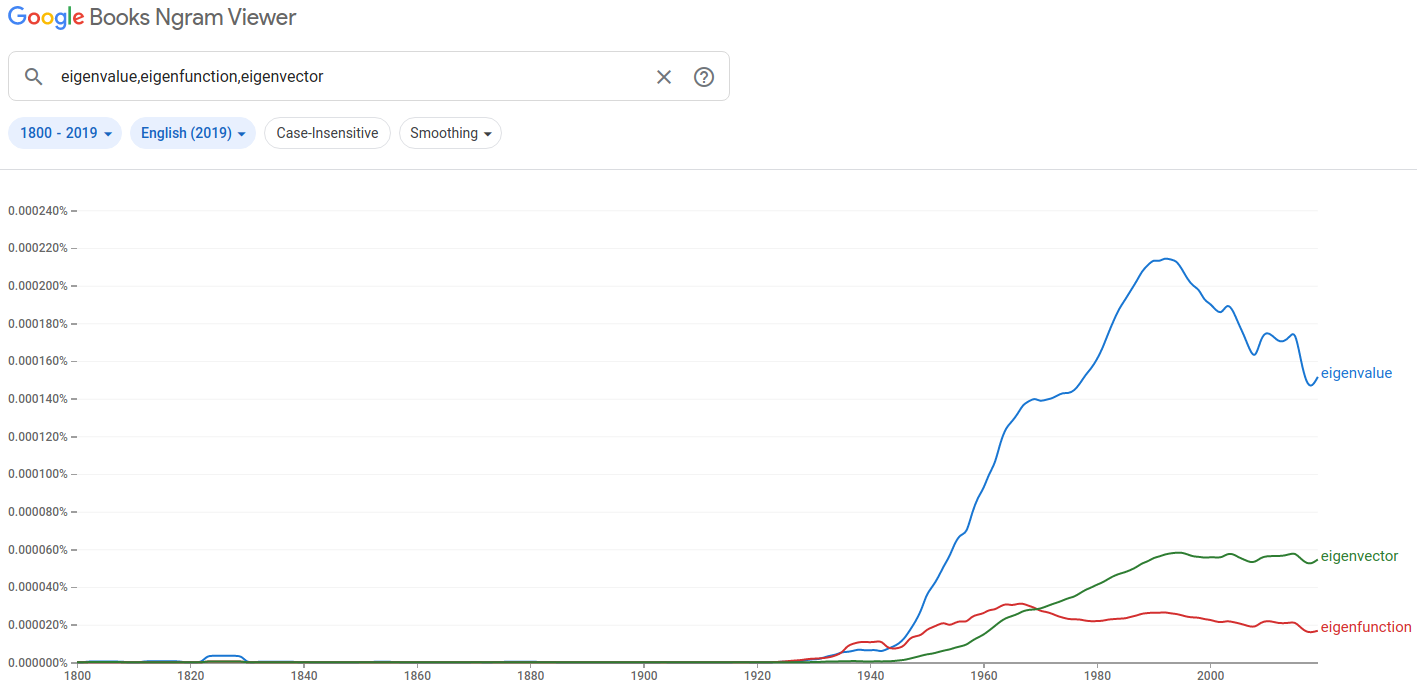
Figure 1.

Now, in operator form, one can write (1.4) as $p=Rp$, with the matrix $R$ known in principle from the outbound links of the websites and the ranking array $p$ to be determined. Thus, up to diagonalizing $R$, the determination of $p$ reduces to the determination of the eigenvectors of $R$, or equivalently to the determination of the eigenvectors of the inverse matrix $A:=R^{-1}$, and this task can be accomplished, for instance, by iterative algorithms.

The simplest of these algorithms used in PageRank is probably the power iteration method. For instance, if one defines $\eta_{k+1}:=\frac{A\eta_{k}}{|A\eta_{k}|}$, given a random starting vector $\eta_{0}$, it follows that $\eta_{k}=\frac{A^{k}\eta_{0}}{|A^{k}\eta_{0}|}$ and consequently, if $\eta_{0}=\sum_{j}c_{j}w_{j}$, being $w_{j}$ the eigenvectors of $A$ with corresponding eigenvalues $\mu_{1}>\mu_{2}\geq\mu_{3}\geq...$ (normalized to have unit length), we find that

$$\eta_{k}=\frac{\sum_{j}c_{j}\mu_{j}^{k}w_{j}}{\left|\sum_{j}c_{j}\mu_{j}^{k}w_{j}\right|}=\frac{\sum_{j}d_{jk}w_{j}}{\left|\sum_{j}d_{jk}w_{j}\right|}=\frac{w_{1}+\sum_{j\neq 1}d_{jk}w_{j}}{\left|{\rm{sign}}(c_{1})w_{1}+\sum_{j\neq 1}d_{jk}w_{j}\right|}.$$

with $d_{jk}:=\frac{c_{j}\mu_{j}^{k}}{c_{1}\mu_{1}^{k}}$ (here we are assuming that the eigenvalues are positive and that, in view of the randomness of $\eta_{0}$, we have that $c_{1}\neq 0$).

Since

$$\left|\sum_{j\neq 1}d_{jk}w_{j}\right|^{2}=\sum_{j\neq 1}d_{jk}^{2}=\sum_{j\neq 1}\frac{c_{j}^{2}\mu_{j}^{2k}}{c_{1}^{2}\mu_{1}^{2k}}=O\left(\frac{\mu_{2}^{2k}}{\mu_{1}^{2k}}\right),$$

it follows that

$$\eta_{k}=w_{1}+O\left(\frac{\mu_{2}^{k}}{\mu_{1}^{k}}\right)$$

and accordingly $\eta_{k}$ approximates the eigenfunction $w_{1}$ with a convergence induced by the ratio $\frac{\mu_{2}}{\mu_{1}}<1$.

That is, if $\lambda_{1}<\lambda_{2}\leq\lambda_{3}\leq\dots$ are the eigenvalues of the matrix $R$, the above rate of convergence is dictated by the ratio $\frac{\lambda_{1}}{\lambda_{2}}$ of the smallest and second smallest eigenvalues of $R$. This is one simple, but, in our opinion quite convincing, example of the importance of the first two eigenvalues in problems with concrete applications.

To confirm the importance of the notion of eigenvalues in the modern technologies, see Figure 1 for a Google Ngram Viewer charting the frequencies of use of the words eigenvalue, eigenfunction and eigenvector in the last 120 years.

Also, to highlight the importance of the difference between the first and second eigenvalues, see Figure 2 for a Google Ngram Viewer charting the frequencies of use of the words eigengap and spectral gap in the last 120 years.

In the case of the Google PageRank, an efficient estimate of the eigengap taking into account the damping factor has been proposed in [42].

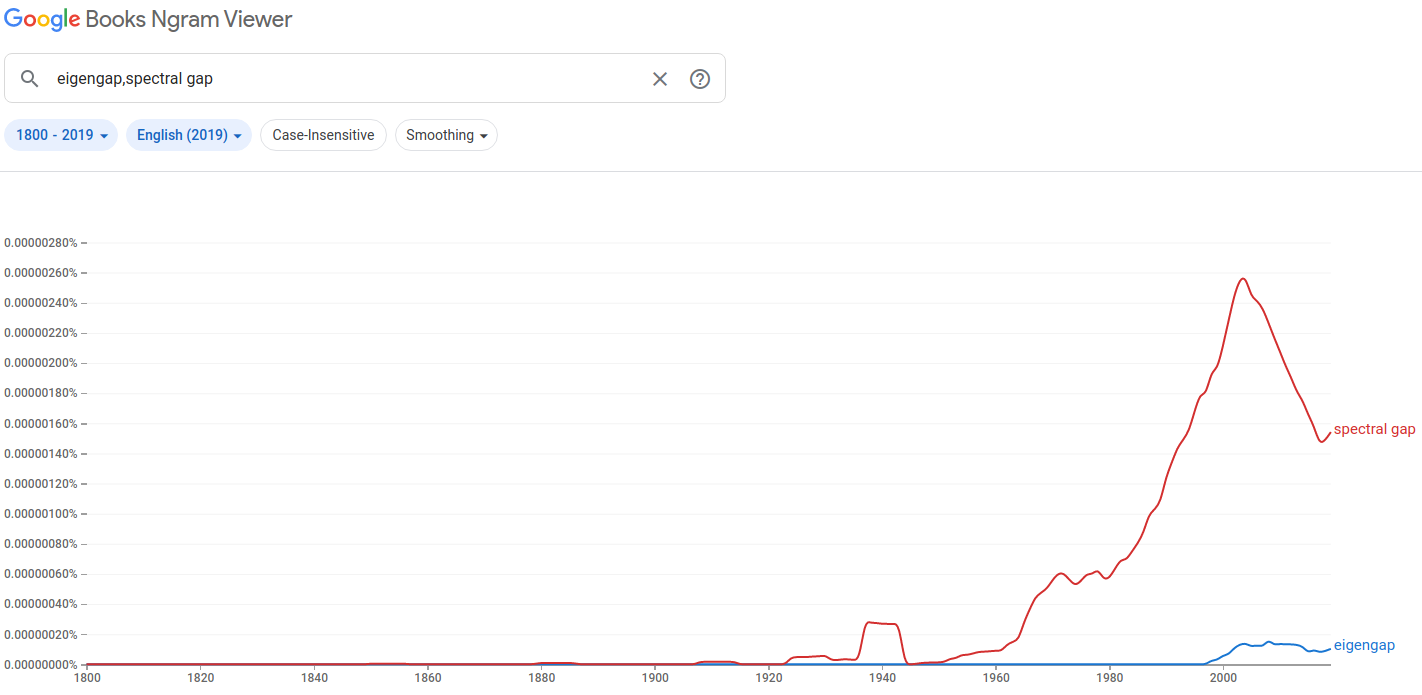
Figure 2.

1.2. Shape optimization problems for the first and second eigenvalues in the context of elliptic (linear and nonlinear, classical and fractional) equations

Now we leave the realm of high-tech applications and we come back to the partial differential equations and fractional equations setting: in this framework, we recall here below some of the main results about shape optimization problems related to the first and the second eigenvalues.

1.2.1. The case of the Laplacian

One of the classical shape optimization problem is related to the detection of the domain that minimizes the first eigenvalue of the Laplacian with homogeneous boundary conditions. This is the content of the Faber–Krahn inequality [31, 47], whose result can be stated by saying that among all domains of fixed volume, the ball has the smallest first eigenvalue.

In particular, as a physical application, one has that that among all drums of equal area, the circular drum possesses the lowest voice, and this somewhat corresponds to our intuition, since a very elongated rectangular drum produces a high pitch related to the oscillations along the short edge.

Another physical consequence of the Faber–Krahn inequality is that among all the regions of a given volume with the boundary maintained at a constant temperature, the one which dissipates heat at the slowest possible rate is the sphere, and this also corresponds to our everyday life experience of spheres minimizing contact with the external environment thus providing the optimal possible insulation.

From the mathematical point of view, the Faber–Krahn inequality also offers a classical stage for rearrangement methods and variational characterizations of eigenvalues.

In view of the discussion in Section 1.1, the subsequent natural question investigates the optimal shape of the second eigenvalue. This problem is addressed by the Hong–Krahn–Szegö inequality [48, 44, 52], which asserts that among all domains of fixed volume, the disjoint union of two equal balls has the smallest second eigenvalue.

Therefore, for the case of the Laplacian with homogeneous Dirichlet data, the shape optimization problems related to both the first and the second eigenvalues are solvable and the solution has a simple geometry.

It is also interesting to point out a conceptual connection between the Faber–Krahn and the Hong–Krahn–Szegö inequalities, in the sense that the proof of the second typically uses the first one as a basic ingredient. More specifically, the strategy to prove the Hong–Krahn–Szegö inequality is usually:

• Use that in a connected open set all eigenfunctions except the first one must change sign,

• Deduce that $\lambda_{2}(\Omega)=\max\{\lambda_{1}(\Omega_{+}),\lambda_{1}(\Omega_{-})\}$, for suitable subdomain $\Omega_{+}$ and $\Omega_{-}$ which are either nodal domains for the second eigenfunction, if $\Omega$ is connected, or otherwise connected components of $\Omega$,

• Utilize the Faber–Krahn inequality to show that $\lambda_{1}(\Omega_{\pm})$ is reduced if we replace $\Omega_{\pm}$ with a ball of volume $|\Omega_{\pm}|$,

• Employ the homogeneity of the problem to deduce that the volumes of these two balls are equal.

That is, roughly speaking, a cunning use of the Faber–Krahn inequality allows one to reduce to the case of disjoint balls, which can thus be addressed specifically.

1.2.2. The case of the $p$-Laplacian

A natural extension of the optimal shape results for the Laplacian recalled in Section 1.2.1 is the investigation of the nonlinear operator setting and in particular the case of the $p$-Laplacian. This line of research was carried out in [12] in which a complete analogue of the results of Section 1.2.1 have been established for the $p$-Laplacian. In particular, the first Dirichlet eigenvalue of the $p$-Laplacian is minimized by the ball and the second by any disjoint union of two equal balls.

We stress that, in spite of the similarity of the results obtained, the nonlinear case presents its own specific peculiarities. In particular, in the case of the $p$-Laplacian one can still define the first eigenvalue by minimization of a Rayleigh quotient, in principle the notion of higher eigenvalues become more tricky, since discreteness of the spectrum is not guaranteed and the eigenvalues theory for nonlinear operators offers plenty of open problems at a fundamental level. For the second eingevalue however one can obtain a variational characterization in terms of a mountain-pass result, still allowing the definition of a spectral gap between the smallest and the second smallest eigenvalue.

1.2.3. The cases of the fractional Laplacian and of the fractional $p$-Laplacian

We now consider the question posed by the minimization of the first and second eigenvalues in a nonlocal setting.

The optimal shape problems for the first eigenvalue of the fractional Laplacian with homogeneous external datum was addressed in [3, 13, 56, 11], showing that the ball is the optimizer.

As for the nonlinear case, the spectral properties of the fractional $p$-Laplacian possess their own special features, see [34], and they typically combine the difficulties coming from the nonlocal world with those arising from the theory of nonlinear operators. In [13] the optimal shape problem for the first Dirichlet eigenvalue of the fractional $p$- Laplacian was addressed, by detecting the optimality of the ball as a consequence of a general Pòlya–Szegö principle.

For the second eigenvalue, however, the situation in the nonlocal case is quite different from the classical one, since in general nonlocal energy functionals are deeply influenced by the mutual position of the different connected components of the domain, see [50].

In particular, the counterpart of the Hong–Krahn–Szegö inequality for the fractional Laplacian and the fractional $p$-Laplacian was established in [15] and it presents significant differences with the classical case: in particular, the shape optimizer for the second eigenvalue of the fractional $p$-Laplacian with homogeneous external datum does not exist and one can bound such an eigenvalue from below by the first eigenvalue of a ball with half of the volume of the given domain (and this is the best lower bound possible, since the case of a domain consisting of two equal balls drifting away from each other would attain such a bound in the limit).

1.2.4. The case of mixed operators

The study of mixed local/nonlocal operators has been recently received an increasing level of attention, both in view of their intriguing mathematical structure, which combines the classical setting and the features typical of nonlocal operators in a framework that is not scale-invariant [40, 45, 46, 5, 32, 10, 21, 4, 20, 24, 23, 22, 39, 7, 1, 18, 30, 27, 28, 35, 36, 37, 38, 19, 9, 6, 54], and of their importance in practical applications such as the animal foraging hypothesis [29, 51].

In regard to the shape optimization problem, a Faber–Krahn inequality for mixed local and nonlocal linear operators when $p=2$ has been established in [8], showing the optimality of the ball in the minimization of the first eigenvalue. The corresponding inequality for the nonlinear setting presented in (1.1) will be given here in the forthcoming Theorem 4.1.

The inequality of Hong–Krahn–Szegö type for mixed local and nonlocal linear operators presented in (1.1) would thus complete the study of the optimal shape problems for the first and second eigenvalues of the operator in (1.1).

1.3. Plan of the paper

The rest of this paper is organized as follows. Section 2 sets up the notation and collects some auxiliary results from the existing literature.

In Section 3 we discuss a regularity theory which, in our setting, plays an important role in the proof of Theorem 1.1 in allowing us to speak about nodal regions for the corresponding eigenfunction (recall the bullet point strategy presented on page • ‣ 1.2.1). In any case, this regularity theory holds in a more general setting and can well come in handy in other situations as well.

Finally, Section 4 introduces the corresponding Faber–Krahn inequality for the operator in (1.1) and completes the proof of Theorem 1.1.

2. Preliminaries

To deal with the nonlinear and mixed local/nonlocal operator in (1.1), given and open and bounded set $\Omega\subseteq\mathbb{R}^{n}$, it is convenient to introduce the space

$$\mathcal{X}_{0}^{1,p}(\Omega)\subseteq W^{1,p}(\mathbb{R}^{n}),$$

defined as the closure of $C_{0}^{\infty}(\Omega)$ with respect to the global norm

$$u\mapsto\Big{(}\int_{\mathbb{R}^{n}}|\nabla u|^{p}\,dx\Big{)}^{1/p}.$$

We highlight that, since $\Omega$ is bounded, $\mathcal{X}^{1,p}_{0}(\Omega)$ can be equivalently defined by taking the closure of $C_{0}^{\infty}(\Omega)$ with respect to the full norm

$$u\mapsto\bigg{(}\int_{\mathbb{R}^{n}}|u|^{p}\,dx\bigg{)}^{1/p}+\bigg{(}\int_{\mathbb{R}^{n}}|\nabla u|^{p}\,dx\bigg{)}^{1/p};$$

however, we stress that $\mathcal{X}_{0}^{1,p}(\Omega)$ is different from the usual space $W^{1,p}_{0}(\Omega)$, which is defined as the closure of $C_{0}^{\infty}(\Omega)$ with respect to the norm

$$u\mapsto\Big{(}\int_{\Omega}|\nabla u|^{p}\,dx\Big{)}^{1/p}.$$

As a matter of fact, while the belonging of a function $u$ to $W^{1,p}_{0}(\Omega)$ only depends on its behavior inside of $\Omega$ (actually, $u$ does not even need to be defined outside of $\Omega$), the belonging of $u$ to $\mathcal{X}_{0}^{1,p}(\Omega)$ is a global condition, and it depends on the behavior of $u$ on the whole space $\mathbb{R}^{n}$ (in particular, $u$ has to be defined on $\mathbb{R}^{n}$). Just to give an example of the difference between these spaces, let $u\in C^{\infty}_{0}(\mathbb{R}^{n})\setminus\{0\}$ be such that

$$\mathrm{supp}(u)\cap\overline{\Omega}=\varnothing.$$

Since $u\equiv 0$ inside of $\Omega$, we clearly have that $u\in W^{1,p}_{0}(\Omega)$; on the other hand, since $u\not\equiv 0$ in $\mathbb{R}^{n}\setminus\Omega$, one has $u\notin\mathcal{X}_{0}^{1,p}(\Omega)$ (even if $u\in W^{1,p}(\mathbb{R}^{n})$).

Although they do not coincide, the spaces $\mathcal{X}_{0}^{1,p}(\Omega)$ and $W^{1,p}_{0}(\Omega)$ are related: to be more precise, using [16, Proposition 9.18] and taking into account the definition of $\mathcal{X}_{0}^{1,p}(\Omega)$, one can see that

• if $u\in W_{0}^{1,p}(\Omega)$, then $u\cdot\mathbf{1}_{\Omega}\in\mathcal{X}_{0}^{1,p}(\Omega)$;

• if $u\in\mathcal{X}_{0}^{1,p}(\Omega)$, then $u\big{|}_{\Omega}\in W_{0}^{1,p}(\Omega)$.

Moreover, we can actually characterize $\mathcal{X}_{0}^{1,p}(\Omega)$ as follows:

$$\mathcal{X}_{0}^{1,p}(\Omega)=\{u\in W^{1,p}(\mathbb{R}^{n}):\,\text{$u\big{|}_{\Omega}\in W^{1,p}_{0}(\Omega)$ and $u=0$ a.e.\,in $\mathbb{R}^{n}\setminus\Omega$}\}.$$

The main issue in trying to use (i)-(ii) to identify $W_{0}^{1,p}(\Omega)$ with $\mathcal{X}_{0}^{1,p}(\Omega)$ is that, if $u$ is globally defined and $u\in W^{1,p}(\mathbb{R}^{n})$, then

$$u\big{|}_{\Omega}\in W^{1,p}_{0}(\Omega)\,\,\Rightarrow\,\,u\cdot\mathbf{1}_{\Omega}\in\mathcal{X}_{0}^{1,p}(\Omega);$$

however, we cannot say (in general) that $u\neq u\cdot\mathbf{1}_{\Omega}$. Even if they cannot allow to identify $\mathcal{X}_{0}^{1,p}(\Omega)$ with $W_{0}^{1,p}(\Omega)$, assertions (i)-(ii) can be used to deduce several properties of the space $\mathcal{X}_{0}^{1,p}(\Omega)$ starting from their analog in $W_{0}^{1,p}(\Omega)$; for example, we have the following fact, which shall be used in the what follows:

$$u\in\mathcal{X}_{0}^{1,p}(\Omega)\,\,\Rightarrow\,\,|u|,\,u^{+},\,u^{-}\in\mathcal{X}_{0}^{1,p}(\Omega).$$

Remark 2.1.

In the particular case when the open set $\Omega$ is of class $C^{1}$, it follows from [16, Proposition 9.18] that, if $u\in W^{1,p}(\mathbb{R}^{n})$ and $u=0$ a.e. in $\mathbb{R}^{n}\setminus\Omega$, then

$$u\big{|}_{\Omega}\in W_{0}^{1,p}(\Omega).$$

As a consequence, we have

$$\mathcal{X}_{0}^{1,p}(\Omega)=\{u\in W^{1,p}(\Omega):\,\text{$u=0$ a.e.\,in $\mathbb{R}^{n}\setminus\Omega$}\}.$$

This fact shows that, when $\Omega$ is sufficiently regular, $\mathcal{X}_{0}^{1,p}(\Omega)$ coincides with the space $\mathbb{X}_{p}(\Omega)$ introduced in [6] (for $p=2$) and in [9] (for a general $p>1$).

For future reference, we introduce the following set

(2.1) $$\mathcal{M}(\Omega):=\bigg{\{}u\in\mathcal{X}_{0}^{1,p}(\Omega):\,\int_{\mathbb{R}^{n}}|u|^{p}\,dx=1\bigg{\}}.$$

After these preliminaries, we can turn our attention to the Dirichlet problem for the operator $\mathcal{L}_{p,s}$. Throughout the rest of this paper, to simplify the notation we set

(2.2) $$J_{p}(t):=|t|^{p-2}t\qquad{\mbox{ for all }}t\in\mathbb{R}.$$

Moreover, we define

$$p^{*}:=\begin{cases}\dfrac{np}{n-p}&\text{if $p<n$},\\ +\infty&\text{if $p\geq n$},\end{cases}\quad\text{and}\quad(p^{*})^{\prime}:=\begin{cases}\dfrac{p^{*}}{p^{*}-1}&\text{if $p<n$},\\ 1&\text{if $p\geq n$}.\end{cases}$$

Definition 2.2.

Let $q\geq(p^{*})^{\prime}$, and let $f\in L^{q}(\Omega)$. We say that a function $u\in W^{1,p}(\mathbb{R}^{n})$ is a weak solution to the equation

(2.3) $$\mathcal{L}_{p,s}u=f\qquad\text{in $\Omega$}$$

if, for every $\phi\in\mathcal{X}_{0}^{1,p}(\Omega)$, the following identity is satisfied

(2.4) $$\begin{split}&\int_{\Omega}|\nabla u|^{p-2}\langle\nabla u,\nabla\phi\rangle\,dx\\ &\qquad\qquad+\iint_{\mathbb{R}^{2n}}\frac{J_{p}(u(x)-u(y))(\phi(x)-\phi(y))}{|x-y|^{n+ps}}\,dx\,dy=\int_{\Omega}f\phi\,dx,\end{split}$$

Moreover, given any $g\in W^{1,p}(\mathbb{R}^{n})$, we say that a function $u\in W^{1,p}(\mathbb{R}^{n})$ is a weak solution to the $(\mathcal{L}_{p,s})$-Dirichlet problem

(2.5) $$\begin{cases}\mathcal{L}_{p,s}u=f&\text{in $\Omega$},\\ u=g&\text{in $\mathbb{R}^{n}\setminus\Omega$},\end{cases}$$

if $u$ is a weak solution to (2.3) and, in addition,

$$u-g\in\mathcal{X}_{0}^{1,p}(\Omega).$$

Remark 2.3.

(1)  We point out that the above definition is well-posed: indeed, if $u,v\in W^{1,p}(\Omega)$, by Hölder’s inequality and [26, Proposition 2.2] we get

$$\iint_{\mathbb{R}^{2n}}\frac{|u(x)-u(y)|^{p-1}|v(x)-v(y)|}{|x-y|^{n+ps}}\,dx\,dy\$$

$$\qquad\leq\bigg{(}\iint_{\mathbb{R}^{2n}}\frac{|u(x)-u(y)|^{p}}{|x-y|^{n+ps}}\,dx\,dy\bigg{)}^{1/p}\bigg{(}\iint_{\mathbb{R}^{2n}}\frac{|v(x)-v(y)|^{p}}{|x-y|^{n+ps}}\,dx\,dy\bigg{)}^{1/p}$$

$$\qquad\leq\mathbf{c}\,\|u\|_{W^{1,p}(\mathbb{R}^{n})}\,\|v\|_{W^{1,p}(\mathbb{R}^{n})}<+\infty.$$

Moreover, since $f\in L^{q}(\Omega)$ and $q\geq(p^{*})^{\prime}$, again by Hölder’s inequality and by the Sobolev Embedding Theorem (applied here to $v\in W^{1,p}(\mathbb{R}^{n})$), we have

$$\int_{\Omega}|f||v|\,dx\leq\|f\|_{L^{(p^{*})^{\prime}}(\Omega)}\,\|v\|_{L^{p^{*}}(\Omega)}<+\infty.$$

(2)  If $W^{1,p}(\mathbb{R}^{n})$ is is a weak solution to the $(\mathcal{L}_{p,s})$-Dirichlet problem (2.5), it follows from the definition of $\mathcal{X}_{0}^{1,p}(\Omega)$ that

$$(u-g)\big{|}_{\Omega}\in W^{1,p}_{0}(\Omega)\qquad\text{and}\qquad\text{$u=g$ a.e.\,in $\mathbb{R}^{n}\setminus\Omega$}.$$

Thus, $\mathcal{X}_{0}^{1,p}(\Omega)$ is the ‘right space’ for the weak formulation of (2.5).

With Definition 2.2 at hand, we now introduce the notion of Dirichlet eigenvalue/eigenfunction for the operator $\mathcal{L}_{p,s}$.

Definition 2.4.

We say that $\lambda\in\mathbb{R}$ is a Dirichlet eigenvalue for $\mathcal{L}_{p,s}$ if there exists a solution $u\in W^{1,p}(\Omega)\setminus\{0\}$ of the $(\mathcal{L}_{p,s})$-Dirichlet problem

(2.6) $$\begin{cases}\mathcal{L}_{p,s}u=\lambda|u|^{p-2}u&\text{in $\Omega$},\\ u=0&\text{in $\mathbb{R}^{n}\setminus\Omega$}.\end{cases}$$

In this case, we say that $u$ is an eigenfunction associated with $\lambda$.

Remark 2.5.

We point out that Definition 2.4 is well-posed. Indeed, if $u$ is any function in $W^{1,p}(\mathbb{R}^{n})$, by the Sobolev Embedding Theorem we have

$$f:=|u|^{p-2}u\in L^{\frac{p^{*}}{p-1}}(\Omega);$$

then, a direct computation shows that $q:=p^{*}/(p-1)\geq(p^{*})^{\prime}$. As a consequence, the notion of weak solution for (2.6) agrees with the one contained in Definition 2.2. In particular, if $u$ is an eigenfunction associated with some eigenvalue $\lambda$, then

$$u\in\mathcal{X}_{0}^{1,p}(\Omega),$$

and thus $u\big{|}_{\Omega}\in W_{0}^{1,p}(\Omega)$ and $u=0$ a.e. in $\mathbb{R}^{n}\setminus\Omega$.

After these definitions, we close the section by reviewing some results about eigenvalues/eigenfucntions for $\mathcal{L}_{p,s}$ which shall be used here below.

To begin with, we recall the following result proved in [9] which establishes the existence of the smallest eigenvalue and detects its basic properties.

Proposition 2.6 ([9, Proposition 5.1]).

The smallest eigenvalue $\lambda_{1}(\Omega)$ for the operator $\mathcal{L}_{p,s}$ is strictly positive and satisfies the following properties:

1. $\lambda_{1}(\Omega)$ is simple;

2. the eigenfunctions associated with $\lambda_{1}(\Omega)$ do not change sign in $\mathbb{R}^{n}$;

3. every eigenfunction associated to an eigenvalue

   $$\lambda>\lambda_{1}(\Omega)$$

   is nodal, i.e., sign changing.

Moreover, $\lambda_{1}(\Omega)$ admits the following variational characterization

(2.7) $$\lambda_{1}(\Omega)=\min_{u\in\mathcal{M}(\Omega)}\bigg{(}\int_{\Omega}|\nabla u|^{p}\,dx+\iint_{\mathbb{R}^{2n}}\frac{|u(x)-u(y)|^{p}}{|x-y|^{n+ps}}\,dx\,dy\bigg{)},$$

where $\mathcal{M}(\Omega)$ is as in (2.1). The minimum is always attained, and the eigenfunctions for $\mathcal{L}_{p,s}$ associated with $\lambda_{1}(\Omega)$ are precisely the minimizers in (2.7).

We observe that, on account of Proposition 2.6, there exists a unique non-negative eigenfunction $u_{0}\in\mathcal{M}(\Omega)\subseteq\mathcal{X}_{0}^{1,p}(\Omega)$ associated with $\lambda_{1}(\Omega)$; in particular, $u_{0}$ is a minimizer in (2.7), so that

(2.8) $$\lambda_{1}(\Omega)=\int_{\Omega}|\nabla u_{0}|^{p}\,dx+\iint_{\mathbb{R}^{2n}}\frac{|u_{0}(x)-u_{0}(y)|^{p}}{|x-y|^{n+ps}}\,dx\,dy.$$

We shall refer to $u_{0}$ as the principal eigenfunction of $\mathcal{L}_{p,s}$.

The next result was proved in [41] and concerns the second eigenvalue for $\mathcal{L}_{p,s}$.

Theorem 2.7 ([41, Section 5]).

We define:

(2.9) $$\lambda_{2}(\Omega):=\inf_{f\in\mathcal{K}}\max_{u\in\mathrm{Im}(f)}\bigg{\{}\int_{\Omega}|\nabla u|^{p}\,dx+\iint_{\mathbb{R}^{2n}}\frac{|u(x)-u(y)|^{p}}{|x-y|^{n+ps}}\,dx\,dy\bigg{\}},$$

where $\mathcal{K}:=\{f:S^{1}\to\mathcal{M}(\Omega):\,\text{$f$ is continuous and odd}\}$, with $\mathcal{M}(\Omega)$ as in (2.1).

Then:

1. $\lambda_{2}(\Omega)$ is an eigenvalue for $\mathcal{L}_{p,s}$;

2. $\lambda_{2}(\Omega)>\lambda_{1}(\Omega)$;

3. If $\lambda>\lambda_{1}(\Omega)$ is an eigenvalue for $\mathcal{L}_{p,s}$, then $\lambda\geq\lambda_{2}(\Omega)$.

In the rest of this paper, we shall refer to $\lambda_{1}(\Omega)$ and $\lambda_{2}(\Omega)$ as, respectively, the first and second eigenvalue of $\mathcal{L}_{p,s}$ (in $\Omega$). We notice that, as a consequence of (2.7)-(2.9), both $\lambda_{1}(\cdot)$ and $\lambda_{2}(\cdot)$ are translation-invariant, that is,

$$\lambda_{1}(x_{0}+\Omega)=\lambda_{1}(\Omega)\qquad{\mbox{ and }}\qquad\lambda_{2}(x_{0}+\Omega)=\lambda_{2}(\Omega).$$

To proceed further, we now recall the following global boundedness result for the eigenfunctions of $\mathcal{L}_{p,s}$ (associated with any eigenvalue $\lambda$) established in [9].

Theorem 2.8 ([9, Theorem 4.4]).

Let $u\in\mathcal{X}_{0}^{1,p}(\Omega)\setminus\{0\}$ be an eigenfunction for $\mathcal{L}_{p,s}$, associated with an eigenfunction $\lambda\geq\lambda_{1}(\Omega)$. Then, $u\in L^{\infty}(\mathbb{R}^{n})$.

Remark 2.9.

Actually, in [9, Theorem 4.4] it is proved the global boundedness of any non-negative weak solution to the more general Dirichlet problem

$$\begin{cases}\mathcal{L}_{p,s}=f(x,u)&\text{in $\Omega$},\\ u\equiv 0&\text{a.e.\,in $\mathbb{R}^{n}\setminus\Omega$},\end{cases}$$

where $f:\Omega\times\mathbb{R}\to\mathbb{R}$ is a Carathéodory function satisfying the properties

• $f(\cdot,t)\in L^{\infty}(\Omega)$ for every $t\geq 0$;

• There exists a constant $c_{p}>0$ such that

  $$|f(x,t)|\leq c_{p}(1+t^{p-1})\qquad\text{for a.e.\,$x\in\Omega$ and every $t\geq 0$}.$$

However, by scrutinizing the proof of the theorem, it is easy to check that the same argument can be applied to our context, where we have

$$f(x,t)=\lambda|t|^{p-2}t\qquad{\mbox{ for all }}x\in\Omega{\mbox{ and }}t\in\mathbb{R},$$

but we do not make any assumption on the sign of $u$ (see also [55, Proposition 4]).

Finally, we state here an algebraic lemma which shall be useful in the forthcoming computations.

Lemma 2.10.

Let $1<p<+\infty$ be fixed. Then, the following facts hold.

1. For every $a,b\in\mathbb{R}$ such that $ab\leq 0$, it holds that

   $$J_{p}(a-b)a\geq\begin{cases}|a|^{p}-(p-1)|a-b|^{p-2}ab,&\text{if $1<p\leq 2$},\\[2.84544pt] |a|^{p}-(p-1)|a|^{p-2}ab,&\text{if $p>2$}.\end{cases}$$

2. There exists a constant $c_{p}>0$ such that

   $$|a-b|^{p}\leq|a|^{p}+|b|^{p}+c_{p}\big{(}|a|^{2}+|b|^{2}\big{)}^{\frac{p-2}{2}}|ab|,\qquad\forall\,\,a,b\in\mathbb{R}.$$

3. Interior regularity of the eigenfunctions

In this section we prove the interior Hölder regularity of the eigenfunctions for $\mathcal{L}_{p,s}$, which is a fundamental ingredient for the proof of Theorem 1.1. As a matter of fact, on account of Theorem 2.8, we establish the interior Hölder regularity for any bounded weak solution of the non-homogeneous equation (2.3), when

$$f\in L^{\infty}(\Omega).$$

In what follows, we tacitly understand that

$$\text{$2\leq p\leq n$ and $s\in(0,1)$};$$

moreover, $\Omega\subseteq\mathbb{R}^{n}$ is a bounded open set and $f\in L^{\infty}(\Omega)$.

Remark 3.1.

The reason why we restrict ourselves to consider $2\leq p\leq n$ follows from the definition of weak solution to (2.3).

Indeed, if $u$ is a weak solution to (2.3), then by definition we have $u\in W^{1,p}(\mathbb{R}^{n})$; as a consequence, if $p>n$, by the classical Sobolev Embedding Theorem we can immediately conclude that $u\in C^{0,\gamma}(\mathbb{R}^{n})$, where $\gamma=1-n/p$.

In order to state (and prove) the main result of this section, we need to fix a notation: for every $z\in\mathbb{R}^{n},\,\rho>0$ and $u\in L^{p}(\mathbb{R}^{n})$, we define

$$\mathrm{Tail}(u,z,\rho):=\bigg{(}\rho^{p}\int_{\mathbb{R}^{n}\setminus B_{\rho}(z)}\frac{|u|^{p}}{|x-z|^{n+ps}}\,dx\bigg{)}^{1/p}.$$

The quantity $\mathrm{Tail}(u,z,\rho)$ is referred to as the $(\mathcal{L}_{p,s})$-tail of $u$, see e.g. [49, 25].

Theorem 3.2.

Let $f\in L^{\infty}(\Omega)$, and let $u\in W^{1,p}(\mathbb{R}^{n})\cap L^{\infty}(\mathbb{R}^{n})$ be a weak solution to (2.3). Then, there exists some $\beta=\beta(n,s,p)\in(0,1)$ such that $u\in C^{0,\beta}_{\mathrm{loc}}(\Omega)$.

More precisely, for every ball $B_{R_{0}}(z)\Subset\Omega$ we have the estimate

(3.1) $$[u]_{C^{0,\beta}(B_{R_{0}}(z))}^{p}\leq C\Big{(}\|f\|_{L^{\infty}(\Omega)}+\|u\|_{L^{\infty}(\Omega)}^{p}+\mathrm{Tail}(u,z,R_{1})^{p}+1\Big{)},$$

where

$$R_{1}:=R_{0}+\frac{\mathrm{dist}(B_{R_{0}}(z),\partial\Omega)}{2}$$

and $C>0$ is a constant independent of $u$ and $R_{1}$.

In order to prove Theorem 3.2, we follow the approach in [14]; broadly put, the main idea behind this approach is to transfer to the solution $u$ the oscillation estimates proved in [35] for the $\mathcal{L}_{p,s}$-harmonic functions.

To begin with, we establish the following basic existence/uniqueness result for the weak solutions to the $(\mathcal{L}_{p,s})$-Dirichlet problem (2.5).

Proposition 3.3.

Let $f\in L^{\infty}(\Omega)$ and $g\in W^{1,p}(\mathbb{R}^{n})$ be fixed. Then, there exists a unique solution $u=u_{f,\,g}\in W^{1,p}(\mathbb{R}^{n})$ to the Dirichlet problem (2.5).

Proof.

We consider the space

$$\mathbb{W}(g):=\{u\in W^{1,p}(\mathbb{R}^{n}):\,u-g\in\mathcal{X}_{0}^{1,p}(\Omega)\},$$

and the functional $J:\mathbb{W}(g)\to\mathbb{R}$ defined as follows:

$$J(u) :=\frac{1}{p}\int_{\Omega}|\nabla u|^{p}\,dx+\frac{1}{p}\iint_{\Omega\times\Omega}\frac{|u(x)-u(y)|^{p}}{|x-y|^{n+ps}}$$

$$\qquad\quad+\frac{2}{p}\iint_{\Omega\times(\mathbb{R}^{n}\setminus\Omega)}\frac{|u(x)-g(y)|^{p}}{|x-y|^{n+ps}}-\int_{\Omega}fu\,dx.$$

On account of [14, Remark 2.13], we have that $J$ is strictly convex; hence, by using the Direct Methods in the Calculus of Variations, we derive that $J$ has a unique minimizer $u=u_{f,\,g}$ on $\mathbb{W}(g)$, which is the unique weak solution to (2.5). ∎

Thanks to Proposition 3.3, we can prove the following result:

Lemma 3.4.

Let $f\in L^{\infty}(\Omega)$ and let $u\in W^{1,p}(\mathbb{R}^{n})$ be a weak solution to (2.3). Moreover, let $B$ be a given Euclidean ball such that $B\Subset\Omega$, and let $v\in W^{1,p}(\mathbb{R}^{n})$ be the unique weak solution to the Dirichlet problem

(3.2) $$\begin{cases}\mathcal{L}_{p,s}v=0&\text{in $\Omega$},\\ v=u&\text{in $\mathbb{R}^{n}\setminus\Omega$}.\end{cases}$$

Then, there exists a constant $C=C(n,s,p)>0$ such that

(3.3) $$[u-v]_{W^{s,p}(\mathbb{R}^{n})}^{p}\leq C|B|^{p^{\prime}-\frac{p^{\prime}(n-sp)}{np}}\|f\|_{L^{\infty}(\Omega)}^{p^{\prime}}.$$

In particular, we have

(3.4) $$-\!\!\!\!\!\!\!\int_{B}|u-v|^{p}\,dx\leq C|B|^{p^{\prime}-\frac{p^{\prime}(n-sp)}{np}+\frac{sp}{n}-1}\|f\|_{L^{\infty}(\Omega)}^{p^{\prime}}.$$

Proof.

We observe that the existence of $v$ is ensured by Proposition 3.3. Then, taking into account that $u$ is a weak solution to (2.3) and $v$ is the weak solution to (3.2), for every $\phi\in\mathcal{X}^{1,p}_{0}(B)$ we get

$$\int_{B}\big{(}|\nabla u|^{p-2}\langle\nabla u,\nabla\phi\rangle-|\nabla v|^{p-2}\langle\nabla v,\nabla\phi\rangle\big{)}dx$$

$$\quad+\iint_{\mathbb{R}^{2n}}\frac{\big{(}J_{p}(u(x)-u(y))-J_{p}(v(x)-v(y))\big{)}(\phi(x)-\phi(y))}{|x-y|^{n+ps}}\,dx\,dy=\int_{B}f\phi.$$

Choosing, in particular, $\phi:=u-v$ (notice that, since $v$ is a weak solution of (3.2), by definition we have $v-u\in\mathcal{X}_{0}^{1,p}(\Omega)$), we obtain

(3.5) $$\begin{split}&\int_{\Omega}\mathcal{B}(\nabla u,\nabla v)\,dx+\iint_{\mathbb{R}^{2n}}\frac{\big{(}J_{p}(t_{1})-J_{p}(t_{2})\big{)}(t_{1}-t_{2})}{|x-y|^{n+ps}}\,dx\,dy\\ &\qquad=\int_{B}f(u-v)\,dx,\end{split}$$

where $t_{1}:=u(x)-u(y),\,t_{2}:=v(x)-v(y)$ and

$$\mathcal{B}(a,b):=|a|^{p}+|b|^{p}-(|a|^{p-2}+|b|^{p-2})\langle a,b\rangle\qquad{\mbox{ for all }}a,b\in\mathbb{R}.$$

Now, an elementary computation based on Cauchy-Schwarz’s inequality gives

(3.6) $$\mathcal{B}(a,b)\geq 0\qquad{\mbox{ for all }}a,b\in\mathbb{R}.$$

Moreover, since $p\geq 2$, by exploiting [14, Remark A.4] we have

(3.7) $$\big{(}J_{p}(t_{1})-J_{p}(t_{2})\big{)}(t_{1}-t_{2})\geq\frac{1}{C}|t_{1}-t_{2}|^{p},$$

where $C=C(p)>0$ is a constant only depending on $p$. Thus, by combining (3.5), (3.6) and (3.7), we obtain the following estimate:

$$[u-v]_{W^{s,p}(\mathbb{R}^{n})}^{p}=\iint_{\mathbb{R}^{2n}}\frac{|t_{1}-t_{2}|^{p}}{|x-y|^{n+ps}}\,dx\,dy$$

$$\qquad\leq C\bigg{(}\int_{\Omega}\mathcal{B}(\nabla u,\nabla v)\,dx+\iint_{\mathbb{R}^{2n}}\frac{\big{(}J_{p}(t_{1})-J_{p}(t_{2})\big{)}(t_{1}-t_{2})}{|x-y|^{n+ps}}\,dx\,dy\bigg{)}$$

$$\qquad\leq C\int_{B}f(u-v)\,dx$$

$$\qquad\leq C\|f\|_{L^{\infty}(\Omega)}\int_{B}|u-v|\,dx$$

$$\qquad\leq C\,|B|^{1-\frac{1}{p^{*}_{s}}}\|f\|_{L^{\infty}(\Omega)}\|u-v\|_{L^{p^{*}_{s}}(B)},$$

where we have also used the Hölder’s inequality and $p^{*}_{s}>1$ is the so-called fractional critical exponent, that is,

$$p^{*}_{s}:=\frac{np}{n-sp}.$$

Finally, by applying the fractional Sobolev inequality to $\phi=u-v$ (notice that $\phi$ is compactly supported in $B$), we get

$$[u-v]_{W^{s,p}(\mathbb{R}^{n})}^{p}\leq C\,|B|^{1-\frac{1}{p^{*}_{s}}}\|f\|_{L^{\infty}(\Omega)}[u-v]_{W^{s,p}(\mathbb{R}^{n})},$$

and this readily yields the desired (3.3). To prove (3.4) we observe that, by using the Hölder inequality and again the fractional Sobolev inequality, we have

$$-\!\!\!\!\!\!\!\int_{B}|u-v|^{p}\,dx \leq\bigg{(}-\!\!\!\!\!\!\!\int_{B}|u-v|^{p^{*}_{s}}\,dx\bigg{)}^{\frac{p}{p^{*}_{s}}}\leq C\,|B|^{-\frac{p^{*}_{s}}{p}}\,[u-v]_{W^{s,p}(\mathbb{R}^{n})}^{p};$$

thus, estimate (3.4) follows directly from (3.3). ∎

Using Lemma 3.4, we can prove the following excess decay estimate.

Lemma 3.5.

Let $f\in L^{\infty}(\Omega)$ and let $u\in W^{1,p}(\mathbb{R}^{n})$ be a weak solution to (2.3). Moreover, let $x_{0}\in\Omega$ and let $R\in(0,1)$ be such that $B_{4R}(x_{0})\Subset\Omega$.

Then, for every $0<r\leq R$ we have the estimate

(3.8) $$\begin{split}&-\!\!\!\!\!\!\!\int_{B_{r}(x_{0})}|u-\overline{u}_{x_{0},r}|^{p}\,dx\leq C\bigg{(}\frac{R}{r}\bigg{)}^{n}\,R^{\gamma}\,\|f\|_{L^{\infty}(\Omega)}^{p^{\prime}}\\ &\qquad+C\bigg{(}\frac{r}{R}\bigg{)}^{\alpha p}\bigg{(}R^{\gamma}\,\|f\|_{L^{\infty}(\Omega)}^{p^{\prime}}+-\!\!\!\!\!\!\!\int_{B_{4R}(x_{0})}|u|^{p}\,dx+\mathrm{Tail}(u,x_{0},4R)^{p}\bigg{)},\end{split}$$

where $C,\,\gamma$ and $\alpha$ are positive constants only depending on $n$, $s$ and $p$.

Proof.

Let $v\in W^{1,p}(\mathbb{R}^{n})$ be the unique weak solution to the problem

(3.9) $$\begin{cases}\mathcal{L}_{p,s}v=0&\text{in $B_{3R}(x_{0})$},\\ v=u&\text{on $\mathbb{R}^{n}\setminus B_{3R}(x_{0})$}.\end{cases}$$

We stress that the existence of $v$ is guaranteed by Proposition 3.3. We also observe that, for every $r\in(0,R]$, we have that

$$|\overline{u}_{x_{0},r}-\overline{v}_{x_{0},r}|^{p}=\bigg{|}-\!\!\!\!\!\!\!\int_{B_{r}(x_{0})}(u-v)\,dx\bigg{|}^{p}\leq-\!\!\!\!\!\!\!\int_{B_{r}(x_{0})}|u-v|^{p}\,dx.$$

As a consequence, we obtain

(3.10) $$\begin{split}-\!\!\!\!\!\!\!\int_{B_{r}(x_{0})}|u-\overline{u}_{x_{0},r}|^{p}\,dx&\leq\kappa-\!\!\!\!\!\!\!\int_{B_{r}(x_{0})}|u-v|^{p}\,dx+\kappa-\!\!\!\!\!\!\!\int_{B_{r}(x_{0})}|v-\overline{v}_{x_{0},r}|^{p}\,dx\\ &\qquad+\kappa-\!\!\!\!\!\!\!\int_{B_{r}(x_{0})}|\overline{u}_{x_{0},r}-\overline{v}_{x_{0},r}|^{p}\,dx\\[5.69046pt] &\leq\kappa\bigg{(}-\!\!\!\!\!\!\!\int_{B_{r}(x_{0})}|u-v|^{p}\,dx+-\!\!\!\!\!\!\!\int_{B_{r}(x_{0})}|v-\overline{v}_{x_{0},r}|^{p}\,dx\bigg{)},\end{split}$$

where $\kappa=\kappa_{p}>0$ is a constant only depending on $p$.

Now, since $B_{3R}(x_{0})\Subset\Omega$ and $v$ is the weak solution to (3.9), by Lemma 3.4 we have

(3.11) $$\begin{split}-\!\!\!\!\!\!\!\int_{B_{r}(x_{0})}|u-v|^{p}\,dx&\leq C\,r^{np^{\prime}-\frac{p^{\prime}(n-sp)}{p}+sp-n}\|f\|_{L^{\infty}(\Omega)}^{p^{\prime}}\\ &\leq C\,\bigg{(}\frac{R}{r}\bigg{)}^{n}\,R^{np^{\prime}-\frac{p^{\prime}(n-sp)}{p}+sp-n}\|f\|_{L^{\infty}(\Omega)}^{p^{\prime}}.\end{split}$$

On the other hand, since $v\in W^{1,p}(\mathbb{R}^{n})$ and $v$ is $\mathcal{L}_{p,s}$-harmonic in $B_{3R}(x_{0})$ (that is, $\mathcal{L}_{p,s}v=0$ in the weak sense), we can apply [35, Theorem 5.1], obtaining

(3.12) $$\begin{split}-\!\!\!\!\!\!\!\int_{B_{r}(x_{0})}|v-\overline{v}_{x_{0},r}|^{p}\,dx=\,&-\!\!\!\!\!\!\!\int_{B_{r}(x_{0})}\bigg{|}-\!\!\!\!\!\!\!\int_{B_{r}(x_{0})}(v(x)-v(y))\,dy\bigg{|}^{p}\,dx\\ \leq\,&-\!\!\!\!\!\!\!\int_{B_{r}(x_{0})}\bigg{(}-\!\!\!\!\!\!\!\int_{B_{r}(x_{0})}|v(x)-v(y)|^{p}\,dy\bigg{)}dx\\ \leq\,&\big{(}\mathrm{osc}_{B_{r}(x_{0})}v\big{)}^{p}\\[5.69046pt] \leq\,&C\bigg{(}\frac{r}{R}\bigg{)}^{\alpha p}\bigg{(}\mathrm{Tail}(v,x_{0},R)^{p}+-\!\!\!\!\!\!\!\int_{B_{2R}(x_{0})}|v|^{p}\,dx\bigg{)},\end{split}$$

where $C$ and $\alpha$ are positive constants only depending on $n$, $s$ and $p$. By combining estimates (3.11)-(3.12) with (3.10), we then get

(3.13) $$\begin{split}-\!\!\!\!\!\!\!\int_{B_{r}(x_{0})}|u-\overline{u}_{x_{0},r}|^{p}\,dx&\leq C\,\bigg{(}\frac{R}{r}\bigg{)}^{n}\,R^{\gamma}\|f\|_{L^{\infty}(\Omega)}^{p^{\prime}}\\ &\qquad+C\bigg{(}\frac{r}{R}\bigg{)}^{\alpha p}\bigg{(}\mathrm{Tail}(v,x_{0},R)^{p}+-\!\!\!\!\!\!\!\int_{B_{2R}(x_{0})}|v|^{p}\,dx\bigg{)},\end{split}$$

where we have set

(3.14) $$\gamma:=np^{\prime}-\frac{p^{\prime}(n-sp)}{p}+sp-n>0.$$

To complete the proof of (3.8) we observe that, since $u\equiv v$ a.e. on $\mathbb{R}^{n}\setminus B_{3R}(x_{0})$ (and $0<R\leq 1$), by definition of $\mathrm{Tail}(v,x_{0},R)$ we have

(3.15) $$\begin{split}&\mathrm{Tail}(v,x_{0},R)^{p}=R^{p}\int_{\mathbb{R}^{n}\setminus B_{R}(x_{0})}\frac{|v|^{p}}{|x-x_{0}|^{n+ps}}\,dx\\ &\qquad=R^{p}\int_{\mathbb{R}^{n}\setminus B_{4R}(x_{0})}\frac{|v|^{p}}{|x-x_{0}|^{n+ps}}\,dx+R^{p}\int_{B_{4R}(x_{0})\setminus B_{R}(x_{0})}\frac{|v|^{p}}{|x-x_{0}|^{n+ps}}\,dx\\[5.69046pt] &\qquad\leq C\bigg{(}\mathrm{Tail}(u,x_{0},4R)^{p}+-\!\!\!\!\!\!\!\int_{B_{4R}(x_{0})}|v|^{p}\,dx\bigg{)}.\end{split}$$

Moreover, by using again Lemma 3.4, we get

(3.16) $$\begin{split}-\!\!\!\!\!\!\!\int_{B_{4R}(x_{0})}|v|^{p}\,dx&\leq C-\!\!\!\!\!\!\!\int_{B_{4R}(x_{0})}|u-v|^{p}\,dx+C-\!\!\!\!\!\!\!\int_{B_{4R}(x_{0})}|u|^{p}\,dx\\ &\leq C\bigg{(}R^{\gamma}\|f\|_{L^{\infty}(\Omega)}^{p^{\prime}}+-\!\!\!\!\!\!\!\int_{B_{4R}(x_{0})}|u|^{p}\,dx\bigg{)}.\end{split}$$

Thus, by inserting (3.15)-(3.16) into (3.13), we obtain the desired (3.8). ∎

By combining Lemmata 3.4 and 3.5, we can provide the

Proof of Theorem 3.2.

The proof follows the lines of [14, Theorem 3.6]. First, we consider a ball $B_{R_{0}}(z)\subset\subset\Omega$ and we define the quantities

(3.17) $$d:=\mathrm{dist}(B_{R_{0}}(z),\partial\Omega)>0\quad\textrm{and }\quad R_{1}:=\dfrac{d}{2}+R_{0}.$$

Thus, we can choose a point $x_{0}\in B_{R_{0}}(z)$ and the ball $B_{4R}(x_{0})$, where $R<\min\{1,\tfrac{d}{8}\}$. In particular, this implies that $B_{4R}(x_{0})\subset B_{R_{1}}(z)$. Since $R<1$, we can then apply Lemma 3.5: this gives, for every $0<r\leq R$,

(3.18) $$-\!\!\!\!\!\!\!\int_{B_{r}(x_{0})} |u-\overline{u}_{x_{0},r}|^{p}\,dx\leq C\left(\dfrac{R}{r}\right)^{n}R^{\gamma}\|f\|^{p^{\prime}}_{L^{\infty}(\Omega)}$$

$$+C\left(\dfrac{r}{R}\right)^{\alpha\,p}\left(R^{\gamma}\|f\|^{p^{\prime}}_{L^{\infty}(\Omega)}+-\!\!\!\!\!\!\!\int_{B_{4R}(x_{0})}|u|^{p}\,dx+\mathrm{Tail}(u,x_{0},4R)^{p}\right)$$

$$\leq C\left(\dfrac{R}{r}\right)^{n}R^{\gamma}\|f\|^{p^{\prime}}_{L^{\infty}(\Omega)}$$

$$+C\left(\dfrac{r}{R}\right)^{\alpha\,p}\left(d^{\gamma}\|f\|^{p^{\prime}}_{L^{\infty}(\Omega)}+\|u\|_{L^{\infty}(\Omega)}^{p}\,dx+\mathrm{Tail}(u,x_{0},4R)^{p}\right),$$

where $\gamma>0$ is as in (3.14). Now, we notice that for every $x\notin B_{R_{1}}(z)$ it holds that

$$|x-x_{0}|\geq|x-z|-|z-x_{0}|\geq\dfrac{R_{1}-|z-x_{0}|}{R_{1}}|x-z|.$$

Therefore, we have

$$\begin{split}\mathrm{Tail}(u,x_{0},4R)^{p}&=(4R)^{p}\int_{\mathbb{R}^{n}\setminus B_{R_{1}}(z)}\dfrac{|u|^{p}}{|x-x_{0}|^{n+ps}}\,dx\\ &\qquad\qquad+(4R)^{p}\int_{B_{R_{1}}(z)\setminus B_{4R}(x_{0})}\dfrac{|u|^{p}}{|x-x_{0}|^{n+ps}}\,dx\\ &\leq\left(\dfrac{4R}{R_{1}}\right)^{p}\left(\dfrac{R_{1}}{R_{1}-|z-x_{0}|}\right)^{n+ps}\mathrm{Tail}(u,z,R_{1})^{p}+C\|u\|^{p}_{L^{\infty}(\Omega)}\\[5.69046pt] &\leq\mathrm{Tail}(u,z,R_{1})^{p}+C\|u\|^{p}_{L^{\infty}(\Omega)}\end{split}$$

for a constant $C$ depending on $n$, $s$ and $p$. We recall that in the last estimate we exploited that

$$\dfrac{4R}{R_{1}}<\dfrac{\tfrac{d}{2}}{R_{0}+\tfrac{d}{2}}<1\quad\textrm{and }\quad\dfrac{4R}{R_{1}-|x_{0}-z|}\leq\dfrac{4R}{R_{1}-R_{0}}<1.$$

Consequently, continuing the estimate started with (3.18), we find that

(3.19) $$-\!\!\!\!\!\!\!\int_{B_{r}(x_{0})} |u-\overline{u}_{x_{0},r}|^{p}\,dx\leq C\left(\dfrac{R}{r}\right)^{n}R^{\gamma}\|f\|^{p^{\prime}}_{L^{\infty}(\Omega)}$$

$$+C\left(\dfrac{r}{R}\right)^{\alpha\,p}\left(d^{\gamma}\|f\|^{p^{\prime}}_{L^{\infty}(\Omega)}+\|u\|_{L^{\infty}(\Omega)}^{p}\,dx+\mathrm{Tail}(u,z,R_{1})^{p}\right).$$

We can now define the positive number

$$\theta:=1+\dfrac{\gamma}{n+\alpha\,p},$$

and take $r:=R^{\theta}$ in (3.19), which yields

$$\begin{split}&r^{-\beta p}-\!\!\!\!\!\!\!\int_{B_{r}(x_{0})\cap B_{R_{0}}(z)}|u-\overline{u}_{x_{0},r}|^{p}\,dx\\ &\qquad\leq C\left((d^{\gamma}+1)\|f\|^{p^{\prime}}_{L^{\infty}(\Omega}+\|u\|^{p}_{L^{\infty}(\Omega)}+\mathrm{Tail}(u,z,R_{1})^{p}\right),\end{split}$$

where we have set

$$\beta:=\dfrac{\gamma\alpha}{n+\alpha p+\gamma}>0.$$

This shows that $u\in\mathcal{L}^{p,n+\beta\gamma}(B_{R_{0}}(z))$, the Campanato space isomorphic to the Hölder space $C^{0,\beta}(\overline{B_{R_{0}}(z)})$. This completes the proof of Theorem 3.2. ∎

By gathering together Theorems 2.8 and 3.2, we can easily prove the needed interior Hölder regularity of the eigenfunctions of $\mathcal{L}_{p,s}$.

Theorem 3.6.

Let $\lambda\geq\lambda_{1}(\Omega)$ be an eigenvalue of $\mathcal{L}_{p,s}$, and let $\phi_{\lambda}\in\mathcal{X}_{0}^{1,p}(\Omega)\setminus\{0\}$ be an eigenfunction associated with $\lambda$. Then, $\phi_{\lambda}\in C(\Omega)$.

Proof.

On account of Theorem 2.8, we know that $\phi_{\lambda}\in L^{\infty}(\mathbb{R}^{n})$. As a consequence, $\phi_{\lambda}$ is a globally bounded weak solution to (2.3), with

$$f:=\lambda|\phi_{\lambda}|^{p-2}\phi_{\lambda}\in L^{\infty}(\Omega).$$

We are then entitled to apply Theorem 3.2, which ensures that $\phi_{\lambda}\in C^{0,\beta}_{\mathrm{loc}}(\Omega)$ for some $\beta=\beta(n,s,p)\in(0,1)$. This ends the proof of Theorem 3.6. ∎

4. The Hong-Krahn-Szegö inequality for $\mathcal{L}_{p,s}$

In this last section of the paper we provide the proof of Theorem 1.1. Before doing this, we establish two preliminary results.

First of all, we prove the following Faber-Krahn type inequality for $\mathcal{L}_{p,s}$.

Theorem 4.1.

Let $\Omega\subseteq\mathbb{R}^{n}$ be a bounded open set, and let $m:=|\Omega|\in(0,\infty)$. Then, if $B^{(m)}$ is any Euclidean ball with volume $m$, one has

(4.1) $$\lambda_{1}(\Omega)\geq\lambda_{1}(B^{(m)}).$$

Moreover, if the equality holds in (4.1), then $\Omega$ is a ball.

Proof.

The proof is similar to that in the linear case, see [8, Theorem 1.1]; however, we present it here in all the details for the sake of completeness.

To begin with, let $\widehat{B}^{(m)}$ be the Euclidean ball with centre $0$ and volume $m$. Moreover, let $u_{0}\in\mathcal{M}(\Omega)$ be the principal eigenfunction for $\mathcal{L}_{p,s}$. We recall that, by definition, $u_{0}$ is the unique non-negative eigenfunction associated with the first eigenvalue $\lambda_{1}(\Omega)$; in particular, we have (see (2.8))

(4.2) $$\lambda_{1}(\Omega)=\int_{\Omega}|\nabla u_{0}|^{p}\,dx+\iint_{\mathbb{R}^{2n}}\frac{|u_{0}(x)-u_{0}(y)|^{p}}{|x-y|^{n+ps}}\,dx\,dy.$$

Then, we define $u_{0}^{\ast}:\mathbb{R}^{n}\to\mathbb{R}$ as the (decreasing) Schwarz symmetrization of $u_{0}$. Now, since $u_{0}\in\mathcal{M}(\Omega)$, from the well-known inequality by Pòlya and Szegö (see e.g. [53]) we deduce that

(4.3) $$u_{0}^{\ast}\in\mathcal{M}(\widehat{B}^{(m)})\qquad\text{and}\qquad\int_{\widehat{B}^{(m)}}|\nabla u_{0}^{\ast}|^{p}\,dx\leq\int_{\Omega}|\nabla u|^{p}\,dx.$$

Furthermore, by [2, Theorem 9.2] (see also [33, Theorem A.1]), we also have

(4.4) $$\iint_{\mathbb{R}^{2n}}\frac{|u_{0}^{\ast}(x)-u_{0}^{\ast}(y)|^{p}}{|x-y|^{n+ps}}\,dx\,dy\leq\iint_{\mathbb{R}^{2n}}\frac{|u_{0}(x)-u_{0}(y)|^{p}}{|x-y|^{n+ps}}\,dx\,dy.$$

Gathering all these facts and using (4.2), we get

(4.5) $$\begin{split}\lambda_{1}(\Omega)&=\int_{\Omega}|\nabla u_{0}|^{2}\,dx+\iint_{\mathbb{R}^{2n}}\frac{|u_{0}(x)-u_{0}(y)|^{2}}{|x-y|^{n+2s}}\,dx\,dy\\ &\geq\int_{\widehat{B}^{(m)}}|\nabla u_{0}^{\ast}|^{2}\,dx+\iint_{\mathbb{R}^{2n}}\frac{|u_{0}^{\ast}(x)-u_{0}^{\ast}(y)|^{2}}{|x-y|^{n+2s}}\,dx\,dy\\ &\geq\lambda_{1}(\widehat{B}^{(m)}).\end{split}$$

From this, since $\lambda_{1}(\cdot)$ is translation-invariant, we derive the validity of (4.1) for every Euclidean ball $B^{(m)}$ with volume $m$.

To complete the proof of Theorem 4.1, let us suppose that

$$\lambda_{1}(\Omega)=\lambda_{1}(B^{(m)})$$

for some (and hence, for every) ball $B^{(m)}$ with $|B^{(m)}|=m$. By (4.5) we have

$$\int_{\Omega}|\nabla u_{0}|^{p}\,dx+\iint_{\mathbb{R}^{2n}}\frac{|u_{0}(x)-u_{0}(y)|^{p}}{|x-y|^{n+ps}}\,dx\,dy=\lambda_{1}(\Omega)$$

$$\qquad=\lambda_{1}(\widehat{B}^{(m)})=\int_{\widehat{B}^{(m)}}|\nabla(u_{0})^{\ast}|^{p}\,dx+\iint_{\mathbb{R}^{2n}}\frac{|u_{0}^{\ast}(x)-u_{0}^{\ast}(y)|^{p}}{|x-y|^{n+ps}}\,dx\,dy.$$

In particular, by (4.3) and (4.4) we get

$$\iint_{\mathbb{R}^{2n}}\frac{|u_{0}(x)-u_{0}(y)|^{p}}{|x-y|^{n+ps}}\,dx\,dy=\iint_{\mathbb{R}^{2n}}\frac{|u_{0}^{\ast}(x)-u_{0}^{\ast}(y)|^{p}}{|x-y|^{n+ps}}\,dx\,dy.$$

We are then in the position to apply once again [33, Theorem A.1], which ensures that $u_{0}$ must be proportional to a translation of a symmetric decreasing function. As a consequence of this fact, we immediately deduce that

$$\Omega=\{x\in\mathbb{R}^{n}:\,u_{0}(x)>0\}$$

must be a ball (up to a set of zero Lebesgue measure). This completes the proof of Theorem 4.1. ∎

Then, we establish the following lemma on nodal domains.

Lemma 4.2.

Let $\lambda>\lambda_{1}(\Omega)$ be an eigenvalue of $\mathcal{L}_{p,s}$, and let $\phi_{\lambda}\in\mathcal{X}_{0}^{1,p}(\Omega)\setminus\{0\}$ be an eigenfunction associated with $\lambda$. We define the sets

$$\Omega^{+}:=\left\{x\in\Omega:\phi_{\lambda}(x)>0\right\}\quad\textrm{and}\quad\Omega^{-}:=\left\{x\in\Omega:\phi_{\lambda}(x)<0\right\}.$$

Then $\lambda>\max\left\{\lambda_{1}(\Omega^{+}),\lambda_{1}(\Omega^{-})\right\}$.

The proof of Lemma 4.2 takes inspiration from [15, Lemma 6.1] (see also [41, Lemma 4.2]).

Proof of Lemma 4.2.

First of all, on account of Theorem 3.6 we have that the sets $\Omega^{+}$ and $\Omega^{-}$ are open, and therefore the eigenvalues $\lambda_{1}(\Omega^{\pm})$ are well–defined.

Moreover, thanks to Proposition 2.6, we know that $\phi_{\lambda}$ changes sign in $\Omega$, and therefore it is convenient to write $\phi_{\lambda}=\phi_{\lambda}^{+}-\phi_{\lambda}^{-},$ where $\phi_{\lambda}^{+}$ and $\phi_{\lambda}^{-}$ denote, respectively, the positive and negative parts of $\phi_{\lambda}$, with the convention that both the functions $\phi_{\lambda}^{+}$ and $\phi_{\lambda}^{-}$ are non-negative.

Let us now start proving that $\lambda>\lambda_{1}(\Omega^{+})$. By using the fact that $\phi_{\lambda}$ is an eigenfuction of $\mathcal{L}_{p,s}$ corresponding to $\lambda$, it follows that

$$\int_{\Omega}|\nabla\phi_{\lambda}|^{p-2}\langle\nabla\phi_{\lambda},v\rangle\,dx$$

$$\qquad\qquad+\iint_{\mathbb{R}^{2n}}\dfrac{|\phi_{\lambda}(x)-\phi_{\lambda}(y)|^{p-2}(\phi_{\lambda}(x)-\phi_{\lambda}(y))(v(x)-v(y)}{|x-y|^{n+ps}}\,dxdy$$

$$\qquad=\lambda\int_{\Omega}|\phi_{\lambda}|^{p-2}\phi_{\lambda}v\,dx,\quad\textrm{ for all }v\in\mathcal{X}_{0}^{1,p}(\Omega).$$

In consideration of the fact that $\phi_{\lambda}^{+}\in\mathcal{X}_{0}^{1,p}(\Omega)$, we can take $v=\phi_{\lambda}^{+}$ as a test function.

Now, since

$$\text{$\phi_{\lambda}^{+}(x)\phi_{\lambda}^{-}(x)=0$ for a.e. $x\in\Omega$},$$

we easily get that

$$(\phi_{\lambda}^{+}(x)-\phi_{\lambda}^{+}(y))(\phi_{\lambda}^{-}(x)-\phi_{\lambda}^{-}(y))\leq 0.$$

Moreover, since both $\Omega_{+}$ and $\Omega_{-}$ are non-void open set (remind that $\phi_{\lambda}$ is continuous on $\Omega$ and it changes sign in $\Omega$), we have

$$\iint_{\mathbb{R}^{2n}}\frac{|\phi_{\lambda}(x)-\phi_{\lambda}(y)|^{p-2}(\phi_{\lambda}^{+}(x)-\phi_{\lambda}^{+}(y))(\phi_{\lambda}^{-}(x)-\phi_{\lambda}^{-}(y))}{|x-y|^{n+ps}}\,dx\,dy$$

$$\qquad\qquad\qquad\leq-\int_{\Omega_{+}}\int_{\Omega_{-}}\frac{|\phi_{\lambda}(x)-\phi_{\lambda}(y)|^{p-2}\phi_{\lambda}^{+}(x)\phi_{\lambda}^{-}(y)}{|x-y|^{n+ps}}\,dx\,dy<0$$

and

$$\iint_{\mathbb{R}^{2n}}\frac{|\phi_{\lambda}^{+}(x)-\phi_{\lambda}^{+}(y)|^{p-2}(\phi_{\lambda}^{+}(x)-\phi_{\lambda}^{+}(y))(\phi_{\lambda}^{-}(x)-\phi_{\lambda}^{-}(y))}{|x-y|^{n+ps}}\,dx\,dy$$

$$\qquad\qquad\qquad\leq-\int_{\Omega_{+}}\int_{\Omega_{-}}\frac{|\phi^{+}_{\lambda}(x)|^{p-2}\phi_{\lambda}^{+}(x)\phi_{\lambda}^{-}(y)}{|x-y|^{n+ps}}\,dx\,dy<0.$$

We can therefore exploit Lemma 2.10-(1) with

$$a:=\phi_{\lambda}^{+}(x)-\phi_{\lambda}^{+}(y)\qquad\text{and}\qquad b:=\phi_{\lambda}^{-}(x)-\phi_{\lambda}^{-}(y),$$

obtaining (remind that, by assumption, $p\geq 2$)

$$\lambda\int_{\Omega^{+}}|\phi_{\lambda}^{+}|^{p}\,dx=\lambda\int_{\Omega}|\phi_{\lambda}|^{p-2}\phi_{\lambda}\phi_{\lambda}^{+}\,dx$$

$$\qquad=\int_{\Omega}\|\nabla\phi_{\lambda}\|^{p-2}\langle\nabla\phi_{\lambda},\nabla\phi_{\lambda}^{+}\rangle\,dx$$

$$\qquad\qquad+\iint_{\mathbb{R}^{2n}}\dfrac{|\phi_{\lambda}(x)-\phi_{\lambda}(y)|^{p-2}(\phi_{\lambda}(x)-\phi_{\lambda}(y))(\phi_{\lambda}^{+}(x)-\phi_{\lambda}^{+}(y)}{|x-y|^{n+ps}}\,dxdy$$

$$\qquad=\int_{\Omega^{+}}\|\nabla\phi_{\lambda}^{+}|^{p}\,dx$$

$$\qquad\qquad+\iint_{\mathbb{R}^{2n}}\dfrac{|\phi_{\lambda}(x)-\phi_{\lambda}(y)|^{p-2}(\phi_{\lambda}(x)-\phi_{\lambda}(y))(\phi_{\lambda}^{+}(x)-\phi_{\lambda}^{+}(y)}{|x-y|^{n+ps}}\,dxdy$$

$$\qquad>\int_{\Omega^{+}}|\nabla\phi_{\lambda}^{+}|^{p}\,dx+\iint_{\mathbb{R}^{2n}}\dfrac{|\phi_{\lambda}^{+}(x)-\phi_{\lambda}^{+}(y)|^{p}}{|x-y|^{n+ps}}\,dxdy$$

$$\qquad\geq\lambda_{1}(\Omega^{+})\int_{\Omega^{+}}|\phi_{\lambda}^{+}|^{p}\,dx,$$

where we used the variational characterization of $\lambda_{1}(\Omega^{+})$, see (2.7). In particular, this gives that $\lambda>\lambda_{1}(\Omega^{+})$. With a similar argument (see e.g. [15, Lemma 6.1]), one can show that $\lambda>\lambda_{1}(\Omega^{-})$ as well, and this closes the proof of Lemma 4.2. ∎

By virtue of Theorem 4.1 and Lemma 4.2, we can provide the

Proof of Theorem 1.1.

We split the proof into two steps.

Step I: In this step, we prove inequality (1.2). To this end, let $\phi\in\mathcal{M}(\Omega)$ be a $L^{p}$-normalized eigenfunction associated with $\lambda_{2}(\Omega)$ (recall the definition of the space $\mathcal{M}(\Omega)$ in (2.1)). On account of Theorem 2.7, we know that $\phi\in C(\Omega)$.

Moreover, since $\phi$ changes sign in $\Omega$ (see Proposition 2.6), we can define the non-void open sets

$$\Omega_{+}:=\{u>0\}\qquad\text{and}\qquad\Omega_{-}:=\{u<0\}.$$

Then, by combining Lemma 4.2 with Theorem 4.1, we get

(4.6) $$\lambda_{2}(\Omega)>\max\big{\{}\lambda_{1}(B_{+}),\lambda_{1}(B_{-})\big{\}},$$

where $B_{+}$ is a Euclidean ball with volume equal to $|\Omega_{+}|$ and $B_{-}$ is a Euclidean ball with volume $|\Omega_{-}|$.

Now, since $\Omega_{+}\cup\Omega_{-}=\Omega$, we have

$$|B_{+}|+|B_{-}|=|\Omega_{+}|+|\Omega_{-}|\leq|\Omega|=m.$$

Taking into account this inequality, we claim that

(4.7) $$\max\big{\{}\lambda_{1}(B_{+}),\lambda_{1}(B_{-})\big{\}}\geq\lambda_{1}(B),$$

being $B$ a ball of volume $|\Omega|/2$. In order to prove (4.7), we distinguish three cases.

• $|B_{+}|,\,|B_{-}|\leq m/2$. In this case, since $\lambda_{1}(\cdot)$ is translation-invariant, we can assume without loss of generality that $B\subseteq B_{+},\,B_{-}$; as a consequence, since $\lambda_{1}(\cdot)$ is non-increasing, we obtain

  $$\lambda_{1}(B_{+}),\,\lambda_{1}(B_{-})\geq\lambda_{1}(B),$$

  and this proves the claimed (4.7).

• $|B_{-}|<m/2<|B_{+}|$. In this case, we can assume that $B_{-}\subseteq B\subseteq B_{+}$; from this, since $\lambda_{1}(\cdot)$ is non-increasing, we obtain

  $$\lambda_{1}(B_{+})\geq\lambda_{1}(B)\geq\lambda_{1}(B_{-}),$$

  and this immediately implies the claimed (4.7).

• $|B_{+}|<m/2<|B_{-}|$. In this last case, it suffices to interchange the rôles of the balls $B_{-}$ and $B_{+}$, and to argue exactly as in case (ii).

Gathering (4.6) and (4.7), we obtain the claim in (1.2).

Step II: Now we prove the sharpness of (1.2). To this end, according to the statement of the theorem, we fix $r>0$ and we define

$$\Omega_{j}:=B_{r}(x_{j})\cup B_{r}(y_{j}),$$

where $\{x_{j}\}_{j},\,\{y_{j}\}_{j}\subseteq\mathbb{R}^{n}$ are two sequences satisfying

(4.8) $$\lim_{j\to+\infty}|x_{j}-y_{j}|=+\infty.$$

On account of (4.8), we can assume that

(4.9) $$B_{r}(x_{j})\cap B_{r}(y_{j})=\varnothing\qquad{\mbox{ for all }}j\geq 1.$$

Let now $u_{0}\in\mathcal{M}(B_{r})$ be a $L^{p}$-normalized eigenfunction associated with $\lambda_{1}(B_{r})$ (here, $B_{r}=B_{r}(0)$). For every natural number $j\geq 1$, we set

(4.10) $$\phi_{j}(x):=u_{0}(x-x_{j})\qquad\text{and}\qquad\psi_{j}(x):=u_{0}(x-y_{j}).$$

Since $\lambda_{1}(\cdot)$ is translation-invariant, it is immediate to check that $\phi_{j}$ and $\psi_{j}$ are normalized eigenfunctions associated with $\lambda_{1}(B_{r}(x_{j}))$ and $\lambda_{1}(B_{r}(y_{j}))$, respectively.

Moreover, taking into account (4.9), it is easy to see that

(4.11) $$\phi_{j}\equiv 0 \mathbb{R}^{n}\setminus B_{r}(x_{j})\supseteq B_{r}(y_{j}) \psi_{j}\equiv 0 \mathbb{R}^{n}\setminus B_{r}(y_{j})\supseteq B_{r}(x_{j})$$ on and on

and $\phi_{j}\psi_{j}\equiv 0$ on $\mathbb{R}^{n}$.

We then consider the function $f$ defined as follows:

$$f(z_{1},z_{2}):=|z_{1}|^{\frac{2-p}{p}}z_{1}\phi_{j}-|z_{2}|^{\frac{2-p}{p}}z_{2}\psi_{j}\qquad\text{with $z=(z_{1},z_{2})\in S^{1}$}.$$

Taking into account that $B_{r}(x_{j}),\,B_{r}(y_{j})\subseteq\Omega_{j}$ and $u_{0}\in\mathcal{M}(B_{r})$, it is readily seen that $f(S_{1})\subseteq\mathcal{X}_{0}^{1,p}(\Omega_{j})$.

Furthermore, the function $f$ is clearly odd and continuous. Also, using (4.9) and the fact that $\phi\equiv 0$ out of $B_{r}$, one has

$$\|f(z_{1},z_{2})\|^{p}_{L^{p}(\Omega_{j})} =\big{\|}|z_{1}|^{\frac{2-p}{p}}z_{1}\phi_{j}-|z_{2}|^{\frac{2-p}{p}}z_{2}\psi_{j}\big{\|}^{p}_{L^{p}(\Omega_{j})}$$

$$=|z_{1}|^{2}\|\phi_{j}\|^{p}_{L^{p}(B_{r}(x_{j}))}+|z_{2}|^{2}\|\psi_{j}\|^{p}_{L^{p}(B_{r}(y_{j}))}$$

$$=(|z_{1}|^{2}+|z_{2}|^{2})\|u_{0}\|_{L^{p}(B_{r})}^{p}$$

$$=1.$$

We are thereby entitled to use $f$ in the definition of $\lambda_{2}(\Omega)$, see (2.9): setting $a_{j}:=\phi_{j}(x)-\phi_{j}(y)$ and $b_{j}:=\psi_{j}(x)-\psi_{j}(y)$ to simplify the notation, this gives, together with (4.9) and (4.11), that

$$\lambda_{2}(\Omega_{j}) \leq\max_{v\in\mathrm{Im}(f)}\bigg{\{}\int_{\Omega_{j}}|\nabla v|^{p}\,dx+\iint_{\mathbb{R}^{2n}}\frac{|v(x)-v(y)|^{p}}{|x-y|^{n+ps}}\,dx\,dy\bigg{\}}$$

$$=\max_{|\omega_{1}|^{p}+|\omega_{2}|^{p}=1}\bigg{\{}\int_{\Omega_{j}}|\nabla(\omega_{1}\phi_{j}-\omega_{2}\psi_{j})|^{p}\,dx+\iint_{\mathbb{R}^{2n}}\frac{|\omega_{1}a_{j}-\omega_{2}b_{j}|^{p}}{|x-y|^{n+ps}}\,dx\,dy\bigg{\}}$$

$$=\max_{|\omega_{1}|^{p}+|\omega_{2}|^{p}=1}\bigg{\{}|\omega_{1}|^{p}\int_{B_{r}(x_{j})}|\nabla\phi_{j}|^{p}\,dx+|\omega_{2}|^{p}\int_{B_{r}(y_{j})}|\nabla\psi_{j}|^{p}\,dx$$

$$\qquad\qquad\qquad\qquad+\iint_{\mathbb{R}^{2n}}\frac{|\omega_{1}a_{j}-\omega_{2}b_{j}|^{p}}{|x-y|^{n+ps}}\,dx\,dy\bigg{\}}$$

$$=\max_{|\omega_{1}|^{p}+|\omega_{2}|^{p}=1}\bigg{\{}\int_{B_{r}}|\nabla u_{0}|^{p}\,dx+\iint_{\mathbb{R}^{2n}}\frac{|\omega_{1}a_{j}-\omega_{2}b_{j}|^{p}}{|x-y|^{n+ps}}\bigg{\}}.$$

On the other hand, by applying Lemma 2.10-(2), we get

$$\max_{|\omega_{1}|^{p}+|\omega_{2}|^{p}=1}\bigg{\{}\int_{B_{r}}|\nabla u_{0}|^{p}\,dx+\iint_{\mathbb{R}^{2n}}\frac{|\omega_{1}a_{j}-\omega_{2}b_{j}|^{p}}{|x-y|^{n+ps}}\bigg{\}}$$

$$\leq\max_{|\omega_{1}|^{p}+|\omega_{2}|^{p}=1}\bigg{\{}\int_{B_{r}}|\nabla u_{0}|^{p}\,dx+|\omega_{1}|^{p}\iint_{\mathbb{R}^{2n}}\frac{|\phi_{j}(x)-\phi_{j}(y)|^{p}}{|x-y|^{n+ps}}\,dx\,dy$$

$$\qquad\qquad+|\omega_{2}|^{p}\iint_{\mathbb{R}^{2n}}\frac{|\psi_{j}(x)-\psi_{j}(y)|^{p}}{|x-y|^{n+ps}}\,dx\,dy$$

$$\qquad\qquad+c_{p}\iint_{\mathbb{R}^{2n}}\frac{|(\omega_{1}a_{j})^{2}+(\omega_{2}b_{j})^{2}|^{\frac{p-2}{2}}|\omega_{1}\omega_{2}a_{j}b_{j}|}{|x-y|^{n+ps}}\,dx\,dy\bigg{\}}$$

$$=\max_{|\omega_{1}|^{p}+|\omega_{2}|^{p}=1}\bigg{\{}\int_{B_{r}}|\nabla u_{0}|^{p}\,dx+\iint_{\mathbb{R}^{2n}}\frac{|u_{0}(x)-u_{0}(y)|^{p}}{|x-y|^{n+ps}}\,dx\,dy$$

$$\qquad\qquad+c_{p}\iint_{\mathbb{R}^{2n}}\frac{|(\omega_{1}a_{j})^{2}+(\omega_{2}b_{j})^{2}|^{\frac{p-2}{2}}|\omega_{1}\omega_{2}a_{j}b_{j}|}{|x-y|^{n+ps}}\,dx\,dy\bigg{\}}$$

$$=\lambda_{1}(B_{r})+c_{p}\,\max_{|\omega_{1}|^{p}+|\omega_{2}|^{p}}\iint_{\mathbb{R}^{2n}}\frac{|(\omega_{1}a_{j})^{2}+(\omega_{2}b_{j})^{2}|^{\frac{p-2}{2}}|\omega_{1}\omega_{2}a_{j}b_{j}|}{|x-y|^{n+ps}}\,dx\,dy,$$

where we have also used that $u_{0}$ is a normalized eigenfunction associated with the first eigenvalue $\lambda_{1}(B_{r})$.

Summarizing, we have proved that

(4.12) $$\begin{split}&\lambda_{2}(\Omega_{j})\leq\lambda_{1}(B_{r})\\ &\qquad\qquad+c_{p}\,\max_{|\omega_{1}|^{p}+|\omega_{2}|^{p}}\iint_{\mathbb{R}^{2n}}\frac{|(\omega_{1}a_{j})^{2}+(\omega_{2}b_{j})^{2}|^{\frac{p-2}{2}}|\omega_{1}\omega_{2}a_{j}b_{j}|}{|x-y|^{n+ps}}\,dx\,dy.\end{split}$$

We now set

$$\mathcal{R}_{j}:=\max_{|\omega_{1}|^{p}+|\omega_{2}|^{p}=1}\iint_{\mathbb{R}^{2n}}\frac{|(\omega_{1}a_{j})^{2}+(\omega_{2}b_{j})^{2}|^{\frac{p-2}{2}}|\omega_{1}\omega_{2}a_{j}b_{j}|}{|x-y|^{n+ps}}\,dx\,dy$$

and we claim that $\mathcal{R}_{j}\to 0$ as $j\to+\infty$.

Indeed, since $\phi_{j}\psi_{j}\equiv 0$ on $\mathbb{R}^{n}$, we have that

$$a_{j}b_{j}=-\psi_{j}(x)\psi_{j}(y)-\phi_{j}(y)\psi_{j}(x).$$

As a consequence, recalling (4.11)

$$0\leq\mathcal{R}_{j} \leq 2\max_{|\omega_{1}|^{p}+|\omega_{2}|^{p}=1}\int_{B_{r}(x_{j})}\int_{B_{r}(y_{j})}\frac{|(\omega_{1}a_{j})^{2}+(\omega_{2}b_{j})^{2}|^{\frac{p-2}{2}}|\omega_{1}\omega_{2}a_{j}b_{j}|}{|x-y|^{n+ps}}\,dx\,dy$$

$$\leq\frac{2}{|x_{j}-y_{j}|-2r}$$

$$\qquad\times\max_{|\omega_{1}|^{p}+|\omega_{2}|^{p}=1}\int_{B_{r}(x_{j})}\int_{B_{r}(y_{j})}|(\omega_{1}a_{j})^{2}+(\omega_{2}b_{j})^{2}|^{\frac{p-2}{2}}|\omega_{1}\omega_{2}a_{j}b_{j}|\,dx\,dy$$

$$=\frac{2}{|x_{j}-y_{j}|-2r}\int_{B_{r}}\int_{B_{r}}|u_{0}(x)^{2}+u_{0}(y)^{2}|^{\frac{p-2}{2}}|u_{0}(x)u_{0}(y)|\,dx\,dy$$

$$=:\frac{2c_{0}}{|x_{j}-y_{j}|-2r}.$$

Taking into account (4.8), we thereby conclude that

(4.13) $$\lim_{j\to+\infty}\mathcal{R}_{j}=0.$$

Gathering together (4.12) and (4.13), we obtain the desired result in (1.3). ∎

References

- [1] N. Abatangelo, M. Cozzi, An elliptic boundary value problem with fractional nonlinearity, SIAM J. Math. Anal. 53(3) (2021), 3577–3601.
- [2] F. J. Almgren, E. H. Lieb, Symmetric decreasing rearrangement is sometimes continuous, J. Amer. Math. Soc. 2 (1989), 683–773.
- [3] R. Bañuelos, R. Latała, P.J. Méndez-Hernández, A Brascamp-Lieb-Luttinger-type inequality and applications to symmetric stable processes, Proc. Amer. Math. Soc. 129(10) (2001), 2997–3008.
- [4] G. Barles, E. Chasseigne, A. Ciomaga, C. Imbert, Lipschitz regularity of solutions for mixed integro- differential equations, J. Differential Equations 252 (2012), no. 11, 6012–6060.
- [5] G. Barles, C. Imbert, Second-order elliptic integro-differential equations: viscosity solutions’ theory revisited, Ann. Inst. H. Poincaré Anal. Non Linéaire 25 (2008), no. 3, 567–585.
- [6] S. Biagi, S. Dipierro, E. Valdinoci, E. Vecchi, Mixed local and nonlocal elliptic operators: regularity and maximum principles, preprint. arXiv:2005.06907
- [7] S. Biagi, S. Dipierro, E. Valdinoci, E. Vecchi, Semilinear elliptic equations involving mixed local and nonlocal operators, Proc. Roy. Soc. Edinburgh Sect. A 151(5) (2021), 1611–1641.
- [8] S. Biagi, S. Dipierro, E. Valdinoci, E. Vecchi, A Faber-Krahn inequality for mixed local and nonlocal operators, preprint. arXiv:2104.00830
- [9] S. Biagi, D. Mugnai, E. Vecchi, Global boundedness and maximum principle for a Brezis-Oswald approach to mixed local and nonlocal operators, preprint. arXiv:2103.11382
- [10] I. H. Biswas, E. R. Jakobsen, K. H. Karlsen, Viscosity solutions for a system of integro–PDEs and connections to optimal switching and control of jump-diffusion processes, Appl. Math. Optim. 62 (2010), no. 1, 47–80.
- [11] L. Brasco, E. Cinti, S. Vita, A quantitative stability estimate for the fractional Faber-Krahn inequality, J. Funct. Anal. 279(3) (2020), 108560, 49 pp.
- [12] L. Brasco, G. Franzina, On the Hong-Krahn-Szego inequality for the -Laplace operator, Manuscripta Math. 141(3-4) (2013), 537–557.
- [13] L. Brasco, E. Lindgren, E. Parini, The fractional Cheeger problem, Interfaces Free Bound. 16(3) (2014), 419–458.
- [14] L. Brasco, E. Lindgren, A. Schikorra, Higher Hölder regularity for the fractional -Laplacian in the superquadratic case, Adv. Math. 338 (2018), 782–846.
- [15] L. Brasco, E. Parini, The second eigenvalue of the fractional -Laplacian, Adv. Calc. Var. 9(4) (2016), 323–355.
- [16] H. Brezis, Functional analysis, Sobolev spaces and partial differential equations, Universitext, Springer, New York, 2011.
- [17] S. Brin, L. Page, The anatomy of a large-scale hypertextual Web search engine, Computer Networks and ISDN Systems 30(1-7), 107–117.
-
[18]
S. Buccheri, J.V. da Silva, L.H. de Miranda,
A system of local/nonlocal -Laplacians: The eigenvalue problem and its asymptotic
limit as , Asymptot. Anal. (2021), in press.
doi: 10.3233/ASY-211702 - [19] X. Cabré, S. Dipierro, E. Valdinoci, The Bernstein technique for integro-differential equations, preprint, arXiv:2010.00376
- [20] Z.-Q. Chen, P. Kim, R. Song, Z. Vondraček, Boundary Harnack principle for , Trans. Amer. Math. Soc. 364(8) (2012), 4169–4205.
- [21] Z.-Q. Chen, T. Kumagai. A priori Hölder estimate, parabolic Harnack principle and heat kernel estimates for diffusions with jumps, Rev. Mat. Iberoam. 26(2) (2010), 551–589.
- [22] J.V. da Silva, A.M. Salort, A limiting problem for local/non-local -Laplacians with concave-convex nonlinearities, Z. Angew. Math. Phys. 71 (2020), Paper No. 191, 27pp.
- [23] L.M. Del Pezzo, R. Ferreira, J.D. Rossi, Eigenvalues for a combination between local and nonlocal -Laplacians, Fract. Calc. Appl. Anal. 22(5) (2019), 1414–1436.
- [24] F. del Teso, J. Endal, E.R. Jakobsen, On distributional solutions of local and nonlocal problems of porous medium type, C. R. Math. Acad. Sci. Paris 355 (2017), no. 11, 1154–1160.
- [25] A. Di Castro, T. Kuusi, G. Palatucci, Nonlocal Harnack inequalities, J. Funct. Anal. 267 (2014), no. 6, 1807–1836.
- [26] E. Di Nezza, G. Palatucci, E. Valdinoci, Hitchhiker’s guide to the fractional Sobolev spaces, Bull. Sci. Math. 136 (2012), 521–573.
- [27] S. Dipierro, E. Proietti Lippi, E. Valdinoci, Linear theory for a mixed operator with Neumann conditions, Asymptot. Anal., in press
- [28] S. Dipierro, E. Proietti Lippi, E. Valdinoci, (Non)local logistic equations with Neumann conditions, preprint. arXiv:2101.02315
- [29] S. Dipierro, E. Valdinoci, Description of an ecological niche for a mixed local/nonlocal dispersal: an evolution equation and a new Neumann condition arising from the superposition of Brownian and Lévy processes, Phys. A. 575 (2021), 126052.
- [30] B.C. dos Santos, S.M. Oliva, J.D. Rossi, A local/nonlocal diffusion model, Appl. Anal. (2021), in press.
- [31] G. Faber, Beweis, dass unter allen homogenen Membranen von gleicher Fläche und gleicher Spannung die kreisförmige den tiefsten Grundton gibt, Sitzungsber. Bayer. Akad. Wiss. München, Math.-Phys. Kl. (1923), 169–172.
- [32] M. Foondun, Heat kernel estimates and Harnack inequalities for some Dirichlet forms with nonlocal part, Electron. J. Probab., 14(11) (2009), 314–340.
- [33] R.L. Frank, R. Seiringer, Non-linear ground state representations and sharp Hardy inequalities, J. Funct. Anal. 255 (2008), 3407–3430.
- [34] G. Franzina, G. Palatucci, Fractional -eigenvalues, Riv. Math. Univ. Parma (N.S.) 5(2) (2014), 373–386.
- [35] P. Garain, J. Kinnunen, On the regularity theory for mixed local and nonlocal quasilinear elliptic equations, preprint. arXiv:2102.13365
- [36] P. Garain, J. Kinnunen, Weak Harnack inequality for a mixed local and nonlocal parabolic equation, preprint. arXiv:2102.13365
- [37] P. Garain, J. Kinnunen, On the regularity theory for mixed local and nonlocal quasilinear parabolic equations, preprint. arXiv:2109.00281.
- [38] P. Garain, A. Ukhlov, Mixed local and nonlocal Sobolev inequalities with extremal and associated quasilinear singular elliptic problems, preprint. arXiv:2106.04458
- [39] A. Gárriz, F. Quirós, J.D. Rossi, Coupling local and nonlocal evolution equations, Calc. Var. Partial Differential Equations 59 (2020).
- [40] M.G. Garroni, J.L. Menaldi, Second order elliptic integro-differential problems, Research Notes in Mathematics, 430. Chapman & Hall/CRC, Boca Raton, FL, 2002. xvi+221 pp.
- [41] D. Goel, K. Sreenadh, On the second eigenvalue of combination between local and nonlocal -Laplacian, Proc. Amer. Math. Soc. 147 (2019), no. 10, 4315–4327.
- [42] T. Haveliwala, S. Kamvar The Second Eigenvalue of the Google Matrix, Stanford University Technical Report: 7056 (2003). arXiv:math/0307056
- [43] D. Hilbert, Grundzüge einer allgeminen Theorie der linaren Integralrechnungen. (Erste Mitteilung). Nachrichten von der Gesellschaft der Wissenschaften zu Göttingen, Mathematisch-Physika lische Klasse (1904), 49–91.
- [44] I. Hong, On an inequality concerning the eigenvalue problem of membrane, Kōdai Math. Sem. Rep. 6 (1954), 113–114.
- [45] E.R. Jakobsen, K.H. Karlsen, Continuous dependence estimates for viscosity solutions of integro–PDEs, J. Differential Equations 212 (2005), no. 2, 278–318.
- [46] E.R. Jakobsen, K.H. Karlsen, A “maximum principle for semicontinuous functions” applicable to integro-partial differential equations, NoDEA Nonlinear Differential Equations Appl. 13 (2006), 137–165.
- [47] E. Krahn, Über eine von Rayleigh formulierte Minimaleigenschaft des Kreises, Math. Ann. 94 (1925), 97–100.
- [48] E. Krahn, Über Minimaleigenschaften der Kugel in drei und mehr Dimensionen, Acta Univ. Dorpat A 9 (1926), 1–44.
- [49] T. Kuusi, G. Mingione, Y. Sire, Nonlocal equations with measure data, Comm. Math. Phys. 337(3) (2015), 1317–1368.
- [50] E. Lindgren, P. Lindqvist, Fractional eigenvalues, Calc. Var. Partial Differential Equations 49(1-2) (2014), 795–826.
- [51] G. Pagnini, S. Vitali, Should I stay or should I go? Zero-size jumps in random walks for Lévy flights. Fract. Calc. Appl. Anal. 24 (2021), no. 1, 137–167.
- [52] G. Pólya, On the characteristic frequencies of a symmetric membrane, Math. Z. 63 (1955), 331–337.
- [53] G. Pólya, G. Szegö, Isoperimetric Inequalities in Mathematical Physics, Annals of Mathematics Studies. Princeton, N.J.: Princeton University Press, 1951.
- [54] A.M. Salort, E. Vecchi, On the mixed local–nonlocal Hénon equation, preprint. arXiv:2107.09520
- [55] R. Servadei and E. Valdinoci, A Brezis-Nirenberg result for non-local critical equations in low dimension, Commun. Pure Appl. Anal. 12 (2013), 2445–2464.
- [56] Y. Sire, J.L. Vázquez, B. Volzone, Symmetrization for fractional elliptic and parabolic equations and an isoperimetric application, Chin. Ann. Math. Ser. B 38(2) (2017), 661–686.