Fast and Scalable Inference for Spatial Extreme Value Models

Abstract

The generalized extreme value (GEV) distribution is a popular model for analyzing and forecasting extreme weather data. To increase prediction accuracy, spatial information is often pooled via a latent Gaussian process (GP) on the GEV parameters. Inference for GEV-GP models is typically carried out using Markov chain Monte Carlo (MCMC) methods, or using approximate inference methods such as the integrated nested Laplace approximation (INLA). However, MCMC becomes prohibitively slow as the number of spatial locations increases, whereas INLA is only applicable to a limited subset of GEV-GP models. In this paper, we revisit the original Laplace approximation for fitting spatial GEV models. In combination with a popular sparsity-inducing spatial covariance approximation technique, we show through simulations that our approach accurately estimates the Bayesian predictive distribution of extreme weather events, is scalable to several thousand spatial locations, and is several orders of magnitude faster than MCMC. A case study in forecasting extreme snowfall across Canada is presented.

1 Introduction

Statistical modelling of extreme weather data has important applications including efficient wind energy management and damage prevention for floods and hurricanes. Extreme value theory (EVT) provides the tools for analyzing such data, covering a wide range of applications from climatology [Casson & Coles, 1999, Fawcett & Walshaw, 2006, Blanchet & Davison, 2011] to insurance and finance [Embrechts et al., 1997, Gilli & Këllezi, 2006]. Developed under the EVT assumptions, the generalized extreme value (GEV) distribution is commonly used for analyzing a sequence of maxima within non-overlapping time periods. Hence, the GEV distribution is also known as the block maxima model. Coles [2001] provided an overview of the properties and applications of the GEV distribution with an emphasis on the analysis of hydrological and meteorological data.

Weather extremes are distinguished from other types of extremes due to the potential presence of spatial patterns. To incorporate the additional spatial information such as longitude and latitude into the analysis, Bayesian hierarchical modelling is a natural approach. The work of Smith & Naylor [1987] was the first to show the advantages of Bayesian analysis over likelihood-based methods in some cases of extreme value modelling. Coles & Powell [1996] reviewed the early studies of Bayesian models of extreme values, and discussed the use of Bayesian methods to pool spatial information when data are sparse in the spatial domain. Later, Coles & Casson [1998] presented a simulation study of hurricane wind speeds where each GEV parameter was linked to the spatial covariates via a linear combination of a regression function and a Gaussian process. Cooley et al. [2007] modelled precipitation extremes as conditionally independent given the GEV model parameters, which are assumed to follow spatial Gaussian processes. Adding a copula model in the data layer, Sang & Gelfand [2010] dropped the conditional independence assumption, while retaining the spatial Gaussian process layer for the parameters. Reich & Shaby [2012] and Stephenson et al. [2016] proposed spatial max-stable models whose marginal distribution is GEV, and thus can be viewed as infinite-dimensional generalizations of the GEV model. Davison et al. [2012] provide a comprehensive review of Bayesian hierarchical models of spatial extremes, discussing their development in terms of methodology and theoretical framework. Specifically, they compare three classes of models: latent variable models, copulas, and max-stable models. While latent variable models have the flexibility to specify a host of different latent variable structures, they have been criticized for the unrealistic assumption of conditional independence between nearby locations. In contrast, copula and max-stable models tend to capture the dependency between these locations more efficiently. That being said, Davison et al. [2012] argue that latent variable models are more useful for estimating marginal (location-specific) quantities such as the expected return level, an important metric for extreme weather analyses (see Section 2.4). This paper, therefore, focuses on latent variable GEV models with parameters modelled via spatial Gaussian processes, which we refer to as GEV-GP models.

There have been numerous applications of the GEV-GP framework to modelling weather extremes in different regions and countries [e.g., Dyrrdal et al., 2015, Tye & Cooley, 2015, García et al., 2018]. However, inference for these complex models can be computationally challenging. This is because the computational complexity of likelihood evaluations for the latent Gaussian process scales as $\mathcal{O}(n^{3})$, where $n$ is the number of sites being studied. Therefore, computations for large-scale spatial analyses involving numerous sites can quickly become prohibitively expensive. This is exacerbated by the fact that the $n$ latent variables corresponding to each location cannot be analytically integrated out. Instead, Markov Chain Monte Carlo (MCMC) methods are often used in the context of Bayesian inference to sample from the joint space of latent variables and model parameters. However, MCMC algorithms can take days or even weeks to converge when the number of spatial random effects is moderate to large.

As an alternative to MCMC, in this paper we develop a Bayesian inference method for GEV-GP models based on the Laplace approximation [e.g., Barndorff-Nielsen & Cox, 1989, Breslow & Lin, 1995, Skaug & Fournier, 2006], a technique for converting an intractable integration problem into an optimization problem which is much easier to solve. The Laplace approximation is not new to spatio-temporal modelling. Indeed, a refinement of it known as the integrated nested Laplace approximation (INLA) [Rue et al., 2009, 2017] is typically more accurate, and has been recently used to model weather extremes [e.g. Opitz et al., 2018, Castro-Camilo et al., 2019, 2020]. However, the INLA method can only handle multiple random effects if they enter linearly in the likelihood model, which is not the case for GEV-GP models. In contrast, the original Laplace approximation imposes no such restriction. We use the Laplace approximation here in combination with a sparsity-inducing approximation of certain spatial Gaussian processes as Gaussian Markov random fields [Lindgren et al., 2011]. Our simulation studies indicate that the proposed approach accurately approximates Bayesian posterior predictive return levels for the full range of GEV-GP models, for several thousand spatial locations and several orders of magnitude faster than state-of-the-art MCMC.

The remainder of this paper is structured as follows. Section 2 discusses the details of the GEV-GP model, the Bayesian Laplace approximation, and the sparsity-inducing spatial covariance matrix approximation. Section 3 presents our simulation studies. Section 4 presents a case study analyzing extreme monthly total snowfall in Canada. In particular, it highlights the importance of having multiple spatial random effects in the GEV model for accurately predicting extreme weather events, a modelling strategy which cannot be achieved using INLA. Concluding remarks are offered in Section 5. Efficient implementations of our methods are provided in the R/C++ library SpatialGEV [Chen et al., 2021].

2 Methodology

The GEV-GP is a hierarchical model consisting of a data layer and a spatial random effects layer. Let $\boldsymbol{x}_{1},\ldots,\boldsymbol{x}_{n}\in\mathbb{R}^{2}$ denote the geographical coordinates of $n$ locations, and let $y_{ik}$ denote the $k$th extreme value measurement at location $i$, for $k=1,\ldots,n_{i}$. The data layer specifies that each observation $y_{ik}$ has a GEV distribution, denoted by $y\sim\operatorname{GEV}(a,b_{o},s_{o})$, for which the CDF is given by

$$F(y\mid a,b_{o},s_{o})=\begin{cases}\exp\left\{-\left(1+s_{o}\frac{y-a}{b_{o}}\right)^{-\frac{1}{s_{o}}}\right\}\ \ &s_{o}\neq 0,\\ \exp\left\{-\exp\left(-\frac{y-a}{b_{o}}\right)\right\}\ \ &s_{o}=0,\end{cases}$$ (1)

where $a\in\mathbb{R}$, $b_{o}>0$, and $s_{o}\in\mathbb{R}$ are location, scale, and shape parameters, respectively. The support of the GEV distribution depends on the parameter values: $y$ is bounded below by $a-b_{o}/s_{o}$ when $s_{o}>0$, bounded above by $a-b_{o}/s_{o}$ when $s_{o}<0$. To avoid imposing an upper bound on extreme weather events, we assume that $s_{o}>0$.

In order to capture the spatial dependence in the data, we let the GEV parameters $a(\boldsymbol{x})$, $b_{o}(\boldsymbol{x})$, and $s_{o}(\boldsymbol{x})$ be location-dependent and model some or all of them as spatially varying random effects. In the most general setting, we follow Cooley et al. [2007] and use independent latent Gaussian processes for each GEV parameter $a(\boldsymbol{x})$, $b(\boldsymbol{x})=\log(b_{o}(\boldsymbol{x}))$, and $s(\boldsymbol{x})=\log(s_{o}(\boldsymbol{x}))$. A Gaussian process

$$f(\boldsymbol{x})\sim\mathcal{GP}(m(\boldsymbol{x}),k(\boldsymbol{x},\boldsymbol{x}^{\prime}))$$ (2)

is fully characterized by its mean function $m(\boldsymbol{x})=E[f(\boldsymbol{x})]$ and its kernel function $k(\boldsymbol{x},\boldsymbol{x}^{\prime})=\operatorname{Cov}(f(\boldsymbol{x}),f(\boldsymbol{x}^{\prime}))$, the latter of which captures the strength of the spatial correlation between locations. Here, we give the mean function $m(\boldsymbol{x})=\boldsymbol{c}(\boldsymbol{x})^{T}\boldsymbol{\beta}$ a regression structure, where $\boldsymbol{c}(\boldsymbol{x})$ is a (known) vector-valued function of covariates at location $\boldsymbol{x}$ and $\boldsymbol{\beta}$ is the coefficient vector. For the kernel function, we choose the Matérn kernel [Handcock & Stein, 1993] given by

$$k(\boldsymbol{x},\boldsymbol{x}^{\prime}\mid\sigma^{2},\kappa,\nu)=\sigma^{2}\frac{2^{1-\nu}}{\Gamma(\nu)}(\kappa||\boldsymbol{x}-\boldsymbol{x}^{\prime}||)^{\nu}K_{\nu}(\kappa||\boldsymbol{x}-\boldsymbol{x}^{\prime}||),$$ (3)

where $K_{v}(\cdot)$ is the modified Bessel function of the second kind [Abramowitz & Stegun, 1972], $\sigma^{2}$ is the variance parameter, $1/\kappa>0$ is the range parameter, and $\nu>0$ is the shape parameter that is typically fixed. Throughout this paper, we let $\nu=1$ [Lindgren et al., 2011]. Thus, $\boldsymbol{\beta}$, $\sigma^{2}$ and $\kappa$ are hyperparameters of the Gaussian process.

Given the spatial locations, the data are assumed to follow independent GEV distributions each with their own parameters. The complete GEV-GP hierarchical model is thus

$$y_{ik}\mid a(\boldsymbol{x}_{i}),b(\boldsymbol{x}_{i}),s(\boldsymbol{x}_{i}) \overset{\textrm{ind}}{\sim}\operatorname{GEV}\big{(}a(\boldsymbol{x}_{i}),\exp(b(\boldsymbol{x}_{i})),\exp(s(\boldsymbol{x}_{i}))\big{)}$$ (4)

$$a(\boldsymbol{x})\mid\boldsymbol{\beta}_{a},\sigma_{a},\kappa_{a} \sim\mathcal{GP}\big{(}\boldsymbol{c}_{a}(\boldsymbol{x})^{T}\boldsymbol{\beta}_{a},\ k(\boldsymbol{x},\boldsymbol{x}^{\prime}\mid\sigma_{a}^{2},\kappa_{a})\big{)}$$

$$b(\boldsymbol{x})\mid\boldsymbol{\beta}_{b},\sigma_{b},\kappa_{b} \sim\mathcal{GP}\big{(}\boldsymbol{c}_{b}(\boldsymbol{x})^{T}\boldsymbol{\beta}_{b},\ k(\boldsymbol{x},\boldsymbol{x}^{\prime}\mid\sigma_{b}^{2},\kappa_{b})\big{)}$$

$$s(\boldsymbol{x})\mid\boldsymbol{\beta}_{s},\sigma_{s},\kappa_{s} \sim\mathcal{GP}\big{(}\boldsymbol{c}_{s}(\boldsymbol{x})^{T}\boldsymbol{\beta}_{s},\ k(\boldsymbol{x},\boldsymbol{x}^{\prime}\mid\sigma_{b}^{2},\kappa_{b})\big{)}.$$

The hyperparameters of the model are

$$\boldsymbol{\theta}=(\boldsymbol{\beta}_{a},\log(\sigma_{a}^{2}),\log(\kappa_{a}),\boldsymbol{\beta}_{b},\log(\sigma_{b}^{2}),\log(\kappa_{b}),\boldsymbol{\beta}_{s},\log(\sigma_{s}^{2}),\log(\kappa_{s})).$$

2.1 Scalable Likelihood Evaluations

Let $\boldsymbol{y}_{i}=(y_{i1},\ldots,y_{in_{i}})$ denote the extreme value observations at location $\boldsymbol{x}_{i}$, and let $a_{i}=a(\boldsymbol{x}_{i})$, $b_{i}=b(\boldsymbol{x}_{i})$, and $s_{i}=s(\boldsymbol{x}_{i})$ denote the corresponding random effects. Let $\boldsymbol{y}=(\boldsymbol{y}_{1},\ldots,\boldsymbol{y}_{n})^{T}$, $\boldsymbol{a}=(a_{1},\ldots,a_{n})^{T}$, $\boldsymbol{b}=(b_{1},\ldots,b_{n})^{T}$, $\boldsymbol{s}=(s_{1},\ldots,s_{n})^{T}$, and $\boldsymbol{u}=(\boldsymbol{a},\boldsymbol{b},\boldsymbol{s})$. Then the joint distribution of data and random effects is

$$\begin{split}p(\boldsymbol{y},\boldsymbol{u}\mid\boldsymbol{\theta})&=\prod_{i=1}^{n}\prod_{k=1}^{n_{i}}\left\{\frac{1}{\exp(b_{i})}\left(1+\exp(s_{i})w_{ik}\right)^{-\frac{1+\exp(s_{i})}{\exp(s_{i})}}\exp\left[-\left(1+\exp(s_{i})w_{ik}\right)^{-\frac{1}{\exp(s_{i})}}\right]\right\}\\ &\phantom{=\;}\times\frac{1}{\sqrt{(2\pi)^{n}\mid\boldsymbol{\Sigma}_{a}\mid}}\exp\left[-\frac{1}{2}(\boldsymbol{a}-\boldsymbol{C}_{a}\boldsymbol{\beta}_{a})^{T}\boldsymbol{\Sigma}_{a}^{-1}(\boldsymbol{a}-\boldsymbol{C}_{a}\boldsymbol{\beta}_{a})\right]\\ &\phantom{=\;}\times\frac{1}{\sqrt{(2\pi)^{n}\mid\boldsymbol{\Sigma}_{b}\mid}}\exp\left[-\frac{1}{2}(\boldsymbol{b}-\boldsymbol{C}_{b}\boldsymbol{\beta}_{b})^{T}\boldsymbol{\Sigma}_{b}^{-1}(\boldsymbol{b}-\boldsymbol{C}_{b}\boldsymbol{\beta}_{b})\right]\\ &\phantom{=\;}\times\frac{1}{\sqrt{(2\pi)^{n}\mid\boldsymbol{\Sigma}_{s}\mid}}\exp\left[-\frac{1}{2}(\boldsymbol{s}-\boldsymbol{C}_{s}\boldsymbol{\beta}_{s})^{T}\boldsymbol{\Sigma}_{s}^{-1}(\boldsymbol{s}-\boldsymbol{C}_{s}\boldsymbol{\beta}_{s})\right],\end{split}$$ (5)

where $w_{ik}=(y_{ik}-a(\boldsymbol{x}_{i}))/\exp(b(\boldsymbol{x}_{i}))$, $\boldsymbol{C}_{r}=(\boldsymbol{c}_{r}(\boldsymbol{x}_{1})\cdots\boldsymbol{c}_{r}(\boldsymbol{x}_{n}))^{T}$, and $\boldsymbol{\Sigma}_{r}=[k(\boldsymbol{x}_{i},\boldsymbol{x}_{j}\mid\sigma^{2}_{r},\kappa_{r})]_{1\leq i,j\leq n}$ for $r\in\{a,b,s\}$.

Since the matrix inversions $\boldsymbol{\Sigma}_{a}^{-1}$, $\boldsymbol{\Sigma}_{b}^{-1}$ and $\boldsymbol{\Sigma}_{s}^{-1}$ in (5) are $\mathcal{O}(n^{3})$, each evaluation of $p(\boldsymbol{y},\boldsymbol{u}\mid\boldsymbol{\theta})$ quickly becomes extremely expensive as the number of spatial locations $n$ increases. One approach to this problem [e.g., Sang & Gelfand, 2008, Schliep et al., 2010, Cooley & Sain, 2010] is to employ a conditional autoregressive (CAR) model [Besag, 1974, Besag et al., 1991] for the random effects, for which the underlying assumption of conditional independence leads to computationally efficient factorizations of the GP contributions to (5). However, the CAR model is only defined at a predetermined set of spatial locations. Alternatively, Lindgren et al. [2011] developed an efficient approximation to the GP terms in (5) using a stochastic partial differential equation (SPDE) for the Matérn covariance kernel [see also Opitz, 2017, Miller et al., 2020]. Specifically, a GP $f(\boldsymbol{x})$ with the Matérn kernel defined in (3) can be written as the solution to the SPDE

$$(\kappa^{2}-\Delta)^{\alpha/2}f(\boldsymbol{x})=\mathcal{W}(\boldsymbol{x}),\ \ \alpha=\nu+n/2,$$ (6)

where $(\kappa^{2}-\Delta)^{\alpha/2}$ is the differential operator with $\Delta=\sum_{i=1}^{2}\partial^{2}/\partial^{2}x_{i}^{2}$, and $\mathcal{W}(\boldsymbol{x})$ is a Gaussian white noise process. Lindgren et al. [2011] showed how to construct a finite element representation of the solution to (6), which in turn allows one to obtain a sparse approximation of the precision matrix $\boldsymbol{Q}=\operatorname{Cov}(\boldsymbol{f},\boldsymbol{f})^{-1}$, where $\boldsymbol{f}=(f(\boldsymbol{x}_{1}),\ldots,f(\boldsymbol{x}_{n}))$. In particular, the SPDE approximation readily lends itself to making predictions at new spatial locations, and thus we employ it henceforth to achieve scalable evaluations of the likelihood function (5).

2.2 Estimation of Hyperparameters

We proceed in a Bayesian context by specifying a prior $\pi(\boldsymbol{\theta})$ on the hyperparameters of the model in (4). The choice of priors for hyperparameters in spatial models has been widely studied. For example, Banerjee et al. [2003] suggested using informative priors on the variance and range parameters. However, such informative priors typically require domain knowledge from an expert. Simpson et al. [2017] introduced a prior which penalizes complex models by shrinking the range parameter to infinity and the variance to zero. In this paper, we employ a combination of uninformative and weakly informative priors (described fully in Sections 3 and 4), obtaining good results on real and simulated data (see Section 3 and 4). Since the focus of this paper is on computations, an in-depth study of different priors is omitted. However, we note that the choice of prior does not limit the applicability of the proposed methods.

Given the prior $\pi(\boldsymbol{\theta})$, Bayesian inference is typically accomplished using MCMC to sample from the joint posterior distribution of hyperparameters and random effects,

$$p(\boldsymbol{u},\boldsymbol{\theta}\mid\boldsymbol{y})\propto p(\boldsymbol{y},\boldsymbol{u}\mid\boldsymbol{\theta})\pi(\boldsymbol{\theta}).$$ (7)

However, the mixing time of MCMC algorithms for the posterior distribution (7) grows quickly as a function of the number of spatial locations $n$. As an alternative to MCMC, we now present the Laplace approximation to the marginal hyperparameter distribution

$$p(\boldsymbol{\theta}\mid\boldsymbol{y})\propto\mathcal{L}(\boldsymbol{\theta}\mid\boldsymbol{y})\pi(\boldsymbol{\theta}),$$ (8)

where

$$\begin{split}\mathcal{L}(\boldsymbol{\theta}\mid\boldsymbol{y})&=\int p(\boldsymbol{y},\boldsymbol{u}\mid\boldsymbol{\theta})\mathop{}\!{\operator@font{d}}\boldsymbol{u}\\ &=\int\exp\big{\{}G(\boldsymbol{u};\boldsymbol{\theta})\big{\}}\ d\boldsymbol{u}.\end{split}$$ (9)

For the GEV-GP model, this integral is intractable, suggesting the use of MCMC on the joint posterior distribution (7). Instead, the Laplace approximation converts the intractable integral into a tractable optimization problem. Given $\boldsymbol{\theta}$, let

$$\boldsymbol{u}_{\boldsymbol{\theta}}=\underset{\boldsymbol{u}}{\operatorname{argmax}}\ G(\boldsymbol{u};\boldsymbol{\theta}),$$ (10)

and let us approximate $G(\boldsymbol{u};\boldsymbol{\theta})$ by its second-order Taylor expansion about $\boldsymbol{u}_{\boldsymbol{\theta}}$:

$$G(\boldsymbol{u};\boldsymbol{\theta})\approx G(\boldsymbol{u}_{\boldsymbol{\theta}};\boldsymbol{\theta})+\frac{1}{2}(\boldsymbol{u}-\boldsymbol{u}_{\boldsymbol{\theta}})^{T}\boldsymbol{H}_{\boldsymbol{\theta}}(\boldsymbol{u}-\boldsymbol{u}_{\boldsymbol{\theta}}),$$ (11)

where $\boldsymbol{H}_{\boldsymbol{\theta}}=\frac{\partial^{2}}{\partial\boldsymbol{u}\partial\boldsymbol{u}^{T}}G(\boldsymbol{u};\boldsymbol{\theta})|_{\boldsymbol{u}=\boldsymbol{u}_{\boldsymbol{\theta}}}:=\frac{\partial^{2}}{\partial\boldsymbol{u}\partial\boldsymbol{u}^{T}}G(\boldsymbol{u}_{\boldsymbol{\theta}};\boldsymbol{\theta})$, and the first-order term $\frac{\partial}{\partial\boldsymbol{u}}G(\boldsymbol{u}_{\boldsymbol{\theta}};\boldsymbol{\theta})^{T}(\boldsymbol{u}-\boldsymbol{u}_{\boldsymbol{\theta}})$ has vanished since the gradient of $G(\boldsymbol{u};\boldsymbol{\theta})$ equals zero at the mode $\boldsymbol{u}_{\boldsymbol{\theta}}$. Let $\phi(\boldsymbol{z}\mid\boldsymbol{\mu},\boldsymbol{\Sigma})$ denote the PDF of $\boldsymbol{z}\sim\mathcal{N}(\boldsymbol{\mu},\boldsymbol{\Sigma})$. Substituting the Taylor expansion (11) into (9) gives the Laplace approximation to the marginal likelihood:

$$\widetilde{\mathcal{L}}(\boldsymbol{\theta}\mid\boldsymbol{y}) =\int\exp\left\{G(\boldsymbol{u}_{\boldsymbol{\theta}};\boldsymbol{\theta})+\frac{1}{2}(\boldsymbol{u}-\boldsymbol{u}_{\boldsymbol{\theta}})^{T}\boldsymbol{H}_{\boldsymbol{\theta}}(\boldsymbol{u}-\boldsymbol{u}_{\boldsymbol{\theta}})\right\}\mathop{}\!{\operator@font{d}}\boldsymbol{u}$$ (12)

$$\propto\exp\left\{G(\boldsymbol{u}_{\boldsymbol{\theta}};\boldsymbol{\theta})+\frac{1}{2}\log|\boldsymbol{H}_{\boldsymbol{\theta}}|\right\}\cdot\int\phi(\boldsymbol{u}|\boldsymbol{u}_{\boldsymbol{\theta}},\boldsymbol{H}_{\boldsymbol{\theta}}^{-1})\mathop{}\!{\operator@font{d}}\boldsymbol{u}$$

$$=\exp\left\{G(\boldsymbol{u}_{\boldsymbol{\theta}};\boldsymbol{\theta})+\frac{1}{2}\log\mid\boldsymbol{H}_{\boldsymbol{\theta}}|\right\}.$$

The approximation in (12) can then be used to construct a Normal approximation to the marginal posterior distribution,

$$\boldsymbol{\theta}\mid\boldsymbol{y}\approx\mathcal{N}(\widehat{\boldsymbol{\theta}},\ \widehat{\boldsymbol{V}}_{\boldsymbol{\theta}}),$$ (13)

where $\widehat{\boldsymbol{\theta}}=\underset{\boldsymbol{\theta}}{\operatorname{argmax}}\ \log\widetilde{p}(\boldsymbol{\theta}\mid\boldsymbol{y})$ is the mode of the Laplace posterior approximation

$$\widetilde{p}(\boldsymbol{\theta}\mid\boldsymbol{y})\propto\widetilde{\mathcal{L}}(\boldsymbol{\theta}\mid\boldsymbol{y})\pi(\boldsymbol{\theta}),$$ (14)

and $\widehat{\boldsymbol{V}}_{\boldsymbol{\theta}}=-\left[\frac{\partial^{2}}{\partial\boldsymbol{\theta}^{2}}\log\widetilde{p}(\widehat{\boldsymbol{\theta}}\mid\boldsymbol{y})\right]^{-1}$ is the quadrature of the log-posterior about the mode calculated at $\boldsymbol{\theta}=\widehat{\boldsymbol{\theta}}$.

The approximation error of the Laplace approximation (12) has been investigated by e.g., Shun & McCullagh [1995], Rue et al. [2009], Ogden [2021]. Assuming, for simplicity, that there are an equal number of observations $n_{i}\equiv n_{0}$ at each spatial location, the Bayesian normal approximation (13) converges to the true posterior as $n/n_{0}\to 0$ where $n$ is the number of spatial locations [Rue et al., 2009].

2.3 Estimation of Random Effects

The next step is to estimate $p(\boldsymbol{u}\mid\boldsymbol{y})$, the marginal posterior distribution of the random effects $\boldsymbol{u}$. One way to estimate $p(\boldsymbol{u}\mid\boldsymbol{y})=\int p(\boldsymbol{u}\mid\boldsymbol{\theta},\boldsymbol{y})\,p(\boldsymbol{\theta}\mid\boldsymbol{y})\mathop{}\!{\operator@font{d}}\boldsymbol{\theta}$, which depends on the posterior distribution of $\boldsymbol{\theta}$, is via a two-step sampling scheme. That is, first simulate $\boldsymbol{\theta}_{1}^{s},\boldsymbol{\theta}_{2}^{s},\ldots,\boldsymbol{\theta}_{m}^{s}$ from $\widetilde{p}(\boldsymbol{\theta}\mid\boldsymbol{y})$ using the Normal distribution (13). For each simulated $\boldsymbol{\theta}_{i}^{s}$, approximate the conditional posterior random effects distribution $p(\boldsymbol{u}\mid\boldsymbol{\theta}_{i}^{s},\boldsymbol{y})$ by a multivariate Normal with mean $\boldsymbol{u}_{\boldsymbol{\theta}_{i}^{s}}=\textrm{argmax}_{\boldsymbol{u}}G(\boldsymbol{u};\boldsymbol{\theta}_{i}^{s})$ and variance $\widehat{\boldsymbol{V}}_{\boldsymbol{u}}(\boldsymbol{\theta}_{i}^{s})=-[\frac{\partial^{2}}{\partial\boldsymbol{u}\partial\boldsymbol{u}^{T}}G(\boldsymbol{u}_{\boldsymbol{\theta}_{i}^{s}};\boldsymbol{\theta}_{i}^{s})]^{-1}$, draw $\boldsymbol{u}_{i}^{s}\mid\boldsymbol{y}\sim\mathcal{N}(\boldsymbol{u}_{\boldsymbol{\theta}_{i}^{s}},\widehat{\boldsymbol{V}}_{\boldsymbol{u}}(\boldsymbol{\theta}_{i}^{s}))$. However, this procedure is computationally intensive because a separate numerical optimization must be performed at each sampling step in finding the conditional mean and covariance of the Normal distribution. We propose a simplified and much faster method to approximate $p(\boldsymbol{u}\mid\boldsymbol{y})$ as follows.

Conditional on $\boldsymbol{\theta}$ and $\boldsymbol{y}$, the posterior distribution of $\boldsymbol{u}$ can be approximated by a Normal distribution

$$\boldsymbol{u}\mid\boldsymbol{\theta},\boldsymbol{y}\approx\mathcal{N}\big{(}\boldsymbol{u}_{\boldsymbol{\theta}},\widehat{\boldsymbol{V}}_{u}(\boldsymbol{\theta})\big{)},$$ (15)

where the mean $\boldsymbol{u}_{\boldsymbol{\theta}}$ and the covariance matrix $\widehat{\boldsymbol{V}}_{u}(\boldsymbol{\theta})$ are functions of $\boldsymbol{\theta}$. Applying a first-order Taylor expansion of $\boldsymbol{u}_{\boldsymbol{\theta}}$ and a zeroth-order Taylor expansion of $\widehat{\boldsymbol{V}}_{u}(\boldsymbol{\theta})$ about $\boldsymbol{\theta}=\widehat{\boldsymbol{\theta}}$, these two functions are approximated by

$$\boldsymbol{u}_{\boldsymbol{\theta}} \approx\boldsymbol{u}_{\widehat{\boldsymbol{\theta}}}+\boldsymbol{J}_{\boldsymbol{u}}(\boldsymbol{\theta}-\widehat{\boldsymbol{\theta}}),$$ (16)

$$\widehat{\boldsymbol{V}}_{u}(\boldsymbol{\theta}) \approx\widehat{\boldsymbol{V}}_{u}(\widehat{\boldsymbol{\theta}}),$$ (17)

where the Jacobian is

$$\boldsymbol{J}_{\boldsymbol{u}} =\left.\left[\frac{\partial}{\partial\boldsymbol{\theta}}u_{\boldsymbol{\theta},1}\cdots\frac{\partial}{\partial\boldsymbol{\theta}}u_{\boldsymbol{\theta},3n}\right]^{T}\right|_{\boldsymbol{\theta}=\widehat{\boldsymbol{\theta}}}$$ (18)

$$=\left.-\left[\left(\frac{\partial^{2}}{\partial\boldsymbol{u}\partial\boldsymbol{u}^{T}}G(\boldsymbol{u}_{\boldsymbol{\theta}},\boldsymbol{\theta})\right)^{-1}\left(\frac{\partial^{2}}{\partial\boldsymbol{u}\partial\boldsymbol{\theta}^{T}}G(\boldsymbol{u}_{\boldsymbol{\theta}},\boldsymbol{\theta})\right)\right]\right|_{\boldsymbol{\theta}=\widehat{\boldsymbol{\theta}}},$$

with $u_{\boldsymbol{\theta},i}$ being the $i^{\textrm{th}}$ element of the vector $\boldsymbol{u}_{\boldsymbol{\theta}}$. Putting together the Normal conditional approximation $p(\boldsymbol{u}\mid\boldsymbol{\theta},\boldsymbol{y})\approx\mathcal{N}(\boldsymbol{u}_{\widehat{\boldsymbol{\theta}}}+\boldsymbol{J}_{\boldsymbol{u}}(\boldsymbol{\theta}-\widehat{\boldsymbol{\theta}}),\widehat{\boldsymbol{V}}_{u}(\widehat{\boldsymbol{\theta}}))$ with the Normal marginal approximation (13) gives a jointly Normal approximation

$$\boldsymbol{u},\boldsymbol{\theta}\mid\boldsymbol{y}\approx\mathcal{N}\left(\begin{pmatrix}\boldsymbol{u}_{\widehat{\boldsymbol{\theta}}}\\ \widehat{\boldsymbol{\theta}}\end{pmatrix},\ \begin{pmatrix}\widehat{\boldsymbol{V}}_{u}(\widehat{\boldsymbol{\theta}})+\boldsymbol{J}_{\boldsymbol{u}}\widehat{\boldsymbol{V}}_{\boldsymbol{\theta}}\boldsymbol{J}_{\boldsymbol{u}}^{T}&\boldsymbol{J}_{\boldsymbol{u}}\widehat{\boldsymbol{V}}_{\boldsymbol{\theta}}\\ \widehat{\boldsymbol{V}}_{\boldsymbol{\theta}}\boldsymbol{J}_{\boldsymbol{u}}^{T}&\widehat{\boldsymbol{V}}_{\boldsymbol{\theta}}\end{pmatrix}\right).$$ (19)

The approximate marginal posterior of $\boldsymbol{u}$ is then

$$\boldsymbol{u}\mid\boldsymbol{y}\approx\mathcal{N}\big{(}\boldsymbol{u}_{\widehat{\boldsymbol{\theta}}},\ \widehat{\boldsymbol{V}}_{u}(\widehat{\boldsymbol{\theta}})+\boldsymbol{J}_{\boldsymbol{u}}\widehat{\boldsymbol{V}}_{\boldsymbol{\theta}}\boldsymbol{J}_{\boldsymbol{u}}^{T}\big{)},$$ (20)

which coincides with the parametric empirical Bayes (PEB) approximation of Kass & Steffey [1989]. In this manner, the computationally intensive two-step sampling scheme above can be replaced by the much faster method of sampling from the jointly normal approximate posterior of hyperparameters and random effects (19).

2.4 Estimation of Return Levels

An important application of extreme weather modelling is to estimate the $p\times 100$% upper quantile of the extreme value distribution at a given location $\boldsymbol{x}$ [Coles, 2001]. For a GEV model with parameters depending on $\boldsymbol{x}$, we denote this quantity by

$$z_{p}(\boldsymbol{x})=z_{p}\big{(}a(\boldsymbol{x}),b(\boldsymbol{x}),s(\boldsymbol{x})\big{)} =F^{-1}(1-p\mid a(\boldsymbol{x}),\exp(b(\boldsymbol{x})),\exp(s(\boldsymbol{x})))$$ (21)

$$=a(\boldsymbol{x})-\frac{\exp(b(\boldsymbol{x}))}{\exp(s(\boldsymbol{x}))}\left\{1-[-\log(1-p)]^{-\exp(s(\boldsymbol{x}))}\right\},$$

where $F^{-1}(\cdot\mid a,b_{o},s_{o})$ is the quantile function of the GEV distribution (1). With extreme annual rainfalls as an example, $z_{p}(\boldsymbol{x})$ is interpreted as the value above which the maximum precipitation level in a given year at location $\boldsymbol{x}$ occurs with probability $p$. Once such an event occurs, the expected time for the maximum precipitation to return to this level is $1/p$ years. For this reason, $z_{p}(\boldsymbol{x})$ is also called the expected return level for $1/p$ years. It is an important indicator of how extreme an event might be at a given location when $p$ is chosen to be a small number.

In the context of the GEV-GP model, suppose we now wish to estimate $z_{p}(\boldsymbol{x}_{i})$, $i=1,\ldots,n$, for each of the $n$ spatial locations in a given dataset. For problems where $n$ is small to moderate, samples from each posterior return level distribution $p(z_{p}(\boldsymbol{x}_{i})\mid\boldsymbol{y})$ can be achieved by first sampling from the full random effects posterior $p(\boldsymbol{u}\mid\boldsymbol{y})$ in (20), then applying the transformation (21) to each resulting draw of $(a(\boldsymbol{x}_{i}),b(\boldsymbol{x}_{i}),s(\boldsymbol{x}_{i}))$. While this strategy works well when $n$ is relatively small, for large $n$, sampling from $p(\boldsymbol{u}\mid\boldsymbol{y})$ requires $n^{2}$ locations in memory to store the covariance matrix of the marginal posterior in (20). We will briefly discuss how to handle this problem below (Section 2.5).

2.5 Implementation

The calculation of the posterior mode $\widehat{\boldsymbol{\theta}}=\operatorname{argmax}_{\boldsymbol{\theta}}\log\widetilde{p}(\boldsymbol{\theta}\mid\boldsymbol{y})$ is a nested optimization problem, with the inner optimization $\boldsymbol{u}_{\boldsymbol{\theta}}=\operatorname{argmax}_{\boldsymbol{u}}G(\boldsymbol{u};\boldsymbol{\theta})$ being performed at each step of the outer optimization of $\widetilde{p}(\boldsymbol{\theta}\mid\boldsymbol{y})$. Moreover, each step of the outer optimization problem requires the calculation of $\log|\boldsymbol{H}_{\boldsymbol{\theta}}|$, where $\boldsymbol{H}_{\boldsymbol{\theta}}=\frac{\partial^{2}}{\partial\boldsymbol{u}\partial\boldsymbol{u}^{T}}G(\boldsymbol{u}_{\boldsymbol{\theta}};\boldsymbol{\theta})$. While, in principle, this can be accomplished with any number of automatic differentiation (AD) programs, careful implementation is required for spatial random effects models due to the large size of $\boldsymbol{H}_{\boldsymbol{\theta}}$. Such an implementation is provided by the R/C++ library TMB [Kristensen et al., 2016]. Not only does TMB use state-of-the-art sparse Cholesky methods to calculate $\log|\boldsymbol{H}_{\boldsymbol{\theta}}|$ with low memory overhead, it also provides an efficient computation of $\frac{\partial}{\partial\boldsymbol{\theta}}\log\widetilde{p}(\boldsymbol{\theta}\mid\boldsymbol{y})$, which allows obtaining $\widehat{\boldsymbol{\theta}}$ using gradient-based algorithms. Furthermore, TMB provides a Delta method (described in A) to provide element-wise posterior means and standard deviations of arbitrary parameter transformations $\boldsymbol{\eta}(\boldsymbol{\theta},\boldsymbol{u})=\big{(}\eta_{1}(\boldsymbol{\theta},\boldsymbol{u}),\ldots,\eta_{m}(\boldsymbol{\theta},\boldsymbol{u})\big{)}$, without having to store the $m\times m$ posterior covariance matrix of $\boldsymbol{\eta}(\boldsymbol{\theta},\boldsymbol{u})$ in memory. This is particularly useful for calculating posterior return levels at all $n$ spatial locations when $n$ is large. We provide methods for fitting GEV-GP models via TMB in our R/C++ package SpatialGEV [Chen et al., 2021]. Our package uses an implementation of the SPDE approximation discussed in Section 2.1 provided by the R-INLA package [Lindgren & Rue, 2015].

3 Simulation Study

In this section, two simulation studies – consisting of 400 and 6400 spatial locations, respectively – are carried out to demonstrate the speed and accuracy of our Laplace approximation. Since the true posterior distributions are unavailable in closed form, accuracy is benchmarked using an MCMC algorithm run until convergence. While existing work on GEV-GP models often conducts Bayesian inference using Gibbs sampling on a handful of posterior random variables at a time [e.g., Cooley et al., 2007, Schliep et al., 2010, Reich & Shaby, 2012], high-dimensional MCMC updates such as Hamiltonian Monte Carlo (HMC) [Duane et al., 1987] and elliptical slice sampling [Murray et al., 2010] typically offer faster convergence when the latent variables are strongly correlated. In this paper, the MCMC algorithm we employ is the No-U-Turn sampling (NUTS) variant of HMC [Hoffman & Gelman, 2014] as implemented in the R/C++ library rstan [Stan Development Team, 2020]. This implementation is heavily optimized for speed and features adaptive hands-free tuning of the NUTS/HMC parameters. It thus serves to benchmark the Laplace approximation both in terms of accuracy against the true posterior, and in terms of speed compared to a state-of-the-art off-the-shelf MCMC sampler as provided by rstan.

3.1 Small-Scale Study on Smooth Surfaces

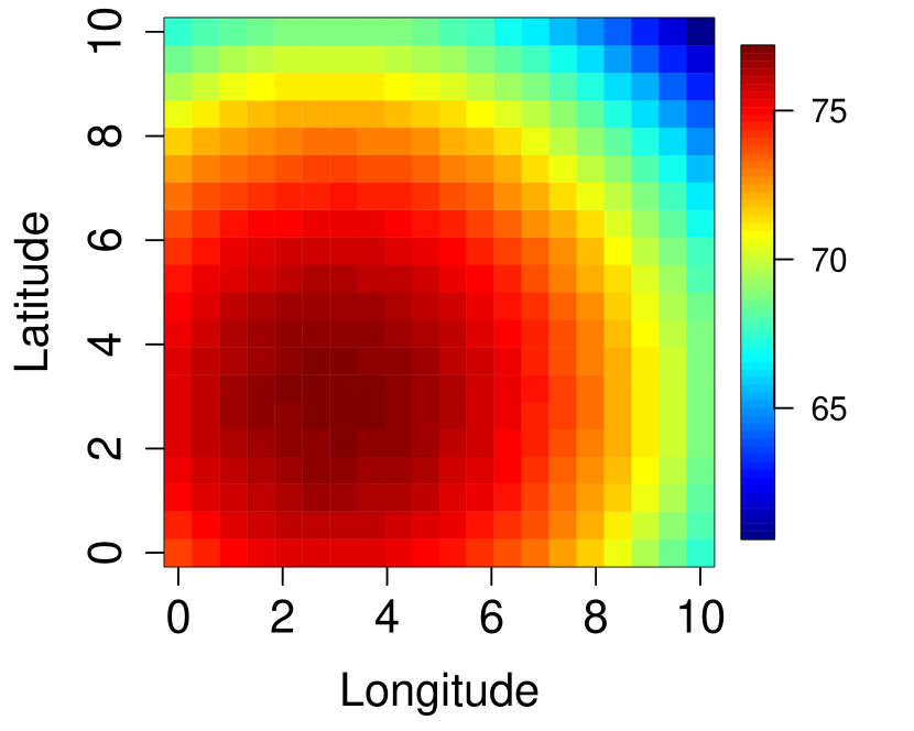
(a) True $a(\boldsymbol{x})$.

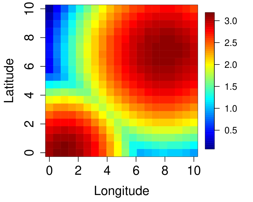
(b) True $b(\boldsymbol{x})$.

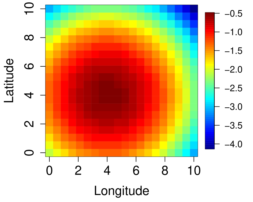
(c) True $s(\boldsymbol{x})$.

Figure 1: The true $a(\boldsymbol{x}_{i})$, $b(\boldsymbol{x}_{i})$ and $s(\boldsymbol{x}_{i})$ for the small-scale simulation study plotted on regular lattices.

This study consists of spatial locations on a $20\times 20$ regular lattice on $[0,10]\times[0,10]\subset\mathbb{R}^{2}$, resulting in a total of $n=400$ locations. The corresponding $a(\boldsymbol{x}_{i})$, $b(\boldsymbol{x}_{i})$ and $s(\boldsymbol{x}_{i})$ are set deterministically via the functions

$$a(\boldsymbol{x})= -0.5\cdot\log\left\{\textrm{det}(2\pi\boldsymbol{\Sigma}_{0})\right\}-0.5\cdot(\boldsymbol{x}-\boldsymbol{\mu}_{0})^{T}\boldsymbol{\Sigma}_{0}^{-1}(\boldsymbol{x}-\boldsymbol{\mu}_{0})+80,$$ (22)

$$\begin{split}b(\boldsymbol{x})=&0.083\cdot\log\Big{\{}0.4\cdot\textrm{det}(2\pi\boldsymbol{\Sigma}_{1})^{-\frac{1}{2}}\exp\left(-\frac{1}{2}(\boldsymbol{x}-\boldsymbol{\mu}_{1})^{T}\boldsymbol{\Sigma}_{1}^{-1}(\boldsymbol{x}-\boldsymbol{\mu}_{1})\right)\\ &+0.6\cdot\textrm{det}(\boldsymbol{\Sigma}_{2})^{-\frac{1}{2}}\exp\left(-\frac{1}{2}(\boldsymbol{x}-\boldsymbol{\mu}_{2})^{T}\boldsymbol{\Sigma}_{2}^{-1}(\boldsymbol{x}-\boldsymbol{\Sigma}_{2})\right)\Big{\}}+3.33,\end{split}$$ (23)

$$s(\boldsymbol{x})= -0.1\cdot\log\left\{\textrm{det}(2\pi\boldsymbol{\Sigma}_{3})\right\}-0.1\cdot(\boldsymbol{x}-\boldsymbol{\mu}_{3})^{T}\boldsymbol{\Sigma}_{3}^{-1}(\boldsymbol{x}-\boldsymbol{\mu}_{3}),$$ (24)

where

$$\boldsymbol{\mu}_{0} =\begin{pmatrix}3\\ 3\end{pmatrix},\ \boldsymbol{\Sigma}_{0}=\begin{pmatrix}3&0\\ 0&3\end{pmatrix},\ \boldsymbol{\mu}_{1}=\begin{pmatrix}1\\ 0\end{pmatrix},\ \boldsymbol{\Sigma}_{1}=\begin{pmatrix}0.5&0\\ 0&0.5\end{pmatrix},$$

$$\boldsymbol{\mu}_{2} =\begin{pmatrix}8\\ 7\end{pmatrix},\ \boldsymbol{\Sigma}_{2}=\begin{pmatrix}1&0\\ 0&1\end{pmatrix},\ \boldsymbol{\mu}_{3}=\begin{pmatrix}4\\ 4\end{pmatrix},\ \boldsymbol{\Sigma}_{3}=\begin{pmatrix}2&0\\ 0&2\end{pmatrix}.$$

Heat maps for $a(\boldsymbol{x})$, $b(\boldsymbol{x})$ and $s(\boldsymbol{x})$ on the spatial domain are displayed in Figure 1(a), 1(b), 1(c). Values of the GEV parameter are chosen so that the simulated observations mimic extreme daily precipitation levels in millimeters [Cooley & Sain, 2010]. In particular, the range of the shape parameters is $(0.016,0.6)$, which guarantees that the GEV distribution at each location has a finite mean. At each location $\boldsymbol{x}_{i}$, $n_{i}$ observations are simulated from $\operatorname{GEV}(a(\boldsymbol{x}_{i}),e^{b(\boldsymbol{x})},e^{s(\boldsymbol{x})})$ with $n_{i}$ drawn from a $\textrm{discrete Uniform}(20,50)$. No covariates are included in the mean functions of the spatial Gaussian processes, so each GP has one fixed mean parameter $\beta$ in the mean function.

We specify weakly informative Normal priors on the GP mean parameters: $\beta_{a}\sim\mathcal{N}(0,100)$, $\beta_{b}\sim\mathcal{N}(0,50)$, and $\beta_{s}\sim\mathcal{N}(0,20)$. Flat uniform priors are assumed for the remaining hyperparameters associated with the kernel function. For the Laplace method, $n_{\textrm{sim}}=10,000$ samples are drawn from $p(\boldsymbol{u}\mid\boldsymbol{y})$ in order to construct the posterior return-level distributions $p(z_{p}(\boldsymbol{x}_{i})\mid\boldsymbol{y})$ as described in Section 2.4. For the MCMC method, six Markov chains were run in parallel for 8000 iterations (including 4000 warm-ups) per chain. The effective sample sizes for all fixed and random effects range between $629$ and $38223$, with a mean of $18065$. We checked that all chains have mixed well based on the $\widehat{R}<1.01$ convergence metric advocated in Vehtari et al. [2021].

Posterior distributions of the hyperparameters are shown in Figure 2. Despite the agreement of posterior modes, the posterior distributions for $\beta_{a}$, $\beta_{b}$ and $\beta_{s}$ from MCMC have much longer tails than those from the Laplace method, and are therefore truncated for visibility of the plots in Figure 2(a), 2(d), and 2(g). The middle and right panels of Figure 2 show that the Laplace method results in lower posterior means for the variance parameters and higher posterior means for the inverse range parameters compared to MCMC. Furthermore, the Laplace method produces narrower posterior distributions, i.e., lower uncertainty, for all hyperparameters. This suggests that the Normal approximation for hyperparameters posterior in (13) might not be as precise. However, our interest lies in estimating the random effects and functions of them. As a result, we believe the estimated posteriors of interest $p(\boldsymbol{u}\mid\boldsymbol{y})$ are still accurate enough for inference purposes, which is supported by Figure 3 and 4.

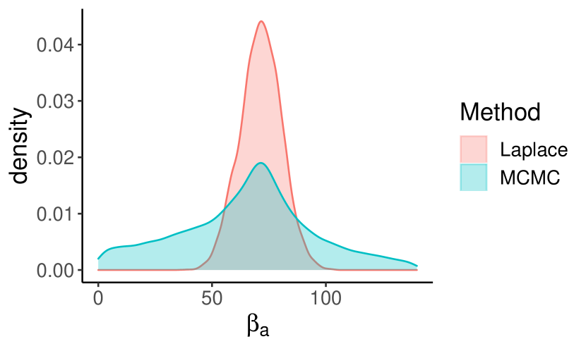
(a) Posterior distribution for $\beta_{a}$.

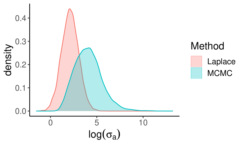
(b) Posterior distribution of $\log(\sigma_{a}^{2})$.

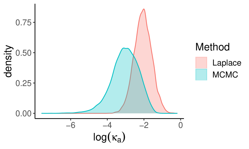
(c) Posterior distribution of $\log(\kappa_{a}^{2})$.

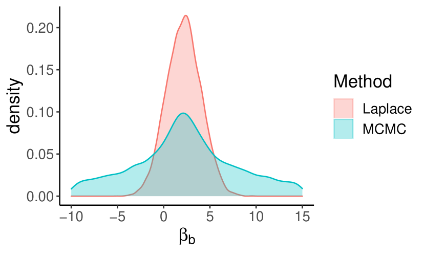
(d) Posterior distribution for $\beta_{b}$.

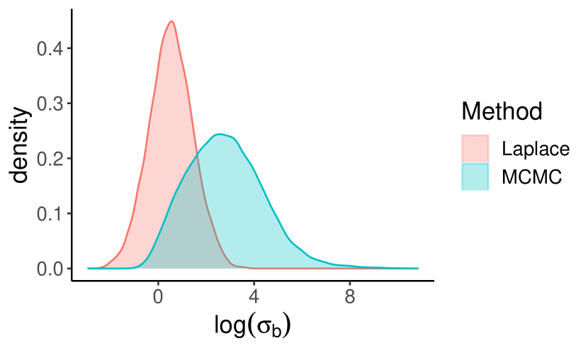
(e) Posterior distribution of $\log(\sigma_{b}^{2})$.

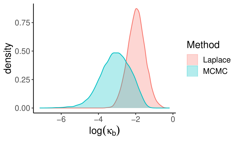
(f) Posterior distribution of $\log(\kappa_{b}^{2})$.

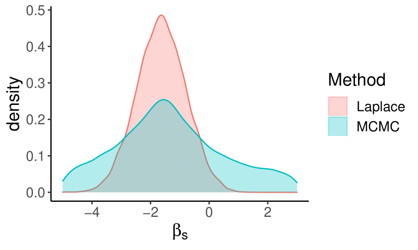
(g) Posterior distribution for $\beta_{s}$.

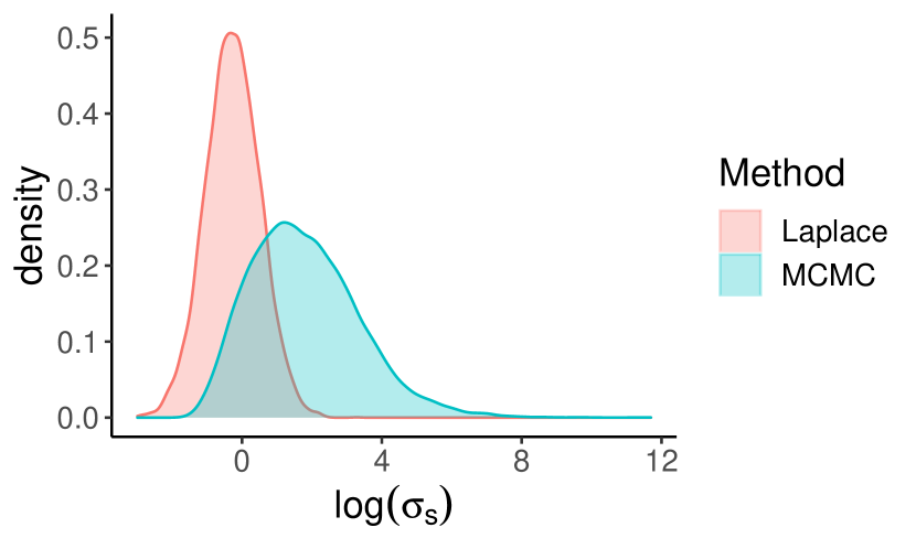
(h) Posterior distribution of $\log(\sigma_{s}^{2})$.

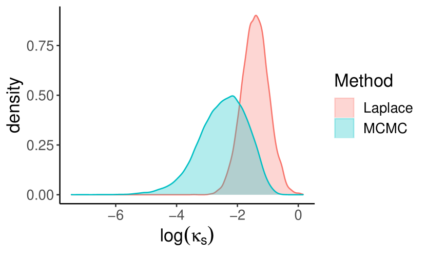
(i) Posterior distribution of $\log(\kappa_{s}^{2})$.

Figure 2: Posterior distributions of the hyperparameters $\boldsymbol{\theta}$ in the small-sale simulation study.

Figure 3(a), 3(b), 3(c), 3(e), 3(f) and 3(g) show the scatterplots of the posterior mean estimates of $a(\boldsymbol{x})$, $b(\boldsymbol{x})$ and $s(\boldsymbol{x})$ versus their true values using the two methods. The Laplace method slightly underestimates the location parameter and correspondingly overestimates the shape parameter at some locations. Further investigation shows that the locations at which the point estimate of $s(\boldsymbol{x})$ deviates the greatest from the truth are those lying on the boundary of the spatial domain. It is also noteworthy that the shape parameter is known to be particularly difficult to estimate [Schliep et al., 2010, Cooley & Sain, 2010]. Nevertheless, the same pattern occurs in MCMC which provides evidence for the accuracy of the Laplace method relative to the true posterior.

Next, we turn to the estimation of the meteorological quantity of interest, i.e., the return levels $z_{p}(\boldsymbol{x}_{i})$. At each location, the Bayesian point estimate of the $10$-year return level $z_{10}(\boldsymbol{x})$ is computed. Figure 3(d) and 3(h) show the estimates obtained from MCMC and the Laplace method as functions of the true return levels. Despite the slight overestimation of $s(\boldsymbol{x})$ at a few locations, point estimates of $z_{10}(\boldsymbol{x})$ align closely with the true values. This suggests that small bias in the estimation of the shape parameters has only a modest effect on the estimation of the marginal quantiles when the true shape parameter is close to 0 on the original scale. Thus, while the Laplace method is orders of magnitude faster than the MCMC, the accuracy of the point estimates are about the same.

(a) MCMC

(b) MCMC

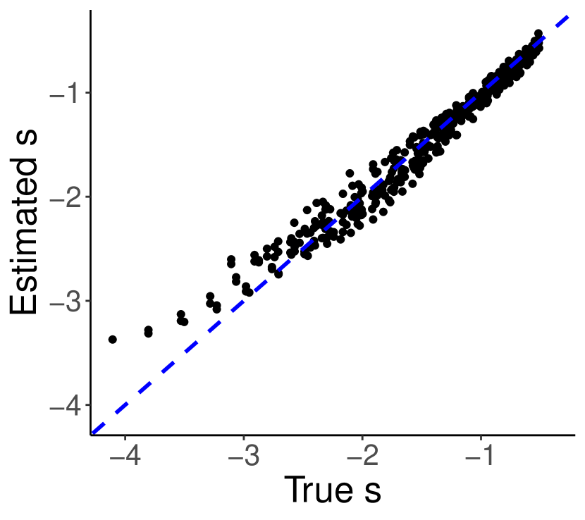
(c) MCMC

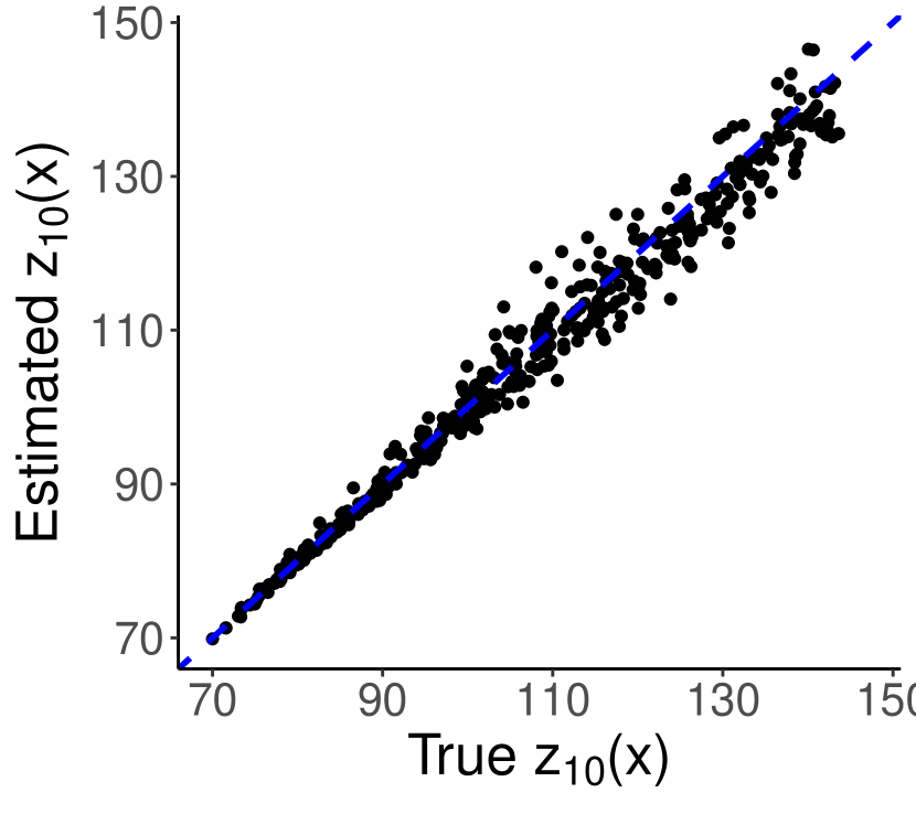
(d) MCMC

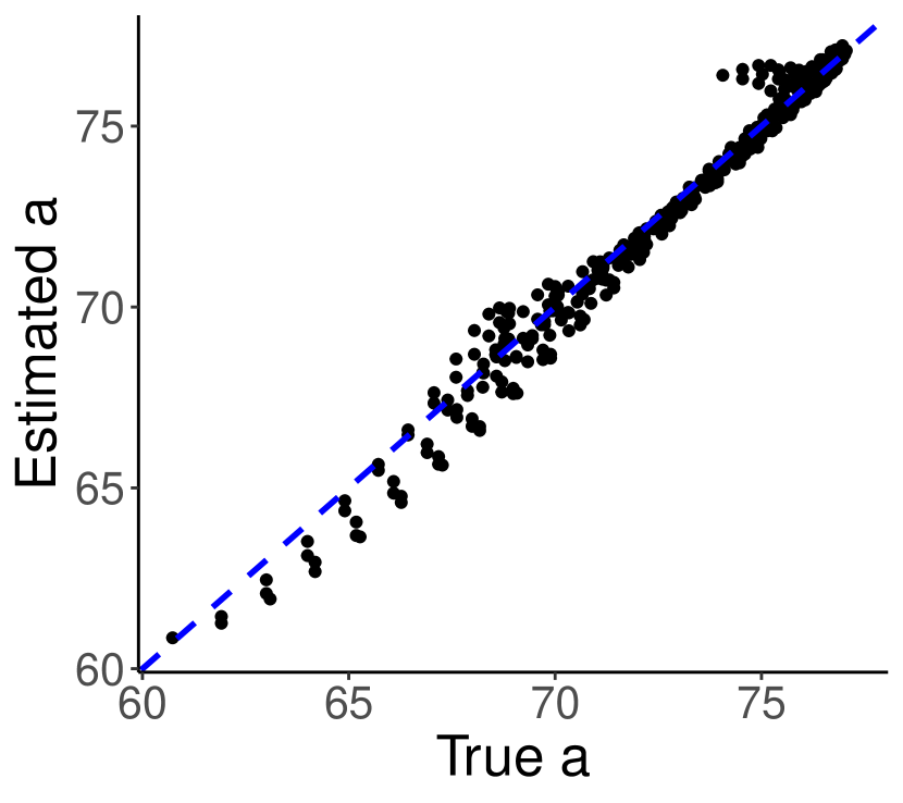
(e) Laplace

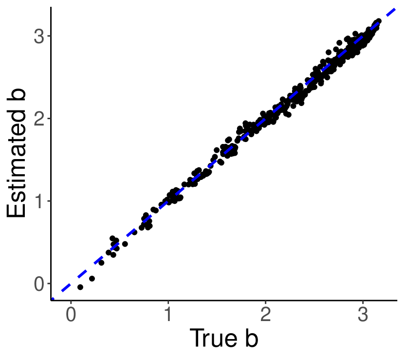
(f) Laplace

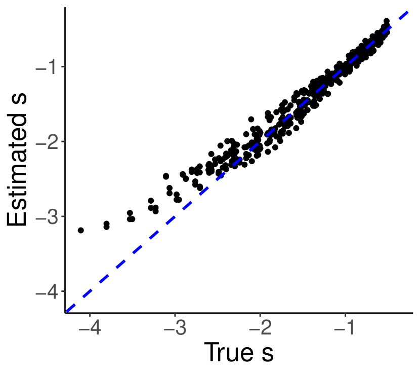
(g) Laplace

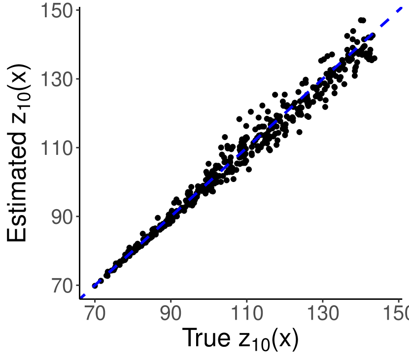
(h) Laplace

Figure 3: True GEV location parameters $a(\boldsymbol{x})$, scale parameters $b(\boldsymbol{x})$, shape parameters $s(\boldsymbol{x})$, and 10-year return levels $z_{10}(\boldsymbol{x})$ plotted against their estimates obtained using MCMC and Laplace.

As mentioned in Kass & Steffey [1989], the PEB approximation typically gives good estimates of the posterior mean of the random effects, but often underestimates their posterior variance. To assess this, Figure 4 examines the uncertainty estimates provided by the proposed method. The upper panel of Figure 4 shows the posterior standard deviations of the three GEV parameters at each point on the regular lattice. More uncertainty is observed on the boundary, especially at the corners, of the spatial domain. Assuming the MCMC samples are a good representation of the true posterior distributions, we see a satisfactory agreement between the posterior uncertainty from the Laplace method and that from MCMC, as shown in the lower panel of Figure 4 which plots the ratios between posterior standard deviations from Laplace and those from MCMC. This provides some justification for using the approximation (20) in this simulation study.

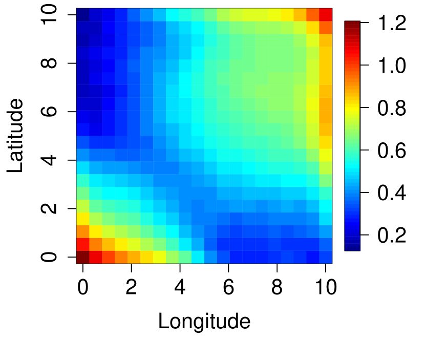
(a) Posterior SD of $a_{\textrm{La}}(\boldsymbol{x})$

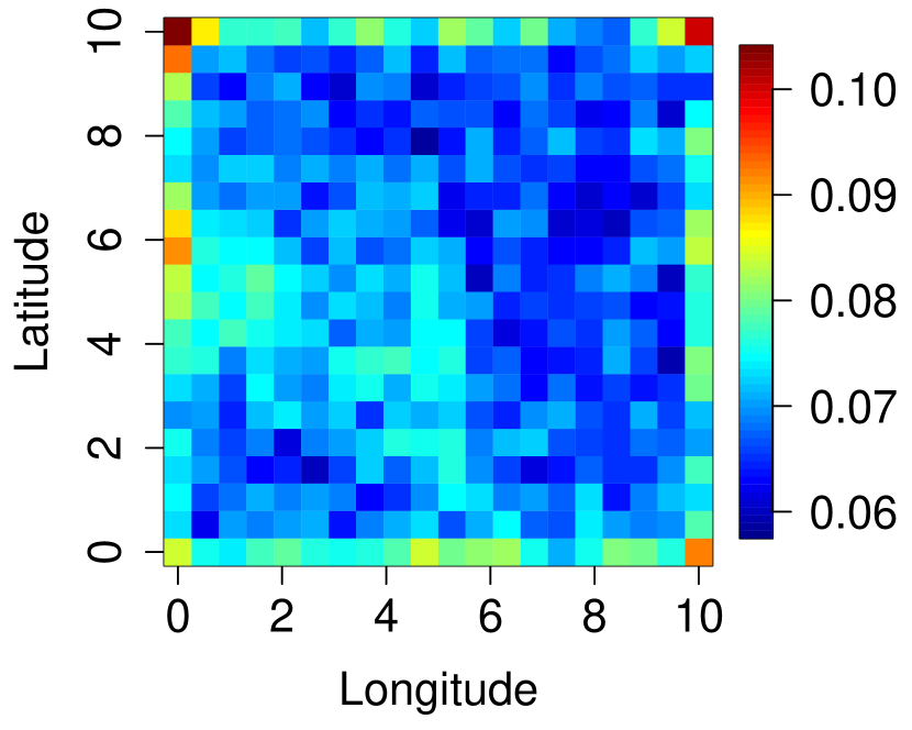
(b) Posterior SD of $b_{\textrm{La}}(\boldsymbol{x})$

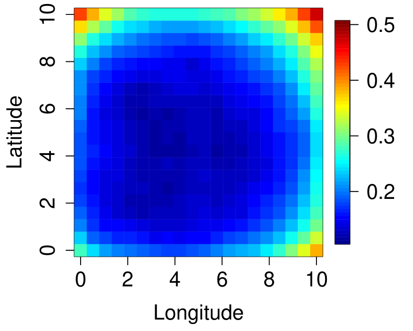
(c) Posterior SD of $s_{\textrm{La}}(\boldsymbol{x})$

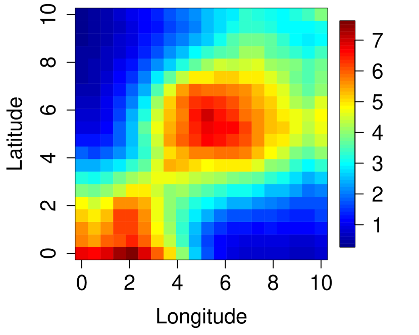
(d) Posterior SD of $z_{\textrm{La}}(\boldsymbol{x})$

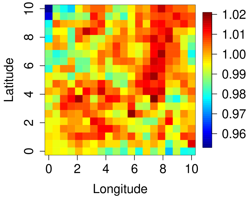
(e) $\frac{\textrm{Posterior SD of }a_{\textrm{La}}(\boldsymbol{x})}{\textrm{Posterior SD of }a_{\textrm{MCMC}}(\boldsymbol{x})}$

(f) $\frac{\textrm{Posterior SD of }b_{\textrm{La}}(\boldsymbol{x})}{\textrm{Posterior SD of }b_{\textrm{MCMC}}(\boldsymbol{x})}$

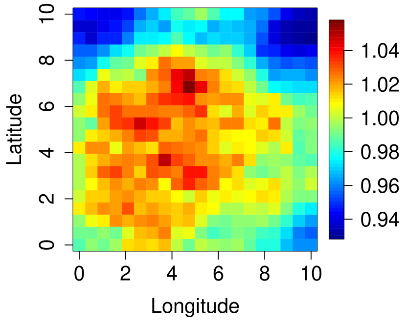
(g) $\frac{\textrm{Posterior SD of }s_{\textrm{La}}(\boldsymbol{x})}{\textrm{Posterior SD of }s_{\textrm{MCMC}}(\boldsymbol{x})}$

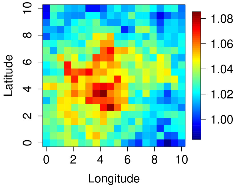
(h) $\frac{\textrm{Posterior SD of }z_{\textrm{La}}(\boldsymbol{x})}{\textrm{Posterior SD of }z_{\textrm{MCMC}}(\boldsymbol{x})}$

Figure 4: Upper panel: standard deviations of posterior samples of $a(\boldsymbol{x}_{i})$, $b(\boldsymbol{x}_{i})$, $s(\boldsymbol{x}_{i})$ and $z_{10}(\boldsymbol{x})$ from the Laplace approach plotted on the regular lattice. Lower panel: ratios between the posterior standard deviations obtained from the Laplace method and those from MCMC.

Table 1 reports the numerical summary of accuracy results as well as computational speed. The evaluation metrics are the mean absolute errors for $a(\boldsymbol{x})$, $b(\boldsymbol{x})$ and $s(\boldsymbol{x})$ at the $n=400$ spatial locations, the Kolmogorov-Smirnov (KS) statistic that checks the agreement between posterior samples of $z_{10}(\boldsymbol{x})$ from Laplace and those from MCMC, as well as mean computation times with standard deviations. At each location $\boldsymbol{x}$, the KS statistic is obtained using the R function ks.test() to check whether two posterior samples of $z_{10}(\boldsymbol{x})$ are drawn from the same distribution. The mean and standard deviation of the $400$ KS statistics are reported, which do not indicate any strong evidence that the posteriors of $z_{10}(\boldsymbol{x})$ given by the Laplace method deviate from those given by MCMC. Model fitting was carried out using R 3.6.2 on a computer cluster with six 2.7GHz Xeon(R) CPUs (E5-4650) and 1GB memory per CPU. Note that the Laplace method was performed on only one CPU whereas MCMC utilizes all six. The computation time for the Laplace method is reported from 20 repetitions of model fitting and sampling using the same simulated dataset, whereas that for MCMC is based on the elapsed times of the 6 parallel chains. Compared to MCMC, our method is about three orders of magnitude faster while obtaining similar accuracy for estimating $a(\boldsymbol{x})$, $b(\boldsymbol{x})$ and $s(\boldsymbol{x})$.

	MCMC	Laplace
$\operatorname{MAE}\big{(}\widehat{a}(\boldsymbol{x})\big{)}=\frac{\sum_{i=1}^{n}|a(\boldsymbol{x}_{i})-\widehat{a}(\boldsymbol{x}_{i})|}{n}$	0.384	0.384
$\operatorname{MAE}\big{(}\widehat{b}(\boldsymbol{x})\big{)}=\frac{\sum_{i=1}^{n}|b(\boldsymbol{x}_{i})-\widehat{b}(\boldsymbol{x}_{i})|}{n}$	0.0476	0.0506
$\operatorname{MAE}\big{(}\widehat{s}(\boldsymbol{x})\big{)}=\frac{\sum_{i=1}^{n}|s(\boldsymbol{x}_{i})-\widehat{s}(\boldsymbol{x}_{i})|}{n}$	0.102	0.111
$\operatorname{MAE}\big{(}\widehat{z}_{10}(\boldsymbol{x})\big{)}=\frac{\sum_{i=1}^{n}|z(\boldsymbol{x}_{i})-\widehat{z}(\boldsymbol{x}_{i})|}{n}$	2.262	2.182
Mean runtime (SD)	225091($9110$)s	71($0.4$)s
Mean KS statistic of $z_{10}(\boldsymbol{x})$ (SD)	$0.0490(0.0138)$

Table 1: Comparison between MCMC and the Laplace method.

3.2 Large-Scale Study on Rough Surfaces

The simulation study above has examined the performance of the proposed Laplace method when the GEV parameters are all simulated from relatively smooth surfaces. Here, we consider a more difficult case in which the parameter surfaces are more “patchy” (as shown in Figure 5) and where the number of locations is an order of magnitude larger than the previous simulation study. The parameters $a(\boldsymbol{x})$, $b(\boldsymbol{x})$ and $s(\boldsymbol{x})$ are simulated from Gaussian random fields with an exponential covariance kernel function on a $80\times 80$ regular lattice on $[0,60]\times[0,60]\subset\mathbb{R}^{2}$:

$$a(\boldsymbol{x}) \sim\mathcal{GP}\big{(}70,\ k(\boldsymbol{x},\boldsymbol{x}^{\prime}\mid 8,20)\big{)}$$ (25)

$$b(\boldsymbol{x}) \sim\mathcal{GP}\big{(}a(\boldsymbol{x})/10-4,\ k(\boldsymbol{x},\boldsymbol{x}^{\prime}\mid 0.01,20)\big{)}$$ (26)

$$s(\boldsymbol{x}) \sim\mathcal{GP}\big{(}-a(\boldsymbol{x})/10+5,\ k(\boldsymbol{x},\boldsymbol{x}^{\prime}\mid 0.01,30)\big{)},$$ (27)

where $\sigma$ and $\lambda$ in $k(\boldsymbol{x},\boldsymbol{x}^{\prime}\mid\sigma,\lambda)$ are the scale and range parameters of the kernel function, respectively. Simulation is carried out using the rgp() function in the SpatialExtremes package [Ribatet et al., 2022]. The other aspects of the simulation study – e.g., data generation mechanism, prior specification, and other modelling setups – are the same as those in Section 3.1.

In this simulation, $\boldsymbol{u}$ consists of three random effects at each of the $6400$ spatial locations, resulting in a total of $19200$ random effects. As it is computationally infeasible to store and invert the $19200\times 19200$ dimensional covariance matrix to sample from $p(\boldsymbol{u}\mid\boldsymbol{y})$, the Delta method is used to compute only the posterior mean and standard deviation of $z_{10}(\boldsymbol{x}_{i})$ at each spatial location, as discussed in Section 2.5. Model fitting is run on the same computer cluster described in Section 3.1, except with a single CPU and 90Gb of memory. The total computational time is $22$ hours. As for MCMC, running 100 iterations per parallel chain using rstan took over a week. This was not nearly enough for the MCMC to converge, thus highlighting the immense computational savings offered by the Laplace approximation.

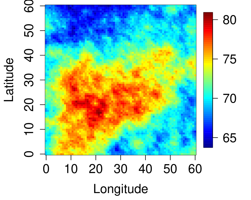
(a) True $a(\boldsymbol{x})$.

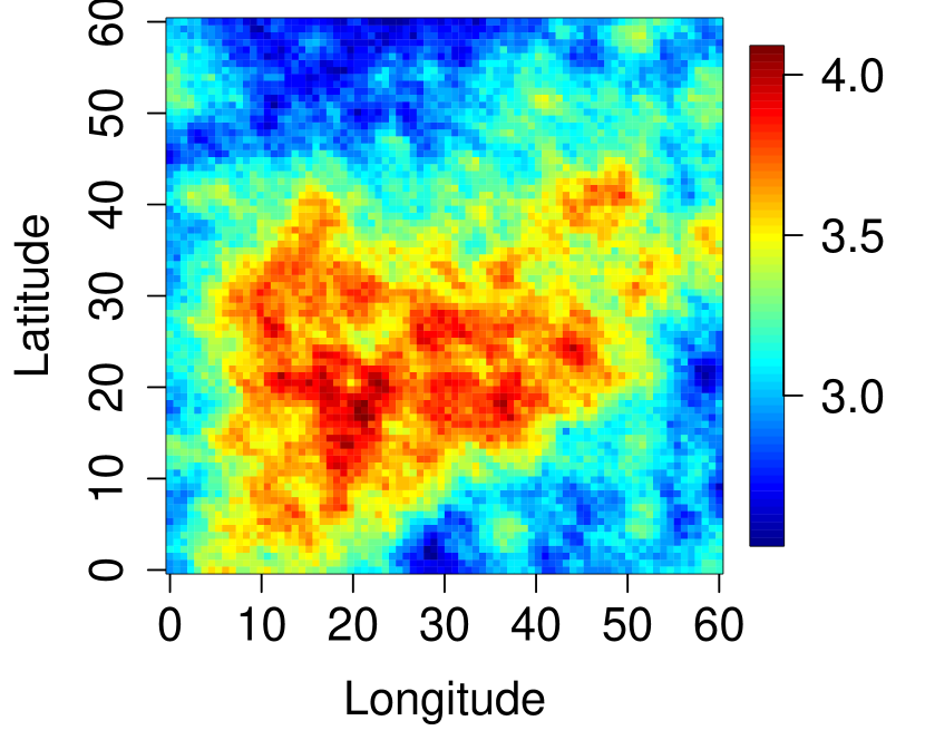
(b) True $b(\boldsymbol{x})$.

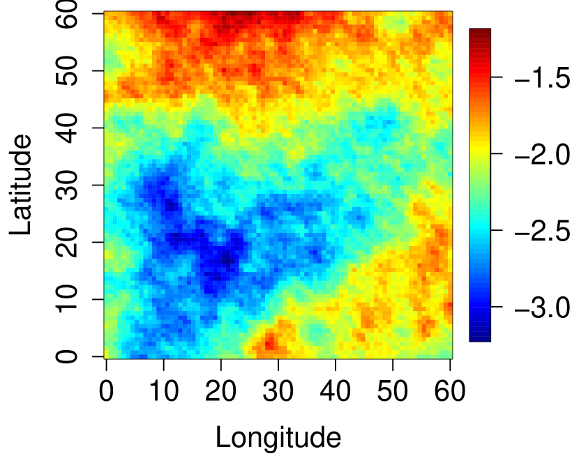
(c) True $s(\boldsymbol{x})$.

Figure 5: The true $a(\boldsymbol{x}_{i})$, $b(\boldsymbol{x}_{i})$ and $s(\boldsymbol{x}_{i})$ for the large-scale simulation study simulated from three Gaussian random fields.

Figure 6 compares the posterior mean estimates of all GEV parameters and the 10-year return levels from the Laplace method to their true values. The overall trends of both the location parameter $a(\boldsymbol{x})$ and scale parameter $b(\boldsymbol{x})$ are captured well by the corresponding posterior mean estimates. The shape parameter tends to be slightly overestimated when the true value is small, which has been also observed in Figure 3(c). Finally, the posterior mean estimates of the 10-year return levels, the quantity of interest, align well with the true values at the majority of the locations. These results demonstrate both the computational feasibility of the Laplace method as well as the accuracy of the obtained point estimates.

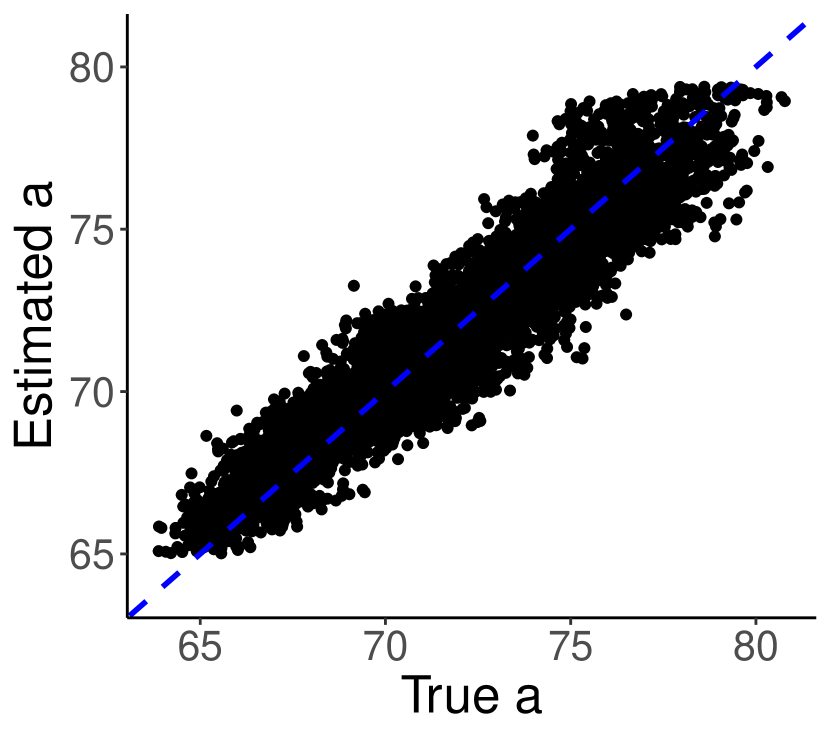
(a) Laplace

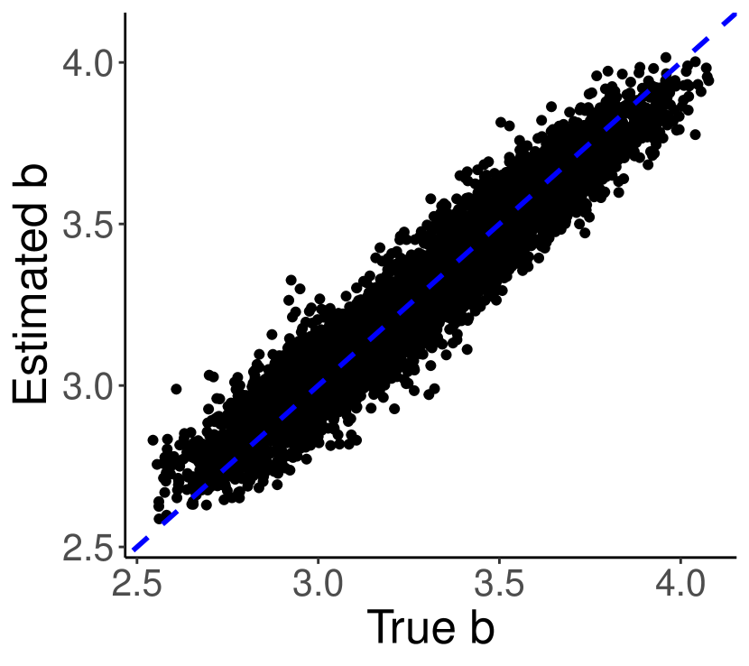
(b) Laplace

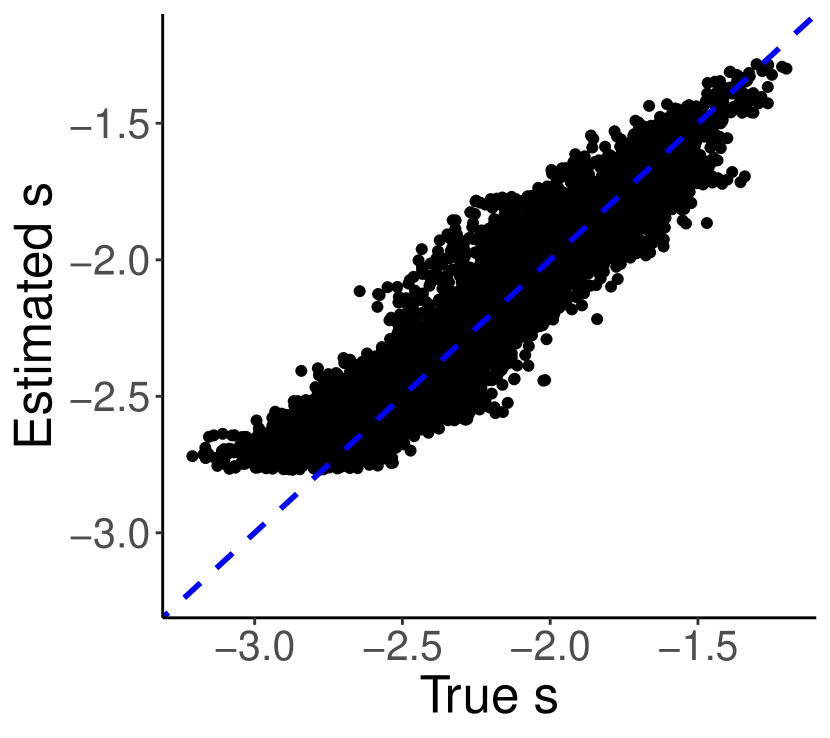
(c) Laplace

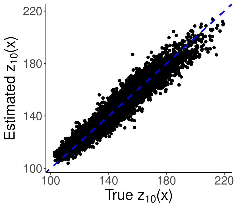
(d) Laplace

Figure 6: True GEV location parameters $a(\boldsymbol{x})$, scale parameters $b(\boldsymbol{x})$, shape parameters $s(\boldsymbol{x})$, and 10-year return levels $z_{10}(\boldsymbol{x})$ plotted against their estimates obtained using the Laplace method when the true parameter surfaces are unsmooth.

4 Case Study

Here, we study a real data set of monthly total snowfall in Canada from January 1987 to December 2021, which is publicly available through Environment and Climate Change Canada [2022]. The monthly total snowfall at a location is the amount of frozen precipitation (in cm), including snow and ice pellets, observed throughout a month. The goal of this study is to produce a cross-country map of 10-year return levels $z_{10}(\boldsymbol{x})$ of extreme monthly total snowfall at the observed locations.

The dataset includes $3833$ weather stations plotted in Figure 7(a). In Figure 7(b), the data are gridded into $1^{\circ}\times 1^{\circ}$ cells. We only include cells in which there are at least 10 years of observations, and in line with extreme value theory, use the maximum yearly records of monthly snowfall in each cell as the response values. This results $n=509$ spatial locations (grid cells) each with at least 10 extreme value observations. No additional covariates are included in the model. The triangulated mesh for SPDE approximation is superimposed on the map in Figure 7(b). A non-convex boundary is built for the mesh, leaving out a hole in the region of Hudson Bay due to the physical boundary it creates in the spatial domain. This results in $n^{\prime}=1565$ nodes, each of which will have separate estimated GEV random effects. Prediction at unobserved locations is straightforward using the Gaussian process methodology [Rasmussen & Williams, 2006] described in B.

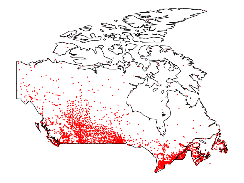
(a) All locations

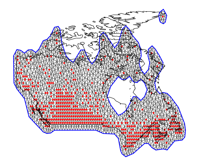
(b) Gridded locations on the mesh

Figure 7: (a): All $3833$ locations at which data was collected from 1987 to 2021. (b): $509$ locations at which at least 10 years of data was recorded after gridding.

4.1 Model Selection

We first fit a GEV-GP model with all GEV parameters as spatial random effects, which is denoted by $M_{\textrm{abs}}$. The point estimates $\widehat{s}(\boldsymbol{x})$ at all locations have a small range from $-8.1$ to $-8.0$, suggesting that the model with spatially varying $s(\boldsymbol{x})$ might not be needed. Therefore, we reduce the model complexity by having the shape parameter as a fixed effect $s$ across space, and denote this model by $M_{\textrm{ab}}$. A Normal prior $\mathcal{N}(-5,5)$ is imposed on $s$. Furthermore, we compare model $M_{\textrm{ab}}$ to the simplest spatial extreme model $M_{\textrm{a}}$ with only $a(\boldsymbol{x})$ spatially varying. The model with random scale parameter and fixed location and shape parameters, i.e., $M_{\textrm{b}}$, is not considered here as the spatial variation of $a(\boldsymbol{x})$ contributes greatly to the observation variation across different locations.

The fit of models $M_{\textrm{ab}}$ and $M_{\textrm{a}}$ to the snowfall dataset is evaluated using a model checking procedure described below. The posterior predictive distribution of maximum monthly total snowfall $y_{\star}$ at spatial location $\boldsymbol{x}_{\star}$ is given by

$$\begin{split}p(y_{\star}\mid\boldsymbol{y})&=\int p\big{(}y_{\star}\mid a(\boldsymbol{x}_{\star}),b(\boldsymbol{x}_{\star}),s(\boldsymbol{x}_{\star})\big{)}\times\\ &\ \ \ \ \ \ \ \ \ \ \ \ \ \ \ \ \ p\big{(}a(\boldsymbol{x}_{\star}),b(\boldsymbol{x}_{\star}),s(\boldsymbol{x}_{\star})\mid\boldsymbol{y}\big{)}\mathop{}\!{\operator@font{d}}a(\boldsymbol{x}_{\star})\mathop{}\!{\operator@font{d}}b(\boldsymbol{x}_{\star})\mathop{}\!{\operator@font{d}}s(\boldsymbol{x}_{\star}).\end{split}$$ (28)

Agreement between model and data can be measured by comparing a chosen test statistic computed using replicated data drawn from the posterior predictive distribution, denoted by $T(y^{\textrm{rep}}\mid\boldsymbol{x})$, and that computed from the observed data, denoted by $T(y^{\textrm{obs}}\mid\boldsymbol{x})$. If the model is correctly specified, then $T(y^{\textrm{rep}}\mid\boldsymbol{x})\approx T(y^{\textrm{obs}}\mid\boldsymbol{x})$. The calculations of the posterior predictive distribution (28) and $T(y^{\textrm{rep}}\mid\boldsymbol{x})$ are detailed in B.

The test statistics chosen here are the sample median and the $10$% upper sample quantile, i.e. the 10-year return rate. Figure 8 plots $T(y^{\textrm{rep}}\mid\boldsymbol{x})$ versus $T(y^{\textrm{obs}}\mid\boldsymbol{x})$ for both models $M_{\textrm{ab}}$ and $M_{\textrm{a}}$, where each dot represents the test statistic calculated at a location, and lack of fit is indicated by departures from the $45^{\circ}$ blue dashed line. Reading the plots, it is clear that model $M_{ab}$ outperforms $M_{a}$. This observation underscores the importance of having the ability to model more than just the location parameter of the GEV distribution as spatially varying, which cannot be accomplished using the INLA methodology. Consequently, the remaining analyses in this section will be performed with model $M_{\textrm{ab}}$.

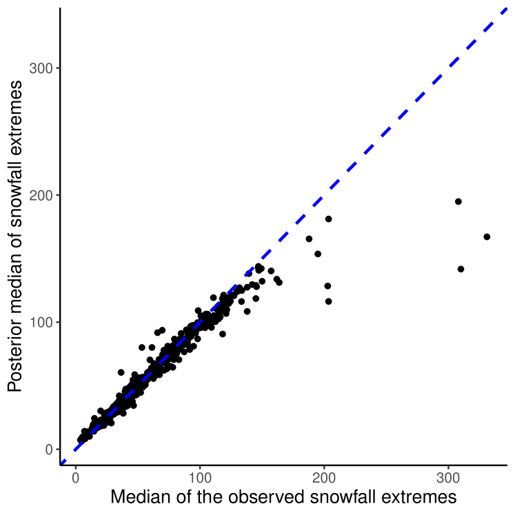
(a) Model $M_{\textrm{ab}}$: random $a(\boldsymbol{x})$ and $b(\boldsymbol{x})$
Test quantity: median.

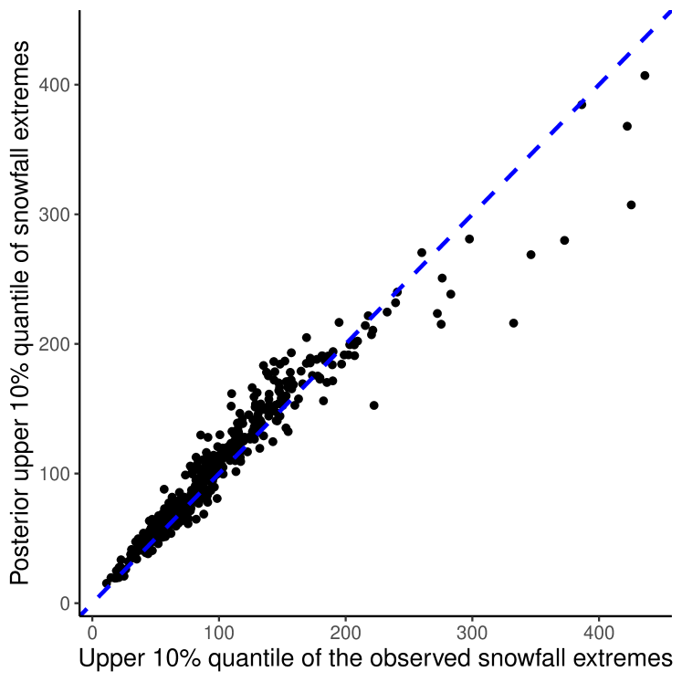
(b) Model $M_{\textrm{ab}}$: random $a(\boldsymbol{x})$ and $b(\boldsymbol{x})$.
Test quantity: upper $10$% quantile

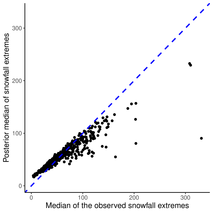
(c) Model $M_{\textrm{a}}$: random $a(\boldsymbol{x})$, fixed $b$.
Test quantity: median

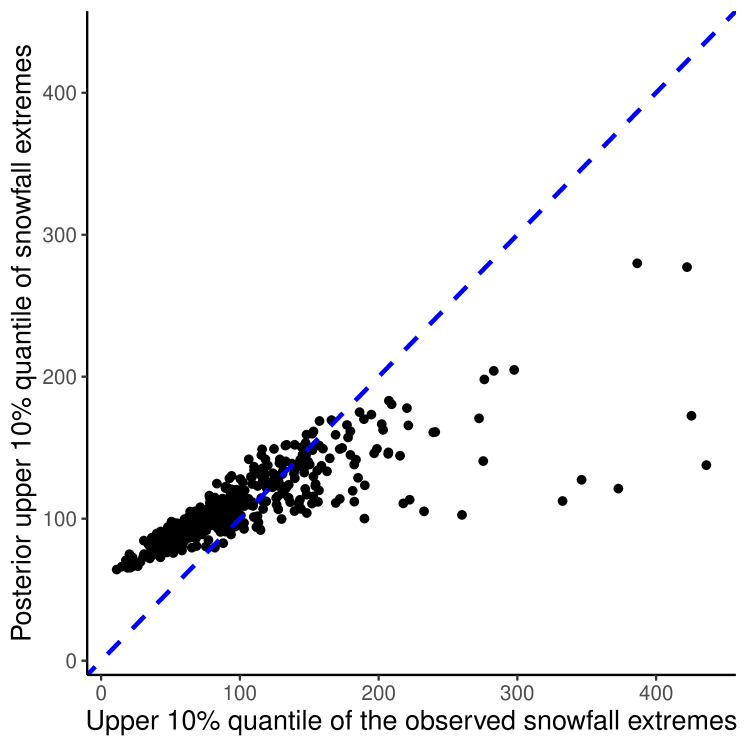
(d) Model $M_{\textrm{a}}$: random $a(\boldsymbol{x})$, fixed $b$.
Test quantity: upper $10$% quantile

Figure 8: Predictive test quantity $\boldsymbol{T}(\boldsymbol{y}^{\textrm{rep}})$ versus realized test quantity $\boldsymbol{T}(\boldsymbol{y})$. Each black dot represent a location. Upper panel: Model with both $a(\boldsymbol{x})$ and $b(\boldsymbol{x})$ as spatial random effects. Lower panel: Model with only $a(\boldsymbol{x})$ random. Left panel: Predictive medians versus realized medians. Right panel: Predictive upper $10$% quantiles versus realized upper $10$% quantiles.

4.2 Parameter Inference

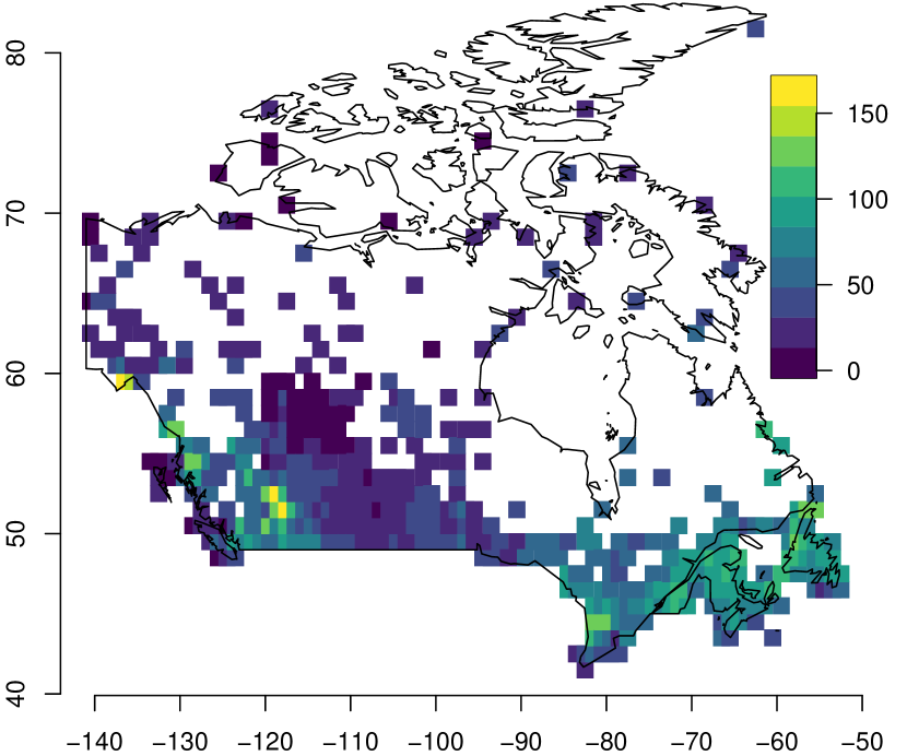
(a) Posterior mean of $a(\boldsymbol{x})$.

(b) Posterior standard deviation of $a(\boldsymbol{x})$.

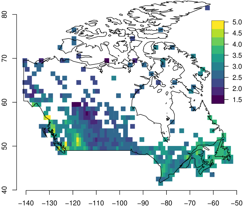
(c) Posterior mean of $b(\boldsymbol{x})$.

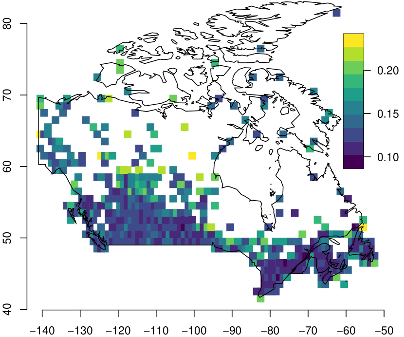
(d) Posterior standard deviation of $b(\boldsymbol{x})$.

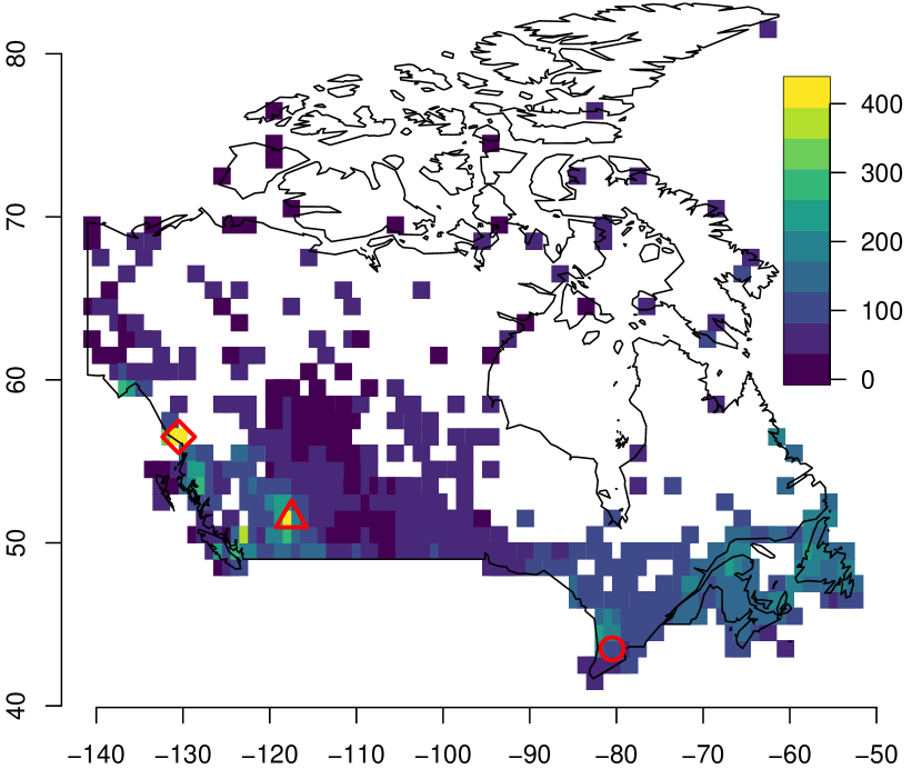
(e) Posterior mean of 10-year return levels $z_{10}(\boldsymbol{x})$.

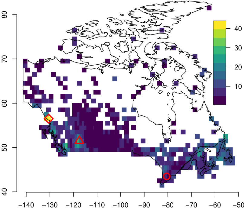
(f) Posterior standard deviation of $z_{10}(\boldsymbol{x})$.

Figure 9: Posterior means and standard deviations of $a(\boldsymbol{x})$, $b(\boldsymbol{x})$, and $z_{10}(\boldsymbol{x})$.

The posterior means and standard deviations of model parameters at each location are plotted on in Figure 9(a), 9(b), 9(c), 9(d). The posterior mean estimate of $s$ is $-7.7$ with a standard error of $1.54$, which suggests a lighter tail for the GEV distribution. Spatial patterns are observed for the values of $\widehat{a}(\boldsymbol{x})=E[a(\boldsymbol{x})\mid\boldsymbol{y}]$ and $\widehat{b}(\boldsymbol{x})=E[b(\boldsymbol{x})\mid\boldsymbol{y}]$ across Canada, with higher values of $\widehat{a}(\boldsymbol{x})$ and $\widehat{b}(\boldsymbol{x})$ in the Rocky mountains region in British Columbia and south of Alberta. We note that the uncertainty is higher for $b(\boldsymbol{x})$ in southern Nunavut and the southeast of Northwest Territories, where data is most sparse. Plotted in Figure 9(e) and 9(f) are the posterior $10$-year return level estimates $\widehat{z}_{10}(\boldsymbol{x})=E[z_{10}(\boldsymbol{x})\mid\boldsymbol{y}]$ and their corresponding uncertainty levels. These two maps provide a practical guide to interpret the risk of extreme snowfall across Canada. For example, the posterior mean estimate of 10-year return level at the coordinates $\boldsymbol{x}=(-80.5^{\circ},43.5^{\circ})$ in Waterloo, ON (marked by the red circle in Figure 9(e) and 9(f)) being $129.12$cm means that it takes an average of $10$ years before one observes a monthly total snowfall as extreme as $129.12$cm at this location. The 10-year return level can also be interpreted as a $10$% chance of observing such extreme monthly total snowfalls in any year at a given location. The same claim about coordinates $\boldsymbol{x}=(-117.5^{\circ},51.5^{\circ})$ in Glacier National Park in BC (marked by the red triangle) would be true for a monthly total snowfall as extreme as $377.40$ cm. Reading Figure 9(f), the estimate of the former location is relatively more precise compared to the latter one. From the uncertainty maps we can also identify locations where more observations may be needed to attain a practical level of precision, e.g., at $\boldsymbol{x}=(-130.5^{\circ},56.5^{\circ})$ near Granduc, BC (marked by the red diamond).

5 Discussion

In this paper we develop a computationally efficient method of Bayesian inference for fitting GEV-GP models, which have a wide range of applications in studying weather extremes. The proposed method applies the Laplace approximation for calculating the marginal likelihood and a Normal approximation based on a Taylor expansion to obtain the posterior distributions of the random effects. Scalability to many thousand spatial observations is achieved using a sparsity-inducing approximation to the spatial precision matrix. An efficient implementation of our method is provided in the R/ C++ package SpatialGEV [Chen et al., 2021]. Through simulation studies, we have shown that the proposed approximation is highly accurate and significantly faster than a state-of-the-art MCMC algorithm commonly used to fit hierarchical models such as the GEV-GP. The INLA method is a popular alternative to MCMC which has been used successfully in many analyses of weather extremes [e.g., Opitz et al., 2018, Castro-Camilo et al., 2019, 2020]. However, INLA cannot be used for GEV-GP models with two or more spatial random effects. Such flexibility can be crucial for accurate prediction of weather extreme values, as demonstrated in the analysis of extreme snowfall in Section 4.

We adopted a simple Taylor approximation for the conditional posterior distribution of the random effects $p(\boldsymbol{u}\mid\boldsymbol{\theta},\boldsymbol{y})$ given the fixed parameters $\boldsymbol{\theta}$ of the GEV-GP model. In a sense, we have assumed that it is sufficient for estimation accuracy and precision to condition on the posterior mode of the hyperparameters. This approach might result in underestimation of the random effects uncertainty when the posterior distribution of the hyperparameters is wide. Alternatively, a second-order Laplace approximation can be applied to potentially increase the precision, but the cost entailed to computing the second order term demands a trade-off between speed and precision. Numerical quadrature techniques can also be used to integrate over multiple representative values of the hyperparameters, resulting in a more precise estimation of the posterior distribution of the random effects. Applying such methods requires careful choice of the quadrature nodes and weights and other computational considerations. Stringer [2021] has implemented an adaptive Gauss-Hermite quadrature technique on a flexible class of latent Gaussian models. It is of interest to investigate its applicability to the GEV-GP model.

A fast inference method is important for the modelling and analysis of datasets containing a large number of spatial locations, especially when numerical procedures are required to work with an intractable form of the posterior distribution. Our method can work with both dense covariance matrices in the latent Gaussian processes, which scale poorly to large datasets due to the $\mathcal{O}(n^{3})$ cost of covariance matrix inversions, and sparse matrices that approximate the dense covariance matrix. Indeed, computational complexity can be improved by either introducing sparsity in the covariance matrices or by reducing their dimensionality. Methods that adopt the former approach typically involve assumptions about the dependence structure of the random effects, such as the SPDE approximation for the covariance matrix employed in this paper and in the R-INLA implementation. An example of the latter approach, which is another line of research, is the inducing point method within the variational inference framework [Quiñonero-Candela & Rasmussen, 2005, Snelson & Ghahramani, 2006, Titsias & Lawrence, 2010] which has been widely used in Gaussian process regression with tens of thousands of observations, and has also been applied on some versions of the latent Gaussian model with non-Gaussian likelihoods [e.g. Gal et al., 2015, Bonilla et al., 2019]. These methods in the Gaussian process literature are appealing from a theoretical point of view, but challenges remain in finding the optimal variational distribution that approximates the true posterior well. Extending these methods to the GEV-GP setting is a promising direction for future work.

Declaration of Interest

None.

Appendix A Estimation of Functions of Random Effects and Hyperparameters

Consider any non-linear vector-valued function $\boldsymbol{\eta}(\boldsymbol{u},\boldsymbol{\theta}):\mathbb{R}^{\textrm{dim}(\boldsymbol{u})+\textrm{dim}(\boldsymbol{\theta})}\to\mathbb{R}^{m}$. Once samples have been drawn from $\widetilde{p}(\boldsymbol{\theta}\mid\boldsymbol{y})$ and $\widetilde{p}(\boldsymbol{u}\mid\boldsymbol{y})$, which are computed using the method in Section 2, samples of $p(\boldsymbol{\eta}(\boldsymbol{u},\boldsymbol{\theta})\mid\boldsymbol{y})$ are obtained by taking non-linear transformations of samples $\boldsymbol{u}^{s}$ and $\boldsymbol{\theta}^{s}$. However, when the number of locations $n$ is large, it is extremely costly to store in memory the covariance matrix of $\widetilde{p}(\boldsymbol{u}\mid\boldsymbol{y})$ whose dimension is a multiple of $n$, and to sample repeatedly from a multivariate normal distribution of the same dimension. Applying the Delta method,

$$\boldsymbol{\eta}(\boldsymbol{u},\boldsymbol{\theta}) \approx\boldsymbol{\eta}(\boldsymbol{u}_{\widehat{\boldsymbol{\theta}}},\widehat{\boldsymbol{\theta}})+\boldsymbol{J}_{\boldsymbol{\eta}\circ\boldsymbol{u}}\cdot(\boldsymbol{\theta}-\widehat{\boldsymbol{\theta}}),$$ (29)

$$\widehat{\boldsymbol{V}}_{\boldsymbol{\eta}}(\boldsymbol{\theta}) \approx\boldsymbol{J}_{\boldsymbol{\eta}}\widehat{\boldsymbol{V}}_{\boldsymbol{u},\boldsymbol{\theta}}(\widehat{\boldsymbol{\theta}})\boldsymbol{J}_{\boldsymbol{\eta}}^{T},$$ (30)

where

$$\boldsymbol{u}_{\widehat{\boldsymbol{\theta}}} =\textrm{argmax}_{\boldsymbol{u}}G(\boldsymbol{u};\widehat{\boldsymbol{\theta}}),$$ (31)

$$\boldsymbol{J}_{\boldsymbol{\eta}\circ\boldsymbol{u}} =\boldsymbol{J}_{\boldsymbol{\eta}}\cdot\begin{pmatrix}\boldsymbol{J}_{u}\\ \boldsymbol{I}\end{pmatrix},$$ (32)

$$\boldsymbol{J}_{\boldsymbol{\eta}} =\left.\begin{pmatrix}\left(\frac{\partial\eta_{1}}{\partial\boldsymbol{u}}\right)^{T}&\left(\frac{\partial\eta_{1}}{\partial\boldsymbol{\theta}}\right)^{T}\\ \vdots&\vdots\\ \left(\frac{\partial\eta_{m}}{\partial\boldsymbol{u}}\right)^{T}&\left(\frac{\partial\eta_{m}}{\partial\boldsymbol{\theta}}\right)^{T}\end{pmatrix}\right|_{\boldsymbol{u}=\boldsymbol{u}_{\widehat{\boldsymbol{\theta}}},\boldsymbol{\theta}=\widehat{\boldsymbol{\theta}}},$$ (33)

$$\boldsymbol{J}_{\boldsymbol{u}} =\left.\left[\frac{\partial}{\partial\boldsymbol{\theta}}u_{\boldsymbol{\theta},1}\cdots\frac{\partial}{\partial\boldsymbol{\theta}}u_{\boldsymbol{\theta},3n}\right]^{T}\right|_{\boldsymbol{\theta}=\widehat{\boldsymbol{\theta}}}$$ (34)

$$=\left.-\left[\left(\frac{\partial^{2}}{\partial\boldsymbol{u}\partial\boldsymbol{u}^{T}}G(\boldsymbol{u}_{\boldsymbol{\theta}},\boldsymbol{\theta})\right)^{-1}\left(\frac{\partial^{2}}{\partial\boldsymbol{u}\partial\boldsymbol{\theta}^{T}}G(\boldsymbol{u}_{\boldsymbol{\theta}},\boldsymbol{\theta})\right)\right]\right|_{\boldsymbol{\theta}=\widehat{\boldsymbol{\theta}}},$$ (35)

$$\widehat{\boldsymbol{V}}_{\boldsymbol{u},\boldsymbol{\theta}}(\widehat{\boldsymbol{\theta}}) =\begin{pmatrix}\widehat{\boldsymbol{V}}_{\boldsymbol{u}}(\widehat{\boldsymbol{\theta}})+\boldsymbol{J}_{\boldsymbol{u}}\widehat{\boldsymbol{V}}_{\boldsymbol{\theta}}\boldsymbol{J}_{\boldsymbol{u}}^{T}&\boldsymbol{J}_{\boldsymbol{u}}\widehat{\boldsymbol{V}}_{\boldsymbol{\theta}}\\ \widehat{\boldsymbol{V}}_{\boldsymbol{\theta}}\boldsymbol{J}_{\boldsymbol{u}}^{T}&\widehat{\boldsymbol{V}}_{\boldsymbol{\theta}}\end{pmatrix},$$ (36)

with $\eta_{i}$ and $u_{\boldsymbol{\theta},j}$ being the $i^{\textrm{th}}$ output of $\boldsymbol{\eta}(\boldsymbol{u},\boldsymbol{\theta})$ and the $j^{\textrm{th}}$ element of the vector $\boldsymbol{u}_{\boldsymbol{\theta}}$, respectively, the dimension of $\boldsymbol{I}$ being the length of $\boldsymbol{\theta}$, and $\widehat{\boldsymbol{V}}_{\boldsymbol{u}}(\widehat{\boldsymbol{\theta}})=-\big{[}\frac{\partial^{2}}{\partial\boldsymbol{u}\partial\boldsymbol{u}^{T}}G(\boldsymbol{u}_{\widehat{\boldsymbol{\theta}}};\widehat{\boldsymbol{\theta}})\big{]}^{-1}$. In the special case of $\boldsymbol{\eta}(\boldsymbol{u},\boldsymbol{\theta})=\boldsymbol{u}$, (29) and (30) are, respectively, the mean and covariance matrix of the approximate marginal posterior of $\boldsymbol{u}$ in (20).

Appendix B Bayesian Posterior Prediction at Unobserved Locations

Let $y_{\star}$ denote the unobserved value and $\boldsymbol{u}_{\star}=\big{(}a(\boldsymbol{x}_{\star}),b(\boldsymbol{x}_{\star}),s(\boldsymbol{x}_{\star})\big{)}$ be the random effect parameters at a new location $\boldsymbol{x}_{\star}$. Recall that $\boldsymbol{u}=(\boldsymbol{a},\boldsymbol{b},\boldsymbol{s})$ is the vector of random effects at the observed locations and $\boldsymbol{\theta}$ is the vector of hyperparameters. The posterior predictive distribution at the new location is given by

$$p(y_{\star}\mid\boldsymbol{y}) =\int p\big{(}y_{\star}\mid a(\boldsymbol{x}_{\star}),b(\boldsymbol{x}_{\star}),s(\boldsymbol{x}_{\star})\big{)}p(\boldsymbol{u}_{\star},\boldsymbol{\theta}\mid\boldsymbol{y})\mathop{}\!{\operator@font{d}}\boldsymbol{u}_{\star}\mathop{}\!{\operator@font{d}}\boldsymbol{\theta}$$ (37)

$$=\int p(y_{\star}\mid a(\boldsymbol{x}_{\star}),b(\boldsymbol{x}_{\star}),s(\boldsymbol{x}_{\star}))\left(\int p(\boldsymbol{u}_{\star}\mid\boldsymbol{u},\boldsymbol{\theta})p(\boldsymbol{u},\boldsymbol{\theta}\mid\boldsymbol{y})\mathop{}\!{\operator@font{d}}\boldsymbol{u}\right)\mathop{}\!{\operator@font{d}}\boldsymbol{u}_{\star}\mathop{}\!{\operator@font{d}}\boldsymbol{\theta}$$

$$=\int p(y_{\star}\mid a(\boldsymbol{x}_{\star}),b(\boldsymbol{x}_{\star}),s(\boldsymbol{x}_{\star}))\times$$

$$\ \ \ \ \ \ \ \ \ \ \ \ \left(\int p\big{(}a(\boldsymbol{x}_{\star})\mid\boldsymbol{u},\boldsymbol{\theta}\big{)}p\big{(}b(\boldsymbol{x}_{\star})\mid\boldsymbol{u},\boldsymbol{\theta}\big{)}p\big{(}s(\boldsymbol{x}_{\star})\mid\boldsymbol{u},\boldsymbol{\theta}\big{)}p(\boldsymbol{u},\boldsymbol{\theta}\mid\boldsymbol{y})\mathop{}\!{\operator@font{d}}\boldsymbol{u}\right)\mathop{}\!{\operator@font{d}}\boldsymbol{u}_{\star}\mathop{}\!{\operator@font{d}}\boldsymbol{\theta}$$

$$=\int p(y_{\star}\mid a(\boldsymbol{x}_{\star}),b(\boldsymbol{x}_{\star}),s(\boldsymbol{x}_{\star}))\times$$

$$\ \ \ \ \ \ \ \ \ \ \ \ \left(\int p\big{(}a(\boldsymbol{x}_{\star})\mid\boldsymbol{a},\boldsymbol{\theta}\big{)}p\big{(}b(\boldsymbol{x}_{\star})\mid\boldsymbol{b},\boldsymbol{\theta}\big{)}p\big{(}s(\boldsymbol{x}_{\star})\mid\boldsymbol{u},\boldsymbol{\theta}\big{)}p(\boldsymbol{u},\boldsymbol{\theta}\mid\boldsymbol{y})\mathop{}\!{\operator@font{d}}\boldsymbol{u}\right)\mathop{}\!{\operator@font{d}}\boldsymbol{u}_{\star}\mathop{}\!{\operator@font{d}}\boldsymbol{\theta}.$$

Note that assuming a Gaussian distribution on the location parameter $\boldsymbol{a}$, we have

$$\begin{bmatrix}a(\boldsymbol{x}_{\star})\\ \boldsymbol{a}\end{bmatrix}\sim\mathcal{N}\left(\begin{bmatrix}c(\boldsymbol{x}_{\star})^{\prime}\boldsymbol{\beta}\\ c(\boldsymbol{X})^{\prime}\boldsymbol{\beta}\end{bmatrix},\begin{bmatrix}\sigma^{2}_{a}&\boldsymbol{K}_{\boldsymbol{\theta}}(\boldsymbol{x_{\star}},\boldsymbol{X})\\ \boldsymbol{K}_{\boldsymbol{\theta}}(\boldsymbol{X},\boldsymbol{x_{\star}})&\boldsymbol{K}_{\boldsymbol{\theta}}(\boldsymbol{X},\boldsymbol{X})\end{bmatrix}\right).$$ (38)

where $\boldsymbol{X}=(\boldsymbol{x}_{1},\ldots,\boldsymbol{x}_{n})^{T}$, $c(\boldsymbol{x}_{\star})$ is the covariate vector at new location $\boldsymbol{x}_{\star}$, $c(\boldsymbol{X})$ is the design matrix of the covariates at observed locations, and $[\boldsymbol{K}_{\boldsymbol{\theta}}(\boldsymbol{X},\boldsymbol{X})]_{ij}=k(\boldsymbol{x}_{i},\boldsymbol{x}_{j}^{\prime}\mid\sigma^{2},\kappa)$ using (3).

Hence, we can obtain $p(a(\boldsymbol{x}_{\star})\mid\boldsymbol{a},\boldsymbol{\theta})$:

$$a(\boldsymbol{x}_{\star})\mid\boldsymbol{a},\boldsymbol{\theta} \sim\mathcal{N}(m_{\mathrm{new}}(\boldsymbol{x_{\star}}),\sigma_{\mathrm{new}}(\boldsymbol{x_{\star}}))$$ (39)

$$\mathrm{with}\ m_{\mathrm{new}}(\boldsymbol{x_{\star}}) =c(\boldsymbol{x}_{\star})^{\prime}\boldsymbol{\beta}+\boldsymbol{K}_{\boldsymbol{\theta}}(\boldsymbol{x_{\star}},\boldsymbol{X})\boldsymbol{K}_{\boldsymbol{\theta}}(\boldsymbol{X},\boldsymbol{X})^{-1}(\boldsymbol{a}-c(\boldsymbol{X})^{\prime}\boldsymbol{\beta}),$$ (40)

$$\sigma_{\mathrm{new}}(\boldsymbol{x_{\star}}) =\sigma^{2}_{a}-\boldsymbol{K}_{\boldsymbol{\theta}}(\boldsymbol{x_{\star}},\boldsymbol{X})\boldsymbol{K}_{\boldsymbol{\theta}}(\boldsymbol{X},\boldsymbol{X})^{-1}\boldsymbol{K}_{\boldsymbol{\theta}}(\boldsymbol{X},\boldsymbol{x_{\star}}).$$ (41)

$p(b(\boldsymbol{x}_{\star})\mid\boldsymbol{b},\boldsymbol{\theta})$ and $p(s(\boldsymbol{x}_{\star})\mid\boldsymbol{s})$ can be obtained in a similar way as above.

The posterior predictive distribution $p(y_{\star}\mid\boldsymbol{y})$ can be approximated by approximating integrals via Riemann sums and performing a multi-stage sampling scheme as follows.

1. Sample $(\boldsymbol{a}^{j},\boldsymbol{b}^{j},\boldsymbol{s}^{j},\boldsymbol{\theta}^{j})$ from $p(\boldsymbol{u},\boldsymbol{\theta}\mid\boldsymbol{y})$, $j=1,2,\ldots,m$.

2. For each $(\boldsymbol{a}^{j},\boldsymbol{b}^{j},\boldsymbol{s}^{j},\boldsymbol{\theta}^{j})$, sample $a^{j}(\boldsymbol{x}_{\star})$, $b^{j}(\boldsymbol{x}_{\star})$ and $s^{j}(\boldsymbol{x}_{\star})$ from $p(a(\boldsymbol{x}_{\star})\mid\boldsymbol{a}^{j},\boldsymbol{\theta}^{j})$, $p(b(\boldsymbol{x}_{\star})\mid\boldsymbol{b}^{j},\boldsymbol{\theta}^{j})$ and $p(s(\boldsymbol{x}_{\star})\mid\boldsymbol{s}^{j},\boldsymbol{\theta}^{j})$.

3. For each $\big{(}a^{j}(\boldsymbol{x}_{\star}),b^{j}(\boldsymbol{x}_{\star}),s^{j}(\boldsymbol{x}_{\star})\big{)}$, sample $y^{j}_{\star}$ from $p(y_{\star}\mid a^{j}(\boldsymbol{x}_{\star}),b^{j}(\boldsymbol{x}_{\star}),s^{j}(\boldsymbol{x}_{\star}))$. We end up with $m$ draws of $y_{\star}$.

4. The posterior mean of $y_{\star}$ can be approximated by $\frac{1}{m}\sum_{j=1}^{m}y^{j}_{\star}$, and any test quantity can be approximated by the corresponding predictive sample statistic $T(y_{\star}\mid\boldsymbol{x}_{\star})$ .

References

- Abramowitz & Stegun [1972] Abramowitz, M., & Stegun, I. (1972). Handbook of Mathematical Functions with Formulas, Graphs, and Mathematical Tables. United States Government Printing Office: Washington, DC.
- Banerjee et al. [2003] Banerjee, S., Carlin, B. P., & Gelfand, A. E. (2003). Hierarchical modeling and analysis for spatial data. (1st ed.). Chapman and Hall/CRC.
- Barndorff-Nielsen & Cox [1989] Barndorff-Nielsen, O. E., & Cox, D. R. (1989). Asymptotic techniques for use in statistics volume 11. Springer.
- Besag [1974] Besag, J. (1974). Spatial interaction and the statistical analysis of lattice systems (with discussion). Journal of the Royal Statistical Society. Series B (Statistical Methodology), 36, 192–236.
- Besag et al. [1991] Besag, J., York, J., & Mollié, A. (1991). Bayesian image restoration with applications in spatial statistics (with discussion). Annals of the Institute of Statistical Mathematics, 43, 19–59.
- Blanchet & Davison [2011] Blanchet, J., & Davison, A. C. (2011). Spatial modelling of extreme snow depth. Annals of Applied Statistics, 5, 1699–1725.
- Bonilla et al. [2019] Bonilla, E. V., Krauth, K., & Dezfouli, A. (2019). Generic inference in latent Gaussian process models. Journal of Machine Learning Research, (pp. 1–63).
- Breslow & Lin [1995] Breslow, N. E., & Lin, X. (1995). Bias correction in generalised linear mixed models with a single component of dispersion. Biometrika, 82, 81–91.
- Casson & Coles [1999] Casson, E., & Coles, S. (1999). Spatial regression models for extremes. Extremes, 1, 449–468.
- Castro-Camilo et al. [2019] Castro-Camilo, D., Huser, R., & Rue, H. (2019). A spliced gamma-generalized Pareto model for short-term extreme wind speed probabilistic forecasting. Journal of Agricultural, Biological, and Environmental Statistics, 24, 517–534.
- Castro-Camilo et al. [2020] Castro-Camilo, D., Mhalla, L., & Opitz, T. (2020). Bayesian space-time gap filling for inference on extreme hot-spots: an application to red sea surface temperatures. Extremes, .
- Chen et al. [2021] Chen, M., Lysy, M., & Ramezan, R. (2021). SpatialGEV: Fit Spatial Generalized Extreme Value Models.
- Coles & Powell [1996] Coles, S., & Powell, E. (1996). Bayesian methods in extreme value modeling: A review and new developments. International Statistical Review, 64, 119–136.
- Coles [2001] Coles, S. G. (2001). An Introduction to Statistical Modeling of Extreme Values. Springer.
- Coles & Casson [1998] Coles, S. G., & Casson, E. (1998). Extreme value modelling of hurricane wind speeds. Structural Safety, 20, 283–296.
- Cooley et al. [2007] Cooley, D., Nychka, D., & Naveau, P. (2007). Bayesian spatial modeling of extreme precipitation return levels. Journal of the American Statistical Association, 102, 824–840.
- Cooley & Sain [2010] Cooley, D., & Sain, S. (2010). Spatial hierarchical modeling of precipitation extremes from a regional climate model. Journal of Agricultural, Biological, and Environmental Statistics, 15, 381–402.
- Davison et al. [2012] Davison, A., Padoan, S. A., & Ribatet, M. (2012). Statistical modeling of spatial extremes. Statistical Sciences, 27, 161–186.
- Duane et al. [1987] Duane, S., Kennedy, A. D., Pendleton, B. J., & Roweth, D. (1987). Hybrid Monte Carlo. Physics Letters B, 195, 216–222.
- Dyrrdal et al. [2015] Dyrrdal, A. V., Lenkoski, A., Thorarinsdottir, T. L., & Stordal, F. (2015). Bayesian hierarchical modeling of extreme hourly precipitation in Norway. Environmetrics, 26, 89–106.
- Embrechts et al. [1997] Embrechts, P., Klüppelberg, C., & Mikosch, T. (1997). Modelling Extreme Events: for Insurance and Finance. Springer.
- Environment and Climate Change Canada [2022] Environment and Climate Change Canada (2022). Monthly climate summaries. https://climate-change.canada.ca/climate-data/##/monthly-climate-summaries.
- Fawcett & Walshaw [2006] Fawcett, L., & Walshaw, D. (2006). A hierarchical model for extreme wind speeds. Applied Statistics, 55, 631–646.
- Gal et al. [2015] Gal, Y., Chen, Y., & Ghahramani, Z. (2015). Latent Gaussian processes for distribution estimation of multivariate categorical data. arXiv:1503.02182.
- García et al. [2018] García, J. A., Martín, J., Naranjo, L., & Acero, F. J. (2018). A Bayesian hierarchical spatio-temporal model for extreme rainfall in Extremadura (Spain). Hydrological Sciences Journal, 63, 878--894.
- Gilli & Këllezi [2006] Gilli, M., & Këllezi, E. (2006). An application of extreme value theory for measuring financial risk. Computational Economics, 27, 1--23.
- Handcock & Stein [1993] Handcock, M., & Stein, M. L. (1993). A Bayesian analysis of kriging. Technometrics, 35, 403--410.
- Hoffman & Gelman [2014] Hoffman, M. D., & Gelman, A. (2014). The No-U-Turn sampler: Adaptively setting path lengths in Hamiltonian Monte Carlo. Journal of Machine Learning Research, 15, 1593--1623.
- Kass & Steffey [1989] Kass, R. E., & Steffey, D. (1989). Approximate Bayesian inference in conditionally independent hierarchical models (parametric empirical Bayes model). Journal of the American Statistical Association, 84, 717--726.
- Kristensen et al. [2016] Kristensen, K., Nielsen, A., Berg, C. W., Skaug, H., & Bell, B. M. (2016). TMB: Automatic differentiation and Laplace approximation. Journal of Statistical Software, 70, 1--21.
- Lindgren & Rue [2015] Lindgren, F. K., & Rue, H. (2015). Bayesian spatial modelling with R-INLA. Journal of Statistical Software, 63, 1--25.
- Lindgren et al. [2011] Lindgren, F. K., Rue, H., & Lindström, J. (2011). An explicit link between Gaussian fields and Gaussian Markov random fields: The stochastic partial differential equation approach (with discussion). Journal of the Royal Statistical Society. Series B (Statistical Methodology), 73, 423--498.
- Miller et al. [2020] Miller, D. L., Glennie, R., & Seaton, A. E. (2020). Understanding the stochastic partial differential equation approach to smoothing. Journal of Agricultural, Biological and Environmental Statistics, 25, 1--16.
- Murray et al. [2010] Murray, I., Adams, R. P., & MacKay, D. J. C. (2010). Elliptical slice sampling. In the 13th International Conference on Artificial Intelligence and Statistics.
- Ogden [2021] Ogden, H. (2021). On the error in Laplace approximations of high-dimensional integrals. Stat, 10, e380.
- Opitz [2017] Opitz, T. (2017). Latent Gaussian modeling and INLA: A review with focus on space-time applications. Journal of the French Statistical Society, 158, 62--85.
- Opitz et al. [2018] Opitz, T., Huser, R., Bakka, H., & Rue, H. (2018). INLA goes extreme: Bayesian tail regression for the estimation of high spatio-temporal quantiles. Extremes, 21, 441--462.
- Quiñonero-Candela & Rasmussen [2005] Quiñonero-Candela, J., & Rasmussen, C. E. (2005). A unifying view of sparse approximate Gaussian process regression. Journal of Machine Learning Research, 6, 1939--1959.
- Rasmussen & Williams [2006] Rasmussen, C. E., & Williams, C. K. I. (2006). Gaussian Processes for Machine Learning. MIT Press.
- Reich & Shaby [2012] Reich, B. J., & Shaby, B. A. (2012). A hierarchical max-stable spatial model for extreme precipitation. The Annals of Applied Statistics, 6, 1430--1451.
- Ribatet et al. [2022] Ribatet, M., Singleton, R., & R Core team (2022). SpatialExtremes: Modelling Spatial Extremes.
- Rue et al. [2009] Rue, H., Martino, S., & Chopin, N. (2009). Approximate Bayesian inference for latent Gaussian models by using integrated nested laplace approximations. Journal of the Royal Statistical Society. Series B (Statistical Methodology), 71, 319--392.
- Rue et al. [2017] Rue, H., Riebler, A., Sørbye, S. H., Illian, J. B., Simpson, D. P., & Lindgren, F. K. (2017). Bayesian computing with INLA: A review. Annual Review of Statistics and Its Application, 4, 395--421.
- Sang & Gelfand [2008] Sang, H., & Gelfand, A. E. (2008). Hierarchical modeling for extreme values observed over space and time. Environmental and Ecological Statistics, 16, 407--426.
- Sang & Gelfand [2010] Sang, H., & Gelfand, A. E. (2010). Continuous spatial process models for spatial extreme values. Journal of Agricultural, Biological, and Environmental Statistics, 15, 49--56.
- Schliep et al. [2010] Schliep, E. M., Cooley, D., Sain, S., & Hoeting, J. (2010). A comparison study of extreme precipitation from six different regional climate models via spatial hierarchical modeling. Extremes, 13, 219--239.
- Shun & McCullagh [1995] Shun, Z., & McCullagh, P. (1995). Laplace approximation of high dimensional integrals. Journal of the Royal Statistical Society. Series B (Statistical Methodology), 57, 749--760.
- Simpson et al. [2017] Simpson, D., Rue, H., Riebler, A., Martins, T. G., & Sørbye, S. H. (2017). Penalising model component complexity: A principled, practical approach to constructing priors. Statistical Science, (pp. 1--28).
- Skaug & Fournier [2006] Skaug, H. J., & Fournier, D. A. (2006). Automatic approximation of the marginal likelihood in non-gaussian hierarchical models. Computational Statistics & Data Analysis, 51, 699--709.
- Smith & Naylor [1987] Smith, R., & Naylor, J. (1987). A comparison of maximum likelihood and Bayesian estimators for the three parameter Weibull distribution. Applied Statistics, 36, 358--369.
- Snelson & Ghahramani [2006] Snelson, E., & Ghahramani, Z. (2006). Sparse gaussian processes using pseudo-inputs. In Advances in Neural Information Processing Systems 18 (pp. 1257--1264). MIT Press.
- Stan Development Team [2020] Stan Development Team (2020). RStan: the R interface to Stan. Version 2.21.2. http://mc-stan.org/.
- Stephenson et al. [2016] Stephenson, A. G., Lehmann, E. A., & Phatak, A. (2016). A max-stable process model for rainfall extremes at different accumulation durations. Weather and Climate Extremes, 13, 44--53.
- Stringer [2021] Stringer, A. (2021). Implementing approximate Bayesian inference using adaptive quadrature: the aghq package. arXiv:2101.04468.
- Titsias & Lawrence [2010] Titsias, M. K., & Lawrence, N. D. (2010). Bayesian Gaussian process latent variable model. In the 13th International Conference on Artificial Intelligence and Statistics (pp. 844--851). volume 9.
- Tye & Cooley [2015] Tye, M. R., & Cooley, D. (2015). A spatial model to examine rainfall extremes in Colorado’s front range. Journal of Hydrology, 530, 15--23.
- Vehtari et al. [2021] Vehtari, A., Gelman, A., Simpson, D., Carpener, B., & Bükner, P. (2021). Rank-normalization, folding, and localization: An improved for assessing convergence of MCMC. Bayesian Analysis, -1, 1--28.