On the Convergence Theory for Hessian-Free Bilevel Algorithms

Abstract

Bilevel optimization has arisen as a powerful tool in modern machine learning. However, due to the nested structure of bilevel optimization, even gradient-based methods require second-order derivative approximations via Jacobian- or/and Hessian-vector computations, which can be costly and unscalable in practice. Recently, Hessian-free bilevel schemes have been proposed to resolve this issue, where the general idea is to use zeroth- or first-order methods to approximate the full hypergradient of the bilevel problem. However, we empirically observe that such approximation can lead to large variance and unstable training, but estimating only the response Jacobian matrix as a partial component of the hypergradient turns out to be extremely effective. To this end, we propose a new Hessian-free method, which adopts the zeroth-order-like method to approximate the response Jacobian matrix via taking difference between two optimization paths. Theoretically, we provide the convergence rate analysis for the proposed algorithms, where our key challenge is to characterize the approximation and smoothness properties of the trajectory-dependent estimator, which can be of independent interest. This is the first known convergence rate result for this type of Hessian-free bilevel algorithms. Experimentally, we demonstrate that the proposed algorithms outperform baseline bilevel optimizers on various bilevel problems. Particularly, in our experiment on few-shot meta-learning with ResNet-12 network over the miniImageNet dataset, we show that our algorithm outperforms baseline meta-learning algorithms, while other baseline bilevel optimizers do not solve such meta-learning problems within a comparable time frame.

1 Introduction

Bilevel optimization has recently arisen as a powerful tool to capture various modern machine learning problems, including meta-learning (Bertinetto et al., 2018; Franceschi et al., 2018; Rajeswaran et al., 2019; Ji et al., 2020a; Liu et al., 2021a), hyperparamater optimization (Franceschi et al., 2018; Shaban et al., 2019), neural architecture search (Liu et al., 2018a; Zhang et al., 2021), signal processing Flamary et al. (2014), etc. Bilevel optimization generally takes the following mathematical form:

$$\min_{x\in\mathbb{R}^{p}}\Phi(x):=f(x,y^{*}(x)),\quad\mbox{s.t.}\quad y^{*}(x)=\operatorname*{arg\,min}_{y\in\mathbb{R}^{d}}g(x,y),$$ (1)

where the outer and inner objectives $f:\mathbb{R}^{p}\times\mathbb{R}^{d}\rightarrow\mathbb{R}$ and $g:\mathbb{R}^{p}\times\mathbb{R}^{d}\rightarrow\mathbb{R}$ are both continuously differentiable with respect to (w.r.t.) the inner and outer variables $x\in\mathbb{R}^{p}$ and $y\in\mathbb{R}^{d}$.

Gradient-based methods have served as a popular tool for solving bilevel optimization problems. Two types of approaches have been widely used: the iterative differentiation (ITD) method (Domke, 2012; Franceschi et al., 2017; Shaban et al., 2019) and the approximate iterative differentiation (AID) method (Domke, 2012; Pedregosa, 2016; Lorraine et al., 2020). Due to the bilevel structure of the problem, even such gradient-based methods typically involve second-order matrix computations, because the gradient of $\Phi(x)$ in eq. 1 (which is called hypergradient) involves the optimal solution of the inner function. Although the ITD and AID methods often adopt Jacobian- or/and Hessian-vector implementations, the computation can still be very costly in practice for high-dimensional problems with neural networks.

To overcome the computational challenge of current gradient-based methods, a variety of Hessian-free bilevel algorithms have been proposed. For example, popular approaches such as FOMAML Finn et al. (2017); Liu et al. (2018a) ignores the calculations of any second-order derivatives. However, such a trick has no guaranteed performance and may suffer from inferior test performance antoniou2018train; fallah2020convergence. In addition, when the outer-level function $f(x,y)$ depends only on $y$ variable, e.g., in some hyperparameter optimization applications Franceschi et al. (2018), it can be shown from eq. 2 that the hypergradient $\nabla\Phi(x)$ vanishes if we eliminate all second-order directives. More recently, several zeroth-order methods Gu et al. (2021) have been proposed to approximate the full hypergradient $\nabla\Phi(x)$. In particular, ES-MAML Song et al. (2019) and HOZOG Gu et al. (2021) use zeroth-order methods to approximate the full hypergraident based on the objective function evaluations.

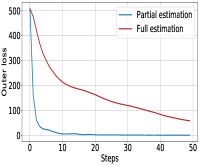
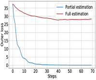
Figure 1: Hyper-representation (HR) with linear (left)/2-layer net (right) embedding model.

However, as demonstrated in Figure 1 (also see our further experiments in Section 4), we empirically observe that such full hypergradient estimation can encounter a large variance and inferior performance, whereas a new zeroth-order-like method PZOBO with partial hypergradient estimation (as we propose below) performs significantly better.

• Encouraged by such an interesting observation, we propose a simple but effective Hessian-free method named PZOBO, which stands for partial zeroth-order-like bilevel optimizer. PZOBO uses a zeroth-order-like approach to approximate only the response Jacobian $\frac{\partial y^{*}(x)}{\partial x}$ (which is the major computational bottleneck of hypergradient) based on the difference between two gradient-based optimization paths. The remaining terms in hypergradient can simply be calculated by their analytical forms. In this way, PZOBO avoids the large variance of the zeroth-order method for estimating the entire hypergradient, but still enjoys its Hessian-free advantage. We further show that PZOBO admits an easy extension to the large-scale stochastic setting by simply taking small-batch gradients without introducing any complex sub-procedure such as the Neumann Series (NS) type of construction in Ji (2021). Experimentally, PZOBO and its stochastic version PZOBO-S achieve superior performance compared to the current baseline bilevel optimizers, and such an improvement is robust across various bilevel problems. In particular, on the few-shot meta-learning problem over a ResNet-12 network, PZOBO outperforms the state-of-the-art optimization-based meta learners (not necessarily bilevel optimizers), while other bilevel optimizers do not scale to solve such meta-learning problems within a comparable time frame.

Furthermore, our zeroth-order-like response Jacobian estimator in PZOBO takes the difference between two optimization-based trajectories, whereas the vanilla zeroth-order method uses the function value difference at two close points for the approximation. Such difference complicates the analysis of PZOBO from three perspectives. (a) Conventional zeroth-order analysis often requires some Lipshitzness properties (e.g., smoothness) of the objective function, whereas they may not hold for the optimization-based output of our response Jacobian estimator. (b) It is unclear if the trajectory-based Hypergradient estimator has bounded error at each iteration, which is critical in the convergence rate analysis for bilevel optimization Ghadimi & Wang (2018); Ji (2021); Hong et al. (2020)). (c) Such characterizations are more challenging for stochastic settings because the randomness along the entire trajectory needs to be considered.

• Theoretically, we provide the convergence rate guarantee for both PZOBO and PZOBO-S. To the best of our knowledge, this is the first known non-asymptotic performance guarantee for Hessian-free bilevel algorithms via zeroth-order-like approximation. Technically, in contrast to the conventional analysis of the zeroth-order estimation on the smoothed blackbox function values, we develop tools to characterize the bias, variance, smoothness and boundedness of the proposed response Jacobian estimator via a recursive analysis over the gradient-based optimization path, which can be of independent interest for zeroth-order estimation based bilevel optimization.

1.1 Related Work

Bilevel optimization. Bilevel optimization has been studied for decades since Bracken & McGill (1973). A variety of bilevel optimization algorithms were then developed, including constraint-based approaches (Hansen et al., 1992; Shi et al., 2005; Moore, 2010), approximate implicit differentiation (AID) approaches (Domke, 2012; Pedregosa, 2016; Gould et al., 2016; Liao et al., 2018; Lorraine et al., 2020) and iterative differentiation (ITD) approaches (Domke, 2012; Maclaurin et al., 2015; Franceschi et al., 2017; Finn et al., 2017; Shaban et al., 2019; Rajeswaran et al., 2019; Liu et al., 2020a). These methods often suffer from expensive computations of second-order information (e.g., Hessian-vector products). Hessian-free algorithms were recently proposed based on interior-point method Liu et al. (2021b) and zeroth-order approximation Gu et al. (2021); Song et al. (2019). Liu et al. (2021c) proposed an initialization auxiliary method to deal with nonconvex inner problem. This paper proposes a more efficient Hessian-free approach via exploiting the benign structure of the hypergradient and a zeroth-order-like response Jacobian estimation. Recently, the convergence rate has been established for gradient-based (Hessian involved) bilevel algorithms (Grazzi et al., 2020; Ji et al., 2021; Rajeswaran et al., 2019; Ji & Liang, 2021). This paper provides a new convergence analysis for the proposed zeroth-order-like bilevel approach.

Stochastic bilevel optimization. Ghadimi & Wang (2018); Ji et al. (2021); Hong et al. (2020) proposed stochastic gradient descent (SGD) type bilevel optimization algorithms by employing Neumann Series for Hessian-inverse-vector approximation. Recent works (Khanduri et al., 2021a, b; Chen et al., 2021; Guo et al., 2021; Guo & Yang, 2021; Yang et al., 2021) then leveraged momentum-based variance reduction to further reduce the computational complexity of existing SGD-type bilevel optimizers from $\mathcal{O}(\epsilon^{-2})$ to $\mathcal{O}(\epsilon^{-1.5})$. In this paper, we propose a stochastic Hessian-free method, which eliminates the computation of second-order information required by all aforementioned stochastic methods.

Bilevel optimization applications. Bilevel optimization has been employed in various applications such as few-shot meta-learning (Snell et al., 2017; Franceschi et al., 2018; Rajeswaran et al., 2019; Zügner & Günnemann, 2019; Ji et al., 2020a, b), hyperparameter optimization (Franceschi et al., 2017; Mackay et al., 2018; Shaban et al., 2019), neural architecture search (Liu et al., 2018a; Zhang et al., 2021), etc. For example, Mackay et al. (2018) models the response function itself as a neural network (where each layer involves an affine transformation of hyperparameters) using the Self-Tuning Networks (STNs). An improved and more stable version of STNs was further proposed in Bae & Grosse (2020), which focused on accurately approximating the response Jacobian rather than the response function itself. This paper demonstrates the superior performance of the proposed Hessian-free bilevel optimizer with guaranteed performance in meta-learning and hyperparameter optimization.

Zeroth-order methods and applications. Zeroth-order optimization methods have been studied for a long time. For example, Nesterov & Spokoiny (2017) proposed an effective zeroth-order gradient estimator via Gaussian smoothing, which was further extended to the stochastic setting by Ghadimi & Lan (2013). Such a technique has exhibited great effectiveness in various applications including meta-reinforcement learning (Song et al., 2019), hyperparameter optimization (Gu et al., 2021), adversarial machine learning (Ji et al., 2019; Liu et al., 2018b), minimax optimization (Liu et al., 2020b; Xu et al., 2020), etc. This paper proposes a novel Jacobian estimator for accelerating bilevel optimization based on an idea similar to zeroth-order estimation via the difference between two optimization paths.

2 Proposed Algorithms

2.1 Hypergradients

The key step in popular gradient-based bilevel optimizers is the estimation of the hypergradient (i.e., the gradient of the objective with respect to the outer variable $x$), which takes the following form:

$$\nabla\Phi(x)=\nabla_{x}f(x,y^{*}(x))+\mathcal{J}_{*}(x)^{\top}\nabla_{y}f(x,y^{*}(x))$$ (2)

where the Jacobian matrix $\mathcal{J}_{*}(x)=\frac{\partial y^{*}(x)}{\partial x}\in\mathbb{R}^{d\times p}$. Following Lorraine et al. (2020), it can be seen that $\nabla\Phi(x)$ contains two components: the direct gradient $\nabla_{x}f(x,y^{*}(x))$ and the indirect gradient $\mathcal{J}_{*}(x)^{\top}\nabla_{y}f(x,y^{*}(x))$. The direct component can be efficiently computed using the existing automatic differentiation techniques. The indirect component, however, is computationally much more complex, because $\mathcal{J}_{*}(x)$ takes the form of $\mathcal{J}_{*}(x)=-\left[\nabla_{y}^{2}g\left(x,y^{*}(x)\right)\right]^{-1}\nabla_{x}\nabla_{y}g\left(x,y^{*}(x)\right)$ (if $\nabla_{y}^{2}g\left(x,y^{*}(x)\right)$ is invertible), which contains the Hessian inverse and the second-order mixed derivative. Some approaches mitigate the issue by designing Jacobian-vector and Hessian-vector products (Pedregosa, 2016; Franceschi et al., 2017; Grazzi et al., 2020) to replace second-order computations. But the computation is still costly for high-dimensional bilevel problems such as those with neural network variables. We next introduce the zeroth-order approach which is at the core for designing efficient Hessian-free bilevel optimizers.

2.2 Zeroth-Order Approximation

Zeroth-order approximation is a powerful technique to estimate the gradient of a function based on function values, when it is not feasible (such as in black-box problems) or computationally costly to evaluate the gradient. The idea of the zeroth-order method in Nesterov & Spokoiny (2017) is to approximate the gradient of a general black-box function $h:\mathbb{R}^{n}\rightarrow\mathbb{R}$ using the following oracle based only on the function values

$$\widehat{\nabla}h(x;u)=\frac{h(x+\mu u)-h(x)}{\mu}u$$ (3)

where $u\in\mathbb{R}^{n}$ is a Gaussian random vector and $\mu>0$ is the smoothing parameter. Such an oracle can be shown to be an unbiased estimator of the gradient of the smoothed function $\mathbb{E}_{u}\left[h(x+\mu u)\right]$.

2.3 Proposed Bilevel Optimizers

Our key idea is to exploit the analytical structure of the hypergradient in eq. 2, where the derivatives $\nabla_{x}f(x,y^{*}(x))$ and $\nabla_{y}f(x,y^{*}(x))$ can be computed efficiently and accurately, and hence use the zero-order estimator similar to eq. 3 to estimate only the Jacobian $\mathcal{J}_{*}(x)$, which is the major term posing computational difficulty. In this way, our estimation of the hypergradient can be much more accurate and reliable. In particular, our Jacobian estimator contains two ingredients: (i) for a given $x$, apply an algorithm to solve the inner optimization problem and use the output as an approximation of $y^{*}(x)$; for example, the output $y^{N}(x)$ of $N$ gradient descent steps of the inner problem can serve as an estimate for $y^{*}(x)$. Then $\mathcal{J}_{N}(x)=\frac{\partial y^{N}(x)}{\partial x}$ serves as an estimate of $\mathcal{J}_{*}(x)$; and (ii) construct the zeroth-order-like Jacobian estimator $\hat{\mathcal{J}}_{N}\left(x;u\right)\in R^{d\times p}$ for $\mathcal{J}_{N}(x)$ as

$$\hat{\mathcal{J}}_{N}\left(x;u\right)=\frac{y^{N}(x+\mu u)-y^{N}(x)}{\mu}u^{\top}$$ (4)

where $u\in\mathbb{R}^{p}$ is a Gaussian vector with independent and identically distributed (i.i.d.) entries. Then for any vector $v\in\mathbb{R}^{d}$, the Jacobian-vector product can be efficiently computed using only vector-vector dot product ${\hat{\mathcal{J}}}_{N}(x;u)^{\top}v=\left\langle\delta(x;u),v\right\rangle u$, where $\delta(x;u)=\frac{y^{N}(x+\mu u)-y^{N}(x)}{\mu}\in\mathbb{R}^{d}$.

Algorithm 1 Partial Zeroth-Order-like Bilevel Optimizer (PZOBO)

1:  Input: lower- and upper-level stepsizes $\alpha,\beta>0$, initializations $x_{0}\in\mathbb{R}^{p}$ and $y_{0}\in\mathbb{R}^{d}$, inner and outer iterations numbers $K$ and $N$, and number of Gaussian vectors $Q$.

2:  for $k=0,1,2,...,K$ do

3:     Set $y^{0}_{k}=y_{0},\;y^{0}_{k,j}=y_{0},\;j=1,...,Q$

4:     for $t=1,2,...,N$ do

5:        Update $y^{t}_{k}=y^{t-1}_{k}-\alpha\nabla_{y}g(x_{k},y^{t-1}_{k})$

6:     end for

7:     for $j=1,...,Q$ do

8:        Generate $u_{k,j}=\mathcal{N}(0,I)\in\mathbb{R}^{p}$

9:        for $t=1,2,...,N$ do

10:           Update $y^{t}_{k,j}=y^{t-1}_{k,j}-\alpha\nabla_{y}g\big{(}x_{k}+\mu u_{k,j},y^{t-1}_{k,j}\big{)}$

11:        end for

12:        Compute $\delta_{j}=\frac{y^{N}_{k,j}-y^{N}_{k}}{\mu}$

13:     end for

14:     Compute $\widehat{\nabla}\Phi(x_{k})=\nabla_{x}f(x_{k},y^{N}_{k})+\frac{1}{Q}\sum_{j=1}^{Q}\left\langle\delta_{j},\nabla_{y}f(x_{k},y^{N}_{k})\right\rangle u_{k,j}$

15:     Update $x_{k+1}=x_{k}-\beta\widehat{\nabla}\Phi(x_{k})$

16:  end for

PZOBO: partial zeroth-order based bilevel optimizer. For the bilevel problem in eq. 1, we design an optimizer (see Algorithm 1) using the Jacobian estimator in eq. 4, which we call as the PZOBO algorithm. Clearly, the zeroth-order estimator is used only for estimating partial hypergradient. At each step $k$ of the algorithm, PZOBO runs an $N$-step full GD to approximate $y_{k}^{N}(x_{k})$. PZOBO then samples $Q$ Gaussian vectors $\{u_{k,j}\in\mathcal{N}(0,I),j=1,...,Q\}$, and for each sample $u_{k,j}$, runs an $N$-step full GD to approximate $y_{k}^{N}(x_{k}+\mu u_{k,j})$, and then computes the Jacobian estimator $\hat{\mathcal{J}}_{N}(x;u_{k,j})$ as in eq. 4. Then the sample average over the $Q$ estimators is used for constructing the following hypergradient estimator for updating the outer variable $x$.

$$\textstyle\widehat{\nabla}\Phi(x_{k}) \textstyle=\nabla_{x}f(x_{k},y^{N}_{k})+\frac{1}{Q}\sum_{j=1}^{Q}\hat{\mathcal{J}}^{T}_{N}(x_{k};u_{k,j})\nabla_{y}f(x_{k},y^{N}_{k})$$

$$\textstyle=\nabla_{x}f(x_{k},y^{N}_{k})+\frac{1}{Q}\sum_{j=1}^{Q}\left\langle\delta(x_{k};u_{k,j}),\nabla_{y}f(x_{k},y^{N}_{k})\right\rangle u_{k,j}.$$ (5)

In our experiments (see Section 4), we choose a small constant-level $Q=\mathcal{O}(1)$ (e.g., $Q=1$ in most applications with neural nets) due to a much better performance. Our convergence guarantee holds for this case, as shown later.

Computationally, in contrast to the existing AID and ITD bilevel optimizers Pedregosa (2016); Franceschi et al. (2018); Grazzi et al. (2020) that contains the complex Hessian- and/or Jacobian-vector product computations, PZOBO has only gradient computations and becomes Hessian-free, and hence is much more efficient as shown in our experiments.

PZOBO-S: stochastic PZOBO. In machine learning applications, the loss functions $f,g$ in eq. 1 often take finite-sum forms over given data ${\mathcal{D}}_{n,m}=\{\xi_{i},\zeta_{j},i=1,...,n,j=1,...,m\}$ as below.

$$f(x,y) \textstyle=\frac{1}{n}\sum_{i=1}^{n}F(x,y;\xi_{i}),\quad g(x,y)\textstyle=\frac{1}{m}\sum_{i=1}^{m}G(x,y;\zeta_{i})$$ (6)

where the sample sizes $n$ and $m$ are typically very large. For such a large-scale scenario, we design a stochastic PZOBO bilevel optimizer (see Algorithm 2 in Appendix A), which we call as PZOBO-S.

Differently from Algorithm 1, which applies GD updates to find $y^{N}(x_{k})$, PZOBO-S uses $N$ stochastic gradient descent (SGD) steps to find $\{Y_{k}^{N},Y_{k,1}^{N},...,Y_{k,Q}^{N}\}$ to the inner problem, each with the outer variable set to be $x_{k}+\mu u_{k,j}$. Note that all SGD runs follow the same batch sampling path $\{{\mathcal{S}}_{0},...,{\mathcal{S}}_{N-1}\}$. The Jacobian estimator $\hat{\mathcal{J}}_{N}(x_{k};u_{k,j})$ can then be computed as in eq. 4. At the outer level, PZOBO-S samples a new batch ${\mathcal{D}}_{F}$ independently from the inner batches $\{{\mathcal{S}}_{0},...,{\mathcal{S}}_{N-1}\}$ to evaluate the stochastic gradients $\nabla_{x}F(x_{k},Y^{N}_{k};{\mathcal{D}}_{F})$ and $\nabla_{y}F(x_{k},Y^{N}_{k};{\mathcal{D}}_{F})$. The hypergradient $\widehat{\nabla}\Phi(x_{k})$ is then estimated as

$$\textstyle\widehat{\nabla}\Phi(x_{k})=\nabla_{x}F(x_{k},Y^{N}_{k};{\mathcal{D}}_{F})+\frac{1}{Q}\sum_{j=1}^{Q}\left\langle\delta(x_{k};u_{k,j}),\nabla_{y}F(x_{k},Y^{N}_{k};{\mathcal{D}}_{F})\right\rangle u_{k,j}.$$ (7)

3 Main Theroetical Results

3.1 Technical Assumptions

In this paper, we consider the following types of objective functions.

Assumption 1.

The inner function $g(x,y)$ is $\mu_{g}$-strongly convex with respect to $y$ and the outer function $f(x,y)$ is possibly nonconvex w.r.t. $x$. For the finite-sum case, the same assumption holds for functions $G(x,y;\zeta)$ and $F(x,y;\zeta)$

The above assumption on $f,g$ has also been adopted in Ghadimi & Wang (2018); Ji et al. (2021); Yang et al. (2021). In fact, many bilevel machine learning problems satisfy this assumption. For example, in few-shot meta-learning, the task-specific parameters are likely the weights of the last classification layer so that the resulting bilevel problem has a strongly-convex inner problem (Raghu et al., 2019; Liu et al., 2021b).

Assumption 2.

Let $w=(x,y)$. The gradient $\nabla g(w)$ is $L_{g}$-Lipschitz continuous, i.e., for any $w_{1},w_{2},\,\|\nabla g(w_{1})-\nabla g(w_{2})\|\leq L_{g}\|w_{1}-w_{2}\|$; further, the derivatives $\nabla_{y}^{2}g(w)$ and $\nabla_{x}\nabla_{y}g(w)$ are $\rho$- and $\tau$-Lipschitz continuous, i.e, $\|\nabla_{y}^{2}g(w_{1})-\nabla_{y}^{2}g(w_{2})\|_{F}\leq\rho\|w_{1}-w_{2}\|$ and $\|\nabla_{x}\nabla_{y}g(w_{1})-\nabla_{x}\nabla_{y}g(w_{2})\|_{F}\leq\tau\|w_{1}-w_{2}\|$. The same assumptions hold for $G(w;\zeta)$ in the finite-sum case.

Assumption 3.

Let $w=(x,y)$. The objective $f(w)$ and its gradient $\nabla f(w)$ are $M$- and $L_{f}$-Lipschitz continuous, i.e., for any $w_{1},w_{2}$, $\big{|}f(w_{1})-f(w_{2})\big{|}\leq M\big{\|}w_{1}-w_{2}\big{\|},\big{\|}\nabla f(w_{1})-\nabla f(w_{2})\big{\|}\leq L_{f}\big{\|}w_{1}-w_{2}\big{\|},$ which hold for $F(w;\xi)$ in the finite-sum case.

Assumption 4.

For the finite-sum case, the gradient $\nabla G(w;\zeta)$ has bounded variance condition, i.e., $\mathbb{E}_{\zeta}\|\nabla G(w;\zeta)-\nabla g(w)\|^{2}\leq\sigma^{2}$ for some constant $\sigma\geq 0$.

3.2 Convergence Analysis for PZOBO

Differently from the standard zeroth-order analysis for a blackbox function, here we develop new techniques to analyze the zeroth-order-like Jacobian estimator that depends on the entire inner optimization trajectory, which is unique in bilevel optimization. We first establish the following important proposition which characterizes the Lipshitzness property of the approximate Jacobian matrix $\mathcal{J}_{N}(x)=\frac{\partial y^{N}(x)}{\partial x}$.

Proposition 1.

Suppose that Assumptions 1 and 2 hold. Let $L_{\mathcal{J}}=\left(1+\frac{L}{\mu_{g}}\right)\left(\frac{\tau}{\mu_{g}}+\frac{\rho L}{\mu_{g}^{2}}\right)$, with $L=\max\{L_{f},L_{g}\}$. Then, the Jacobian $\mathcal{J}_{N}(x)$ is Lipschitz continuous with constant $L_{\mathcal{J}}$:

$$\big{\|}\mathcal{J}_{N}(x_{1})-\mathcal{J}_{N}(x_{2})\big{\|}_{F}\leq L_{\mathcal{J}}\big{\|}x_{1}-x_{2}\big{\|}\quad\forall x_{1},x_{2}\in\mathbb{R}^{p}.$$

We next show that the variance of hypergradient estimation can be bounded. The characterization of the estimation bias can be found in Lemma 8 in the appendix.

Proposition 2.

Suppose that Assumptions 1, 2, and 3 hold. The hypergradient estimation variance can be upper-bounded as

$$\textstyle\mathbb{E} \big{\|}\widehat{\nabla}\Phi(x_{k})-\nabla\Phi(x_{k})\big{\|}^{2}\leq\mathcal{O}\left((1-\alpha\mu_{g})^{N}+\frac{p}{Q}+\mu^{2}dp^{3}+\frac{\mu^{2}dp^{4}}{Q}\right)$$

where $\mathbb{E}[\cdot]$ is conditioned on $x_{k}$ and taken over the Gaussian vectors $\{u_{k,j}:j=1,...,Q\}$.

Proposition 2 upper bounds the hypergradient estimation variance, which mainly arises due to the estimation variance of the Jacobian matrix $\mathcal{J}_{*}$ by the proposed estimator $\mathcal{J}_{N}$, via three types of variances: (a) the approximation variance between $\mathcal{J}_{N}$ and $\mathcal{J}_{*}$ via inner-loop gradient descent, which decreases exponentially w.r.t. the number $N$ of inner iterations due to the strong convexity of the inner objective; (b) the variance between our estimator and the Jacobian $\mathcal{J}_{\mu}$ of the smoothed output $\mathbb{E}_{u}y^{N}(x_{k}+\mu u)$, which decreases sublinearly w.r.t. the batch size $Q$, and (c) the variance between the Jacobian $\mathcal{J}_{N}$ and $\mathcal{J}_{\mu}$, which can be controlled by the smoothness parameter $\mu$.

By using the smoothness property in Proposition 1 and the upper bound in Proposition 2, we provide the following characterization of the convergence rate for PZOBO.

Theorem 1 (Convergence of PZOBO).

Suppose that Assumptions 1, 2, and 3 hold. Choose the inner- and outer-loop stepsizes respectively as $\alpha\leq\frac{1}{L}$ and $\beta=\mathcal{O}(\frac{1}{\sqrt{K}})$. Further, set $Q=\mathcal{O}(1)$ and $\mu=\mathcal{O}\Big{(}\frac{1}{\sqrt{Kdp^{3}}}\Big{)}$. Then, the iterates $x_{k}$ for $k=0,...,K-1$ of PZOBO satisfy

$$\textstyle\frac{1-\frac{1}{\sqrt{K}}}{K}\sum_{k=0}^{K-1}\mathbb{E}\big{\|}\nabla\Phi(x_{k})\big{\|}^{2}\leq\mathcal{O}\left(\frac{p}{\sqrt{K}}+(1-\alpha\mu_{g})^{N}\right)$$

Theorem 1 shows that the convergence rate of PZOBO is sublinear with respect to the number $K$ of outer iterations due to the nonconvexity of the outer objective, and linear (i.e., exponentially decay) with respect to the number $N$ of inner iterations due to the strong convexity.

Theorem 1 also indicates the following features that ensures the efficiency of the algorithms. (i) The batch size $Q$ of the Jacobian estimator can be chosen as a constant (in particular $Q=1$ as in our experiments) so that the computation of the ES estimator is efficient. (ii) The number of inner iterations can be chosen to be small due to its exponential convergence, and hence the algorithm can run efficiently. (iii) PZOBO requires only gradient computations to converge, and eliminates Hessian- and Jacobian-vector products required by the existing AID and ITD based bilevel optimizers (Pedregosa (2016); Franceschi et al. (2018); Grazzi et al. (2020). Thus, PZOBO is more efficient particularly for high-dimensional problems.

3.3 Convergence Analysis for PZOBO-S

In this section, we apply the stochastic algorithm PZOBO-S to the finite-sum objective in eq. 6 and analyze its convergence rate. The following proposition establishes an upper bound on the estimation error of Jacobian $\mathcal{J}_{*}$ by $\mathcal{J}_{N}=\frac{\partial Y^{N}}{\partial x}$, where $Y^{N}$ is the output of $N$ inner SGD updates.

Proposition 3.

Suppose that Assumptions 1, 2, and 4 hold. Choose the inner-loop stepsize as $\alpha=\frac{2}{L+\mu_{g}}$, where $L=\max\{L_{f},L_{g}\}$. Then, we have:

$$\textstyle\mathbb{E}\big{\|}\mathcal{J}_{N}-\mathcal{J}_{*}\big{\|}^{2}_{F}\leq \textstyle C_{\gamma}^{N}\frac{L^{2}}{\mu_{g}^{2}}+\frac{\Gamma}{1-C_{\gamma}}+\frac{\lambda(L+\mu_{g})^{2}(1-\alpha\mu_{g})C_{\gamma}^{N-1}}{(L+\mu_{g})^{2}(1-\alpha\mu_{g})-(L-\mu_{g})^{2}},$$

where $\lambda$, $\Gamma$, and $C_{\gamma}<1$ are constants (see Appendix F for their precise forms).

We next show that the variance of hypergradient estimation is bounded.

Proposition 4.

Suppose that Assumptions 1, 2, 3, and 4 hold. Set the inner-loop stepsize as $\alpha=\frac{2}{L+\mu_{g}}$ where $L=\max\{L_{f},L_{g}\}$. Then, we have:

$$\textstyle\mathbb{E}\big{\|}\widehat{\nabla}\Phi(x_{k})-\nabla\Phi(x_{k})\big{\|}^{2}\leq\mathcal{O}\left((1-\alpha\mu_{g})^{N}+\frac{1}{S}+\frac{1}{D_{f}}+\frac{p}{Q}+\mu^{2}dp^{3}+\frac{\mu^{2}dp^{4}}{Q}\right)$$

where $S$ and $D_{f}$ are the sizes of the inner and outer mini-batches, respectively.

Based on Propositions 1, 3, and 4, we characterize the convergence rate for PZOBO-S.

Theorem 2 (Convergence of PZOBO-S).

Suppose that Assumptions 1, 2, 3, and 4 hold. Set the inner- and outer-loop stepsizes respectively as $\alpha=\frac{2}{L+\mu_{g}}$ and $\beta=\mathcal{O}(\frac{1}{\sqrt{K}})$, where $L=\max\{L_{f},L_{g}\}$. Further, set $Q=\mathcal{O}(1)$, $D_{f}=\mathcal{O}(1)$, and $\mu=\mathcal{O}\Big{(}\frac{1}{\sqrt{Kdp^{3}}}\Big{)}$. Then, the iterates $x_{k},k=0,...,K-1$ of PZOBO-S satisfy:

$$\textstyle\frac{1-\frac{1}{\sqrt{K}}}{K}\sum_{k=0}^{K-1} \textstyle\mathbb{E}\big{\|}\nabla\Phi(x_{k})\big{\|}^{2}\leq\mathcal{O}\left(\frac{p}{\sqrt{K}}+(1-\alpha\mu_{g})^{N}+\frac{1}{\sqrt{S}}\right).$$

Comparing to the convergence bound in Theorem 1 for the deterministic algorithm PZOBO, Theorem 2 for the stochastic algorithm PZOBO-S captures one more sublinearly decreasing error term $\frac{1}{\sqrt{S}}$ due to the sampling of inner batches to estimate the objectives. Note that the sampling of outer batches has been included into the sublinear decay term w.r.t. the number $K$ of outer-loop iterations.

4 Experiments

We validate our algorithms in four bilevel problems: shallow hyper-representation (HR) with linear/2-layer net embedding model on synthetic data, deep HR with LeNet network (LeCun et al., 1998) on MNIST dataset, few-shot meta-learning with ResNet-12 on miniImageNet dataset, and hyperparameter optimization (HO) on the 20 Newsgroup dataset. We run all models using a single NVIDIA Tesla P100 GPU. All running time are in seconds.

(a) $d=128$	(b) $d=256$	(c) PZOBO-N: N inner steps
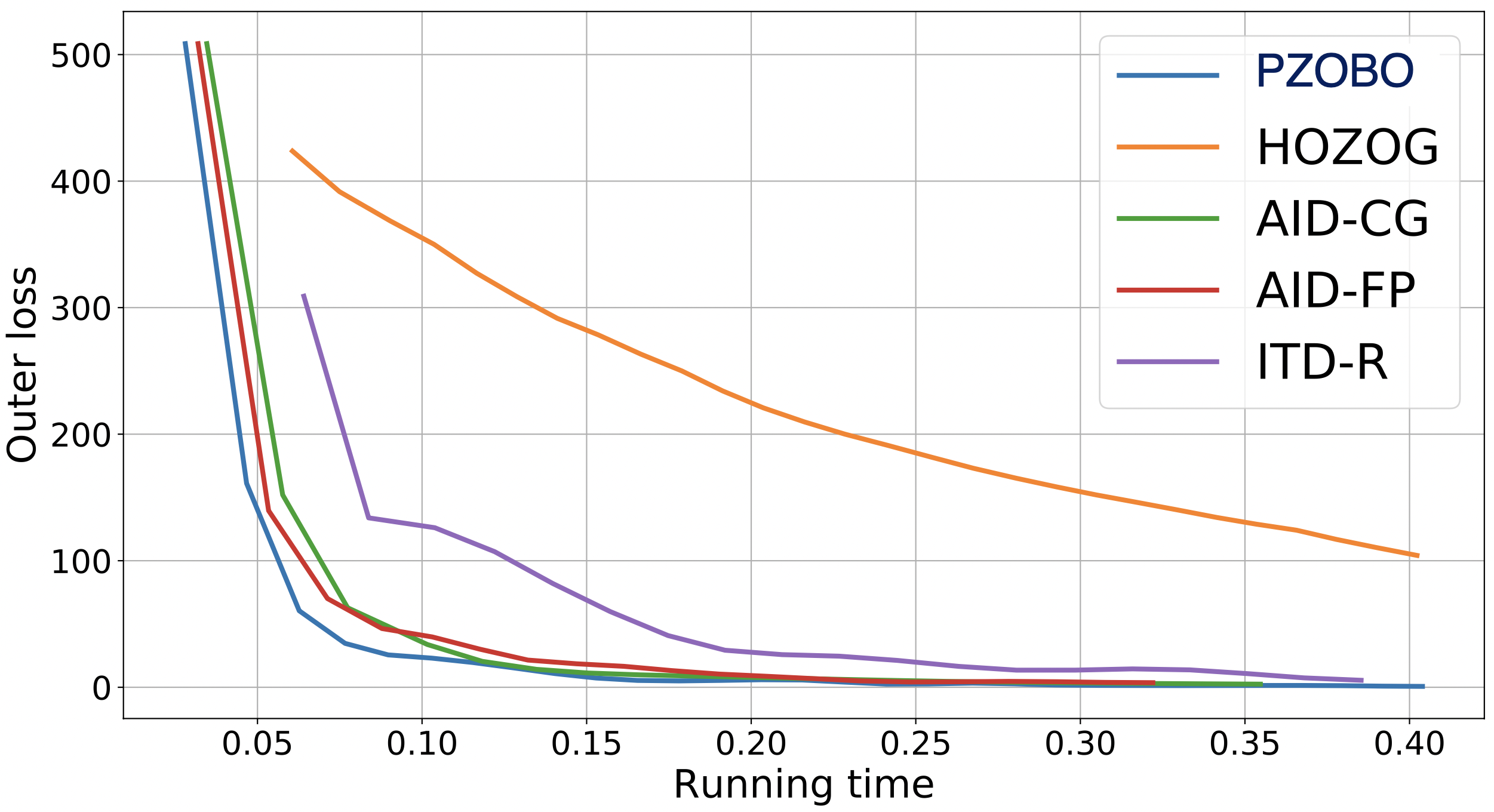
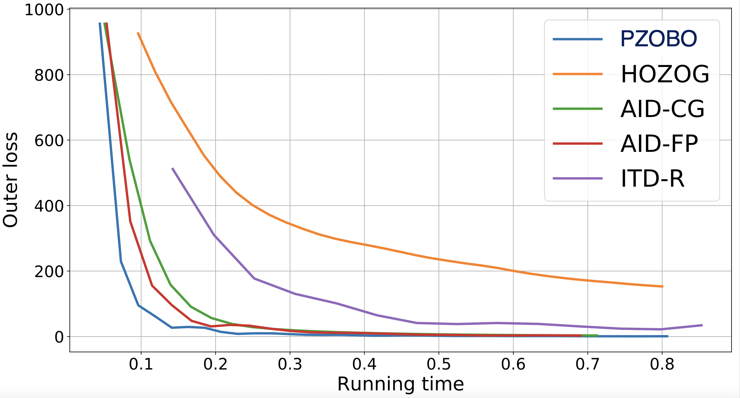
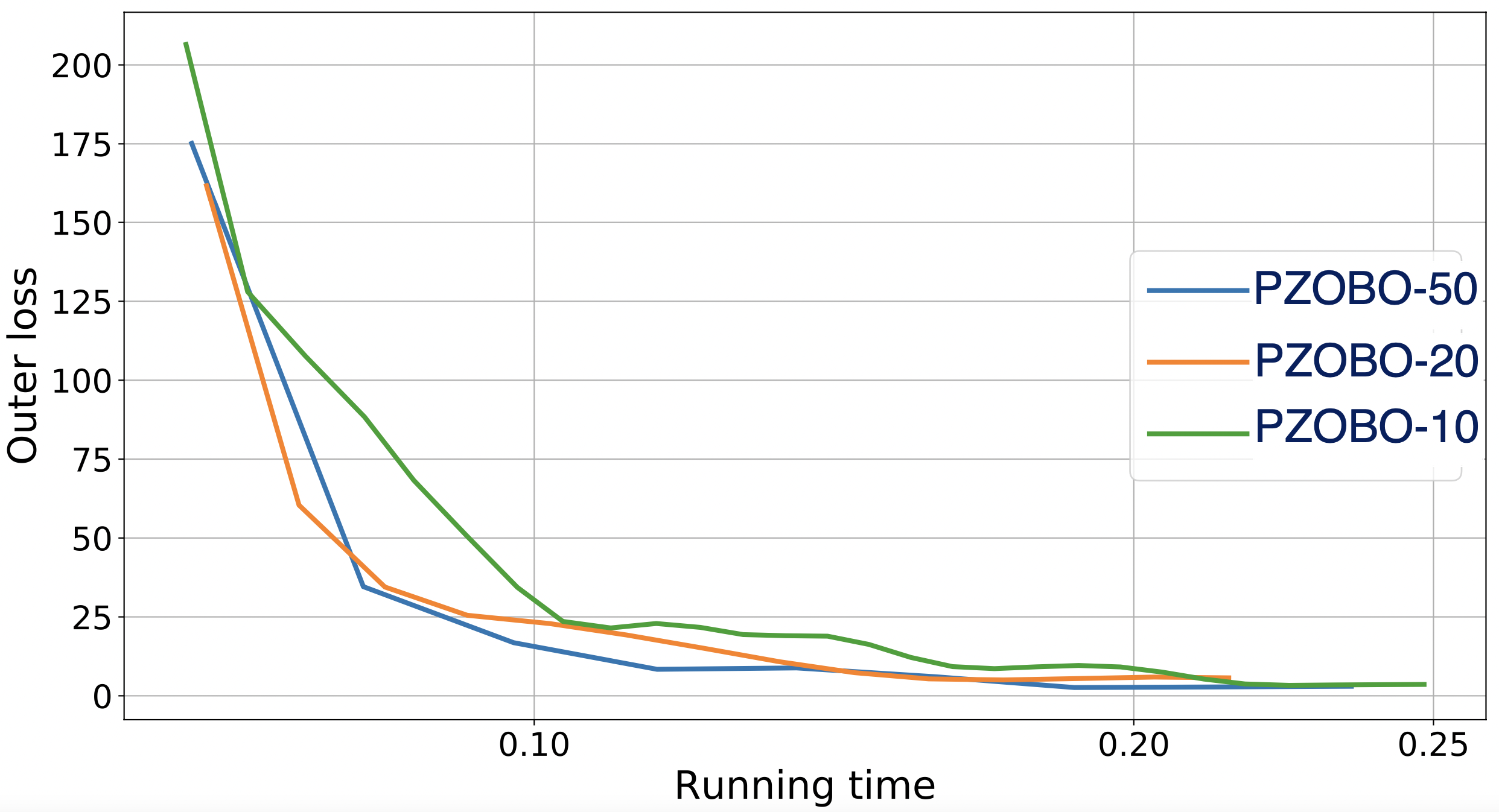
(d) Outer loss	(e) Hypergradient norm	(f) PZOBO-N: N inner steps

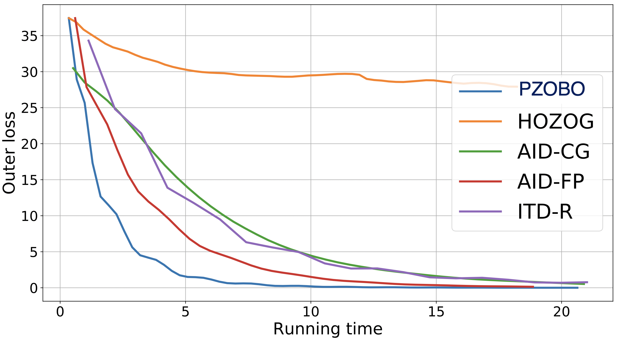
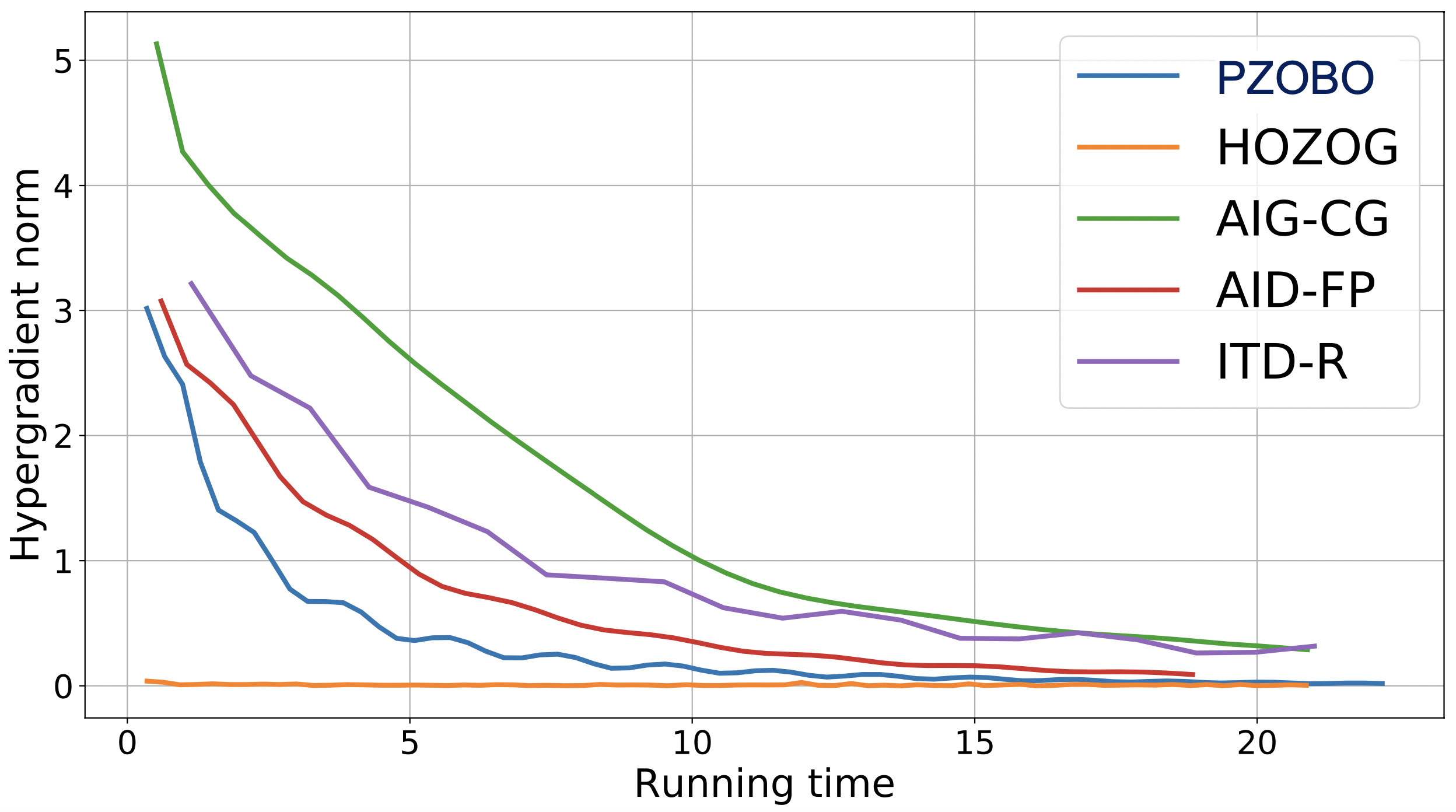
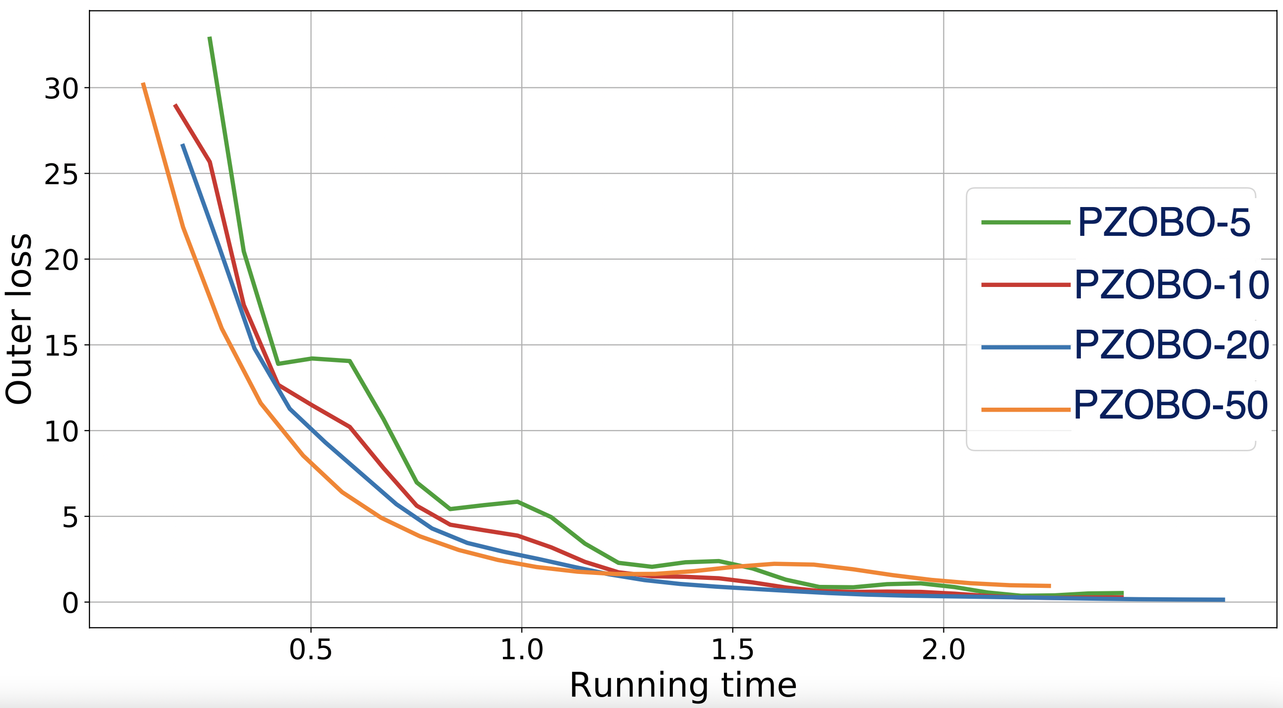
Figure 2: First row: HR with linear embedding model. Second row: HR with two-layer net.

4.1 Shallow Hyper-Representation on Synthetic Data

The hyper-representation (HR) problem (Franceschi et al., 2018; Grazzi et al., 2020) searches for a regression (or classification) model following a two-phased optimization process. The inner-level identifies the optimal linear regressor parameters $w$, and the outer level solves for the optimal embedding model (i.e., representation) parameters $\lambda$. Mathematically, the problem can be modeled by the following bilevel optimization:

$$\min_{\lambda\in\mathbb{R}^{p}}f(\lambda)=\frac{1}{2n_{1}}\left\|T(X_{1};\lambda)w^{*}-Y_{1}\right\|^{2},\text{s.t.}\;w^{*}=\underset{w\in\mathbb{R}^{d}}{\operatorname{argmin}}\frac{1}{2n_{2}}\|T(X_{2};\lambda)w-Y_{2}\|^{2}+\frac{\gamma}{2}\|w\|^{2}$$ (8)

where $X_{2}\in\mathbb{R}^{n_{2}\times m}$ and $X_{1}\in\mathbb{R}^{n_{1}\times m}$ are matrices of synthesized training and validation data, and $Y_{2}\in\mathbb{R}^{n_{2}}$, $Y_{1}\in\mathbb{R}^{n_{1}}$ are the corresponding response vectors. In the case of shallow HR, the embedding function $T(\cdot;\lambda)$ is either a linear transformation or a two-layer network. We generate data matrices $X_{1},X_{2}$ and labels $Y_{1},Y_{1}$ following the same process in Grazzi et al. (2020).

We compare our PZOBO algorithm with the baseline bilevel optimizers AID-FP, AID-CG, ITD-R, and HOZOG (see Section B.1 for details about the baseline algorithms and hyperparameters used). Figure 2 show the performance comparison among the algorithms under linear and two-layer net embedding models. It can be observed that for both cases, our proposed method PZOBO converges faster than all the other approaches, and the advantage of PZOBO becomes more significant in Figure 2 (d), which is under a higher-dimensional model of a two-layer net. In particular, PZOBO outperforms the existing ES-based algorithm HOZOG. This is because HOZOG uses the ES technique to approximate the entire hypergradient, which likely incurs a large estimation error. In contrast, our PZOBO exploits the structure of the hypergradient and only estimate the response Jacobian so that the estimation of hypergradient is more accurate. Such an advantage is more evident under a two-layer net model, where HOZOG does not converge as shown in Figure 2 (d). This can be explained by the flat hypergradient norm as shown in Figure 2 (e), which indicates that the hypergradient estimator in HOZOG fails to provide a good descent direction for the outer optimizer. Figure 2 (c) and (f) further show that the convergence of PZOBO does not change substantially with the number $N$ of inner GD steps, and hence tuning of $N$ in practice is not costly.

4.2 Deep Hyper-Representation on MNIST Dataset

In order to demonstrate the advantage of our proposed algorithms in neural net models, we perform deep hyper-representation to classify MNIST images by learning an entire LeNet network.The problem formulation is described in Section B.3.

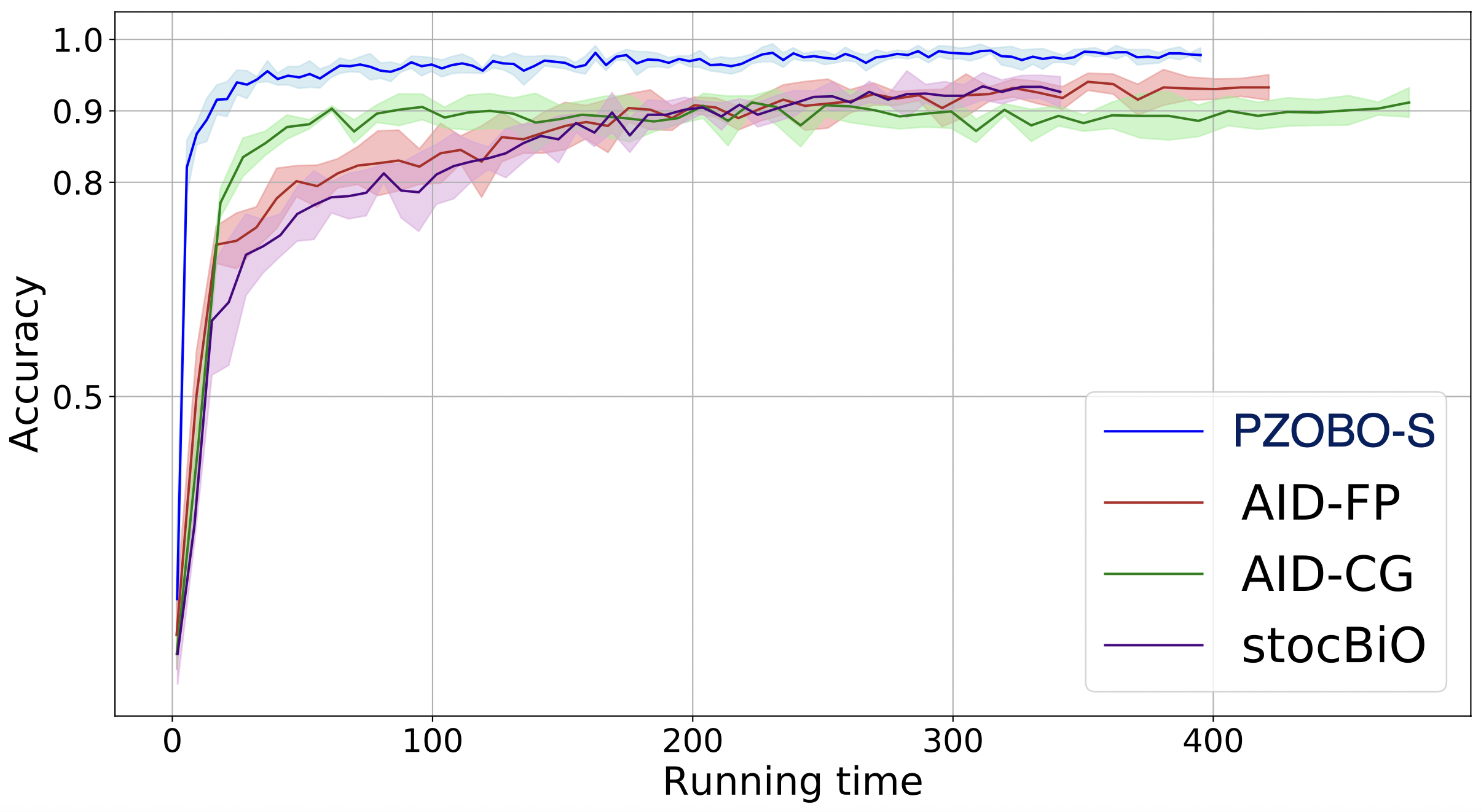
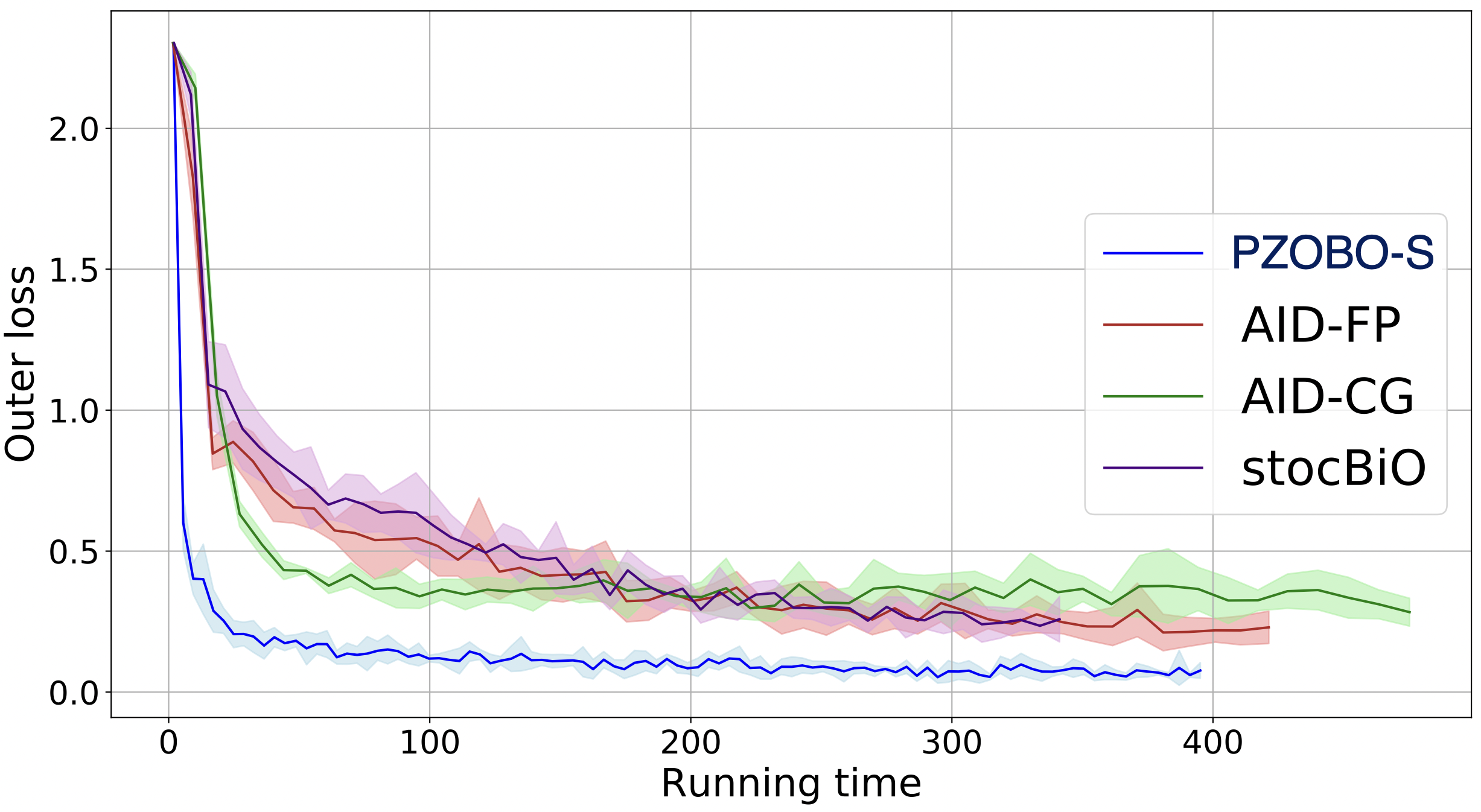
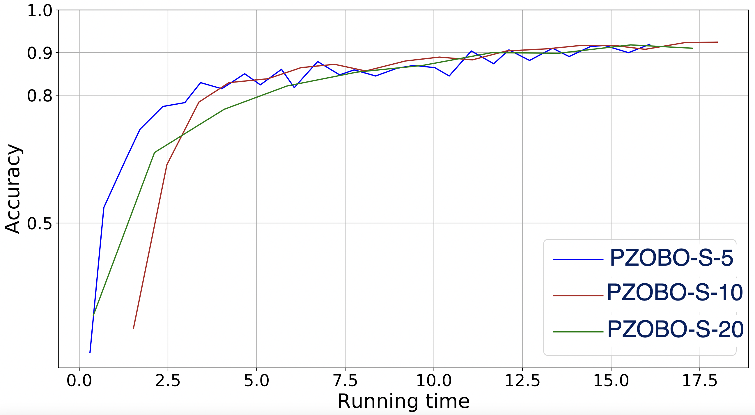
(a) Accuracy on outer data	(b) Outer loss value	(c) PZOBO-S-N: N inner steps

Figure 3: Deep HR on the MNIST dataset.

Figure 3 compares the classification accuracy on the outer dataset $\mathcal{D}_{\mathrm{out}}$ between our PZOBO-S and other stochastic baseline bilevel optimizers including two AID-based stochastic algorithms AID-FP and AID-CG, and a recently proposed new stochastic bilevel optimizer stocBiO which has been demonstrated to exhibit superior performance. Note that ITD and HOZOG are not included in the comparison, because there have not been stochastic algorithms proposed based on these approaches in the literature yet. Our algorithm PZOBO-S converges with the fastest rate and attains the best accuracy with the lowest variance among all algorithms. Note that PZOBO-S is the only bilevel method that is able to attain the same accuracy of $0.98$+ obtained by the state-of-the-art training of all parameters with one-phased optimization on the MNIST dataset using the same backbone network. All other bilevel methods fail to recover such a level of performance, but instead saturate around an accuracy of $0.93$. Further, Figure 3(c) indicates that the convergence of PZOBO-S does not change substantially with the number $N$ of inner SGD steps. This demonstrates the robustness of our method when applied to complex function geometries such as deep nets.

4.3 Few-Shot Meta-Learning over MiniImageNet

We study the few-shot image recognition problem, where classification tasks ${\mathcal{T}}_{i},i=1,...,m$ are sampled over a distribution ${\mathcal{P}}_{\mathcal{T}}$. In particular, we consider the following commonly adopted meta-learning setting (e.g., (Raghu et al., 2019), where all tasks share common embedding features parameterized by $\phi$, and each task ${\mathcal{T}}_{i}$ has its task-specific parameter $w_{i}$ for $i=1,...,m$. More specifically, we set $\phi$ to be the parameters of the convolutional part of a deep CNN model (e.g., ResNet-12 network) and $w$ includes the parameters of the last classification layer. All model parameters ($\phi$, $w$) are trained following a bilevel procedure. In the inner-loop, the base learner of each task ${\mathcal{T}}_{i}$ fixes $\phi$ and minimizes its loss function over a training set ${\mathcal{S}}_{i}$ to obtain its adapted parameters $w_{i}^{*}$. At the outer stage, the meta-learner computes the test loss for each task ${\mathcal{T}}_{i}$ using the parameters ($\phi$, $w_{i}^{*}$) over a test set ${\mathcal{D}}_{i}$, and optimizes the parameters $\phi$ of the common embedding function by minimizing the meta-objective $\mathcal{L}_{\mathrm{meta}}$ over all classification tasks. The detailed problem formulation is given in Section B.4.

We conduct few-shot meta-learning on the miniImageNet dataset (Vinyals et al., 2016) using two different backbone networks for feature extraction: ResNet-12 and CNN4 (Vinyals et al., 2016). The dataset and hyperparameter details can be found in Section B.4. We compare our algorithm PZOBO with four baseline methods for few-shot meta-learning MAML (Finn et al., 2017), ANIL (Raghu et al., 2019), MetaOptNet (Lee et al., 2019), and ProtoNet (Snell et al., 2017). Other bilevel optimizers are not included into comparison because they do not solve the problem within a comparable time frame. Zeroth-order ES-MAML Song et al. (2019) is not included because it exhibits large variance and cannot reach a desired accuracy. Also note that since ProtoNet and MetaOptNet are usually presented in the ResNet setting, and are not relevant in smaller scale networks, we include them into comparison only for our ResNet-12 experiment. We run their efficient Pytorch Lightning implementations available at the learn2learn repository (Arnold et al., 2019).

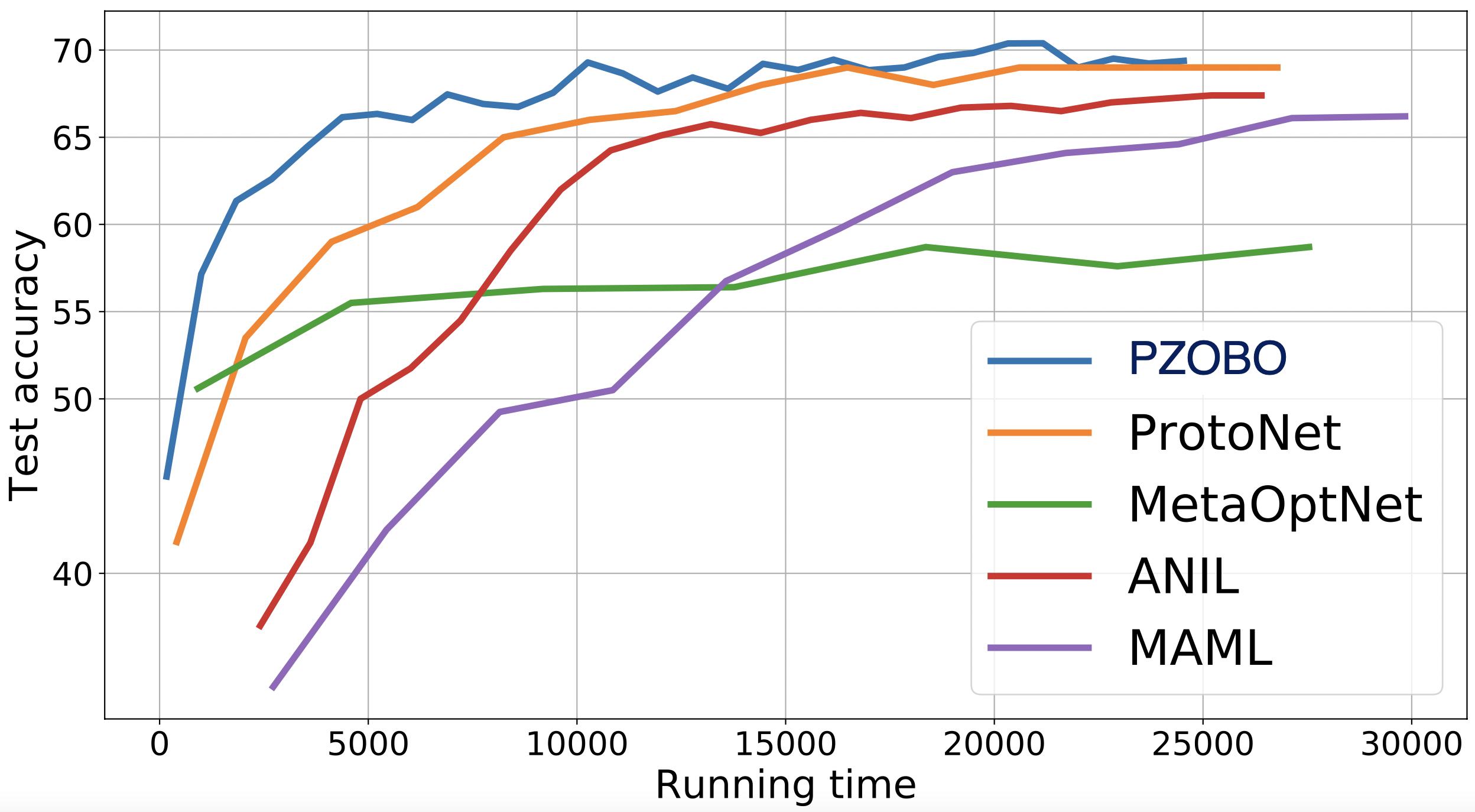
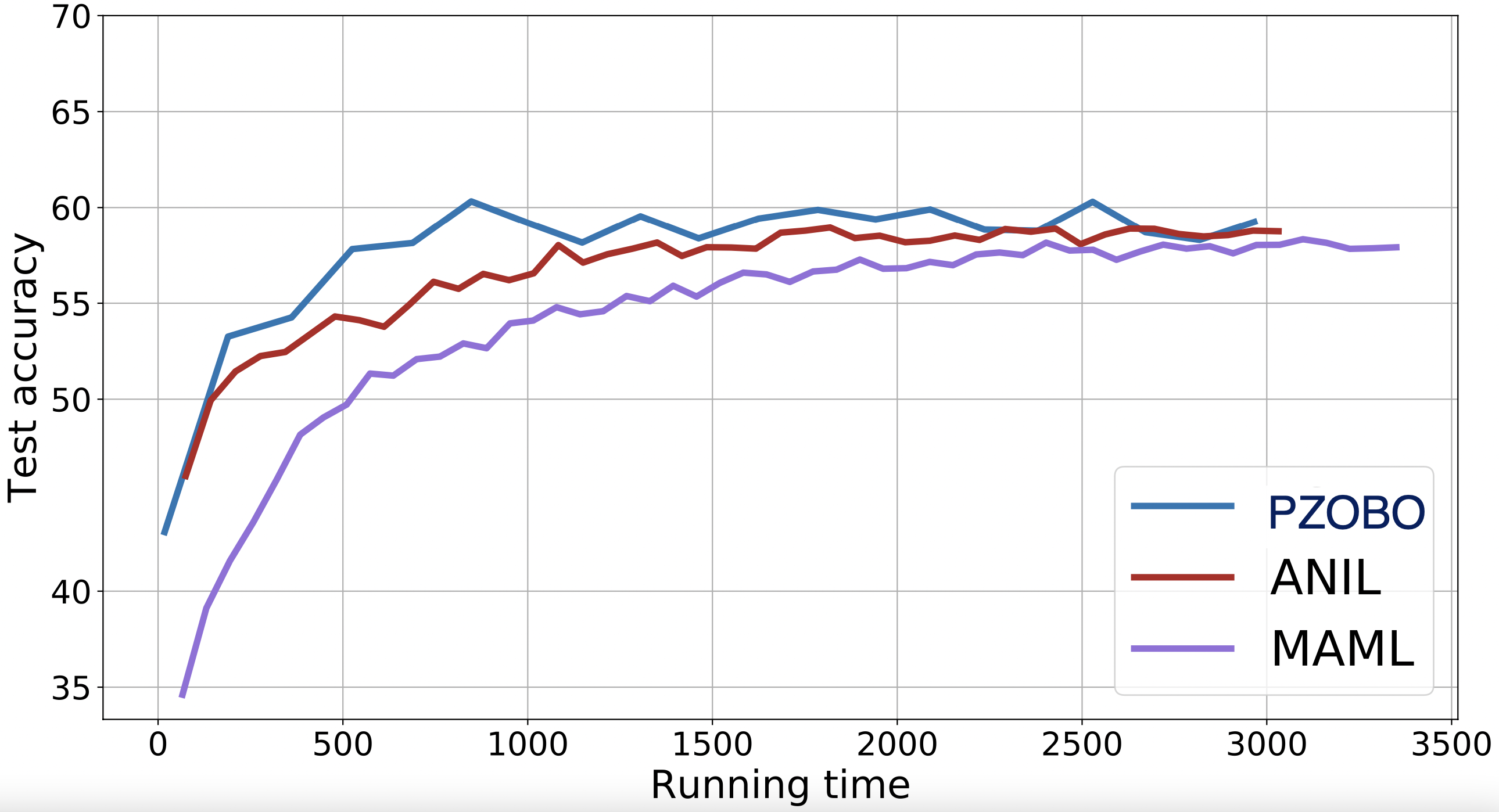
Figure 4: 5way-5shot few-shot classification on the miniImageNet dataset on single GPU. Left plot: Test accuracy (ResNet-12); Right plot: Test accuracy (CNN4)

Algorithm	67%	69%
PZOBO	2.0	2.8
MetaOptNet	20+	20+
ProtNet	3.5	4.4
ANIL	6.3	-
MAML	9.7	-

Table 1: Time (hours) to reach X% accuracy (ResNet-12).

Figure 4(a) and (b) show that our algorithm PZOBO converges faster than the other baseline meta-learning methods. Also, Comparing Figure 4(a) and (b), the advantage of our method over the baselines MAML and ANIL becomes more significant as the size of the network increases. Further, Table 1) shows that MetaOptNet did not reach 69% accuracy after 20 hours of training with ResNet-12 network. In comparison, our PZOBO is able to attain 69% in less than three hours, which is about 1.5 times less than the time taken for ProtoNet to reach the same performance level. Both PZOBO and ProtoNet saturate around 70% accuracy after 10 hours of training.

4.4 Hyperparameter Optimization

Hyperparameter optimization (HO) is the problem of finding the set of the best hyperparamters (either representational or regularization parameters) that yield the optimal value of some criterion of model quality (usually a validation loss on unseen data). HO can be posed as a bilevel optimization problem in which the inner problem corresponds to finding the model parameters by minimizing a training loss (usually regularized) for the given hyperparameters and then the outer problem minimizes over the hyperparameters. We provide a more complete description of the problem and settings in Appendix C.

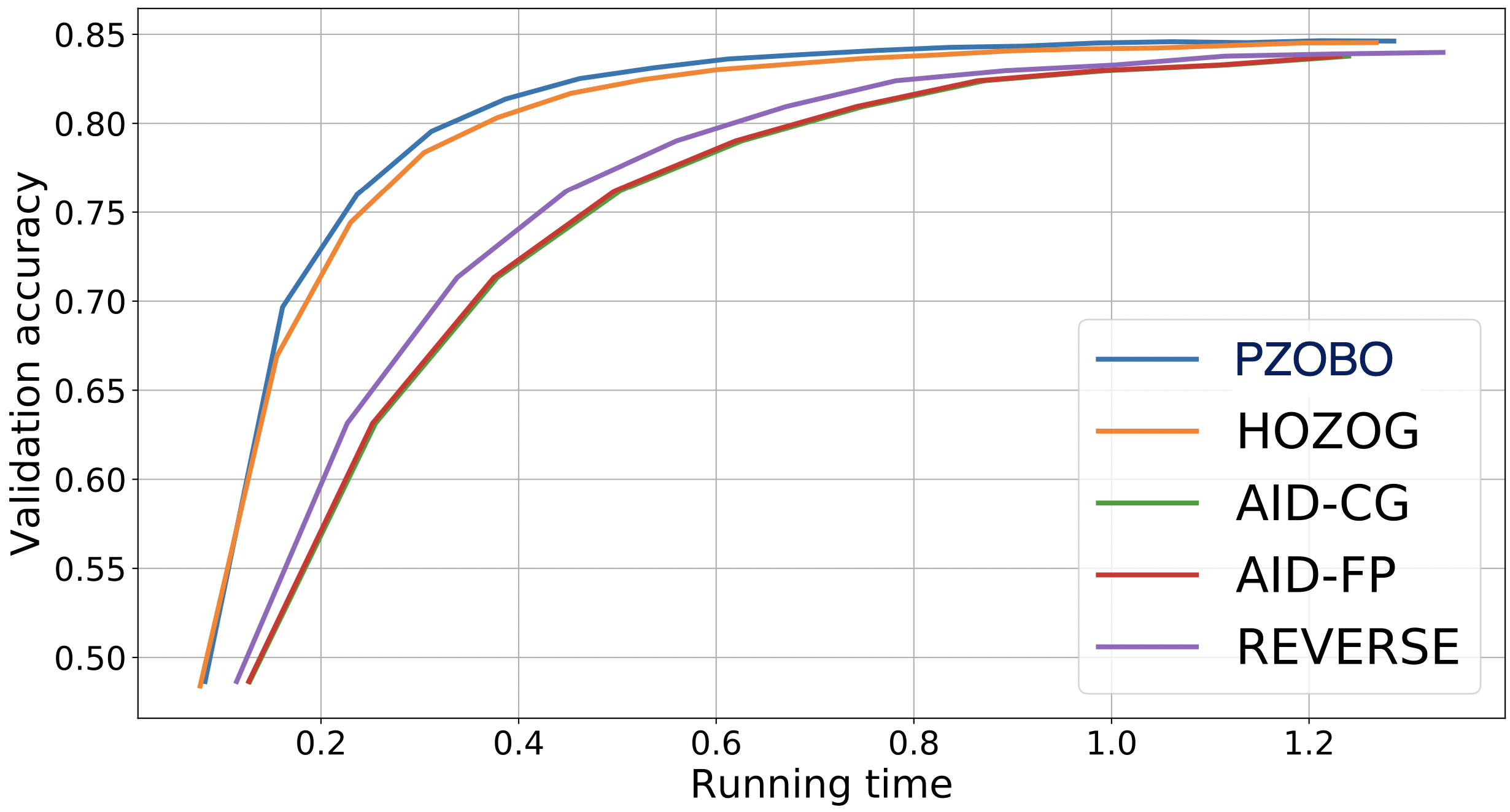
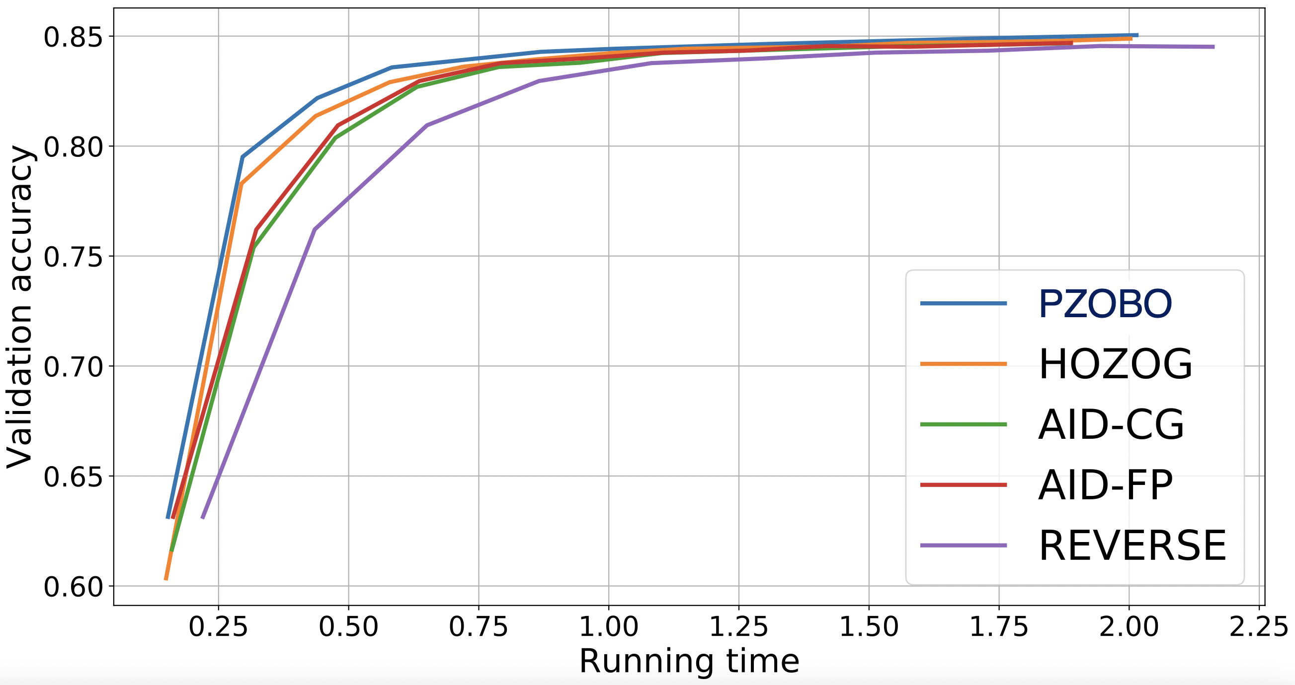
Figure 5: Classification results on 20 Newsgroup dataset. Left: number of inner GD step $N=5$. Right: number of inner GD steps $N=10$.

It can be seen from Figure 5, our method PZOBO slightly outperforms HOZOG and converges faster than the other AID and ITD based approaches. We note that the similar performance for PZOBO and HOZOG can be explained by the fact that in HO, the hypergradient expession in section 2.3 contains only the second term (the first term is zero), which is very close to the approximation in HOZOG method. However, as we have seen in the HR experiments in Figure 2, PZOBO achieves a much better performance than HOZOG. Thus, compared to HOZOG, our PZOBO is much more stable and achieves superior performance across many bilevel problems.

5 Conclusion

In this paper, we propose a novel Hessian-free approach for bilevel optimization based on a zeroth-order-like Jacobian estimator. Compared to the existing such types of Hessian-free algorithms, our approach explores the analytical structure of the hypergradient, and hence leads to much more efficient and accurate hypergradient estimation. Thus, our algorithm outperforms existing baselines in various experiments, particularly in high-dimensional problems. We also provide the convergence guarantee and characterize the convergence rate for our proposed algorithms. We anticipate that our approach and analysis will be useful for bilevel optimization and various machine learning applications.

Supplementary Material

Appendix A Stochastic Bilevel Optimizer PZOBO-S

We present the algorithm specification for our proposed stochastic bilevel optimizer PZOBO-S.

Algorithm 2 Stochastic PZOBO algorithm (PZOBO-S)

1:  Input: lower- and upper-level stepsizes $\alpha,\beta>0$, initializations $x_{0}\in\mathbb{R}^{p}$ and $y_{0}\in\mathbb{R}^{d}$, inner and outer iterations numbers $K$ and $N$, and number of Gaussian vectors $Q$.

2:  for $k=0,1,...,K$ do

3:     Set $Y^{0}_{k}=y_{0},\quad Y^{0}_{k,j}=y_{0},j=1,...,Q$

4:     Generate $u_{k,j}=\mathcal{N}(0,I)\in\mathbb{R}^{p},\quad j=1,...,Q$

5:     for $t=1,2,...,N$ do

6:        Draw a sample batch ${\mathcal{S}}_{t-1}$

7:        Update $Y^{t}_{k}=Y^{t-1}_{k}-\alpha\nabla_{y}G(x_{k},Y^{t-1}_{k};{\mathcal{S}}_{t-1})$

8:        for $j=1,...,Q$ do

9:           Update $Y^{t}_{k,j}=Y^{t-1}_{k,j}-\alpha\nabla_{y}G\left(x_{k}+\mu u_{k,j},Y^{t-1}_{k,j};{\mathcal{S}}_{t-1}\right)$

10:        end for

11:     end for

12:     Compute $\delta_{j}=\frac{Y^{N}_{k,j}-Y^{N}_{k}}{\mu},\quad j=1,...,Q$

13:     Draw a sample batch ${\mathcal{D}}_{F}$

14:     Compute $\widehat{\nabla}\Phi(x_{k})=\nabla_{x}F(x_{k},Y^{N}_{k};{\mathcal{D}}_{F})+\frac{1}{Q}\sum_{j=1}^{Q}\left\langle\delta_{j},\nabla_{y}F(x_{k},Y^{N}_{k};{\mathcal{D}}_{F})\right\rangle u_{k,j}$

15:     Update $x_{k+1}=x_{k}-\beta\widehat{\nabla}\Phi(x_{k})$

16:  end for

Appendix B Further Specifications for Experiments in Section 4

We note that the smoothing parameter $\mu$ (in Algorithms 1 and 2) was easy to set and a value of $0.1$ or $0.01$ yields a good starting point across all our experiments. The batch size $Q$ (in Algorithms 1 and 2) is fixed to $1$ (i.e., we use one Jacobian oracle) in all our experiments.

B.1 Specifications on Baseline Bilevel Approaches in Section 4.1

We compare our algorithm PZOBO with the following baseline methods:

• HOZOG (Gu et al., 2021): a hyperparameter optimization algorithm that uses evolution strategies to estimate the entire hypergradient (both the direct and indirect component). We use our own implementation for this method.

• AID-CG (Grazzi et al., 2020; Rajeswaran et al., 2019): approximate implicit differentiation with conjugate gradient. We use its implementation provided at https://github.com/prolearner/hypertorch

• AID-FP (Grazzi et al., 2020): approximate implicit differentiation with fixed-point. We experimented with its implementation at the repositery https://github.com/prolearner/hypertorch

• ITD-R (REVERSE) (Franceschi et al., 2017): an iterative differentiation method that computes hypergradients using reverse mode automatic differention (RMAD). We use its implementation provided at https://github.com/prolearner/hypertorch.

B.2 Hyperparameters Details for Shallow HR Experiments in Section 4.1

For the linear embedding case, we set the smoothing parameter $\mu$ to be $0.01$ for PZOBO and HOZOG. We use the following hyperparameters for all compared methods. The number of inner GD steps is fixed to $N=20$ with the learning rate of $\alpha=0.001$. For the outer optimizer, we use Adam (Kingma & Ba, 2014) with a learning rate of $0.05$. The value of $\gamma$ in eq. 8 is set to be $0.1$. For the two-layer net case, we use $\mu=0.1$ for PZOBO and HOZOG. For all methods, we set $N=10$, $\alpha=0.001$, $\beta=0.001$, and use Adam with a learning rate of $0.01$ as the outer optimizer.

B.3 Specifications on Problem Formulation and Baseline Stochastic Algorithms in Section 4.2

The corresponding bilevel problem is given by

$$\underset{\lambda}{\min}\hskip 2.0pt\mathcal{L}_{\mathrm{out}}(\lambda):=\frac{1}{\left|\mathcal{D}_{\mathrm{out}}\right|}\underset{(x_{i},y_{i})\in\mathcal{D}_{\mathrm{out}}}{\sum}\mathcal{L}\left(w^{*}(\lambda)f(x_{i};\lambda),y_{i}\right)$$

$$\text{ s.t. }\quad w^{*}(\lambda)=\underset{w\in\mathbb{R}^{c\times p}}{\arg\min}\hskip 2.0pt\mathcal{L}_{\mathrm{in}}(w,\lambda),\quad\mathcal{L}_{\mathrm{in}}(w,\lambda):=\frac{1}{\left|\mathcal{D}_{\mathrm{in}}\right|}\underset{(x_{i},y_{i})\in\mathcal{D}_{\mathrm{in}}}{\sum}\mathcal{L}(wf(x_{i};\lambda),y_{i})+\frac{\beta}{2}\|w\|^{2}$$

where $f(x_{i};\lambda)\in\mathbb{R}^{p}$ corresponds to features extracted from data point $x_{i}$, ${\mathcal{L}}(\cdot,\cdot)$ is the cross-entropy loss function, $c=10$ is the number of categories, and $\mathcal{D}_{\mathrm{in}}$ and $\mathcal{D}_{\mathrm{out}}$ are data used to compute respectively inner and outer loss functions. Since the sizes of $\mathcal{D}_{\mathrm{out}}$ and $\mathcal{D}_{\mathrm{in}}$ are large in the case of MNIST dataset, we apply the more efficient stochastic algorithm PZOBO-S in Algorithm 2 with a minibatch size $B=256$ to estimate the inner and outer losses $\mathcal{L}_{\mathrm{in}}$ and $\mathcal{L}_{\mathrm{out}}$.

We compare our method PZOBO-S to the following baseline stochastic bilevel algorithms.

• stocBiO: an approximate implicit differentiation method that uses Neumann Series to estimate the Hessian inverse. We use its implementation available at https://github.com/JunjieYang97/StocBio.

• AID-CG-S and AID-FP-S: stochastic versions of AID-CG and AID-FP, respectively. We use their implementations in the repository https://github.com/prolearner/hypertorch.

B.4 Specifications for Few-shot Meta-Learning in Section 4.3

Problem formulation. The problem can be expressed as

$$\underset{\phi}{\min}\hskip 2.0pt\mathcal{L}_{\mathrm{meta}}(\phi,\widetilde{w}^{*}):=\frac{1}{m}\sum_{i=1}^{m}\mathcal{L}_{{\mathcal{D}}_{i}}\left(\phi,w_{i}^{*}\right)$$

$$\text{s.t. }\widetilde{w}^{*}=\underset{\widetilde{w}}{\arg\min}\;\mathcal{L}_{\mathrm{adapt}}(\phi,\widetilde{w}):=\frac{1}{m}\sum_{i=1}^{m}\mathcal{L}_{{\mathcal{S}}_{i}}\left(\phi,w_{i}\right),$$ (9)

where we collect all task-specific parameters into $\widetilde{w}=(w_{1},...,w_{m})$ and the corresponding minimizers into $\widetilde{w}^{*}=(w^{*}_{1},...,w^{*}_{m})$. The functions $\mathcal{L}_{{\mathcal{S}}_{i}}\left(\phi,w_{i}\right)=\frac{1}{\left|\mathcal{S}_{i}\right|}\sum_{\zeta\in\mathcal{S}_{i}}(\mathcal{L}(\phi,w_{i};\zeta)+\mathcal{R}(w_{i}))$ and $\mathcal{L}_{{\mathcal{D}}_{i}}\left(\phi,w_{i}^{*}\right)=\frac{1}{\left|\mathcal{D}_{i}\right|}\sum_{\xi\in\mathcal{D}_{i}}\mathcal{L}\left(\phi,w_{i}^{*};\xi\right)$ correspond respectively to the training and test loss functions for task ${\mathcal{T}}_{i}$, with ${\mathcal{R}}$ a strongly-convex regularizer and ${\mathcal{L}}$ a classification loss function. In our setting, since the task-specific parameters correspond to the weights of the last linear layer, the inner-level objective $\mathcal{L}_{\mathrm{adapt}}(\phi,\widetilde{w})$ is strongly convex with respect to $\widetilde{w}=(w_{1},...,w_{m})$. We note that the problem studied in Section 4.2 can be seen as single-task instances of the more general multi-task learning problem in section B.4. However, in contrast to the problem in Section 4.2, the datasets ${\mathcal{D}}_{i}$ and ${\mathcal{S}}_{i}$ are usually small in few-shot learning and full GD can be applied here. Hence, we use ESJ (Algorithm 1) here. Also since the number $m$ of tasks in few-shot classification datasets is often very large, it is preferable to sample a minibatch of i.i.d. tasks by ${\mathcal{P}}_{\mathcal{T}}$ at each meta (i.e., outer) iteration and update the meta parameters based on these tasks.

Experimental setup. The miniImageNet dataset (Vinyals et al., 2016) is a large-scale benchmark for few-shot learning generated from ImageNet (Russakovsky et al., 2015) Russakovsky. The dataset consists of 100 classes with each class containing 600 images of size 84 × 84. Following (Arnold et al., 2019), we split the classes into 64 classes for meta-training, 16 classes for meta-validation, and 20 classes for meta-testing. More specfically, we use 20000 tasks for meta-training, 600 tasks for meta-validation, and 600 tasks for meta-testing. We normalize all image pixels by their means and standard deviations over RGB channels and do not perform any additional data augmentation. At each meta-iteration, we sample a batch of 16 training tasks and update the parameters based on these tasks. We set the smoothness parameter to be $\mu=0.1$ and use $N=30$ inner steps. We use SGD with a learning rate of $\alpha=0.01$ as inner optimizer and Adam with a learning rate of $\beta=0.01$ as outer (meta) optimizer.

Appendix C Experiments on Hyperparameter Optimization

Hyperparameter optimization (HO) is the problem of finding the set of the best hyperparamters (either representational or regularization parameters) that yield the optimal value of some criterion of model quality (usually a validation loss on unseen data). HO can be posed as a bilevel optimization problem in which the inner problem corresponds to finding the model parameters by minimizing a training loss (usually regularized) for the given hyperparameters and then the outer problem minimizes over the hyperparameters. Hence, HO can be mathematically expressed as follows

$$\begin{array}[]{l}\underset{\lambda}{\min}\hskip 2.0pt\mathcal{L}_{\mathrm{val}}(\lambda):=\frac{1}{\left|\mathcal{D}_{\mathrm{val}}\right|}\sum_{\xi\in\mathcal{D}_{\mathrm{val}}}\mathcal{L}\left(w^{*}(\lambda);\xi\right)\\ \text{ s.t. }\quad w^{*}(\lambda)=\underset{w}{\arg\min}\hskip 2.0pt\mathcal{L}_{\mathrm{tr}}(w,\lambda):=\frac{1}{\left|\mathcal{D}_{\mathrm{tr}}\right|}\sum_{\zeta\in\mathcal{D}_{\mathrm{tr}}}(\mathcal{L}(w,\lambda;\zeta)+\mathcal{R}(w,\lambda)),\end{array}$$ (10)

where ${\mathcal{L}}$ is a loss function (e.g., logistic loss), $\mathcal{R}(w,\lambda)$ is a regularizer, and ${\mathcal{D}}_{tr}$ and ${\mathcal{D}}_{val}$ are respectively training and validation data. Note that the loss function used to identify hyperparameters must be different from the one used to find model parameters; otherwise models with higher complexities would be always favored. This is usually achieved in HO by using different data splits (here ${\mathcal{D}}_{val}$ and ${\mathcal{D}}_{tr}$) to compute validation and training losses, and by adding a regularizer term on the training loss.

Figure 6: Classification results on 20 Newsgroup dataset. Left: number of inner GD step $N=5$. Right: number of inner GD steps $N=10$.

Following (Franceschi et al., 2017; Grazzi et al., 2020), we perform classification on the 20 Newsgroup dataset, where the classifier is modeled by an affine transformation, the cost function ${\mathcal{L}}$ is the cross-entrpy loss, and $\mathcal{R}(w,\lambda)$ is a strongly-convex regularizer. We set one $l_{2}$-regularization hyperparameter for each weight in $w$, so that $\lambda$ and $w$ have the same size.

For PZOBO and HOZOG, we use GD with a learning rate of $100$ and a momentum of $0.9$ to perform the inner updates. The outer learning rate is set to be $0.02$. We set the smoothing parameter ($\mu$ in Algorithm 1) to be $0.01$. For AID-FP, AID-CG, and REVERSE we use the suggested hyperparameters in their implementations accompanying the paper Grazzi et al. (2020).

It can be seen from Figure 6, our method PZOBO slightly outperforms HOZOG and converges faster than the other AID and ITD based approaches. We note that the similar performance for PZOBO and HOZOG can be explained by the fact that in HO, the hypergradient expression in section 2.3 contains only the second term (the first term is zero), which is very close to the approximation in HOZOG method. However, as we have seen in the other experiments (not for HO), PZOBO is a more robust and stable bilevel optimizer than HOZOG, and it achieves good performance across many bilevel problems.

Appendix D Supporting Technical Lemmas

In this section, we provide auxiliary lemmas that are used for proving the convergence results for the algorithms PZOBO and PZOBO-S.

In the following proofs, we let $L=\max\{L_{g},L_{f}\}$ and $D$ be such that $\|y^{*}(x)\|\leq D$.

First we recall that for any two matrices $A\in\mathbb{R}^{m\times r}$ and $B\in\mathbb{R}^{r\times n}$, we have the following upper-bound on the Frobenius norm of their product,

$$\big{\|}AB\big{\|}_{F}\leq\big{\|}A\big{\|}\big{\|}B\big{\|}_{F}.$$ (11)

The following lemma follows directly from the Lipschitz properties in Assumptions 2 and 3.

Lemma 1.

Suppose that Assumptions 2 and 3 hold. Then, the stochastic derivatives $\nabla F(x,y;\xi)$, $\nabla_{x}\nabla_{y}G(x,y;\xi)$, and $\nabla_{y}^{2}G(x,y;\xi)$ have bounded variances, i.e., for any $(x,y)$ and $\xi$ we have:

• $\mathbb{E}_{\xi}\big{\|}\nabla F(x,y;\xi)-\nabla f(x,y)\big{\|}^{2}\leq M^{2}$;

• $\mathbb{E}_{\xi}\big{\|}\nabla_{x}\nabla_{y}G(x,y;\xi)-\nabla_{x}\nabla_{y}g(x,y)\big{\|}_{F}^{2}\leq L^{2}$;

• $\mathbb{E}_{\xi}\big{\|}\nabla_{y}^{2}G(x,y;\xi)-\nabla_{y}^{2}g(x,y)\big{\|}_{F}^{2}\leq L^{2}$.

Using Lemma 2.2 in Ghadimi & Wang (2018), the following lemma characterizes the Lipschitz property of the gradient of the total objective $\Phi(x)=f(x,y^{*}(x))$.

Lemma 2.

Suppose that Assumptions 1, 2, and 3 hold. Then, we have:

$$\big{\|}\nabla\Phi(x_{2})-\nabla\Phi(x_{1})\big{\|}\leq L_{\Phi}\big{\|}x_{2}-x_{1}\big{\|}\qquad\forall x_{1}\in\mathbb{R}^{p},x_{2}\in\mathbb{R}^{p},$$

where the constant $L_{\Phi}=L+\frac{2L^{2}+\tau M^{2}}{\mu_{g}}+\frac{\rho LM+L^{3}+\tau ML}{\mu_{g}^{2}}+\frac{\rho L^{2}M}{\mu_{g}^{3}}$.

We next provide some essential properties of the zeroth-order gradient oracle in eq. 3, due to Nesterov & Spokoiny (2017).

Lemma 3.

Let $h:\mathbb{R}^{n}\rightarrow\mathbb{R}$ be a differentiable function with $L$-Lipsctitz gradient. Define its Gaussian smooth approximation $h_{\mu}(x)=\mathbb{E}_{u}\left[h(x+\mu u)\right]$, where $\mu>0$ and $u\in\mathbb{R}^{n}$ is a standard Gaussian random vector. Then, $h_{\mu}$ is differentiable and we have:

• The gradient of $h_{\mu}$ takes the form

  $$\nabla h_{\mu}(x)=\mathbb{E}_{u}\frac{h(x+\mu u)-h(x)}{\mu}u.$$

• For any $x\in\mathbb{R}^{n}$,

  $$\big{\|}\nabla h_{\mu}(x)-\nabla h(x)\big{\|}\leq\frac{\mu}{2}L(n+3)^{3/2}.$$

• For any $x\in\mathbb{R}^{n}$,

  $$\mathbb{E}_{u}\Big{\|}\frac{h(x+\mu u)-h(x)}{\mu}u\Big{\|}^{2}\leq 4(n+4)\big{\|}\nabla h_{\mu}(x)\big{\|}^{2}+\frac{3}{2}\mu^{2}L^{2}(n+5)^{3}.$$

Note the first item in Lemma 3 implies that the oracle in eq. 3 is in indeed an unbiased estimator of the gradient of the smoothed function $h_{\mu}$.

Lemma 4.

Suppose that Assumptions 1 and 2 hold. The Jacobian $\mathcal{J}_{*}=\frac{\partial y^{*}(x)}{\partial x}$ has bounded norm:

$$\big{\|}\mathcal{J}_{*}\big{\|}_{F}\leq\frac{L}{\mu_{g}}.$$ (12)

Proof of Lemma 4.

From the first order optimality condition of $y^{*}(x)$, we have $\nabla_{y}g\left(x,y^{*}(x)\right)=0$. Hence, the Implicit Function Theorem implies:

$$\mathcal{J}_{*}=-\left[\nabla_{y}^{2}g\left(x,y^{*}(x)\right)\right]^{-1}\nabla_{x}\nabla_{y}g\left(x,y^{*}(x)\right).$$ (13)

Taking norms and applying eq. 11 together with Assumptions 1 and 2 yield the desired result

$$\big{\|}\mathcal{J}_{*}\big{\|}_{F}\leq\big{\|}\nabla_{x}\nabla_{y}g\left(x,y^{*}(x)\right)\big{\|}_{F}\big{\|}\left[\nabla_{y}^{2}g\left(x,y^{*}(x)\right)\right]^{-1}\big{\|}\leq\frac{L}{\mu_{g}}.$$ (14)

∎

Lemma 5.

Suppose that Assumptions 1 and 2 hold. The Jacobian $\mathcal{J}_{N}=\frac{\partial y^{N}_{k}}{\partial x_{k}}$ has bounded norm:

$$\big{\|}\mathcal{J}_{N}\big{\|}_{F}\leq\frac{L}{\mu_{g}}.$$ (15)

Proof of Lemma 5.

The inner loop gradient descent updates writes

$$y_{k}^{t}=y_{k}^{t-1}-\alpha\nabla_{y}g\left(x_{k},y_{k}^{t-1}\right),\hskip 10.0ptt=1,\ldots,N.$$

Taking derivatives w.r.t. $x_{k}$ yields

$$\mathcal{J}_{t} =\mathcal{J}_{t-1}-\alpha\nabla_{x}\nabla_{y}g\left(x_{k},y_{k}^{t-1}\right)-\alpha\mathcal{J}_{t-1}\nabla_{y}^{2}g\left(x_{k},y_{k}^{t-1}\right)$$

$$=\mathcal{J}_{t-1}\left(I-\alpha\nabla_{y}^{2}g\left(x_{k},y_{k}^{t-1}\right)\right)-\alpha\nabla_{x}\nabla_{y}g\left(x_{k},y_{k}^{t-1}\right).$$

Telescoping over $t$ from 1 to $N$ yields

$$\mathcal{J}_{N} =\mathcal{J}_{0}\prod_{t=0}^{N-1}\left(I-\alpha\nabla_{y}^{2}g\left(x_{k},y_{k}^{t}\right)\right)-\alpha\sum_{t=0}^{N-1}\nabla_{x}\nabla_{y}g\left(x_{k},y_{k}^{t}\right)\prod_{m=t+1}^{N-1}\left(I-\alpha\nabla_{y}^{2}g\left(x_{k},y_{k}^{m}\right)\right)$$

$$=-\alpha\sum_{t=0}^{N-1}\nabla_{x}\nabla_{y}g\left(x_{k},y_{k}^{t}\right)\prod_{m=t+1}^{N-1}\left(I-\alpha\nabla_{y}^{2}g\left(x_{k},y_{k}^{m}\right)\right).$$ (16)

Hence, we have

$$\big{\|}\mathcal{J}_{N}\big{\|}_{F} \leq\alpha\sum_{t=0}^{N-1}\big{\|}\nabla_{x}\nabla_{y}g\left(x_{k},y_{k}^{t}\right)\big{\|}_{F}\big{\|}\prod_{m=t+1}^{N-1}\left(I-\alpha\nabla_{y}^{2}g\left(x_{k},y_{k}^{m}\right)\right)\big{\|}$$

$$\overset{(i)}{\leq}\alpha\sum_{t=0}^{N-1}L\prod_{m=t+1}^{N-1}\big{\|}I-\alpha\nabla_{y}^{2}g\left(x_{k},y_{k}^{m}\right)\big{\|}$$

$$\overset{(ii)}{\leq}\alpha L\sum_{t=0}^{N-1}(1-\alpha\mu_{g})^{N-1-t}$$

$$=\alpha L\sum_{t=0}^{N-1}(1-\alpha\mu_{g})^{t}\leq\frac{L}{\mu_{g}}$$

where $(i)$ follows from Assumption 2 and $(ii)$ applies the strong-convexity of function $g(x,\cdot)$. This completes the proof. ∎

Lemma 6.

Suppose that Assumptions 1 and 2 hold. Then, the Jacobian $\mathcal{J}_{N}=\frac{\partial Y^{N}_{k}}{\partial x_{k}}$ in the stochastic algorithm PZOBO-S has bounded norm, as shown below.

$$\big{\|}\mathcal{J}_{N}\big{\|}_{F}\leq\frac{L}{\mu_{g}}.$$ (17)

Proof of Lemma 6.

The proof follows similarly to Lemma 5. ∎

D.1 Proof of Proposition 1

Proposition 5 (Restatement of Proposition 1).

Suppose that Assumptions 1 and 2 hold. Define the constant

$$L_{\mathcal{J}}=\left(1+\frac{L}{\mu_{g}}\right)\left(\frac{\tau}{\mu_{g}}+\frac{\rho L}{\mu_{g}^{2}}\right).$$ (18)

Then, the Jacobian $\mathcal{J}_{N}(x)=\frac{\partial y^{N}(x)}{\partial x}$ is $L_{\mathcal{J}}$-Lipschitz with respect to $x$ under the Frobenious norm:

$$\big{\|}\mathcal{J}_{N}(x_{1})-\mathcal{J}_{N}(x_{2})\big{\|}_{F}\leq L_{\mathcal{J}}\big{\|}x_{1}-x_{2}\big{\|}\qquad\forall x_{1}\in\mathbb{R}^{p},x_{2}\in\mathbb{R}^{p}.$$ (19)

Proof of Proposition 1.

Using eq. 16, we have

$$\mathcal{J}_{N}(x)=-\alpha\sum_{t=0}^{N-1}\nabla_{x}\nabla_{y}g\left(x,y^{t}(x)\right)\prod_{m=t+1}^{N-1}\left(I-\alpha\nabla_{y}^{2}g\left(x,y^{m}(x)\right)\right),\hskip 10.0ptx\in\mathbb{R}^{p}.$$

Hence, for $x_{1}\in\mathbb{R}^{p}$ and $x_{2}\in\mathbb{R}^{p}$, we have

$$\big{\|}\mathcal{J}_{N}(x_{1}) -\mathcal{J}_{N}(x_{2})\big{\|}_{F}$$

$$= \alpha\Big{\|}\sum_{t=0}^{N-1}\nabla_{x}\nabla_{y}g\left(x_{1},y^{t}(x_{1})\right)\prod_{m=t+1}^{N-1}\left(I-\alpha\nabla_{y}^{2}g\left(x_{1},y^{m}(x_{1})\right)\right)$$

$$-\sum_{t=0}^{N-1}\nabla_{x}\nabla_{y}g\left(x_{2},y^{t}(x_{2})\right)\prod_{m=t+1}^{N-1}\left(I-\alpha\nabla_{y}^{2}g\left(x_{2},y^{m}(x_{2})\right)\right)\Big{\|}_{F}$$

$$\leq \alpha\sum_{t=0}^{N-1}\big{\|}\nabla_{x}\nabla_{y}g\left(x_{1},y^{t}(x_{1})\right)\prod_{m=t+1}^{N-1}\left(I-\alpha\nabla_{y}^{2}g\left(x_{1},y^{m}(x_{1})\right)\right)$$

$$-\nabla_{x}\nabla_{y}g\left(x_{2},y^{t}(x_{2})\right)\prod_{m=t+1}^{N-1}\left(I-\alpha\nabla_{y}^{2}g\left(x_{2},y^{m}(x_{2})\right)\right)\big{\|}_{F}$$

$$\overset{(i)}{\leq} \alpha\sum_{t=0}^{N-1}\big{\|}\nabla_{x}\nabla_{y}g\left(x_{1},y^{t}(x_{1})\right)\big{\|}_{F}\big{\|}A_{t}(x_{1})-A_{t}(x_{2})\big{\|}$$

$$+\alpha\sum_{t=0}^{N-1}\big{\|}A_{t}(x_{2})\big{\|}\big{\|}\nabla_{x}\nabla_{y}g\left(x_{1},y^{t}(x_{1})\right)-\nabla_{x}\nabla_{y}g\left(x_{2},y^{t}(x_{2})\right)\big{\|}_{F}$$ (20)

where we define $A_{t}(x)=\prod_{m=t+1}^{N-1}\left(I-\alpha\nabla_{y}^{2}g\left(x,y^{m}(x)\right)\right)$ and $(i)$ follows from eq. 11.

Next we upper bound the quantity $\big{\|}A_{t}(x_{1})-A_{t}(x_{2})\big{\|}$, as shown below.

$$\big{\|}A_{t}(x_{1})-A_{t}(x_{2})\big{\|}\leq \big{\|}\alpha\left(\nabla_{y}^{2}g\left(x_{2},y^{t+1}(x_{2})\right)-\nabla_{y}^{2}g\left(x_{2},y^{t+1}(x_{2})\right)\right)A_{t+1}(x_{1})$$

$$+\left(I-\alpha\nabla_{y}^{2}g\left(x_{2},y^{t+1}(x_{2})\right)\right)\left(A_{t+1}(x_{1})-A_{t+1}(x_{2})\right)\big{\|}$$

$$\leq \alpha\big{\|}A_{t+1}(x_{1})\big{\|}\big{\|}\nabla_{y}^{2}g\left(x_{1},y^{t+1}(x_{1})\right)-\nabla_{y}^{2}g\left(x_{2},y^{t+1}(x_{2})\right)\big{\|}$$

$$+\big{\|}I-\alpha\nabla_{y}^{2}g\left(x_{2},y^{t+1}(x_{2})\right)\big{\|}\big{\|}A_{t+1}(x_{1})-A_{t+1}(x_{2})\big{\|}$$

$$\leq (1-\alpha\mu_{g})\big{\|}A_{t+1}(x_{1})-A_{t+1}(x_{2})\big{\|}$$

$$+\alpha\rho(1+\frac{L}{\mu_{g}})(1-\alpha\mu_{g})^{N-t-2}\big{\|}x_{1}-x_{2}\big{\|},$$ (21)

where the last inequality follows from Lemma 5 and Assumptions 1 and 2.

Telescoping eq. 21 over $t$ yields

$$\big{\|}A_{t}(x_{1})-A_{t}(x_{2})\big{\|}\leq (1-\alpha\mu_{g})^{N-t-2}\big{\|}A_{N-2}(x_{1})-A_{N-2}(x_{2})\big{\|}$$

$$+\sum_{m=0}^{N-t-3}\alpha\rho(1+\frac{L}{\mu_{g}})(1-\alpha\mu_{g})^{N-t-2-m}(1-\alpha\mu_{g})^{m}\big{\|}x_{1}-x_{2}\big{\|}$$

$$= (1-\alpha\mu_{g})^{N-t-2}\big{\|}\nabla_{y}^{2}g\left(x_{1},y^{N-1}(x_{1})\right)-\nabla_{y}^{2}g\left(x_{2},y^{N-1}(x_{2})\right)\big{\|}$$

$$+\sum_{m=0}^{N-t-3}\alpha\rho(1+\frac{L}{\mu_{g}})(1-\alpha\mu_{g})^{N-t-2}\big{\|}x_{1}-x_{2}\big{\|}$$

$$\overset{(i)}{\leq} \alpha\rho(1+\frac{L}{\mu_{g}})(1-\alpha\mu_{g})^{N-t-2}\big{\|}x_{1}-x_{2}\big{\|}$$

$$+(N-t-2)\alpha\rho(1+\frac{L}{\mu_{g}})(1-\alpha\mu_{g})^{N-t-2}\big{\|}x_{1}-x_{2}\big{\|}$$

$$= \alpha\rho(1+\frac{L}{\mu_{g}})(N-t-1)(1-\alpha\mu_{g})^{N-t-2}\big{\|}x_{1}-x_{2}\big{\|},$$ (22)

where $(i)$ follows from Lemma 5 and Assumption 2. Replacing eq. 22 in eq. 20 and using Assumption 2, we have

$$\big{\|} \mathcal{J}_{N}(x_{1})-\mathcal{J}_{N}(x_{2})\big{\|}_{F}$$

$$\leq\alpha\sum_{t=0}^{N-1}L\alpha\rho(1+\frac{L}{\mu_{g}})(N-t-1)(1-\alpha\mu_{g})^{N-t-2}\big{\|}x_{1}-x_{2}\big{\|}$$

$$+\alpha\sum_{t=0}^{N-1}\tau(1+\frac{L}{\mu_{g}})(1-\alpha\mu_{g})^{N-t-1}\big{\|}x_{1}-x_{2}\big{\|}$$

$$\leq\alpha^{2}L\rho(1+\frac{L}{\mu_{g}})\big{\|}x_{1}-x_{2}\big{\|}\sum_{m=0}^{N-1}m(1-\alpha\mu_{g})^{m-1}+\frac{\tau}{\mu_{g}}(1+\frac{L}{\mu_{g}})\big{\|}x_{1}-x_{2}\big{\|}$$

$$\leq\frac{\rho L}{\mu_{g}^{2}}(1+\frac{L}{\mu_{g}})\big{\|}x_{1}-x_{2}\big{\|}+\frac{\tau}{\mu_{g}}(1+\frac{L}{\mu_{g}})\big{\|}x_{1}-x_{2}\big{\|}$$ (23)

where we use $\sum_{m=0}^{N-1}mx^{m-1}\leq\frac{1}{\alpha^{2}\mu_{g}^{2}}$ in eq. 23, which can be obtained by taking derivatives for the expression $\sum_{m=0}^{N-1}x^{m}$ with respect to $x$. Hence, rearranging and using the definition of $L_{\mathcal{J}}$ in eq. 18 finishes the proof. ∎

Lemma 7.

Suppose that Assumptions 1 and 2 hold. Define the constant

$$L_{\mathcal{J}}=\left(1+\frac{L}{\mu_{g}}\right)\left(\frac{\tau}{\mu_{g}}+\frac{\rho L}{\mu_{g}^{2}}\right).$$

Then, the Jacobian $\mathcal{J}_{N}(x)=\frac{\partial Y^{N}(x;\cdot)}{\partial x}$ is $L_{\mathcal{J}}$-Lipschitz with respect to $x$ under the Frobenius norm:

$$\big{\|}\mathcal{J}_{N}(x_{1};\cdot)-\mathcal{J}_{N}(x_{2};\cdot)\big{\|}_{F}\leq L_{\mathcal{J}}\big{\|}x_{1}-x_{2}\big{\|}\qquad\forall x_{1}\in\mathbb{R}^{p},x_{2}\in\mathbb{R}^{p}.$$

Proof of Lemma 7.

The proof follows similarly to that for Proposition 1. ∎

Appendix E Proofs for Deterministic Bilevel Optimization

For notation convenience, we define the following quantities:

$$\hat{\mathcal{J}}_{N,j} =\hat{\mathcal{J}}_{N}(x_{k},u_{j})=\left(\begin{array}[]{c}\frac{y^{N}_{1}(x_{k}+\mu u_{j})-y^{N}_{1}(x_{k})}{\mu}u_{j}^{\top}\\ \vdots\\ \frac{y^{N}_{d}(x_{k}+\mu u_{j})-y^{N}_{d}(x_{k})}{\mu}u_{j}^{\top}\end{array}\right),\quad{\mathcal{J}}_{N}=\frac{\partial y^{N}_{k}}{\partial x_{k}},\quad{\mathcal{J}}_{*}=\frac{\partial y^{*}_{k}}{\partial x_{k}},$$ (27)

where $u_{j}\in\mathbb{R}^{p},j=1,\ldots,Q$ are standard Gaussian vectors. Let $y_{i,\mu}^{N}(x_{k})$ be the Gaussian smooth approximation of $y^{N}_{i}(x_{k})$. We collect $y_{i,\mu}^{N}(x_{k})$ for $i=1,\ldots,d$ together as a vector $y_{\mu}^{N}(x_{k})$, which is the Gaussian approximation of the vector $y^{N}(x_{k})$. If $\mu>0$, $y_{\mu}^{N}(x_{k})$ is differentiable and we let $\mathcal{J}_{\mu}$ be the Jocobian given by

$$\mathcal{J}_{\mu}=\frac{\partial y_{\mu}^{N}(x_{k})}{\partial x_{k}}.$$ (28)

We approximate $\frac{\partial y^{N}_{k}}{\partial x_{k}}$ using the average zeroth-order estimator given by $\hat{\mathcal{J}}_{N}=\frac{1}{Q}\sum_{j=1}^{Q}\hat{\mathcal{J}}_{N,j}.$ The hypergradient is then approximated as

$$\widehat{\nabla}\Phi(x_{k}) =\nabla_{x}f(x_{k},y^{N}_{k})+{\hat{\mathcal{J}}}^{\top}_{N}\nabla_{y}f(x_{k},y^{N}_{k})$$

$$=\nabla_{x}f(x_{k},y^{N}_{k})+\frac{1}{Q}\sum_{j=1}^{Q}{\hat{\mathcal{J}}}^{\top}_{N,j}\nabla_{y}f(x_{k},y^{N}_{k}).$$ (29)

Let $\delta_{j}=\frac{y^{N}(x_{k}+\mu u_{j})-y^{N}(x_{k})}{\mu}$ and let $\delta_{i,j}$ be the $i$-th component of $\delta_{j}$. Hence, we have

$$\hat{\mathcal{J}}_{N,j}=\left(\begin{array}[]{c}\delta_{1,j}u_{j}^{\top}\\ \delta_{2,j}u_{j}^{\top}\\ \vdots\\ \delta_{d,j}u_{j}^{\top}\end{array}\right),$$

$${\hat{\mathcal{J}}}^{\top}_{N,j}\nabla_{y}f(x_{k},y^{N}_{k}) =\left(\begin{array}[]{cccc}\delta_{1,j}u_{j}&\delta_{2,j}u_{j}&\ldots&\delta_{d,j}u_{j}\end{array}\right)\nabla_{y}f(x_{k},y^{N}_{k})$$ (31)

$$=\left\langle\delta_{j},\nabla_{y}f(x_{k},y^{N}_{k})\right\rangle u_{j}.$$ (32)

Using eq. 29 and eq. 32, the estimator for the hypergradient can thus be computed as

$$\widehat{\nabla}\Phi(x_{k}) =\nabla_{x}f(x_{k},y^{N}_{k})+\frac{1}{Q}\sum_{j=1}^{Q}\left\langle\delta_{j},\nabla_{y}f(x_{k},y^{N}_{k})\right\rangle u_{j}.$$

E.1 Proof of Proposition 2

Proposition 6 (Formal Statement of Proposition 2).

Suppose that Assumptions 1, 2, and 3 hold. Then, the variance of hypergradient estimation can be upper-bounded as

$$\mathbb{E}\big{\|}\widehat{\nabla}\Phi(x_{k})-\nabla\Phi(x_{k})\big{\|}^{2}\leq 2L^{2}D^{2}(1-\alpha\mu_{g})^{N}+4\frac{L^{4}}{\mu_{g}^{2}}D^{2}(1-\alpha\mu_{g})^{N}+24(4p+15)\frac{L^{2}M^{2}}{Q\mu_{g}^{2}}$$

$$+\frac{\mu^{2}}{Q}L_{\mathcal{J}}^{2}M^{2}d\mathcal{P}_{4}(p)+\frac{24L^{2}M^{2}(1-\alpha\mu_{g})^{2N}}{\mu_{g}^{2}}+6\mu^{2}L_{\mathcal{J}}^{2}M^{2}d(p+3)^{3}$$

$$+\frac{48M^{2}(\tau\mu_{g}+L\rho)^{2}}{\mu_{g}^{4}}(1-\alpha\mu_{g})^{N-1}D^{2}$$

$$= \mathcal{D}_{var}=\mathcal{O}\left((1-\alpha\mu_{g})^{N}+\frac{p}{Q}+\frac{\mu^{2}dp^{4}}{Q}+\mu^{2}dp^{3}\right)$$ (33)

where the expectation $\mathbb{E}[\cdot]$ is conditioned on $x_{k}$ and $y_{k}^{N}$.

Proof of Proposition 2.

Based on the definitions of $\nabla\Phi(x_{k})$ and $\widehat{\nabla}\Phi(x_{k})$ and conditioning on $x_{k}$ and $y_{k}^{N}$, we have

$$\mathbb{E}\big{\|}\widehat{\nabla} \Phi(x_{k})-\nabla\Phi(x_{k})\big{\|}^{2}$$

$$\leq 2\big{\|}\nabla_{x}f(x_{k},y^{N}_{k})-\nabla_{x}f(x_{k},y^{*}_{k})\big{\|}^{2}+2\mathbb{E}\big{\|}{\hat{\mathcal{J}}}^{\top}_{N}\nabla_{y}f(x_{k},y^{N}_{k})-{\mathcal{J}}^{\top}_{*}\nabla_{y}f(x_{k},y^{*}_{k})\big{\|}^{2}$$

$$\leq 2L^{2}\big{\|}y^{N}_{k}-y^{*}_{k}\big{\|}^{2}+4\big{\|}{\mathcal{J}}_{*}\big{\|}_{F}^{2}\big{\|}\nabla_{y}f(x_{k},y^{N}_{k})-\nabla_{y}f(x_{k},y^{*}_{k})\big{\|}^{2}$$

$$+4\mathbb{E}\big{\|}\hat{\mathcal{J}}_{N}-\mathcal{J}_{*}\big{\|}_{F}^{2}\big{\|}\nabla_{y}f(x_{k},y^{N}_{k})\big{\|}^{2}$$

$$\overset{(i)}{\leq} 2L^{2}D^{2}(1-\alpha\mu_{g})^{N}+4\frac{L^{4}}{\mu_{g}^{2}}\big{\|}y^{N}_{k}-y^{*}_{k}\big{\|}^{2}+4M^{2}\mathbb{E}\big{\|}\hat{\mathcal{J}}_{N}-\mathcal{J}_{*}\big{\|}^{2}_{F}$$

$$\overset{(ii)}{\leq} 2L^{2}D^{2}(1-\alpha\mu_{g})^{N}+4\frac{L^{4}}{\mu_{g}^{2}}D^{2}(1-\alpha\mu_{g})^{N}+4M^{2}\mathbb{E}\big{\|}\hat{\mathcal{J}}_{N}-\mathcal{J}_{*}\big{\|}^{2}_{F}$$ (34)

where $(i)$ follows from Lemma 4 and Assumption 3, and $(i)$ and $(ii)$ also use the following result for full GD (when applied to a strongly-convex function).

$$\big{\|}y^{N}_{k}-y^{*}_{k}\big{\|}^{2}\leq(1-\alpha\mu_{g})^{N}D^{2}.$$

Next, we upper-bound the last term $\mathbb{E}\big{\|}\hat{\mathcal{J}}_{N}-\mathcal{J}_{*}\big{\|}^{2}_{F}$ at the last line of eq. 34. First note that

$$\mathbb{E}\big{\|}\hat{\mathcal{J}}_{N}-\mathcal{J}_{*}\big{\|}^{2}_{F}\leq 3\mathbb{E}\big{\|}\hat{\mathcal{J}}_{N}-\mathcal{J}_{\mu}\big{\|}^{2}_{F}+3\big{\|}\mathcal{J}_{N}-\mathcal{J}_{*}\big{\|}^{2}_{F}+3\big{\|}\mathcal{J}_{\mu}-\mathcal{J}_{N}\big{\|}^{2}_{F}.$$ (35)

We then upper-bound each term of the right hand side of eq. 35. For the first term, we have

$$\mathbb{E}\big{\|}\hat{\mathcal{J}}_{N}-\mathcal{J}_{\mu}\big{\|}^{2}_{F}= \mathbb{E}\big{\|}\frac{1}{Q}\sum_{j=1}^{Q}\hat{\mathcal{J}}_{N,j}-\mathcal{J}_{\mu}\big{\|}^{2}_{F}$$

$$= \frac{1}{Q^{2}}\mathbb{E}\big{\|}\sum_{j=1}^{Q}\left(\hat{\mathcal{J}}_{N,j}-\mathcal{J}_{\mu}\right)\big{\|}^{2}_{F}$$

$$= \frac{1}{Q^{2}}\mathbb{E}\left(\sum_{j=1}^{Q}\big{\|}\hat{\mathcal{J}}_{N,j}-\mathcal{J}_{\mu}\big{\|}^{2}_{F}+2\sum_{i<j}\left\langle\hat{\mathcal{J}}_{N,i}-\mathcal{J}_{\mu},\hat{\mathcal{J}}_{N,j}-\mathcal{J}_{\mu}\right\rangle\right)$$

$$= \frac{1}{Q^{2}}\sum_{j=1}^{Q}\mathbb{E}\big{\|}\hat{\mathcal{J}}_{N,j}-\mathcal{J}_{\mu}\big{\|}^{2}_{F}$$

$$= \frac{1}{Q}\mathbb{E}\big{\|}\hat{\mathcal{J}}_{N,j}-\mathcal{J}_{\mu}\big{\|}^{2}_{F},\hskip 10.0ptj\in\{1,\ldots,Q\}.$$ (36)

We next upper-bound the term $\mathbb{E}\big{\|}\hat{\mathcal{J}}_{N,j}-\mathcal{J}_{\mu}\big{\|}^{2}_{F}$ in eq. 36.

$$\mathbb{E}\big{\|}\hat{\mathcal{J}}_{N,j}-\mathcal{J}_{\mu}\big{\|}^{2}_{F}= \mathbb{E}\big{\|}\hat{\mathcal{J}}_{N,j}\big{\|}^{2}_{F}-\big{\|}\mathcal{J}_{\mu}\big{\|}^{2}_{F}$$

$$\overset{(i)}{\leq} \sum_{i=1}^{d}\left(4(p+4)\big{\|}\nabla y^{N}_{i,\mu}\big{\|}^{2}+\frac{3}{2}\mu^{2}L_{\mathcal{J}}^{2}(p+5)^{3}\right)-\sum_{i=1}^{d}\big{\|}\nabla y^{N}_{i,\mu}\big{\|}^{2}$$

$$\leq \sum_{i=1}^{d}\left((4p+15)\big{\|}\nabla y^{N}_{i,\mu}\big{\|}^{2}+\frac{3}{2}\mu^{2}L_{\mathcal{J}}^{2}(p+5)^{3}\right),$$ (37)

where $(i)$ follows by applying Lemma 3 to the components of vector $y^{N}(x_{k})$ which have Lipschitz gradients by Proposition 1. Then, noting that $\big{\|}\nabla y^{N}_{i,\mu}\big{\|}^{2}\leq 2\big{\|}\nabla y^{N}_{i}\big{\|}^{2}+\frac{1}{2}\mu^{2}L_{\mathcal{J}}^{2}(p+3)^{3}$ and replacing in eq. 37, we have

$$\mathbb{E}\big{\|}\hat{\mathcal{J}}_{N,j}-\mathcal{J}_{\mu}\big{\|}^{2}_{F}\leq \sum_{i=1}^{d}\left(2(4p+15)\big{\|}\nabla y^{N}_{i}\big{\|}^{2}+\mu^{2}L_{\mathcal{J}}^{2}\mathcal{P}_{4}(p)\right)$$

$$\leq 2(4p+15)\big{\|}\mathcal{J}_{N}\big{\|}^{2}_{F}+\mu^{2}L_{\mathcal{J}}^{2}d\mathcal{P}_{4}(p)$$

$$\overset{(i)}{\leq} 2(4p+15)\frac{L^{2}}{\mu_{g}^{2}}+\mu^{2}L_{\mathcal{J}}^{2}d\mathcal{P}_{4}(p),$$ (38)

where $(i)$ follows from Lemma 5 and $\mathcal{P}_{4}$ is a polynomial of degree $4$ in $p$. Combining eq. 36 and eq. 37 yields

$$\mathbb{E}\big{\|}\hat{\mathcal{J}}_{N}-\mathcal{J}_{\mu}\big{\|}^{2}_{F}\leq 2(4p+15)\frac{L^{2}}{Q\mu_{g}^{2}}+\frac{\mu^{2}}{Q}L_{\mathcal{J}}^{2}d\mathcal{P}_{4}(p).$$ (39)

We next upper-bound the second term at the right hand side of eq. 35, which can be upper-bounded using eq. (41) in Ji et al. (2021), as shown below.

$$\big{\|}\mathcal{J}_{N}-\mathcal{J}_{*}\big{\|}^{2}\leq\frac{2L^{2}(1-\alpha\mu_{g})^{2N}}{\mu_{g}^{2}}+\frac{4(\tau\mu_{g}+L\rho)^{2}}{\mu_{g}^{4}}(1-\alpha\mu_{g})^{N-1}D^{2}.$$ (40)

We finally upper-bound the last term at the right hand side of eq. 35 using Lemma 3.

$$\big{\|}{\mathcal{J}}_{\mu}-{\mathcal{J}}_{N}\big{\|}^{2}_{F}= \sum_{i=1}^{d}\big{\|}\nabla y_{i,\mu}^{N}-\nabla y_{i}^{N}\big{\|}^{2}$$

$$\leq \frac{\mu^{2}}{2}L_{\mathcal{J}}^{2}d(p+3)^{3}.$$ (41)

Substituting eq. 39, eq. 40 and section E.1 into eq. 35 yields

$$\mathbb{E}\big{\|}\hat{\mathcal{J}}_{N}-\mathcal{J}_{*}\big{\|}^{2}_{F}\leq 6(4p+15)\frac{L^{2}}{Q\mu_{g}^{2}}+\frac{\mu^{2}}{Q}L_{\mathcal{J}}^{2}d\mathcal{P}_{4}(p)+\frac{6L^{2}(1-\alpha\mu_{g})^{2N}}{\mu_{g}^{2}}$$

$$+\frac{12(\tau\mu_{g}+L\rho)^{2}}{\mu_{g}^{4}}(1-\alpha\mu_{g})^{N-1}D^{2}+\frac{3\mu^{2}}{2}L_{\mathcal{J}}^{2}d(p+3)^{3}.$$ (42)

Finally, the bound for the expected estimation error in eq. 34 becomes

$$\mathbb{E}\big{\|}\widehat{\nabla}\Phi(x_{k})-\nabla\Phi(x_{k})\big{\|}^{2}\leq 2L^{2}D^{2}(1-\alpha\mu_{g})^{N}+4\frac{L^{4}}{\mu_{g}^{2}}D^{2}(1-\alpha\mu_{g})^{N}+24(4p+15)\frac{L^{2}M^{2}}{Q\mu_{g}^{2}}$$

$$+\frac{\mu^{2}}{Q}L_{\mathcal{J}}^{2}M^{2}d\mathcal{P}_{4}(p)+\frac{24L^{2}M^{2}(1-\alpha\mu_{g})^{2N}}{\mu_{g}^{2}}+6\mu^{2}L_{\mathcal{J}}^{2}M^{2}d(p+3)^{3}$$

$$+\frac{48M^{2}(\tau\mu_{g}+L\rho)^{2}}{\mu_{g}^{4}}(1-\alpha\mu_{g})^{N-1}D^{2}.$$ (43)

This completes the proof. ∎

E.2 Hypergradient Estimation Bias

Lemma 8.

Suppose that Assumptions 1, 2, and 3 hold. Then, the bias of hypergradient estimation can be upper-bounded as follows:

$$\big{\|}\mathbb{E}\widehat{\nabla}\Phi(x_{k})-\nabla\Phi(x_{k})\big{\|}\leq\mathcal{D}_{bias}=\mathcal{O}\left((1-\alpha\mu_{g})^{N/2}+\mu d^{1/2}p^{3/2}\right).$$ (44)

Proof.

First note that We have

$$\big{\|}\mathbb{E}\widehat{\nabla}\Phi(x_{k}) -\nabla\Phi(x_{k})\big{\|}$$

$$= \big{\|}\nabla_{x}f(x_{k},y^{N}_{k})-\nabla_{x}f(x_{k},y^{*}_{k})\big{\|}+\big{\|}{\mathcal{J}}^{\top}_{\mu}\nabla_{y}f(x_{k},y^{N}_{k})-{\mathcal{J}}^{\top}_{*}\nabla_{y}f(x_{k},y^{*}_{k})\big{\|}$$

$$\leq L\big{\|}y^{N}_{k}-y^{*}_{k}\big{\|}+\big{\|}{\mathcal{J}}^{\top}_{\mu}\nabla_{y}f(x_{k},y^{N}_{k})-{\mathcal{J}}^{\top}_{*}\nabla_{y}f(x_{k},y^{N}_{k})\big{\|}$$

$$+\big{\|}{\mathcal{J}}^{\top}_{*}\nabla_{y}f(x_{k},y^{N}_{k})-{\mathcal{J}}^{\top}_{*}\nabla_{y}f(x_{k},y^{*}_{k})\big{\|}$$

$$\leq L\big{\|}y^{N}_{k}-y^{*}_{k}\big{\|}+M\big{\|}{\mathcal{J}}_{\mu}-{\mathcal{J}}_{*}\big{\|}+\frac{L}{\mu_{g}}\big{\|}\nabla_{y}f(x_{k},y^{N}_{k})-\nabla_{y}f(x_{k},y^{*}_{k})\big{\|}$$

$$\leq L\big{\|}y^{N}_{k}-y^{*}_{k}\big{\|}+M\big{\|}{\mathcal{J}}_{\mu}-{\mathcal{J}}_{*}\big{\|}+\frac{L^{2}}{\mu_{g}}\big{\|}y^{N}_{k}-y^{*}_{k}\big{\|}.$$

which, in conjunction with $\|{\mathcal{J}}_{\mu}-{\mathcal{J}}_{*}\|=\|{\mathcal{J}}_{\mu}-{\mathcal{J}}_{N}\big{\|}+\|{\mathcal{J}}_{N}-{\mathcal{J}}_{*}\|\leq\frac{\mu}{2}L_{\mathcal{J}}d^{1/2}(p+3)^{3/2}+\frac{L(1-\alpha\mu_{g})^{N}}{\mu_{g}}+\frac{2(\tau\mu_{g}+L\rho)}{\mu_{g}^{2}}(1-\alpha\mu_{g})^{(N-1)/2}D$, yields

$$\big{\|}\mathbb{E}\widehat{\nabla}\Phi(x_{k})-\nabla\Phi(x_{k})\big{\|}\leq LD(1-\alpha\mu_{g})^{N/2}+\frac{\mu}{2}L_{\mathcal{J}}Md^{1/2}(p+3)^{3/2}+\frac{LM(1-\alpha\mu_{g})^{N}}{\mu_{g}}$$

$$+\frac{2MD(\tau\mu_{g}+L\rho)}{\mu_{g}^{2}}(1-\alpha\mu_{g})^{(N-1)/2}+\frac{L^{2}D}{\mu_{g}}(1-\alpha\mu_{g})^{N/2}$$

$$\leq \mathcal{O}\left((1-\alpha\mu_{g})^{N/2}+\mu d^{1/2}p^{3/2}\right).$$

Then, the proof is complete. ∎

E.3 Proof of Theorem 1

Theorem 3 (Formal Statement of Theorem 1).

Suppose that Assumptions 1, 2, and 3 hold. Choose the inner- and outer-loop stepsizes respectively as $\alpha\leq\frac{1}{L}$ and $\beta=\frac{1}{L_{\Phi}\sqrt{K}}$, where $L_{\Phi}=L+\frac{2L^{2}+\tau M^{2}}{\mu_{g}}+\frac{\rho LM+L^{3}+\tau ML}{\mu_{g}^{2}}+\frac{\rho L^{2}M}{\mu_{g}^{3}}$, and let $M_{\Phi}=\big{(}1+\frac{L_{g}}{\mu_{g}}\big{)}M$. Further set $Q=\mathcal{O}(1)$ and $\mu=\mathcal{O}\left(\frac{1}{\sqrt{Kdp^{3}}}\right)$. Then, the iterates $x_{k}$ for $k=0,...,K-1$ of PZOBO in Algorithm 1 satisfy:

$$\frac{1-\frac{1}{\sqrt{K}}}{K}\sum_{k=0}^{K-1}\mathbb{E}\big{\|}\nabla\Phi(x_{k})\big{\|}^{2}\leq\frac{L_{\phi}(\Phi(x_{0})-\Phi^{*})}{\sqrt{K}}+M_{\Phi}\mathcal{D}_{bias}+\frac{\mathcal{D}_{var}}{\sqrt{K}}=\mathcal{O}\left(\frac{p}{\sqrt{K}}+(1-\alpha\mu_{g})^{N}\right),$$ (45)

with $\Phi^{*}=\inf_{x}\Phi(x)$, $\mathcal{D}_{bias}$ and $\mathcal{D}_{var}$ are defined in Lemma 8 and Proposition 6.

Proof of Theorem 1.

Using Assumptions 1, 2, and 3, we upper-bound the hypergradient $\nabla\Phi(x_{k})$ by

$$\|\nabla\Phi(x)\|= \|\nabla_{x}f(x,y^{*}(x))-\nabla_{x}\nabla_{y}g\left(x,y^{*}(x)\right)\left[\nabla_{y}^{2}g\left(x,y^{*}(x)\right)\right]^{-1}\nabla_{y}f(x,y^{*}(x))\|$$

$$\leq \Big{(}1+\frac{L_{g}}{\mu_{g}}\Big{)}M.$$ (46)

Then, using the Lipschitzness of function $\Phi(x_{k})$, we have

$$\Phi(x_{k+1})\leq \Phi(x_{k})+\left\langle\nabla\Phi(x_{k}),x_{k+1}-x_{k}\right\rangle+\frac{L_{\phi}}{2}\big{\|}x_{k+1}-x_{k}\big{\|}^{2}$$

$$\leq \Phi(x_{k})-\beta\langle\nabla\Phi(x_{k}),\widehat{\nabla}\Phi(x_{k})\rangle+\frac{L_{\phi}}{2}\beta^{2}\big{\|}\widehat{\nabla}\Phi(x_{k})\big{\|}^{2}$$

$$\leq \Phi(x_{k})-\beta\langle\nabla\Phi(x_{k}),\widehat{\nabla}\Phi(x_{k})-\nabla\Phi(x_{k})\rangle-\beta\big{\|}\nabla\Phi(x_{k})\big{\|}^{2}$$

$$+L_{\phi}\beta^{2}\left(\big{\|}\nabla\Phi(x_{k})\big{\|}^{2}+\big{\|}\widehat{\nabla}\Phi(x_{k})-\nabla\Phi(x_{k})\big{\|}^{2}\right)$$ (47)

Let $\mathbb{E}_{k}[\cdot]=\mathbb{E}_{u_{k,1:Q}}[\cdot|x_{k},y^{N}_{k}]$ be the expectation over the Gaussian vectors $u_{k,1},\ldots,u_{k,Q}$ conditioned on $x_{k}$ and $y_{k}^{N}$. Applying the expectation $\mathbb{E}_{k}[\cdot]$ to section E.3 yields

$$\mathbb{E}_{k}\Phi(x_{k+1})\leq \Phi(x_{k})-\beta\langle\nabla\Phi(x_{k}),\mathbb{E}_{k}\widehat{\nabla}\Phi(x_{k})-\nabla\Phi(x_{k})\rangle-\beta\big{\|}\nabla\Phi(x_{k})\big{\|}^{2}$$

$$+L_{\phi}\beta^{2}\left(\big{\|}\nabla\Phi(x_{k})\big{\|}^{2}+\mathbb{E}_{k}\big{\|}\widehat{\nabla}\Phi(x_{k})-\nabla\Phi(x_{k})\big{\|}^{2}\right)$$

$$\leq \Phi(x_{k})+\beta\big{\|}\nabla\Phi(x_{k})\big{\|}\big{\|}\mathbb{E}_{k}\widehat{\nabla}\Phi(x_{k})-\nabla\Phi(x_{k})\big{\|}-(\beta-L_{\phi}\beta^{2})\big{\|}\nabla\Phi(x_{k})\big{\|}^{2}$$

$$+L_{\phi}\beta^{2}\mathbb{E}_{k}\big{\|}\widehat{\nabla}\Phi(x_{k})-\nabla\Phi(x_{k})\big{\|}^{2}$$

$$\leq \Phi(x_{k})+\beta M_{\Phi}\mathcal{D}_{bias}-(\beta-L_{\phi}\beta^{2})\big{\|}\nabla\Phi(x_{k})\big{\|}^{2}+\beta^{2}L_{\phi}\mathcal{D}_{var}$$ (48)

where $\mathcal{D}_{bias}$ and $\mathcal{D}_{var}$ represent respectively the upper-bound established for for the bias and variance. Now taking total expectation over $\mathcal{U}_{k}=\{u_{1,1:Q},\ldots,u_{k,1:Q}\}$, we have

$$E_{k+1}\leq E_{k}-\beta(1-L_{\phi}\beta)\mathbb{E}_{\mathcal{U}_{k}}\big{\|}\nabla\Phi(x_{k})\big{\|}^{2}+\beta M_{\Phi}\mathcal{D}_{bias}+\beta^{2}L_{\phi}\mathcal{D}_{var}$$ (49)

where $E_{k}=\mathbb{E}_{\mathcal{U}_{k-1}}\Phi(x_{k})$. Summing up the inequalities in eq. 49 for $k=0,\ldots,K-1$ yields

$$E_{K}\leq E_{0}-\beta(1-L_{\phi}\beta)\sum_{k=0}^{K-1}\mathbb{E}_{\mathcal{U}_{k}}\big{\|}\nabla\Phi(x_{k})\big{\|}^{2}+\beta KM_{\Phi}\mathcal{D}_{bias}+\beta^{2}KL_{\phi}\mathcal{D}_{var}$$ (50)

Setting $\beta=\frac{1}{L_{\phi}\sqrt{K}}$, denoting by $\Phi^{*}=\inf_{x}\Phi(x)$, and rearranging eq. 50, we have

$$\frac{1-\frac{1}{\sqrt{K}}}{K}\sum_{k=0}^{K-1}\mathbb{E}_{\mathcal{U}_{k}}\big{\|}\nabla\Phi(x_{k})\big{\|}^{2}\leq\frac{L_{\phi}(\Phi(x_{0})-\Phi^{*})}{\sqrt{K}}+M_{\Phi}\mathcal{D}_{bias}+\frac{\mathcal{D}_{var}}{\sqrt{K}}.$$

Setting $Q=\mathcal{O}(1)$ and $\mu=\mathcal{O}\left(\frac{1}{\sqrt{Kdp^{3}}}\right)$ in the expressions of $\mathcal{D}_{bias}$ and $\mathcal{D}_{var}$ finishes the proof. ∎

Appendix F Proofs for Stochastic Bilevel Optimization

Define the following quantities

$$\hat{\mathcal{J}}_{N,j} =\hat{\mathcal{J}}_{N}\left(x_{k},u_{j}\right)=\left(\begin{array}[]{ccc}\frac{Y^{N}_{1}(x_{k}+\mu u_{j};\mathcal{S})-Y^{N}_{1}(x_{k};\mathcal{S})}{\mu}u_{j}^{\top}\\ \vdots\\ \frac{Y^{N}_{d}(x_{k}+\mu u_{j};\mathcal{S})-Y^{N}_{d}(x_{k};\mathcal{S})}{\mu}u_{j}^{\top}\end{array}\right),\quad{\mathcal{J}}_{N}=\frac{\partial Y^{N}_{k}}{\partial x_{k}},\quad{\mathcal{J}}_{*}=\frac{\partial y^{*}_{k}}{\partial x_{k}}$$

where $u_{j}\in\mathbb{R}^{p},j=1,\ldots,Q$ are standard Gaussian vectors and $Y^{N}_{k}$ is the output of SGD obtained with the minibatches $\{{\mathcal{S}}_{0},...,{\mathcal{S}}_{N-1}\}$.

Conditioning on $x_{k}$ and $Y^{N}_{k}$ and taking expectation over $u_{j}$ yields

$$\mathbb{E}_{u_{j}}\hat{\mathcal{J}}_{N,j} =\mathbb{E}_{u_{j}}\left(\begin{array}[]{ccc}\frac{Y^{N}_{1}(x_{k}+\mu u_{j};\mathcal{S})-Y^{N}_{1}(x_{k};\mathcal{S})}{\mu}u_{j}^{\top}\\ \vdots\\ \frac{Y^{N}_{d}(x_{k}+\mu u_{j};\mathcal{S})-Y^{N}_{d}(x_{k};\mathcal{S})}{\mu}u_{j}^{\top}\end{array}\right)=\left(\begin{array}[]{ccc}\nabla_{x}^{\top}Y_{1,\mu}^{N}(x_{k};\mathcal{S})\\ \vdots\\ \nabla_{x}^{\top}Y_{d,\mu}^{N}(x_{k};\mathcal{S})\end{array}\right)=\mathcal{J}_{\mu}(\mathcal{S})$$

where $Y_{i,\mu}^{N}(x_{k};\mathcal{S})$ is the $i$-th component of vector $Y_{\mu}^{N}(x_{k};\mathcal{S})$, which is the entry-wise Gaussian smooth approximation of vector $Y^{N}(x_{k};\mathcal{S})$. Let $\mathbb{E}_{k}[\cdot]=\mathbb{E}[\cdot|x_{k},Y^{N}_{k}]=\mathbb{E}_{\mathcal{D}_{F},u_{1:q}}$ be the expectation over the Gaussian vectors and the sample minibatch $\mathcal{D}_{F}$ conditioned on $x_{k}$ and $Y_{k}^{N}$.

F.1 Proof of Proposition 3

Proposition 7 (Formal Statement of Proposition 3).

Suppose that Assumptions 1, 2, and 4 hold. Choose the inner-loop stepsize as $\alpha=\frac{2}{L+\mu_{g}}$. Define the constants

$$C_{\gamma}=(1-\alpha\mu_{g})\left(1-\alpha\mu_{g}+\frac{\alpha}{\gamma}+\frac{\alpha L}{\gamma\mu_{g}}\right),$$

$$C_{xy}=\alpha\left(\alpha+\gamma(1-\alpha\mu_{g})+\alpha\frac{L}{\mu_{g}}\right),\quad C_{y}=\frac{L}{\mu_{g}}C_{xy}$$

$$\Gamma=2(\tau^{2}C_{xy}+\rho^{2}C_{y})\frac{\sigma^{2}}{\mu_{g}LS}+2\frac{L^{2}}{S}(C_{xy}+C_{y}),\quad\lambda=2(\tau^{2}C_{xy}+\rho^{2}C_{y})D^{2},$$ (51)

where $\gamma$ is such that $\gamma\geq\frac{L+\mu_{g}}{\mu_{g}^{2}}$. Then, we have:

$$\mathbb{E}\big{\|}\mathcal{J}_{N}-\mathcal{J}_{*}\big{\|}^{2}_{F}\leq C_{\gamma}^{N}\frac{L^{2}}{\mu_{g}^{2}}+\frac{\lambda(L+\mu_{g})^{2}(1-\alpha\mu_{g})C_{\gamma}^{N-1}}{(L+\mu_{g})^{2}(1-\alpha\mu_{g})-(L-\mu_{g})^{2}}+\frac{\Gamma}{1-C_{\gamma}}.$$

Proof of Proposition 7.

Based on the SGD updates, we have

$$Y_{k}^{t}=Y_{k}^{t-1}-\alpha\nabla_{y}G\left(x_{k},Y_{k}^{t-1};\mathcal{S}_{t-1}\right),\hskip 10.0ptt=1,\ldots,N.$$

Taking the derivatives w.r.t. $x_{k}$ yields

$$\mathcal{J}_{t}= \mathcal{J}_{t-1}-\alpha\nabla_{x}\nabla_{y}G\left(x_{k},Y_{k}^{t-1};\mathcal{S}_{t-1}\right)-\alpha\mathcal{J}_{t-1}\nabla_{y}^{2}G\left(x_{k},Y_{k}^{t-1};\mathcal{S}_{t-1}\right),$$

which further yields

$$\mathcal{J}_{t}-\mathcal{J}_{*}= \mathcal{J}_{t-1}-\mathcal{J}_{*}-\alpha\nabla_{x}\nabla_{y}G\left(x_{k},Y_{k}^{t-1};\mathcal{S}_{t-1}\right)-\alpha\mathcal{J}_{t-1}\nabla_{y}^{2}G\left(x_{k},Y_{k}^{t-1};\mathcal{S}_{t-1}\right)$$

$$+\alpha\left(\nabla_{x}\nabla_{y}g\left(x_{k},y_{k}^{*}\right)+\mathcal{J}_{*}\nabla_{y}^{2}g\left(x_{k},y_{k}^{*}\right)\right)$$

$$= \mathcal{J}_{t-1}-\mathcal{J}_{*}-\alpha\left(\nabla_{x}\nabla_{y}G\left(x_{k},Y_{k}^{t-1};\mathcal{S}_{t-1}\right)-\nabla_{x}\nabla_{y}g\left(x_{k},y_{k}^{*}\right)\right)$$

$$-\alpha\left(\mathcal{J}_{t-1}-\mathcal{J}_{*}\right)\nabla_{y}^{2}G\left(x_{k},Y_{k}^{t-1};\mathcal{S}_{t-1}\right)$$

$$+\alpha\mathcal{J}_{*}\left(\nabla_{y}^{2}g\left(x_{k},y_{k}^{*}\right)-\nabla_{y}^{2}G\left(x_{k},Y_{k}^{t-1};\mathcal{S}_{t-1}\right)\right).$$

Hence, using the triangle inequality, we have

$$\big{\|}\mathcal{J}_{t}-\mathcal{J}_{*}\big{\|}_{F}\overset{(i)}{\leq} \big{\|}\left(\mathcal{J}_{t-1}-\mathcal{J}_{*}\right)\left(I-\nabla_{y}^{2}G\left(x_{k},Y_{k}^{t-1};\mathcal{S}_{t-1}\right)\right)\big{\|}_{F}$$

$$+\alpha\big{\|}\nabla_{x}\nabla_{y}G\left(x_{k},Y_{k}^{t-1};\mathcal{S}_{t-1}\right)-\nabla_{x}\nabla_{y}g\left(x_{k},y_{k}^{*}\right)\big{\|}_{F}$$

$$+\alpha\big{\|}\mathcal{J}_{*}\left(\nabla_{y}^{2}G\left(x_{k},Y_{k}^{t-1};\mathcal{S}_{t-1}\right)-\nabla_{y}^{2}g\left(x_{k},y_{k}^{*}\right)\right)\big{\|}_{F},$$

where $(i)$ follows from Assumption 1. We then further have

$$\big{\|}\mathcal{J}_{t} -\mathcal{J}_{*}\big{\|}^{2}_{F}$$

$$\leq (1-\alpha\mu_{g})^{2}\big{\|}\mathcal{J}_{t-1}-\mathcal{J}_{*}\big{\|}^{2}_{F}+\alpha^{2}\big{\|}\nabla_{x}\nabla_{y}G\left(x_{k},Y_{k}^{t-1};\mathcal{S}_{t-1}\right)-\nabla_{x}\nabla_{y}g\left(x_{k},y_{k}^{*}\right)\big{\|}^{2}_{F}$$

$$+\alpha^{2}\frac{L^{2}}{\mu_{g}^{2}}\big{\|}\nabla_{y}^{2}G\left(x_{k},Y_{k}^{t-1};\mathcal{S}_{t-1}\right)-\nabla_{y}^{2}g\left(x_{k},y_{k}^{*}\right)\big{\|}^{2}_{F}$$

$$+2\alpha(1-\alpha\mu_{g})\underbrace{\big{\|}\mathcal{J}_{t-1}-\mathcal{J}_{*}\big{\|}_{F}\big{\|}\nabla_{x}\nabla_{y}G\left(x_{k},Y_{k}^{t-1};\mathcal{S}_{t-1}\right)-\nabla_{x}\nabla_{y}g\left(x_{k},y_{k}^{*}\right)\big{\|}_{F}}_{P_{1}}$$

$$+2\alpha(1-\alpha\mu_{g})\frac{L}{\mu_{g}}\underbrace{\big{\|}\mathcal{J}_{t-1}-\mathcal{J}_{*}\big{\|}_{F}\big{\|}\nabla_{y}^{2}G\left(x_{k},Y_{k}^{t-1};\mathcal{S}_{t-1}\right)-\nabla_{y}^{2}g\left(x_{k},y_{k}^{*}\right)\big{\|}_{F}}_{P_{2}}$$

$$+ 2\alpha^{2}\frac{L}{\mu_{g}}\underbrace{\big{\|}\nabla_{y}^{2}G\left(x_{k},Y_{k}^{t-1};\mathcal{S}_{t-1}\right)-\nabla_{y}^{2}g\left(x_{k},y_{k}^{*}\right)\big{\|}_{F}\big{\|}\nabla_{x}\nabla_{y}G\left(x_{k},Y_{k}^{t-1};\mathcal{S}_{t-1}\right)-\nabla_{x}\nabla_{y}g\left(x_{k},y_{k}^{*}\right)\big{\|}_{F}}_{P_{3}}.$$

The terms $P_{1}$, $P_{2}$ and $P_{3}$ in the above inequality can be transformed as follows using the Peter-Paul version of Young’s inequality.

$$P_{1}\leq \frac{1}{2\gamma}\big{\|}\mathcal{J}_{t-1}-\mathcal{J}_{*}\big{\|}^{2}_{F}+\frac{\gamma}{2}\big{\|}\nabla_{x}\nabla_{y}G\left(x_{k},Y_{k}^{t-1};\mathcal{S}_{t-1}\right)-\nabla_{x}\nabla_{y}g\left(x_{k},y_{k}^{*}\right)\big{\|}^{2}_{F},\hskip 10.0pt\gamma>0$$

$$P_{2}\leq \frac{1}{2\gamma}\big{\|}\mathcal{J}_{t-1}-\mathcal{J}_{*}\big{\|}^{2}_{F}+\frac{\gamma}{2}\big{\|}\nabla_{y}^{2}G\left(x_{k},Y_{k}^{t-1};\mathcal{S}_{t-1}\right)-\nabla_{y}^{2}g\left(x_{k},y_{k}^{*}\right)\big{\|}^{2}_{F},\hskip 10.0pt\gamma>0$$

$$P_{3}\leq \frac{1}{2}\big{\|}\nabla_{y}^{2}G\left(x_{k},Y_{k}^{t-1};\mathcal{S}_{t-1}\right)-\nabla_{y}^{2}g\left(x_{k},y_{k}^{*}\right)\big{\|}^{2}_{F}$$

$$+\frac{1}{2}\big{\|}\nabla_{x}\nabla_{y}G\left(x_{k},Y_{k}^{t-1};\mathcal{S}_{t-1}\right)-\nabla_{x}\nabla_{y}g\left(x_{k},y_{k}^{*}\right)\big{\|}^{2}_{F}.$$

Note that the trade-off constant $\gamma$ controls the contraction coefficient (i.e., the factor in front of $\big{\|}\mathcal{J}_{t-1}-\mathcal{J}_{*}\big{\|}^{2}_{F}$). Hence, we have

$$\big{\|}\mathcal{J}_{t} -\mathcal{J}_{*}\big{\|}^{2}_{F}$$

$$\leq \left((1-\alpha\mu_{g})^{2}+\frac{\alpha}{\gamma}(1-\alpha\mu_{g})+\frac{\alpha L}{\gamma\mu_{g}}(1-\alpha\mu_{g})\right)\big{\|}\mathcal{J}_{t-1}-\mathcal{J}_{*}\big{\|}^{2}_{F}$$

$$+\left(\alpha^{2}+\alpha\gamma(1-\alpha\mu_{g})+\alpha^{2}\frac{L}{\mu_{g}}\right)\big{\|}\nabla_{x}\nabla_{y}G\left(x_{k},Y_{k}^{t-1};\mathcal{S}_{t-1}\right)-\nabla_{x}\nabla_{y}g\left(x_{k},y_{k}^{*}\right)\big{\|}^{2}_{F}$$

$$+\left(\alpha^{2}\frac{L^{2}}{\mu_{g}^{2}}+\alpha\gamma\frac{L}{\mu_{g}}(1-\alpha\mu_{g})+\alpha^{2}\frac{L}{\mu_{g}}\right)\big{\|}\nabla_{y}^{2}G\left(x_{k},Y_{k}^{t-1};\mathcal{S}_{t-1}\right)-\nabla_{y}^{2}g\left(x_{k},y_{k}^{*}\right)\big{\|}^{2}_{F}.$$

Let $\mathbb{E}_{t-1}[\cdot]=\mathbb{E}[\cdot|x_{k},Y^{t-1}_{k}]$. Conditioning on $x_{k}$ and $Y^{t-1}_{k}$ and taking expectations yield

$$\mathbb{E}_{t-1} \big{\|}\mathcal{J}_{t}-\mathcal{J}_{*}\big{\|}^{2}_{F}$$

$$\leq C_{\gamma}\big{\|}\mathcal{J}_{t-1}-\mathcal{J}_{*}\big{\|}^{2}_{F}+C_{xy}\mathbb{E}_{t-1}\big{\|}\nabla_{x}\nabla_{y}G\left(x_{k},Y_{k}^{t-1};\mathcal{S}_{t-1}\right)-\nabla_{x}\nabla_{y}g\left(x_{k},y_{k}^{*}\right)\big{\|}^{2}_{F}$$

$$+C_{y}\mathbb{E}_{t-1}\big{\|}\nabla_{y}^{2}G\left(x_{k},Y_{k}^{t-1};\mathcal{S}_{t-1}\right)-\nabla_{y}^{2}g\left(x_{k},y_{k}^{*}\right)\big{\|}^{2}_{F},$$ (52)

where $C_{\gamma}$, $C_{xy}$ and $C_{y}$ are defined as follows

$$C_{\gamma}=(1-\alpha\mu_{g})\left(1-\alpha\mu_{g}+\frac{\alpha}{\gamma}+\frac{\alpha L}{\gamma\mu_{g}}\right),C_{xy}=\alpha\left(\alpha+\gamma(1-\alpha\mu_{g})+\alpha\frac{L}{\mu_{g}}\right),C_{y}=\frac{L}{\mu_{g}}C_{xy}.$$

Conditioning on $x_{k}$ and $Y^{t-1}_{k}$, we have

$$\mathbb{E}_{t-1}\big{\|}\nabla_{x}\nabla_{y} G\left(x_{k},Y_{k}^{t-1};\mathcal{S}_{t-1}\right)-\nabla_{x}\nabla_{y}g\left(x_{k},y_{k}^{*}\right)\big{\|}^{2}_{F}$$

$$\leq 2\mathbb{E}_{t-1}\big{\|}\nabla_{x}\nabla_{y}g\left(x_{k},Y_{k}^{t-1}\right)-\nabla_{x}\nabla_{y}g\left(x_{k},y_{k}^{*}\right)\big{\|}^{2}_{F}$$

$$+2\mathbb{E}_{t-1}\big{\|}\nabla_{x}\nabla_{y}G\left(x_{k},Y_{k}^{t-1};\mathcal{S}_{t-1}\right)-\nabla_{x}\nabla_{y}g\left(x_{k},Y_{k}^{t-1}\right)\big{\|}^{2}_{F}$$

$$\overset{(i)}{\leq} 2\frac{L^{2}}{S}+2\tau^{2}\big{\|}Y_{k}^{t-1}-y_{k}^{*}\big{\|}^{2},$$ (53)

where $(i)$ follows from Lemma 1 and Assumption 2. Similarly we can derive

$$\mathbb{E}_{t-1}\big{\|}\nabla_{y}^{2}G\left(x_{k},Y_{k}^{t-1};\mathcal{S}_{t-1}\right)-\nabla_{y}^{2}g\left(x_{k},y_{k}^{*}\right)\big{\|}^{2}_{F}\leq 2\frac{L^{2}}{S}+2\rho^{2}\big{\|}Y_{k}^{t-1}-y_{k}^{*}\big{\|}^{2}.$$ (54)

Combining eq. 52, section F.1, and eq. 54 we obtain

$$\mathbb{E}_{t-1}\big{\|}\mathcal{J}_{t}-\mathcal{J}_{*}\big{\|}^{2}_{F}\leq C_{\gamma}\big{\|}\mathcal{J}_{t-1}-\mathcal{J}_{*}\big{\|}^{2}_{F}+2(\tau^{2}C_{xy}+\rho^{2}C_{y})\big{\|}Y_{k}^{t-1}-y_{k}^{*}\big{\|}^{2}$$

$$+2\frac{L^{2}}{S}(C_{xy}+C_{y}).$$ (55)

Unconditioning on $x_{k}$ and $Y^{t-1}_{k}$ and taking total expectations of eq. 55 yield

$$\mathbb{E}\big{\|}\mathcal{J}_{t}-\mathcal{J}_{*}\big{\|}^{2}_{F}\leq C_{\gamma}\mathbb{E}\big{\|}\mathcal{J}_{t-1}-\mathcal{J}_{*}\big{\|}^{2}_{F}+2(\tau^{2}C_{xy}+\rho^{2}C_{y})\mathbb{E}\big{\|}Y_{k}^{t-1}-y_{k}^{*}\big{\|}^{2}+2\frac{L^{2}}{S}(C_{xy}+C_{y})$$

$$\overset{(i)}{\leq} C_{\gamma}\mathbb{E}\big{\|}\mathcal{J}_{t-1}-\mathcal{J}_{*}\big{\|}^{2}_{F}+2(\tau^{2}C_{xy}+\rho^{2}C_{y})\left(\left(\frac{L-\mu_{g}}{L+\mu_{g}}\right)^{2(t-1)}D^{2}+\frac{\sigma^{2}}{\mu_{g}LS}\right)$$

$$+2\frac{L^{2}}{S}(C_{xy}+C_{y}),$$

where $(i)$ follows from the analysis of SGD for a strongly-convex function. Let $\Gamma=2(\tau^{2}C_{xy}+\rho^{2}C_{y})\frac{\sigma^{2}}{\mu_{g}LS}+2\frac{L^{2}}{S}(C_{xy}+C_{y})$ and $\lambda=2(\tau^{2}C_{xy}+\rho^{2}C_{y})D^{2}$. Then, we have

$$\mathbb{E}\big{\|}\mathcal{J}_{t}-\mathcal{J}_{*}\big{\|}^{2}_{F}\leq C_{\gamma}\mathbb{E}\big{\|}\mathcal{J}_{t-1}-\mathcal{J}_{*}\big{\|}^{2}_{F}+\lambda\left(\frac{L-\mu_{g}}{L+\mu_{g}}\right)^{2(t-1)}+\Gamma.$$ (56)

Telescoping eq. 56 over $t$ from $N$ down to $1$ yields

$$\mathbb{E}\big{\|}\mathcal{J}_{N}-\mathcal{J}_{*}\big{\|}^{2}_{F}\leq C_{\gamma}^{N}\mathbb{E}\big{\|}\mathcal{J}_{0}-\mathcal{J}_{*}\big{\|}^{2}_{F}+\lambda\sum_{t=0}^{N-1}\left(\frac{L-\mu_{g}}{L+\mu_{g}}\right)^{2t}C_{\gamma}^{N-1-t}+\Gamma\sum_{t=0}^{N-1}C_{\gamma}^{t}$$

which, in conjunction with $\left(\frac{L-\mu_{g}}{L+\mu_{g}}\right)^{2}\leq 1-\alpha\mu_{g}$ and $\gamma\geq\frac{L+\mu_{g}}{\mu_{g}^{2}}$ such that $C_{\gamma}\leq 1-\alpha\mu_{g}$, yields

$$\mathbb{E}\big{\|}\mathcal{J}_{N}-\mathcal{J}_{*}\big{\|}^{2}_{F}\leq C_{\gamma}^{N}\frac{L^{2}}{\mu_{g}^{2}}+\lambda C_{\gamma}^{N-1}\sum_{t=0}^{N-1}\left(\frac{(L-\mu_{g})^{2}}{(L+\mu_{g})^{2}(1-\alpha\mu_{g})}\right)^{t}+\frac{\Gamma}{1-C_{\gamma}}$$

$$\leq C_{\gamma}^{N}\frac{L^{2}}{\mu_{g}^{2}}+\frac{\lambda(L+\mu_{g})^{2}(1-\alpha\mu_{g})C_{\gamma}^{N-1}}{(L+\mu_{g})^{2}(1-\alpha\mu_{g})-(L-\mu_{g})^{2}}+\frac{\Gamma}{1-C_{\gamma}}.$$ (57)

The proof is then completed. ∎

Lemma 9.

Suppose that Assumptions 1, 2, 3, and 4 hold. Set the inner-loop stepsize as $\alpha=\frac{2}{L+\mu_{g}}$. Then, we have

$$\mathbb{E}\big{\|}\mathbb{E}_{k}\widehat{\nabla}\Phi(x_{k}) -\nabla\Phi(x_{k})\big{\|}^{2}$$

$$\leq 8M^{2}\left(C_{\gamma}^{N}\frac{L^{2}}{\mu_{g}^{2}}+\frac{\lambda(L+\mu_{g})^{2}(1-\alpha\mu_{g})C_{\gamma}^{N-1}}{(L+\mu_{g})^{2}(1-\alpha\mu_{g})-(L-\mu_{g})^{2}}+\frac{\Gamma}{1-C_{\gamma}}+\frac{\mu^{2}}{2}L_{\mathcal{J}}^{2}d(p+3)^{3}\right)$$

$$+2L^{2}\left(1+2\frac{L^{2}}{\mu_{g}^{2}}\right)\left(\left(\frac{L-\mu_{g}}{L+\mu_{g}}\right)^{2N}D^{2}+\frac{\sigma^{2}}{\mu_{g}LS}\right),$$ (58)

where the expectation $\mathbb{E}_{k}[\cdot]$ is conditioned on $x_{k}$ and $Y_{k}^{N}$.

Proof of Lemma 9.

Conditioning on $x_{k}$ and $Y_{k}^{N}$, we have

$$\mathbb{E}_{k}\widehat{\nabla}\Phi(x_{k})=\nabla_{x}f(x_{k},Y^{N}_{k})+{\mathcal{J}_{\mu}^{\top}}\nabla_{y}f(x_{k},Y^{N}_{k}).$$

Recall $\nabla\Phi(x_{k})=\nabla_{x}f(x_{k},y^{*}_{k})+{\mathcal{J}}^{\top}_{*}\nabla_{y}f(x_{k},y^{*}_{k})$. Thus, we have

$$\big{\|}\mathbb{E}_{k}\widehat{\nabla}\Phi(x_{k})- \nabla\Phi(x_{k})\big{\|}^{2}$$

$$\leq 2\big{\|}\nabla_{x}f(x_{k},Y^{N}_{k})-\nabla_{x}f(x_{k},y^{*}_{k})\big{\|}^{2}+2\big{\|}{\mathcal{J}}^{\top}_{\mu}\nabla_{y}f(x_{k},Y^{N}_{k})-{\mathcal{J}}^{\top}_{*}\nabla_{y}f(x_{k},y^{*}_{k})\big{\|}^{2}$$

$$\leq 2L^{2}\big{\|}Y^{N}_{k}-y^{*}_{k}\big{\|}^{2}+4\big{\|}{\mathcal{J}}^{\top}_{\mu}\nabla_{y}f(x_{k},Y^{N}_{k})-{\mathcal{J}}^{\top}_{*}\nabla_{y}f(x_{k},Y^{N}_{k})\big{\|}^{2}$$

$$+4\big{\|}{\mathcal{J}}^{\top}_{*}\nabla_{y}f(x_{k},Y^{N}_{k})-{\mathcal{J}}^{\top}_{*}\nabla_{y}f(x_{k},y^{*}_{k})\big{\|}^{2}$$

$$\overset{(i)}{\leq} 2L^{2}\big{\|}Y^{N}_{k}-y^{*}_{k}\big{\|}^{2}+4M^{2}\big{\|}{\mathcal{J}}_{\mu}-{\mathcal{J}}_{*}\big{\|}^{2}_{F}+4\frac{L^{2}}{\mu_{g}^{2}}\big{\|}\nabla_{y}f(x_{k},Y^{N}_{k})-\nabla_{y}f(x_{k},y^{*}_{k})\big{\|}^{2}$$

$$\leq 2L^{2}\big{\|}Y^{N}_{k}-y^{*}_{k}\big{\|}^{2}+8M^{2}\big{\|}{\mathcal{J}}_{\mu}-{\mathcal{J}}_{N}\big{\|}^{2}_{F}+8M^{2}\big{\|}{\mathcal{J}}_{N}-{\mathcal{J}}_{*}\big{\|}^{2}_{F}+4\frac{L^{4}}{\mu_{g}^{2}}\big{\|}Y^{N}_{k}-y^{*}_{k}\big{\|}^{2},$$

where $(i)$ applies Lemma 4 and Assumption 3. Taking expectation of the above inequality yields

$$\mathbb{E}\big{\|}\mathbb{E}_{k}\widehat{\nabla}\Phi(x_{k})-\nabla\Phi(x_{k})\big{\|}^{2}\leq 2L^{2}\left(1+2\frac{L^{2}}{\mu_{g}^{2}}\right)\mathbb{E}\big{\|}Y^{N}_{k}-y^{*}_{k}\big{\|}^{2}+8M^{2}\mathbb{E}\big{\|}{\mathcal{J}}_{N}-{\mathcal{J}}_{*}\big{\|}^{2}_{F}$$

$$+8M^{2}\mathbb{E}\big{\|}{\mathcal{J}}_{\mu}-{\mathcal{J}}_{N}\big{\|}^{2}_{F}.$$ (59)

Using the fact that $Y_{i}^{N}(x_{k};\cdot)$ has Lipschitz gradient (see Proposition 1) and Lemma 3, the last term at the right hand side of section F.1 can be directly upper-bounded as

$$\big{\|}{\mathcal{J}}_{\mu}-{\mathcal{J}}_{N}\big{\|}^{2}_{F}=\sum_{i=1}^{d}\big{\|}\nabla Y_{i,\mu}^{N}(x_{k};\mathcal{S})-\nabla Y_{i}^{N}(x_{k};\mathcal{S})\big{\|}^{2}\leq\frac{\mu^{2}}{2}L_{\mathcal{J}}^{2}d(p+3)^{3},$$ (60)

where $L_{\mathcal{J}}$ is the Lipschitz constant of the Jacobian $\mathcal{J}_{N}$ (and also of its rows $\nabla Y_{i}^{N}(x_{k};\mathcal{S})$) as defined in Proposition 1. Combining section F.1, eq. 60, Proposition 7, and SGD analysis (as in eq. (60) in Ji et al. (2021)) yields

$$\mathbb{E}\big{\|}\mathbb{E}_{k}\widehat{\nabla}\Phi (x_{k})-\nabla\Phi(x_{k})\big{\|}^{2}$$

$$\leq 8M^{2}\bigg{(}C_{\gamma}^{N}\frac{L^{2}}{\mu_{g}^{2}}+\frac{\lambda(L+\mu_{g})^{2}(1-\alpha\mu_{g})C_{\gamma}^{N-1}}{(L+\mu_{g})^{2}(1-\alpha\mu_{g})-(L-\mu_{g})^{2}}+\frac{\Gamma}{1-C_{\gamma}}+\frac{\mu^{2}}{2}L_{\mathcal{J}}^{2}d(p+3)^{3}\bigg{)}$$

$$+2L^{2}\bigg{(}1+2\frac{L^{2}}{\mu_{g}^{2}}\bigg{)}\bigg{(}\bigg{(}\frac{L-\mu_{g}}{L+\mu_{g}}\bigg{)}^{2N}D^{2}+\frac{\sigma^{2}}{\mu_{g}LS}\bigg{)}.$$ (61)

This finishes the proof. ∎

F.2 Proof of Proposition 4

Proposition 8 (Formal Statement of Proposition 4).

Suppose that Assumptions 1, 2, 3, and 4 hold. Set the inner-loop stepsize as $\alpha=\frac{2}{L+\mu_{g}}$. Then, we have:

$$\mathbb{E}\big{\|}\widehat{\nabla}\Phi(x_{k})-\nabla\Phi(x_{k})\big{\|}^{2}\leq\Delta+\mathcal{B}_{1}$$ (62)

where $\Delta=8M^{2}\left(\left(1+\frac{1}{D_{f}}\right)\frac{4p+15}{Q}+\frac{1}{D_{f}}\right)\frac{L^{2}}{\mu_{g}^{2}}+2\frac{M^{2}}{D_{f}}+\left(1+\frac{1}{D_{f}}\right)\frac{4M^{2}}{Q}\mu^{2}dL_{\mathcal{J}}^{2}\mathcal{P}_{4}(p)+\frac{4M^{2}}{D_{f}}\mu^{2}dL_{\mathcal{J}}^{2}\mathcal{P}_{3}(p)$ and $\mathcal{B}_{1}$ respresents the upper bound established in Lemma 9.

Proof of Proposition 8.

We have, conditioning on $x_{k}$ and $Y_{k}^{N}$

$$\mathbb{E}_{k}\big{\|}\widehat{\nabla}\Phi(x_{k})-\nabla\Phi(x_{k})\big{\|}^{2}= \mathbb{E}_{k}\big{\|}\widehat{\nabla}\Phi(x_{k})-\mathbb{E}_{k}\widehat{\nabla}\Phi(x_{k})\big{\|}^{2}+\big{\|}\mathbb{E}_{k}\widehat{\nabla}\Phi(x_{k})-\nabla\Phi(x_{k})\big{\|}^{2}.$$ (63)

Our next step is to upper-bound the first term in eq. 63.

$$\mathbb{E}_{k}\big{\|}\widehat{\nabla}\Phi(x_{k})- \mathbb{E}_{k}\widehat{\nabla}\Phi(x_{k})\big{\|}^{2}$$

$$\leq 2\mathbb{E}_{k}\big{\|}\nabla_{x}F(x_{k},Y^{N}_{k};\mathcal{D}_{F})-\nabla_{x}f(x_{k},Y^{N}_{k})\big{\|}^{2}$$

$$+2\mathbb{E}_{k}\big{\|}\hat{\mathcal{J}}^{\top}_{N}\nabla_{y}F(x_{k},Y^{N}_{k};\mathcal{D}_{F})-\mathcal{J}^{\top}_{\mu}\nabla_{y}f(x_{k},Y^{N}_{k})\big{\|}^{2}$$

$$\leq 2\frac{M^{2}}{D_{f}}+4\mathbb{E}_{k}\big{\|}\nabla_{y}F(x_{k},Y^{N}_{k};\mathcal{D}_{F})\big{\|}^{2}\big{\|}\hat{\mathcal{J}}_{N}-\mathcal{J}_{\mu}\big{\|}^{2}_{F}$$

$$+4\mathbb{E}_{k}\big{\|}\mathcal{J}_{\mu}\big{\|}^{2}_{F}\big{\|}\nabla_{y}F(x_{k},Y^{N}_{k};\mathcal{D}_{F})-\nabla_{y}f(x_{k},Y^{N}_{k})\big{\|}^{2}$$

$$\leq 2\frac{M^{2}}{D_{f}}+4M^{2}\left(1+\frac{1}{D_{f}}\right)\mathbb{E}_{k}\big{\|}\hat{\mathcal{J}}_{N}-\mathcal{J}_{\mu}\big{\|}^{2}_{F}+4\frac{M^{2}}{D_{f}}\big{\|}\mathcal{J}_{\mu}\big{\|}^{2}_{F},$$ (64)

where the last two steps follow from Lemma 1.

Next, we upper-bound the term $\mathbb{E}_{k}\big{\|}\hat{\mathcal{J}}_{N}-\mathcal{J}_{\mu}\big{\|}^{2}_{F}$.

$$\mathbb{E}_{k}\big{\|}\hat{\mathcal{J}}_{N}-\mathcal{J}_{\mu}\big{\|}^{2}_{F}= \frac{1}{Q}\mathbb{E}_{k}\big{\|}\hat{\mathcal{J}}_{N,j}-\mathcal{J}_{\mu}\big{\|}^{2}_{F},\quad j\in\{1,\ldots,Q\}$$

$$\leq \frac{1}{Q}\left(\mathbb{E}_{k}\big{\|}\hat{\mathcal{J}}_{N,j}\big{\|}^{2}_{F}-\big{\|}\mathcal{J}_{\mu}\big{\|}^{2}_{F}\right)$$

$$\leq \frac{1}{Q}\sum_{i=1}^{d}\left(\mathbb{E}_{k}\Big{\|}\frac{Y^{N}_{i}(x_{k}+\mu u_{j};\mathcal{S})-Y^{N}_{i}(x_{k};\mathcal{S})}{\mu}u_{j}\Big{\|}^{2}-\big{\|}\nabla Y^{N}_{i,\mu}(x_{k};\mathcal{S})\big{\|}^{2}\right).$$ (65)

Recall that for a function $h$ with $L$-Lipschitz gradient, we have

$$\mathbb{E}_{u}\Big{\|}\frac{h(x+\mu u)-h(x)}{\mu}u\Big{\|}^{2}\leq 4(p+4)\big{\|}\nabla h_{\mu}(x)\big{\|}^{2}+\frac{3}{2}\mu^{2}L^{2}(p+5)^{3}.$$ (66)

Then, applying eq. 66 to function $Y_{i}^{N}(\cdot;\mathcal{S})$ yields

$$\mathbb{E}_{u_{j}}\Big{\|} \frac{Y^{N}_{i}(x_{k}+\mu u_{j};\mathcal{S})-Y^{N}_{i}(x_{k};\mathcal{S})}{\mu}u_{j}\Big{\|}^{2}$$

$$\leq 4(p+4)\big{\|}\nabla Y^{N}_{i,\mu}(x_{k};\mathcal{S})\big{\|}^{2}+\frac{3}{2}\mu^{2}L_{\mathcal{J}}^{2}(p+5)^{3}.$$

Hence, eq. 65 becomes

$$\mathbb{E}_{k}\big{\|}\hat{\mathcal{J}}_{N}-\mathcal{J}_{\mu}\big{\|}^{2}\leq \frac{4p+15}{Q}\sum_{i=1}^{d}\big{\|}\nabla Y^{N}_{i,\mu}(x_{k};\mathcal{S})\big{\|}^{2}+\frac{3\mu^{2}dL_{\mathcal{J}}^{2}}{2Q}(p+5)^{3}$$

$$\leq \frac{2(4p+15)}{Q}\sum_{i=1}^{d}\big{\|}\nabla Y^{N}_{i}(x_{k};\mathcal{S})\big{\|}^{2}+\frac{\mu^{2}dL_{\mathcal{J}}^{2}}{Q}\mathcal{P}_{4}(p)$$

$$\leq \frac{2(4p+15)}{Q}\big{\|}\mathcal{J}_{N}\big{\|}^{2}_{F}+\frac{\mu^{2}dL_{\mathcal{J}}^{2}}{Q}\mathcal{P}_{4}(p),$$ (67)

where $\mathcal{P}_{4}(\cdot)$ is a polynomial of degree $4$ in $p$. Combining eq. 64, eq. 67 and Lemma 3 yields

$$\mathbb{E}_{k}\big{\|}\widehat{\nabla}\Phi(x_{k})-\mathbb{E}_{k}\widehat{\nabla}\Phi(x_{k})\big{\|}^{2}\leq 2\frac{M^{2}}{D_{f}}+4M^{2}\Big{(}1+\frac{1}{D_{f}}\Big{)}\Big{(}\frac{2(4p+15)}{Q}\big{\|}\mathcal{J}_{N}\big{\|}^{2}_{F}+\frac{\mu^{2}dL_{\mathcal{J}}^{2}}{Q}\mathcal{P}_{4}(p)\Big{)}$$

$$+\frac{4M^{2}}{D_{f}}\left(2\big{\|}\mathcal{J}_{N}\big{\|}^{2}_{F}+\mu^{2}dL_{\mathcal{J}}^{2}\mathcal{P}_{3}(p)\right)$$

$$\leq 8M^{2}\Big{(}\Big{(}1+\frac{1}{D_{f}}\Big{)}\frac{4p+15}{Q}+\frac{1}{D_{f}}\Big{)}\frac{L^{2}}{\mu_{g}^{2}}+2\frac{M^{2}}{D_{f}}$$

$$+\Big{(}1+\frac{1}{D_{f}}\Big{)}\frac{4M^{2}}{Q}\mu^{2}dL_{\mathcal{J}}^{2}\mathcal{P}_{4}(p)+\frac{4M^{2}}{D_{f}}\mu^{2}dL_{\mathcal{J}}^{2}\mathcal{P}_{3}(p)$$

$$= \Delta,$$ (68)

where $\Delta=8M^{2}\left(\left(1+\frac{1}{D_{f}}\right)\frac{4p+15}{Q}+\frac{1}{D_{f}}\right)\frac{L^{2}}{\mu_{g}^{2}}+2\frac{M^{2}}{D_{f}}+\left(1+\frac{1}{D_{f}}\right)\frac{4M^{2}}{Q}\mu^{2}dL_{\mathcal{J}}^{2}\mathcal{P}_{4}(p)+\frac{4M^{2}}{D_{f}}\mu^{2}dL_{\mathcal{J}}^{2}\mathcal{P}_{3}(p)$.

Taking total expectations on both eq. 63 and eq. 68 and combining the resulting equations, we have

$$\mathbb{E}\big{\|}\widehat{\nabla}\Phi(x_{k})-\nabla\Phi(x_{k})\big{\|}^{2}= \mathbb{E}\big{\|}\widehat{\nabla}\Phi(x_{k})-\mathbb{E}_{k}\widehat{\nabla}\Phi(x_{k})\big{\|}^{2}+\mathbb{E}\big{\|}\mathbb{E}_{k}\widehat{\nabla}\Phi(x_{k})-\nabla\Phi(x_{k})\big{\|}^{2}$$

$$\leq \Delta+\mathcal{B}_{1}$$ (69)

where $\mathcal{B}_{1}$ represents the upper-bound established in eq. 61. This then completes the proof. ∎

F.3 Proof of Theorem 2

Theorem 4 (Formal Statement of Theorem 2).

Suppose that Assumptions 1, 2, 3, and 4 hold. Set the inner- and outer-loop stepsizes respectivelly as $\alpha=\frac{2}{L+\mu_{g}}$ and $\beta=\frac{1}{L_{\Phi}\sqrt{K}}$, where $L=\max\{L_{f},L_{g}\}$ and the constants $L_{\Phi}$ and $M_{\Phi}$ are defined as in Theorem 3. Further, set $Q=\mathcal{O}(1)$, $D_{f}=\mathcal{O}(1)$, and $\mu=\mathcal{O}\left(\frac{1}{\sqrt{Kdp^{3}}}\right)$. Then, the iterates $x_{k},k=0,...,K-1$ of the PZOBO-S algorithm satisfy

$$\textstyle\frac{1-\frac{1}{\sqrt{K}}}{K} \sum_{k=0}^{K-1}\mathbb{E}\big{\|}\nabla\Phi(x_{k})\big{\|}^{2}$$

$$\leq\frac{\left(\Phi(x_{0})-\Phi^{*}\right)L_{\Phi}}{\sqrt{K}}+M_{\Phi}\sqrt{\mathcal{B}_{1}}+\frac{\mathcal{B}_{1}+\Delta}{\sqrt{K}}=\mathcal{O}\left(\frac{p}{\sqrt{K}}+(1-\alpha\mu_{g})^{N}+\frac{1}{\sqrt{S}}\right),$$ (70)

where $\Delta$ and $\mathcal{B}_{1}$ are given by

$$\Delta= 8M^{2}\left(\left(1+\frac{1}{D_{f}}\right)\frac{4p+15}{Q}+\frac{1}{D_{f}}\right)\frac{L^{2}}{\mu_{g}^{2}}+2\frac{M^{2}}{D_{f}}+\left(1+\frac{1}{D_{f}}\right)\frac{4M^{2}}{Q}\mu^{2}dL_{\mathcal{J}}^{2}\mathcal{P}_{4}(p)$$

$$+\frac{4M^{2}}{D_{f}}\mu^{2}dL_{\mathcal{J}}^{2}\mathcal{P}_{3}(p)$$

$$\mathcal{B}_{1}= 8M^{2}\left(C_{\gamma}^{N}\frac{L^{2}}{\mu_{g}^{2}}+\frac{\lambda(L+\mu_{g})^{2}(1-\alpha\mu_{g})C_{\gamma}^{N-1}}{(L+\mu_{g})^{2}(1-\alpha\mu_{g})-(L-\mu_{g})^{2}}+\frac{\Gamma}{1-C_{\gamma}}+\frac{\mu^{2}}{2}L_{\mathcal{J}}^{2}d(p+3)^{3}\right)$$

$$+2L^{2}\left(1+2\frac{L^{2}}{\mu_{g}^{2}}\right)\left(\left(\frac{L-\mu_{g}}{L+\mu_{g}}\right)^{2N}D^{2}+\frac{\sigma^{2}}{\mu_{g}LS}\right)$$

and the constants $\Gamma$, $\lambda$, and $C_{\gamma}$ are defined in Proposition 7.

Proof of Theorem 2.

Using the Lipschitzness of function $\Phi(x_{k})$, we have

$$\Phi(x_{k+1})\leq \Phi(x_{k})+\left\langle\nabla\Phi(x_{k}),x_{k+1}-x_{k}\right\rangle+\frac{L_{\phi}}{2}\big{\|}x_{k+1}-x_{k}\big{\|}^{2}$$

$$\leq \Phi(x_{k})-\beta\langle\nabla\Phi(x_{k}),\widehat{\nabla}\Phi(x_{k})\rangle+\frac{L_{\phi}}{2}\beta^{2}\big{\|}\widehat{\nabla}\Phi(x_{k})-\nabla\Phi(x_{k})+\nabla\Phi(x_{k})\big{\|}^{2}$$

$$\leq \Phi(x_{k})-\beta\langle\nabla\Phi(x_{k}),\widehat{\nabla}\Phi(x_{k})\rangle+L_{\phi}\beta^{2}\left(\big{\|}\nabla\Phi(x_{k})\big{\|}^{2}+\big{\|}\widehat{\nabla}\Phi(x_{k})-\nabla\Phi(x_{k})\big{\|}^{2}\right)$$

Hence, taking expectation over the above inequality yields

$$\mathbb{E}\Phi(x_{k+1})\leq \mathbb{E}\Phi(x_{k})-\beta\mathbb{E}\langle\nabla\Phi(x_{k}),\widehat{\nabla}\Phi(x_{k})\rangle+L_{\phi}\beta^{2}\mathbb{E}\big{\|}\nabla\Phi(x_{k})\big{\|}^{2}$$

$$+L_{\phi}\beta^{2}\mathbb{E}\big{\|}\widehat{\nabla}\Phi(x_{k})-\nabla\Phi(x_{k})\big{\|}^{2}.$$ (71)

Also, based on section E.3, we have

$$-\mathbb{E}\langle\nabla\Phi(x_{k}),\widehat{\nabla}\Phi(x_{k})\rangle= -\mathbb{E}\langle\nabla\Phi(x_{k}),\widehat{\nabla}\Phi(x_{k})-\nabla\Phi(x_{k})\rangle-\mathbb{E}\big{\|}\nabla\Phi(x_{k})\big{\|}^{2}$$

$$= \mathbb{E}\left[-\langle\nabla\Phi(x_{k}),\mathbb{E}_{k}\widehat{\nabla}\Phi(x_{k})-\nabla\Phi(x_{k})\rangle\right]-\mathbb{E}\big{\|}\nabla\Phi(x_{k})\big{\|}^{2}$$

$$\leq \mathbb{E}\big{\|}\nabla\Phi(x_{k})\big{\|}\big{\|}\mathbb{E}_{k}\widehat{\nabla}\Phi(x_{k})-\nabla\Phi(x_{k})\big{\|}-\mathbb{E}\big{\|}\nabla\Phi(x_{k})\big{\|}^{2}$$

$$\leq M_{\Phi}\mathbb{E}\big{\|}\mathbb{E}_{k}\widehat{\nabla}\Phi(x_{k})-\nabla\Phi(x_{k})\big{\|}-\mathbb{E}\big{\|}\nabla\Phi(x_{k})\big{\|}^{2},$$

which, in conjunction with eq. 71, yields

$$\mathbb{E}\Phi(x_{k+1})\leq \mathbb{E}\Phi(x_{k})+\beta M_{\Phi}\mathbb{E}\big{\|}\mathbb{E}_{k}\widehat{\nabla}\Phi(x_{k})-\nabla\Phi(x_{k})\big{\|}-\left(\beta-L_{\phi}\beta^{2}\right)\mathbb{E}\big{\|}\nabla\Phi(x_{k})\big{\|}^{2}$$

$$+L_{\phi}\beta^{2}\mathbb{E}\big{\|}\widehat{\nabla}\Phi(x_{k})-\nabla\Phi(x_{k})\big{\|}^{2}.$$ (72)

Using the bounds established in Lemma 9 (along with Jensen’s inequality) and Proposition 8, we have

$$\mathbb{E}\Phi(x_{k+1})\leq \mathbb{E}\Phi(x_{k})+\beta M_{\Phi}\sqrt{\mathcal{B}_{1}}-\beta\left(1-L_{\phi}\beta\right)\mathbb{E}\big{\|}\nabla\Phi(x_{k})\big{\|}^{2}+L_{\phi}\beta^{2}(\mathcal{B}_{1}+\Delta).$$

Summing up the above inequality over $k$ from $k=0$ to $k=K-1$ yields

$$\mathbb{E}\Phi(x_{K})\leq \mathbb{E}\Phi(x_{0})+\beta KM_{\Phi}\sqrt{\mathcal{B}_{1}}-\beta\left(1-L_{\phi}\beta\right)\sum_{k=0}^{K-1}\mathbb{E}\big{\|}\nabla\Phi(x_{k})\big{\|}^{2}+L_{\phi}K\beta^{2}(\mathcal{B}_{1}+\Delta).$$

Setting $\beta=\frac{1}{L_{\phi}\sqrt{K}}$ and rearranging the above inequality yield

$$\frac{1-\frac{1}{\sqrt{K}}}{K}\sum_{k=0}^{K-1}\mathbb{E}\big{\|}\nabla\Phi(x_{k})\big{\|}^{2}\leq \frac{\left(\Phi(x_{0})-\Phi^{*}\right)L_{\Phi}}{\sqrt{K}}+M_{\Phi}\sqrt{\mathcal{B}_{1}}+\frac{\mathcal{B}_{1}+\Delta}{\sqrt{K}}.$$

Setting $Q=\mathcal{O}(1)$, $D_{f}=\mathcal{O}(1)$, and $\mu=\mathcal{O}\left(\frac{1}{\sqrt{Kdp^{3}}}\right)$ in the expressions of $\mathcal{B}_{1}$ and $\Delta$ completes the proof. ∎

References

- Arnold et al. (2019) Sebastien M.R. Arnold, Praateek Mahajan, Debajyoti Datta, and Ian Bunner. learn2learn, 2019. https://github.com/learnables/learn2learn.
- Bae & Grosse (2020) Juhan Bae and Roger B. Grosse. Delta-stn: Efficient bilevel optimization for neural networks using structured response jacobians. CoRR, abs/2010.13514, 2020.
- Bertinetto et al. (2018) Luca Bertinetto, Joao F Henriques, Philip Torr, and Andrea Vedaldi. Meta-learning with differentiable closed-form solvers. In International Conference on Learning Representations (ICLR), 2018.
- Bracken & McGill (1973) Jerome Bracken and James T McGill. Mathematical programs with optimization problems in the constraints. Operations Research, 21(1):37–44, 1973.
- Chen et al. (2021) Tianyi Chen, Yuejiao Sun, and Wotao Yin. A single-timescale stochastic bilevel optimization method. arXiv preprint arXiv:2102.04671, 2021.
- Domke (2012) Justin Domke. Generic methods for optimization-based modeling. International Conference on Artificial Intelligence and Statistics (AISTATS), pp. 318–326, 2012.
- Finn et al. (2017) Chelsea Finn, Pieter Abbeel, and Sergey Levine. Model-agnostic meta-learning for fast adaptation of deep networks. In Proc. International Conference on Machine Learning (ICML), pp. 1126–1135, 2017.
- Flamary et al. (2014) Rémi Flamary, Alain Rakotomamonjy, and Gilles Gasso. Learning constrained task similarities in graphregularized multi-task learning. Regularization, Optimization, Kernels, and Support Vector Machines, pp. 103, 2014.
- Franceschi et al. (2017) Luca Franceschi, Michele Donini, Paolo Frasconi, and Massimiliano Pontil. Forward and reverse gradient-based hyperparameter optimization. In International Conference on Machine Learning (ICML), pp. 1165–1173, 2017.
- Franceschi et al. (2018) Luca Franceschi, Paolo Frasconi, Saverio Salzo, Riccardo Grazzi, and Massimiliano Pontil. Bilevel programming for hyperparameter optimization and meta-learning. In International Conference on Machine Learning (ICML), pp. 1568–1577, 2018.
- Ghadimi & Lan (2013) Saeed Ghadimi and Guanghui Lan. Stochastic first-and zeroth-order methods for nonconvex stochastic programming. SIAM Journal on Optimization, 23(4):2341–2368, 2013.
- Ghadimi & Wang (2018) Saeed Ghadimi and Mengdi Wang. Approximation methods for bilevel programming. arXiv preprint arXiv:1802.02246, 2018.
- Gould et al. (2016) Stephen Gould, Basura Fernando, Anoop Cherian, Peter Anderson, Rodrigo Santa Cruz, and Edison Guo. On differentiating parameterized argmin and argmax problems with application to bi-level optimization. arXiv preprint arXiv:1607.05447, 2016.
- Grazzi et al. (2020) Riccardo Grazzi, Luca Franceschi, Massimiliano Pontil, and Saverio Salzo. Optimizing millions of hyperparameters by implicit differentiation. International Conference on Machine Learning (ICML)), 2020.
- Gu et al. (2021) Bin Gu, Guodong Liu, Yanfu Zhang, Xiang Geng, and Heng Huang. Optimizing large-scale hyperparameters via automated learning algorithm. CoRR, 2021. URL https://arxiv.org/abs/2102.09026.
- Guo & Yang (2021) Zhishuai Guo and Tianbao Yang. Randomized stochastic variance-reduced methods for stochastic bilevel optimization. arXiv preprint arXiv:2105.02266, 2021.
- Guo et al. (2021) Zhishuai Guo, Yi Xu, Wotao Yin, Rong Jin, and Tianbao Yang. On stochastic moving-average estimators for non-convex optimization. arXiv preprint arXiv:2104.14840, 2021.
- Hansen et al. (1992) Pierre Hansen, Brigitte Jaumard, and Gilles Savard. New branch-and-bound rules for linear bilevel programming. SIAM Journal on Scientific and Statistical Computing, 13(5):1194–1217, 1992.
- Hong et al. (2020) Mingyi Hong, Hoi-To Wai, Zhaoran Wang, and Zhuoran Yang. A two-timescale framework for bilevel optimization: Complexity analysis and application to actor-critic. arXiv preprint arXiv:2007.05170, 2020.
- Ji (2021) Kaiyi Ji. Bilevel optimization for machine learning: Algorithm design and convergence analysis. arXiv preprint arXiv:2108.00330, 2021.
- Ji & Liang (2021) Kaiyi Ji and Yingbin Liang. Lower bounds and accelerated algorithms for bilevel optimization. arXiv preprint arXiv:2102.03926, 2021.
- Ji et al. (2019) Kaiyi Ji, Zhe Wang, Yi Zhou, and Yingbin Liang. Improved zeroth-order variance reduced algorithms and analysis for nonconvex optimization. In International Conference on Machine Learning (ICML), pp. 3100–3109, 2019.
- Ji et al. (2020a) Kaiyi Ji, Jason D Lee, Yingbin Liang, and H Vincent Poor. Convergence of meta-learning with task-specific adaptation over partial parameter. In Advances in Neural Information Processing Systems (NeurIPS), 2020a.
- Ji et al. (2020b) Kaiyi Ji, Junjie Yang, and Yingbin Liang. Multi-step model-agnostic meta-learning: Convergence and improved algorithms. arXiv preprint arXiv:2002.07836, 2020b.
- Ji et al. (2021) Kayi Ji, Junjie Yang, and Yingbin Liang. Bilevel optimization: Convergence analysis and enhanced design. International Conference on Machine Learning (ICML)), 2021.
- Khanduri et al. (2021a) Prashant Khanduri, Siliang Zeng, Mingyi Hong, Hoi-To Wai, Zhaoran Wang, and Zhuoran Yang. A momentum-assisted single-timescale stochastic approximation algorithm for bilevel optimization. arXiv e-prints, pp. arXiv–2102, 2021a.
- Khanduri et al. (2021b) Prashant Khanduri, Siliang Zeng, Mingyi Hong, Hoi-To Wai, Zhaoran Wang, and Zhuoran Yang. A near-optimal algorithm for stochastic bilevel optimization via double-momentum. arXiv preprint arXiv:2102.07367, 2021b.
- Kingma & Ba (2014) Diederik P Kingma and Jimmy Ba. Adam: A method for stochastic optimization. International Conference on Learning Representations (ICLR), 2014.
- LeCun et al. (1998) Yann LeCun, Léon Bottou, Yoshua Bengio, and Patrick Haffner. Gradient-based learning applied to document recognition. Proceedings of the IEEE, 86(11):2278–2324, 1998.
- Lee et al. (2019) Kwonjoon Lee, Subhransu Maji, Avinash Ravichandran, and Stefano Soatto. Meta-learning with differentiable convex optimization. In Proceedings of the IEEE/CVF Conference on Computer Vision and Pattern Recognition, pp. 10657–10665, 2019.
- Liao et al. (2018) Renjie Liao, Yuwen Xiong, Ethan Fetaya, Lisa Zhang, Xaq Yoon, KiJung Pitkow, Raquel Urtasun, and Richard Zemel. Optimizing millions of hyperparameters by implicit differentiation. International Conference on Machine Learning (ICML)), 2018.
- Liu et al. (2018a) Hanxiao Liu, Karen Simonyan, and Yiming Yang. Darts: Differentiable architecture search. arXiv preprint arXiv:1806.09055, 2018a.
- Liu et al. (2020a) Risheng Liu, Pan Mu, Xiaoming Yuan, Shangzhi Zeng, and Jin Zhang. A generic first-order algorithmic framework for bi-level programming beyond lower-level singleton. In International Conference on Machine Learning (ICML), 2020a.
- Liu et al. (2021a) Risheng Liu, Jiaxin Gao, Jin Zhang, Deyu Meng, and Zhouchen Lin. Investigating bi-level optimization for learning and vision from a unified perspective: A survey and beyond. arXiv preprint arXiv:2101.11517, 2021a.
- Liu et al. (2021b) Risheng Liu, Xuan Liu, Xiaoming Yuan, Shangzhi Zeng, and Jin Zhang. A value-function-based interior-point method for non-convex bi-level optimization. In International Conference on Machine Learning (ICML), 2021b.
- Liu et al. (2021c) Risheng Liu, Yaohua Liu, Shangzhi Zeng, and Jin Zhang. Towards gradient-based bilevel optimization with non-convex followers and beyond. Advances in Neural Information Processing Systems (NeurIPS), 34, 2021c.
- Liu et al. (2018b) Sijia Liu, Bhavya Kailkhura, Pin-Yu Chen, Paishun Ting, Shiyu Chang, and Lisa Amini. Zeroth-order stochastic variance reduction for nonconvex optimization. In Advances in Neural Information Processing Systems (NeurIPS), pp. 3731–3741, 2018b.
- Liu et al. (2020b) Sijia Liu, Songtao Lu, Xiangyi Chen, Yao Feng, Kaidi Xu, Abdullah Al-Dujaili, Mingyi Hong, and Una-May O’Reilly. Min-max optimization without gradients: Convergence and applications to black-box evasion and poisoning attacks. In International Conference on Machine Learning (ICML), pp. 6282–6293, 2020b.
- Lorraine et al. (2020) Jonathan Lorraine, Paul Vicol, and David Duvenaud. Optimizing millions of hyperparameters by implicit differentiation. International Conference on Artificial Intelligence and Statistics (AISTATS), pp. 1540–1552, 2020.
- Mackay et al. (2018) Matthew Mackay, Paul Vicol, Jonathan Lorraine, David Duvenaud, and Roger Grosse. Self-tuning networks: Bilevel optimization of hyperparameters using structured best-response functions. In International Conference on Learning Representations (ICLR), 2018.
- Maclaurin et al. (2015) Dougal Maclaurin, David Duvenaud, and Ryan Adams. Gradient-based hyperparameter optimization through reversible learning. In International Conference on Machine Learning (ICML), pp. 2113–2122, 2015.
- Moore (2010) Gregory M Moore. Bilevel programming algorithms for machine learning model selection. Rensselaer Polytechnic Institute, 2010.
- Nesterov & Spokoiny (2017) Yurii Nesterov and Vladimir Spokoiny. Random gradient-free minimization of convex functions. Foundations of Computational Mathematics, pp. 527–566, 2017.
- Pedregosa (2016) Fabian Pedregosa. Hyperparameter optimization with approximate gradient. In International Conference on Machine Learning (ICML), pp. 737–746, 2016.
- Raghu et al. (2019) Aniruddh Raghu, Maithra Raghu, Samy Bengio, and Oriol Vinyals. Rapid learning or feature reuse? towards understanding the effectiveness of MAML. International Conference on Learning Representations (ICLR), 2019.
- Rajeswaran et al. (2019) Aravind Rajeswaran, Chelsea Finn, Sham M Kakade, and Sergey Levine. Meta-learning with implicit gradients. In Advances in Neural Information Processing Systems (NeurIPS), pp. 113–124, 2019.
- Russakovsky et al. (2015) Olga Russakovsky, Jia Deng, Hao Su, Jonathan Krause, Sanjeev Satheesh, Sean Ma, Zhiheng Huang, Andrej Karpathy, Aditya Khosla, Michael Bernstein, Alexander C. Berg, and Li Fei-Fei. Imagenet large scale visual recognition challenge. International Journal of Computer Vision, 3(115):211–252, 2015.
- Shaban et al. (2019) Amirreza Shaban, Ching-An Cheng, Nathan Hatch, and Byron Boots. Truncated back-propagation for bilevel optimization. In International Conference on Artificial Intelligence and Statistics (AISTATS), pp. 1723–1732, 2019.
- Shi et al. (2005) Chenggen Shi, Jie Lu, and Guangquan Zhang. An extended kuhn–tucker approach for linear bilevel programming. Applied Mathematics and Computation, 162(1):51–63, 2005.
- Snell et al. (2017) Jake Snell, Kevin Swersky, and Richard Zemel. Prototypical networks for few-shot learning. In Advances in Neural Information Processing Systems (NIPS), 2017.
- Song et al. (2019) Xingyou Song, Wenbo Gao, Yuxiang Yang, Krzysztof Choromanski, Aldo Pacchiano, and Yunhao Tang. Es-maml: Simple hessian-free meta learning. In International Conference on Learning Representations (ICLR), 2019.
- Vinyals et al. (2016) Oriol Vinyals, Charles Blundell, Timothy Lillicrap, and Daan Wierstra. Matching networks for one shot learning. In Advances in Neural Information Processing Systems (NIPS), 2016.
- Xu et al. (2020) Tengyu Xu, Zhe Wang, Yingbin Liang, and H Vincent Poor. Gradient free minimax optimization: Variance reduction and faster convergence. arXiv preprint arXiv:2006.09361, 2020.
- Yang et al. (2021) Junjie Yang, Kaiyi Ji, and Yingbin Liang. Provably faster algorithms for bilevel optimization. arXiv preprint arXiv:2106.04692, 2021.
- Zhang et al. (2021) Miao Zhang, Steven Su, Shirui Pan, Xiaojun Chang, Ehsan Abbasnejad, and Reza Haffari. idarts: Differentiable architecture search with stochastic implicit gradients. arXiv preprint arXiv:2106.10784, 2021.
- Zügner & Günnemann (2019) Daniel Zügner and Stephan Günnemann. Adversarial attacks on graph neural networks via meta learning. In International Conference on Learning Representations (ICLR), 2019.