Electroweak Symmetry Breaking and WIMP-FIMP Dark Matter

Abstract

Electroweak Symmetry Breaking (EWSB) is known to produce a massive universe that we live in. However, it may also provide an important boundary for freeze-in or freeze-out of dark matter (DM) connected to Standard Model via Higgs portal as processes contributing to DM relic differ across the boundary. We explore such possibilities in a two-component DM framework, where a massive $U(1)_{X}$ gauge boson DM freezes-in and a scalar singlet DM freezes-out, that inherits the effect of EWSB for both the cases in a correlated way. Amongst different possibilities, we study two sample cases; first when one DM component freezes in and the other freezes out from thermal bath both necessarily before EWSB and the second, when both freeze-in and freeze-out occur after EWSB. We find some prominent distinctive features in the available parameter space of the model for these two cases, after addressing relic density and the recent most direct search constraints from XENON1T, some of which can be borrowed in a model independent way.

LAPTH-039/21

1 Introduction

Electroweak Symmetry Breaking (EWSB) is one of the most important phenomena that fundamental particle physics has taught us. The discovery of the Higgs-like boson with mass $125$ GeV in 2012 at the LHC ATLAS:2012yve ; CMS:2012qbp , has established EWSB as a law of nature and Standard Model (SM) of particle physics as the most appropriate theory to describe electromagnetic, weak and strong interactions amongst fundamental particles. Weak gauge boson ($W$ and $Z$) masses provide the scale of EWSB to be $\sim$ 246 GeV, (equivalent to a temperature of $\sim 160$ GeV) when the phase transition occurs. Albeit the plethora of knowledge accumulated for EWSB, there are several unanswered questions like whether the Higgs boson responsible for EWSB is SM like, how to stabilize the metastable vacua Isidori:2001bm ; Markkanen:2018pdo that we live in, or how to solve the gauge hierarchy problem Khoury:2021zao , together with other experimental observations like tiny but non-zero neutrino mass Cheng:1980qt ; RevModPhys.59.671 ; Schechter:1980gr , dark matter, baryon asymmetry of the universe Shaposhnikov:1987tw ; Morrissey:2012db , that leave ample scope to study physics beyond the SM (BSM).

One of the most important hints for BSM physics arises from the evidences of dark matter (DM) obtained from astrophysical observations Zwicky:1933gu ; Zwicky:1937zza ; Sofue:2000jx . A particle realisation of DM is highly motivated, although the discovery is still awaited. The most well known parameter for DM physics comes from DM relic density to constitute $\sim$23% of the energy budget of the universe. This is measured from the anisotropies in cosmic microwave background radiation (CMBR) Bullock:2017xww in experiments like WMAP WMAP:2012nax and PLANCK Planck:2018vyg , often expressed in terms of $\Omega h^{2}\simeq 0.12$ Planck:2018vyg , where $\Omega$ is the cosmological density and $h$ is today’s reduced Hubble constant in the units of 100 km/s/MPc.

The major classification for particle DM comes from the initial condition. If the DM was in chemical and thermal equilibrium with the Standard Model (SM) in early universe and freezes out as universe expands Gondolo:1990dk ; Kolb:1990vq then the DM annihilation cross-section needs to be of the order of weak interaction strength ($\sim 10^{-10}~{}\rm{GeV}^{-2}$) to be compatible with the observed relic density. Therefore such kind of DM is dubbed as Weakly Interacting Massive Particle (WIMP) Bertone:2004pz ; Feng:2010gw ; Bergstrom:2012fi . On the contrary, DM may remain out of equilibrium due to very feeble interaction with the SM and gets produced from the decay or annihilation of particles in thermal bath to freeze-in when the temperature drops below the DM mass Hall:2009bx . For freeze-in production of DM, the relic density is proportional to the decay width or the cross-section through which it is produced. For renormalizable interactions, the DM abundance builds up slowly with coupling strength as low as $\lesssim 10^{-10}$, is known as Infrared (IR) freeze-in and the DM is justifiably called Feebly Interacting Massive Particle (FIMP) (for a review on possible models, see Bernal:2017kxu ). WIMP paradigm turns phenomenologically more appealing, particularly for the prospect of discovery at present direct search experiments such as XENON1T XENON:2018voc as well as upcoming experiments like XENONnT XENON:2020kmp , PANDAX-II PandaX-II:2020oim and LUX-ZEPLIN (LZ) LUX-ZEPLIN:2018poe and also in collider searches, for example, at the Large Hadron Collider (LHC) Nath:2010zj ; Kahlhoefer:2017dnp ; Roszkowski:2017nbc . FIMP models on the other hand, owing to its feeble coupling remains mostly undetectable, although possibilities of producing the ‘decaying’ particle at collider and seeing a charge track or a displaced vertex have been considered as a signal for such cases Belanger:2018sti ; Chakraborti:2019ohe ; Aboubrahim:2019qpc ; Ghosh2017 .

Our aim of this analysis is to study the effect of EWSB as a boundary for DM freeze-in and freeze-out. EWSB can provide an important boundary, mainly because of two reasons: first SM particles become massive and second, additional channels open up for DM production or annihilation after EWSB, particularly for DM that connects to SM via Higgs portal, both of which alter the yield. Specifically, we are interested in exploring the difference between the resulting relic density and direct search allowed parameter spaces of the model, if the DM freezes in (or freezes out) before EWSB (bEWSB) to that when it freezes-in (or freezes out) after EWSB (aEWSB). Although the phenomena is well understood, the authors are not aware of any systematic comparative analysis that distinguishes these two possibilities in details. It is worthy to point out that freeze-in production of a light (KeV-MeV) scalar has been studied Heeba:2018wtf in five steps with emphasis on finite temperature effects and quantum statistics around EWSB scale to show that the production magnifies around that scale, although the results do not apply to our case, as heavy DMs are considered. To study the effect in both freeze-in and freeze-out context, we choose a two component DM setup with one WIMP and one FIMP like DM.

Multi-particle dark sector constituted of different kinds of DM particles is motivated from several reasons. WIMP-WIMP combination is studied widely in different contexts Cao:2007fy ; Zurek:2008qg ; Profumo:2009tb ; Bhattacharya:2013hva ; Biswas:2013nn ; Bian:2013wna ; Bhattacharya:2016ysw ; DiFranzo:2016uzc ; Ahmed:2017dbb ; Bhattacharya:2017fid ; Barman:2018esi ; Chakraborti:2018lso ; Chakraborti:2018aae ; Bhattacharya:2018cgx ; Elahi:2019jeo ; Bhattacharya:2019fgs ; Biswas:2019ygr ; Bhattacharya:2019tqq ; Betancur:2020fdl ; Nam:2020twn ; Belanger:2021lwd ; but WIMP and FIMP together has not been studied exhaustively excepting for a few cases like DuttaBanik:2016jzv ; Borah:2019epq . Having a WIMP and FIMP together in the dark sector has some important phenomenological implications, particularly concerning the interaction between the DM particles, which we highlight upon, has not been elaborated so far. There exists studies on FIMP-FIMP combinations as well, see for example, PeymanZakeri:2018zaa ; Pandey:2017quk .

We choose an abelian vector boson DM (VBDM) in an $U(1)_{X}$ gauge extension of SM Duch:2017khv ; Barman:2020ifq ; Delaunay:2020vdb ; Choi:2020kch ; Barman:2021lot to constitute a FIMP like DM. A scalar singlet on the other hand, is considered as WIMP (such DM is perhaps the most popular, amongst many studies, see McDonald:1993ex ; Guo:2010hq ; Cline:2013gha ; Steele:2013fka ; Silveira:1985rk ; Burgess:2000yq ). VBDM has also been studied extensively as single component DM, both in the context of WIMP Hambye:2008bq ; Hambye:2009fg ; Bhattacharya:2011tr ; Farzan:2012hh ; Hu:2021pln ; Baek:2012se ; Ko:2014gha ; Duch:2015jta ; Duch:2017nbe ; YaserAyazi:2019caf ; Choi:2020dec ; Lebedev:2011iq ; Davoudiasl:2013jma and FIMP Duch:2017khv ; Barman:2020ifq ; Delaunay:2020vdb ; Choi:2020kch ; Barman:2021lot . The stability of both DM components is ensured by added $\mathcal{Z}_{2}\times\mathcal{Z}_{2}^{{}^{\prime}}$ symmetry under which they transform non-trivially. While the model serves as an example of a two component WIMP-FIMP set up where the effect of EWSB is studied, VBDM freeze-in provides an additional scale via $U(1)_{X}$ breaking, which helps achieving a rich phenomenology both before and after EWSB as we illustrated. Apart from that, the interplay of the scalar fields to address the correct Higgs mass and bounds can also be adopted in other WIMP-FIMP frameworks having extended scalar sector and Higgs portal interaction.

The paper is organised as follows: first we discuss the model in section 2, features of the model with VBDM as FIMP and scalar singlet as WIMP is discussed next in section 3; FIMP freeze-in and WIMP freeze-out before EWSB is discussed in section 4, while the case when freeze-in and freeze-out both occur after EWSB is elaborated in section 5, we finally conclude in section LABEL:sec:conclusions. Appendices LABEL:sec:bEWSB-details, LABEL:sec:aEWSB-details, C, D provide some necessary details omitted in the main text.

2 Model

The model consists of two DM components: (i) an abelian vector boson $X$ (VBDM) arising from an $U(1)_{X}$ gauge extension of SM and (ii) a real scalar singlet ($\phi$) having Higgs portal interaction with the SM. The scalar doublet $H$ is responsible for spontaneous EWSB. Both DM candidates are rendered electromagnetic charge neutral by having zero SM hypercharge. $U(1)_{X}$ symmetry spontaneously breaks (to no remnant symmetry) via non-zero vacuum expectation value (vev) of a complex scalar singlet ($S$) transforming under $U(1)_{X}$, to yield $X$ massive. A stabilising symmetry (we choose the simplest possibility $\mathcal{Z}_{2}$) is further imposed under which $X\to-X$ to make it a stable VBDM. The real scalar singlet ($\phi$) also needs to be stabilised for becoming the second DM component of the universe and the simplest possibility is yet again to consider an additional symmetry $\mathcal{Z}_{2}^{{}^{\prime}}:\phi\to-\phi$, different from $\mathcal{Z}_{2}$. However, $X$ does not have a direct renormalizable coupling to $\phi$; $X$ couples to complex scalar $S$, which has portal interactions to both $\phi$ and SM Higgs ($H$). Therefore, $\phi$ is apparently stable even if it transforms under the same $\mathcal{Z}_{2}$ symmetry as of $X$, absent a direct interaction with each other. However, an effective dimension five operator involving $U(1)_{X}$ gauge field strength tensor $X^{\mu\nu}$, SM hypercharge field strength tensor $B_{\mu\nu}$ and $\phi$ can be written as:

$$\mathcal{L}_{\text{dim}~{}5}\supset\frac{1}{\Lambda}X^{\mu\nu}B_{\mu\nu}\phi\,;$$ (1)

invariant under $\text{SM}\times U(1)_{X}\times\mathcal{Z}_{2}$ symmetry. This will in turn allow the heavier between $\phi$ and $X$ to decay into the other and provides a single component DM model. The phenomenology of such higher dimensional operator to study DM production of $X$ in context of both freeze-in (see Barman:2020ifq ; Bhattacharya:2021edh ) and freeze out limit Fitzpatrick:2012ix ; Fortuna:2020wwx ; Matsumoto:2014rxa ; Bell:2015sza ; DeSimone:2016fbz ; Cao:2009uw ; Cheung:2012gi ; Busoni:2013lha ; Duch:2014xda has been studied. Therefore having two different symmetries for two DM components is necessary, which prohibits an operator like in Eq. 1 and renders both DM components stable. The charges of the fields under $\mathcal{Z}_{2}\times\mathcal{Z}^{{}^{\prime}}_{2}\times U(1)_{X}$ are mentioned in Table 1. Note that none of the SM fields possess any charge under the dark symmetry and none of the additional fields has SM charges.

Particles	$\mathcal{Z}_{2}$	$\mathcal{Z}^{{}^{\prime}}_{2}$
$U(1)_{X}$ Gauge Boson $X$	$-X$	$+X$
Complex scalar $S$	$S^{*}$	$S$
Real scalar $\phi$	$\phi$	$-\phi$
Complex scalar doublet $H$	$H$	$H$

Table 1: Fields beyond the SM together with SM Higgs doublet ($H$) and their charges under the symmetry $\mathcal{Z}_{2}\times\mathcal{Z}^{{}^{\prime}}_{2}$.

The Lagrangian for the model having field content and charges as in Table 1 is:

$$\mathcal{L}=\mathcal{L}_{SM}+\frac{1}{2}|\partial_{\mu}\phi|^{2}+|D_{\mu}S|^{2}+\frac{1}{4}X^{\mu\nu}{X_{\mu\nu}}-V(H,\phi,S)\,;$$ (2)

where,

$$D_{\mu}=\partial_{\mu}+ig_{X}X_{\mu};~{}~{}X^{\mu\nu}=\partial^{\mu}X^{\nu}-\partial^{\nu}X^{\mu}\,;~{}{\rm and}$$

$$V(H,\phi,S) = \mu_{H}^{2}(H^{\dagger}H)+\lambda_{H}(H^{\dagger}H)^{2}+\frac{1}{2}\mu_{\phi}^{2}\phi^{2}+\frac{1}{4!}\lambda_{\phi}\phi^{4}+\mu_{S}^{2}(S^{*}S)+\lambda_{S}(S^{*}S)^{2}$$ (3)

$$+\frac{1}{2}\lambda_{\phi H}\phi^{2}(H^{\dagger}H)+\lambda_{HS}(H^{\dagger}H)(S^{*}S)+\frac{1}{2}\lambda_{\phi S}\phi^{2}(S^{*}S)\,.$$

In the scalar potential $V(H,\phi,S)$ above (in Eq. 3), we choose $\lambda_{H},\lambda_{S},\mu_{\phi}^{2}>0$ and $\mu_{H}^{2},\mu_{S}^{2}<0$ so that it provides a minimum with the following vacuum:

$$H=\begin{pmatrix}\phi^{+}&\\ \frac{v+h+i\phi_{0}}{\sqrt{2}}&\\ \end{pmatrix}\to\langle H\rangle=\begin{pmatrix}0&\\ \frac{v}{\sqrt{2}}&\\ \end{pmatrix}\,;~{}S=\frac{1}{\sqrt{2}}(v_{s}+s+iA)\to\langle S\rangle=\frac{1}{\sqrt{2}}v_{s};~{}\langle\phi\rangle=0\,.$$ (4)

Therefore, two scalar fields acquire non-zero vev: $\langle S\rangle=v_{s}/\sqrt{2}$, which breaks $SM\times U(1)_{X}\to SM$ and $\langle H\rangle=v/\sqrt{2}$, which causes spontaneous EWSB: $SU(2)_{L}\times U(1)_{Y}\to U(1)_{EM}$. In above, $\phi^{\pm,0},A$ denote Nambu-Goldstone Bosons which disappear in the unitary gauge after EWSB. We draw the reader’s attention here to a notation used further in the draft, where $S$ is referred to the complex scalar singlet field, while $s$ refers to the physical scalar particle after $U(1)_{X}$ breaking. Note also that $v_{s}$ renders the $U(1)_{X}$ gauge boson massive via:

$$m_{X}=g_{X}v_{s}\,,$$ (5)

where $g_{X}$ denotes $U(1)_{X}$ gauge coupling constant. The value of $v_{s}$ denotes the scale of $U(1)_{X}$ symmetry breaking and is crucially governed by the condition whether $X$ is FIMP or WIMP. EWSB scale ($v$) is known from SM gauge boson masses to be $v=246$ GeV. Physical particles that arise in the model, depends on the scale (before or after EWSB) and will be elaborated in the respective regimes.

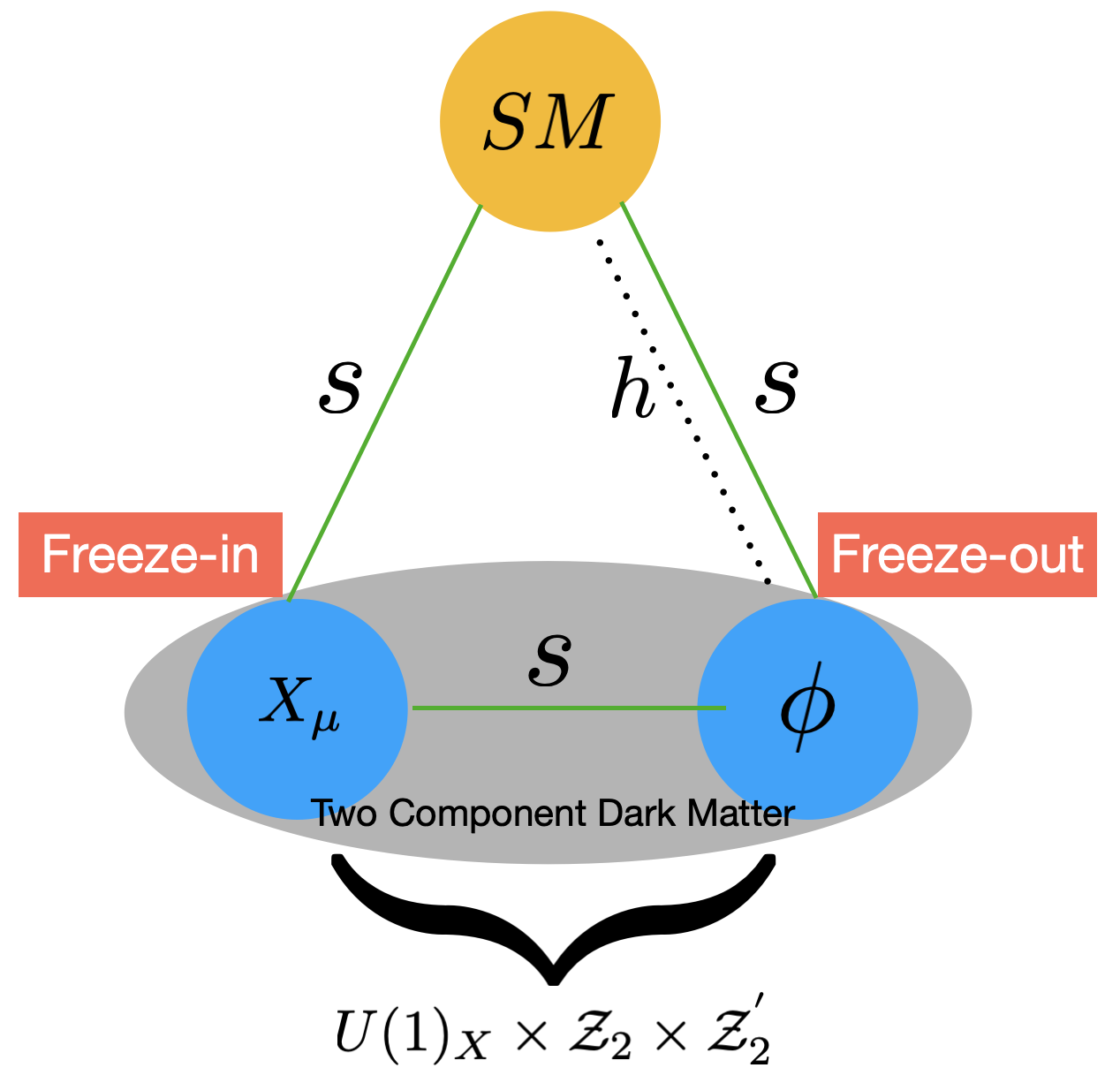
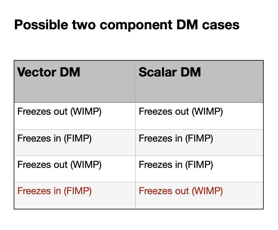
Figure 1: Left: A cartoon depicting the DM components in the model and their interactions to visible sector and amongst them (see text for notation); Right: Possible scenarios in the two component DM set-up, the one in colour is considered in this analysis.

We further note that $X$ being odd under $\mathcal{Z}_{2}$, requires:

$${\mathcal{Z}}_{2}:X\to-X,~{}~{}\implies{\mathcal{Z}}_{2}:S\to S^{*}.$$ (6)

The last relation follows from straightforward calculation. First of all,

$$|{D}^{\mu}S|^{2} =\left[(\partial^{\mu}+ig_{X}X^{\mu})S\right]^{*}\left[(\partial^{\mu}+ig_{X}X^{\mu})S\right],$$ (7)

$$=(\partial^{\mu}-ig_{X}X^{\mu})S^{*}(\partial^{\mu}+ig_{X}X^{\mu})S\,.$$

The transformation of the kinetic piece $|{D}^{\mu}S|^{2}$ under ${\mathcal{Z}}_{2}$ goes as,

$${\mathcal{Z}}_{2}:|{D}^{\mu}S|^{2} =(\partial^{\mu}-ig_{X}X^{\mu})S^{*}(\partial^{\mu}+ig_{X}X^{\mu})S$$ (8)

$$\rightarrow(\partial^{\mu}+ig_{X}X^{\mu})S^{*}(\partial^{\mu}-ig_{X}X^{\mu})S\,.$$

Comparing Eq. 8 with Eq. 7, we get ${\mathcal{Z}}_{2}:S\to S^{*}$.

To summarise, the model inherits two DM components, a VBDM $X$ and a scalar singlet $\phi$ in $U(1)_{X}\times\mathcal{Z}_{2}\times\mathcal{Z}^{{}^{\prime}}_{2}$ extension of SM. Both of them interact with each other and with SM via scalar particle $s$, while $\phi$ also interacts via SM Higgs ($H$) portal. The dark sector particles and their interactions are sketched in a cartoon in the left panel of Fig. 1. Four different phenomenological situations emerge depending on which DM freezes in (FIMP) and which freezes out (WIMP), as shown in the right panel of Fig. 1. We explore the possibility when $X$ is a FIMP and $\phi$ is an WIMP like DM.

3 Possibilities with $X$ freezing-in and $\phi$ freezing-out

Figure 2: The relevant symmetry breaking scales of the model : $U(1)_{X}$ breaking and EWSB (top panel) and different phenomenological situations for $X$ to freeze-in and $\phi$ to freeze-out (bottom panel).

The first noteworthy feature of the model is the presence of two widely different symmetry breaking scales: (i) $SM\times U(1)_{X}\to SM$, and (ii) EWSB: $SU(2)_{L}\times U(1)_{Y}\to U(1)_{EM}$, which are pictorially depicted in Fig. 2. While EWSB scale is known, $U(1)_{X}$ breaking scale crucially depends on whether $X$ freezes in or freezes out. It is explained in a moment. $X$ as FIMP and $\phi$ as WIMP inherit yet another set of phenomenological possibilities that the model offers and are noted in the bottom panel of Fig. 2.

• Freeze-in of $X$ and $U(1)_{X}$ breaking scale: The VBDM $X$ to be a cold DM dictates the scale for $U(1)_{X}$ breaking. The $U(1)_{X}$ gauge coupling ($g_{X}$) which provides DM-SM interaction, is required to be feeble (roughly $g_{X}\sim 10^{-11}$) to keep it out of equilibrium. The DM yield that generates correct relic is proportional to the production cross section (or decay width). For $m_{X}\sim$ TeV, so that it behaves as a cold dark matter (CDM), the $U(1)_{X}$ breaking scale turns out to be $v_{s}\sim 10^{14}$ GeV (following Eq. 5). On the other hand, EWSB occurs at $T_{\rm EW}\sim$ 160 GeV Carena:2004ha ; Baker:2018vos , corresponding to $v_{\rm EW}\sim v$ = 246 GeV. Therefore, the hierarchy $v_{s}\gg v$ implies $T_{U(1)}\gg T_{\rm EW}$ (see Fig. 2), which further aids to the distinction between freeze-in before EWSB (bEWSB) and after EWSB (aEWSB).

  1. Freeze-in bEWSB ($T_{\rm EW}<m_{X}<T_{U(1)}$): When the DM freezes in completely bEWSB, the DM production saturates before $T_{\rm EW}$; then characteristic freeze-in scale is depicted by $T_{\rm{FI}}$ or $x_{\rm{FI}}=\frac{m_{X}}{T_{\rm{FI}}}$ requires

     $$T_{\rm{FI}}>T_{\rm{EW}};~{}\implies x_{\rm{FI}}<x_{\rm{EW}}\,.$$ (9)

     Note also, that the characteristic freeze-in temperature is correlated to the DM mass, $T_{\rm{FI}}\sim m_{X}$. Obviously, $x_{\rm{EW}}=\frac{m_{X}}{T_{\rm EW}}$. In this regime, only the singlet scalar $S$ acquires a vev ($v_{\rm s}$) to give mass to $X$. Other scalars (Higgs and $\phi$) are also massive due to bare mass term, while all the SM fields are massless. In such a situation $X$ has no connection to SM and the production occurs via the interaction with the physical scalar $s$, which is assumed to be in the thermal bath due to sizeable portal coupling with SM Higgs ($H$). The details of the production processes will be discussed in section 4 when we elaborate such a scenario.

  2. Freeze-in aEWSB ($m_{X}\lesssim T_{\rm EW}$): When DM production from thermal bath continues even aEWSB, we have,

     $$T_{\rm{FI}}\sim m_{X}<T_{\rm{EW}};~{}\implies x_{\rm{FI}}>x_{\rm{EW}}\,.$$ (10)

     After EWSB, the Higgs doublet ($H$) acquires a vev ($v$); $H$ and $s$ mix to yield physical scalars $h_{1}$ and $h_{2}$, where $h_{1}$ is assumed to be SM Higgs (dominantly doublet), the one observed at LHC with $m_{h_{1}}\sim$ 125 GeV, while $h_{2}$ is dominantly a singlet, heavier or lighter than the SM Higgs following the existing bounds. Naturally, DM can be additionally produced from the SM particles in thermal bath aEWSB, providing a different allowed parameter space. The detailed discussion is taken up in section 5.

     A cartoon of freeze-in bEWSB (in blue) and aEWSB (in red) is shown in the left panel of Fig. 3 in $Y-x$ plane, where $Y=\frac{n}{\bm{s}}$ refers to DM yield with $\bm{s}$ denoting to entropy density and $x=\frac{m}{T}$, with $m$ denoting DM mass and $T$ denoting temperature of the bath (details in subsection 4.4). From left to right along x-axis, $x$ becomes larger with $T$ dropping. In Fig. 3 (left panel) we consider two DM species denoted by and with $m_{2}>m_{1}$. Following $T_{\rm{FI}}\sim m_{X}$, we have $x_{\rm{FI}}\sim 1$ for both cases. Then following, $x_{\rm{FI}}<x_{\rm{EW}}$ for freeze-in bEWSB, we need $m>T_{\rm{EW}}$, while for freeze-in aEWSB, $x_{\rm{FI}}>x_{\rm{EW}}$ requires $m<T_{\rm{EW}}$. Therefore, we can have $m_{2}>T_{\rm{EW}}>m_{1}$ where freezes in bEWSB and freezes in aEWSB. The red vertical dotted line shows $x_{\rm{FI}}\sim 1$, while pink and blue dotted vertical lines indicate $(x_{1})_{\rm{EW}}$ and $(x_{2})_{\rm{EW}}$ with $(x_{2})_{\rm{EW}}>(x_{1})_{\rm{EW}}$. The relative abundance shown here depends on DM-SM interaction and has no implication unless discussed in context of the model.

• Freeze-out of $\phi$ and EWSB: The real scalar singlet $\phi$ is assumed to be in thermal bath via non-suppressed portal couplings. It freezes out through the dominant $2\to 2$ annihilation to SM and also to other DM candidate (if kinematically allowed). The freeze-out do not crucially dictate any scale in the model unlike freeze-in. Here also, two possibilities emerge:

  1. Freeze-out bEWSB : For $\phi$ to freeze out bEWSB, one requires the characteristic freeze-out temperature ($T_{\rm{FO}}$) to follow,

     $$T_{\rm{FO}}>T_{\rm EW}\implies x_{\rm{FO}}<x_{\rm{EW}}\,;$$ (11)

     where $x_{\rm{FO}}=\frac{m_{\phi}}{T_{\rm{FO}}}$. The processes that are responsible for freeze out of $\phi$ bEWSB are only through the coupling with the physical scalar $s$ and will be elaborated in section 4.

  2. Freeze-out aEWSB : Freeze out of $\phi$ aEWSB implies:

     $$T_{\rm{FO}}<T_{\rm EW}\implies x_{\rm{FO}}>x_{\rm{EW}}\,.$$ (12)

     In this regime, the interaction between $\phi$ and SM arises through $h-s$ mixing and occurs via both the physical scalars $h_{1}$ and $h_{2}$. Therefore, new channels contribute to DM number depletion, we discuss them in details in section 5.

  

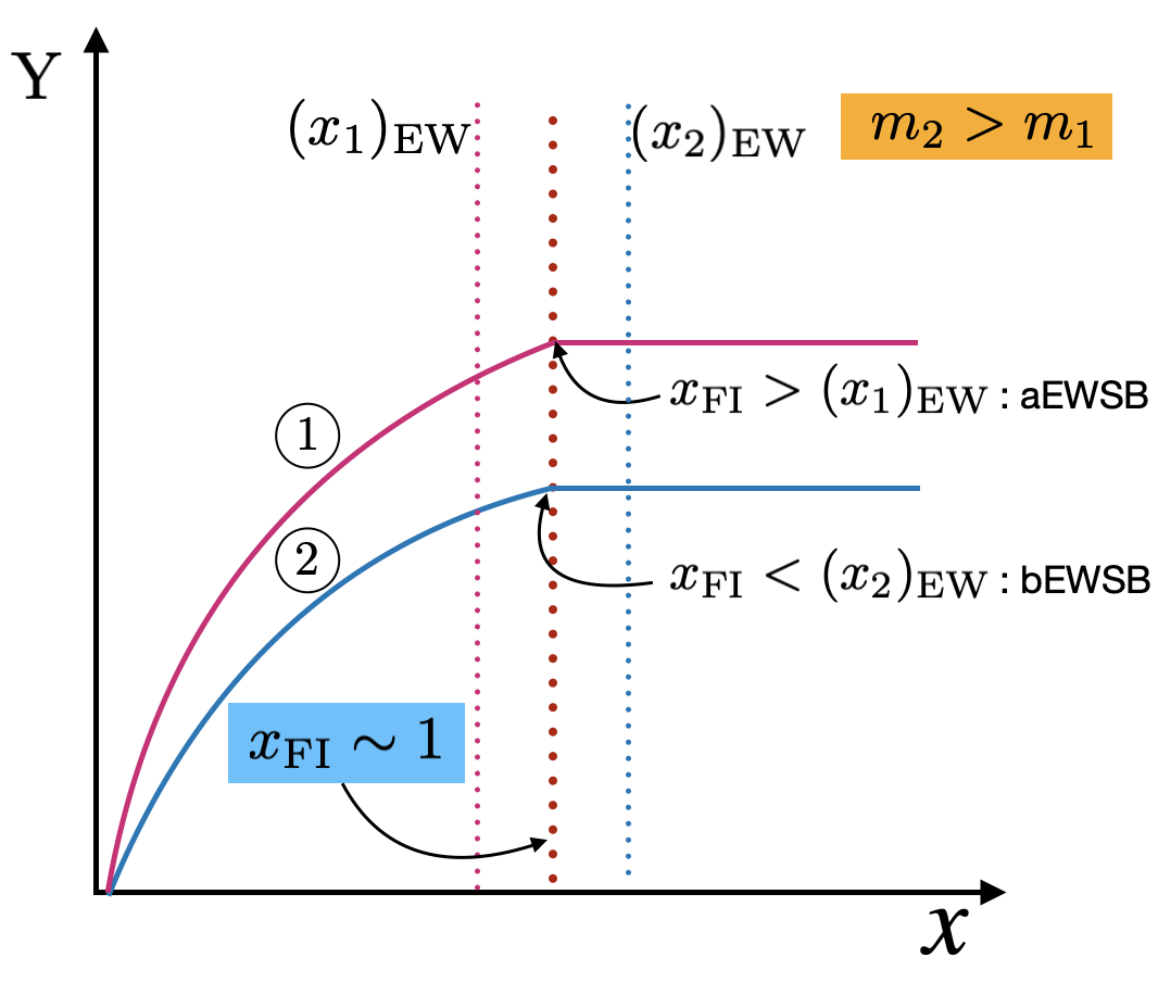
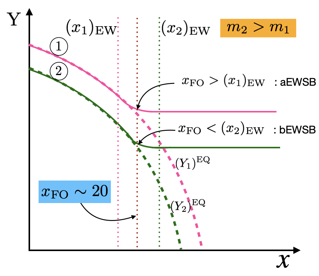
  Figure 3: Left: A cartoon freeze-in in the $Y-x$ plane for two sample DMs with $m_{2}>m_{1}$ which shows freeze-in aEWSB (in red) and bEWSB (in blue). Right: Cartoon freeze-out which shows freeze-out aEWSB (in pink) and bEWSB (in green) from the respective equilibrium distributions (in dashed curves) shown in the right panel.

  Unlike freeze-in, freeze-out of DM does not directly constrain the DM mass. However, for freeze-out to render correct relic density, $x_{\rm{FO}}$ remains in the ballpark $x_{\rm{FO}}\sim 20-25$. Inevitably, freeze-out bEWSB or aEWSB can be realized for different DM masses ($m$), which changes $x_{\rm{EW}}=\frac{m}{T_{\rm EW}}$ to lie above or below $x_{\rm{FO}}$, as depicted in the right panel of Fig. 3. We again consider two DM species denoted by and with $m_{2}>m_{1}$ (shown by green and pink lines); so that $(x_{2})_{\rm{EW}}>(x_{1})_{\rm{EW}}$ (vertical dotted lines) depicts freeze-out bEWSB ($x_{\rm{FO}}<(x_{2})_{\rm{EW}}$) and aEWSB ($x_{\rm{FO}}>(x_{1})_{\rm{EW}}$) respectively from their equilibrium distributions. The distributions and the relative yields in this figure have not been sketched for a particular model or interaction, so the relative strengths have no implications, this is just for the illustration purpose.

Out of different freeze-in epochs of $X$ and freeze-out of $\phi$, as noted in the bottom panel of Fig. 2, we explore two sample cases here with (i) both freeze-in and freeze-out occurring bEWSB and (ii) both occurring aEWSB, which capture the most interesting distinctions of allowed parameter space of the model.

4 Dark Matter phenomenology bEWSB

Here we address in details the freeze-in of $X$ and freeze-out of $\phi$ both occurring bEWSB (option (i) of the bottom panel in Fig. 2.). To be specific, the temperatures around which freeze-in ($T_{\rm{FI}}$) and freeze-out ($T_{\rm{FO}}$) occur, lie between $U(1)_{X}$ breaking and EWSB, i.e.

$$T_{U(1)}>T_{\rm FI}>T_{\rm EW};~{}~{}T_{U(1)}>T_{\rm FO}>T_{\rm EW}\,.$$ (13)

In the following subsections, we discuss the physical particles and interactions in this regime for DM freeze-in and freeze-out via coupled BEQ, relic density and direct search allowed parameter space of the model.

4.1 Physical states and parameters

As the regime is dictated by interactions after spontaneous $U(1)_{X}$ breaking and bEWSB, in unitary gauge we have,

$$S=\frac{1}{\sqrt{2}}(v_{s}+s)\to\langle S\rangle=\frac{1}{\sqrt{2}}v_{s},~{}~{}\langle H\rangle=0,~{}~{}\langle\phi\rangle=0\,.$$ (14)

The scalar potential in this limit reads:

$$V_{\rm scalar}=\mu_{H}^{2}(H^{\dagger}H)+\lambda_{H}(H^{\dagger}H)^{2}+\frac{1}{2}\mu_{\phi}^{2}\phi^{2}+\frac{1}{4!}\lambda_{\phi}\phi^{4}+\frac{1}{2}\mu_{S}^{2}(v_{s}+s)^{2}+\frac{1}{4}\lambda_{S}(v_{s}+s)^{4}$$

$$+\frac{1}{2}\lambda_{\phi H}(H^{\dagger}H)\phi^{2}+\frac{\lambda_{HS}}{2}(H^{\dagger}H)(v_{s}+s)^{2}+\frac{\lambda_{\phi S}}{4}\phi^{2}(v_{s}+s)^{2}\,.$$ (15)

The physical scalars can be identified from extremization of the potential, which provides following relations between the neutral physical scalars and parameters of the model:

$$\begin{split}&\frac{\partial V_{\rm scalar}}{\partial s}=0\to\mu_{S}^{2}=-\lambda_{S}v_{s}^{2}\,,\\ &\frac{\partial^{2}V_{\rm scalar}}{\partial H^{\dagger}\partial H}=m_{H}^{2}\to\mu_{H}^{2}=m_{H}^{2}-\frac{\lambda_{HS}}{2}v_{s}^{2}\,,\\ &\frac{\partial^{2}V_{\rm scalar}}{\partial\phi^{2}}=m_{\phi}^{2}\to\mu_{\phi}^{2}=m_{\phi}^{2}-\frac{\lambda_{\phi S}}{2}v_{s}^{2}\,,\\ &\frac{\partial^{2}V_{\rm scalar}}{\partial s^{2}}=m_{s}^{2}\to\mu_{S}^{2}=m_{s}^{2}-3\lambda_{S}v_{s}^{2}\,;\end{split}$$ (16)

where $m_{H}$ is the mass of the SM like Higgs bEWSB and $m_{\phi}$ is the mass of real scalar DM $(\phi)$ bEWSB. We must note here that $H$ bEWSB represents four massive scalar degrees of freedom (d.o.f) Biswas:2019iqm ; Heeba:2018wtf ; DeRomeri:2020wng ; Chianese:2018dsz being part of the complex isodoublet, while $\phi$ has only one d.o.f being a real scalar singlet. Using Eq. 15 and Eq. 16, it is easy to show that the mass of the $U(1)_{X}$ complex scalar turns out to be $m_{s}^{2}=2\lambda_{S}v_{s}^{2}$. Although $m_{H}$ and $m_{s}$ can be treated as free parameters, they must reproduce correct Higgs mass and mixing, see discussions in the next subsection 4.2 and appendix LABEL:sec:aEWSB-details.

This allows us further to identify the parameters of the model that are relevant for the analysis. All the physical masses and the couplings controlling the relic density of DM are chosen as the external parameters. Quartic self couplings like $\lambda_{H}$ and $\lambda_{\phi}$ are fixed at values within the limit of DM self scattering ($\sim 0.1$) and plays minimal role in DM-SM interaction. All the other parameters are considered as internal parameters which are defined by the relations described in Eqns. 5 and 16. Table 2 summarises the parameters of the model bEWSB. The parameters of the model are subject to further constraints as explained in the next subsection.

External parameters	Internal parameters
$m_{H}$, $m_{s}$, $m_{\phi}$, $m_{X}$, $g_{X}$, $\lambda_{H}$, $\lambda_{\phi}$, $\lambda_{HS}$, $\lambda_{\phi S}$, $\lambda_{\phi H}$	$\mu_{H}$, $\mu_{\phi}$, $\mu_{S}$, $v_{s}$, $\lambda_{S}$

Table 2: External and internal parameters of the model bEWSB.

4.2 Constraints and bounds

In this section, we discuss the possible theoretical and experimental constraints on parameters of the model relevant for our analysis.

• Stability:
  In order to get the potential bounded from below, the quadratic couplings of the potential $V_{\rm scalar}$ must satisfy the following co-positivity conditions as Elias-Miro:2012eoi ; Kannike:2016fmd ; Chakrabortty:2013mha ,

  $$\begin{split}&\lambda_{H}\geq 0,\lambda_{\phi}\geq 0,\lambda_{S}\geq 0,\\ &\lambda_{\phi H}+2\sqrt{\lambda_{H}\lambda_{\phi}}\geq 0,\lambda_{HS}+2\sqrt{\lambda_{H}\lambda_{S}}\geq 0,\lambda_{\phi S}+2\sqrt{\lambda_{\phi}\lambda_{S}}\geq 0\,.\end{split}$$ (17)

  In this analysis, we choose all the couplings positive, which satisfy the above conditions trivially.

• Perturbativity:
  In oder to maintain perturbativity of the theory, the quartic couplings of the scalar potential $V_{\rm scalar}$ and the gauge couplings obey Bhattacharyya:2015nca ; Bhattacharya:2019fgs ,

  $$\begin{split}&\lambda_{H}<4\pi,\hskip 56.9055pt\lambda_{S}<4\pi,\hskip 56.9055pt\lambda_{\phi}<4\pi,\hskip 56.9055ptg_{X}<\sqrt{4\pi},\\ &\lambda_{HS}<4\pi,\hskip 52.92213pt\lambda_{\phi S}<4\pi,\hskip 51.78421pt\lambda_{\phi H}<4\pi\,.\end{split}$$ (18)

• Tree level unitarity:
  Tree level unitarity of the theory, coming from all possible $2\to 2$ scattering amplitude, can be ensured Horejsi:2005da ; Bhattacharyya:2015nca ; Bhattacharya:2019fgs via following constraints

  $$|\lambda_{\phi}|<8\pi,~{}|\lambda_{S}|<4\pi,~{}|\lambda_{H}|<4\pi,~{}|\lambda_{\phi S}|<8\pi,~{}|\lambda_{HS}|<8\pi,~{}|\lambda_{\phi H}|<8\pi\,.$$ (19)

• Constraints on DM mass bEWSB:
  For freeze-in of $X$ to complete bEWSB, it is required that the freeze-in scale ($T_{{\rm FI}}\sim m_{X}$) has to be larger than $T_{\rm{EW}}\sim$ 160 GeV; then, $m_{X}\gtrsim$ 160 GeV. Similarly, freeze-out of $\phi$ bEWSB forces the freeze-out temperature $T_{\rm FO}$ to be larger than $T_{\rm{EW}}$, i.e, $T_{\rm FO}\gtrsim$ 160 GeV. This condition automatically implies that $x_{\rm FO}=m_{\phi}/{T_{\rm FO}}$, which is typically $\sim\$25 for WIMP freeze-out, requires the following condition on WIMP and FIMP masses:

  $${\rm WIMP}:~{}m_{\phi}\gtrsim 4\ {\rm TeV};~{}~{}{\rm FIMP}:~{}m_{X}\gtrsim 160\ {\rm GeV}.$$ (20)

• Relic density: One of the most important constraints on the parameters of the model comes from the observed relic abundance of DM. The latest observations from anisotropies in CMBR in experiments like WMAP WMAP:2012nax , and PLANCK Planck:2018vyg indicate

  $$\Omega_{\rm DM}h^{2}=\Omega_{X}h^{2}+\Omega_{\phi}h^{2}=0.1200\pm 0.0012\,,$$ (21)

  where $\Omega=\frac{\rho}{\rho_{c}}$ refers to cosmological density, with $\rho_{c}$ indicating critical density, $h$ is the present Hubble parameter scaled in units of 100 km/s/Mpc. In the two component WIMP-FIMP set up that we explore here, the individual relic densities of $X$ and $\phi$ shall add to the total observed relic, where each of the individual components will be under-abundant, ie, $\Omega_{X,\phi}h^{2}\lesssim 0.12$. We elaborate on the relic density of the WIMP and FIMP components of the model in the next section.

• Direct detection (DD) constraints: WIMP ($\phi$) has a direct search prospect, while the FIMP ($X$) does not . In this regime, although freeze out of $\phi$ occurs bEWSB, after EWSB $\phi$ couples to SM, yielding a possibility of direct search of $\phi$. Non observation of DM from ongoing experiments like XENON1T XENON:2018voc sets an stringent upper limit on WIMP-nucleon spin-independent elastic scattering cross-section at 90% C.L,

  $$\begin{split}\sigma_{\rm{SI}}\sim\begin{cases}4.1\times 10^{-47}~{}\rm{cm}^{2}~{}~{}\rm{~{}~{}~{}~{}at~{}30~{}GeV/c^{2}~{}~{}(XENON1T)}\\ 1.4\times 10^{-48}~{}\rm{cm}^{2}~{}~{}\rm{~{}~{}~{}~{}at~{}50~{}GeV/c^{2}~{}~{}(XENONnT)}\end{cases}\end{split}$$ (22)

  Here, we also mention the projected XENONnT XENON:2020kmp sensitivity. The relevant couplings $g_{X}$ and $\lambda_{\phi S}$, are constrained to be $\sim 10^{-12}$ both from the freeze-in requirements and direct search bounds. In addition, $\lambda_{\phi H}\sim 10^{-3}$ keeps the DD cross section safely below the experimental direct search bounds. We provide a detailed account for direct search of the model in the Appendix D.

• Higgs mass and mixing: It is important to note that independent of DM freeze-out or freeze-in to occur bEWSB or aEWSB, there is a mixing of Higgs ($h$) with $s$ after EWSB to render two physical states: $h_{1}$, assumed to be SM like Higgs with $m_{h_{1}}=125.1$ GeV and a heavy or light $h_{2}$, dominantly a singlet. $h-s$ mixing angle ($\theta$) is restricted by LHC data Chalons:2016lyk within:

  $$|\sin\theta|\lesssim 0.3\,.$$ (23)

  The requirement of correct Higgs mass as well as mixing puts limit on parameters $m_{H},m_{s},\lambda_{HS}$ etc. For details of the mass eigenstates, mixing and relations with model parameters, refer to the discussions in appendix LABEL:sec:aEWSB-details. We note here one important exception, if $m_{s}\gtrsim 2m_{X}$ then dominant FIMP production occurs from $s$ decay, and additionally if the FIMP production from late decay of $s$ saturates bEWSB, then there is no $s$ which remains in the bath to mix with $h$ and consequently no $h_{2}$ state to appear aEWSB. Then Higgs mass bEWSB and aEWSB are related by $m_{H}^{2}=\frac{m_{h_{1}}^{2}}{2}$. Note further, collider bound on scalar singlet WIMP DM mass $m_{\phi}$ is mild Barger:2007im ; Fuchs:2020cmm , while no significant bound on FIMP mass can be obtained.

• Invisible Decay of Higgs : SM Higgs ($h_{1}$) can decay into pairs of DM ($X$ and $\phi$) as well as to pairs of $h_{2}$ in our model if kinematically allowed. Since these decays contribute to invisible decay of Higgs, corresponding $h_{1}\phi\phi,~{}h_{1}XX,~{}h_{1}h_{2}h_{2}$ couplings get severely constrained by the experimental data. They can be traced from expressions of Higgs decay width to $\phi,X,h_{2}$ as provided in Appendix C. As per the latest experimental data given by ATLAS (for 139 $fb^{-1}$ luminosity at $\sqrt{s}=13$ TeV), the strictest upper limit on $\mathcal{B}_{h_{1}\to\text{inv}}$ can be set to $\sim$  0.13 at 95% CL Milosevic:2020xup ; ATLAS:2020kdi ; Okawa:2020jea . A comparison of the invisible Higgs decay bound from latest ATLAS and CMS data is given by:

  $$\begin{split}&\mathcal{B}_{h_{1}\to\rm{inv}}<\begin{cases}0.13~{}~{}~{}\rm(ATLAS)\\ 0.19\rm~{}~{}~{}(CMS)\end{cases}\\ &\Gamma_{h_{1}\to\rm{inv}}<\begin{cases}0.61\rm{~{}MeV}~{}~{}~{}\rm(ATLAS)\\ 0.95\rm{~{}MeV}~{}~{}~{}(CMS)\end{cases}\end{split}$$ (24)

  For simplicity, we do not scan the region of parameter space where Higgs invisible decay to DM is possible, with $m_{X}>m_{h_{1}}/2$, and $m_{\phi}>m_{h_{1}}/2$. However, $h_{2}\to XX$ is considered for the analysis, where there is no bound.

4.3 Processes contributing to DM Relic

The processes that contribute to freeze-in of vector boson $X$ bEWSB are shown in Fig. 4. The initial abundance of $X$ in the early universe is assumed negligible, while it builds up via production from the particles in thermal bath, namely $s,\phi$ and $H$. Decay of $s$ contributes the most, subject to the kinematic constraint $m_{s}\geq 2m_{X}$. Scattering processes $ss\to XX$ also contribute but it is suppressed compared to the decay. In addition, $HH^{\dagger}\to XX$ and $\phi\phi\to XX$ also contribute, mediated by s-channel $s$. The process $\phi\phi\to XX$ is WIMP-FIMP conversion and it occurs as $\phi$ is assumed present in the thermal bath. We will discuss the effect of such conversion contributions in details. It is worth noting that unsuppressed $ss\to H^{\dagger}H,~{}\phi\phi\to H^{\dagger}H,~{}\phi\phi\to ss$ keep $\phi,~{}s,~{}$and $H$, all in equilibrium in early universe. The processes which contribute to freeze out of $\phi$ bEWSB are shown in Fig. 5. They are all known, and include $\phi\phi\to HH^{\dagger}$ via the quartic coupling as well as that mediated by $s$; additionally $\phi\phi\to ss$ occurs via quartic portal coupling, and s-channel mediation by $s$ and t-channel mediation by $\phi$. Finally, WIMP-FIMP conversion $\phi\phi\to XX$ via s-channel mediation of $s$ is also possible as shown in the bottom panel of Fig. 5, otherwise absent in single component case. Let us recall again that all the processes initiated by $H$ and those produce $H$ assume four massive scalar d.o.f.

Figure 4: Feynman diagrams showing non-thermal production channels of $X$ bEWSB.

Figure 5: Feynman diagrams contributing to $\phi$ freeze-out via $2\to 2$ depletion processes bEWSB.

4.4 Coupled Boltzmann Equations and conversion

The DM number density for the WIMP-FIMP scenario can be evaluated by the coupled Boltzmann equations (cBEQs):

$$\frac{dY_{X}}{dx}= \,-\,\frac{2\,{\rm M_{Pl}}}{1.66}\frac{x}{m_{X}^{2}}\frac{\sqrt{g_{*}(x)}}{g_{s}^{*}(x)}\langle\Gamma_{s\to XX}\rangle\left(Y_{X}-Y_{s}^{eq}\right)\$$

$$- \frac{4\pi^{2}{\rm M_{Pl}}\sqrt{g_{*}(x)}}{45\times 1.66}\frac{m_{X}}{x^{2}}\left[\sum_{i=s,H}\langle\sigma\mathpzc{v}\rangle_{ii\to XX}\left(Y_{X}^{2}-(Y_{i}^{eq})^{2}\right)-\langle\sigma\mathpzc{v}\rangle_{\phi\phi\to XX}\left(Y_{\phi}^{2}-\frac{(Y_{\phi}^{eq})^{2}}{(Y_{X}^{eq})^{2}}Y_{X}^{2}\right)\right],$$ (25)

$$\frac{dY_{\phi}}{dx}= -\frac{2\pi^{2}\,{\rm M_{Pl}}\sqrt{g_{*}(x)}}{45\times 1.66}\frac{m_{\phi}}{x^{2}}\left[\sum_{i=s,H}\langle\sigma\mathpzc{v}\rangle_{\phi\phi\to ii}\left(Y_{\phi}^{2}-(Y_{\phi}^{eq})^{2}\right)+\langle\sigma\mathpzc{v}\rangle_{\phi\phi\to XX}\left(Y_{\phi}^{2}-\frac{(Y_{\phi}^{eq})^{2}}{(Y_{X}^{eq})^{2}}Y_{X}^{2}\right)\right]\,.$$ (26)

In the above, $x=m/T,~{}Y_{X,\phi}=\frac{n_{X,\phi}}{\bm{s}}$, where $n_{X,\phi}$ refers to the number of $X\text{ and }\phi$ respectively, and $\bm{s}$ represents entropy density given by $\bm{s}=\frac{2\pi^{2}}{45}g_{*}^{s}(T)T^{3}$. The equilibrium number density with respect to comoving volume for non-relativistic species ($X,\phi$) is given by Boltzmann distribution (assuming chemical potential to be zero)

$$Y^{eq}=\frac{n^{eq}}{\bm{s}}=0.145\frac{g}{g^{s}_{*}}x^{3/2}e^{-x}.$$

Further note $\sqrt{g_{*}(T)}\simeq\frac{g^{s}_{*}(T)}{\sqrt{g^{\rho}_{*}(T)}}$, where $g^{s}_{*}$ and $g^{\rho}_{*}$ denote d.o.f corresponding to entropy and energy density of the Universe. Further, $\rm{M_{Pl}}=1.22\times 10^{19}$ GeV denotes reduced Planck mass. Thermal average of decay width $\langle\Gamma_{A\to BB}\rangle$ and annihilation cross-section times the velocity $\langle\sigma\mathpzc{v}\rangle_{AA\to BB}$ are given by,

$$\langle\Gamma_{A\to BB}\rangle = \Gamma_{A\to BB}\frac{K_{1}\left(m_{B}/T\right)}{K_{2}\left(m_{B}/T\right)},$$

$$\langle\sigma\mathpzc{v}\rangle_{AA\to BB} = \frac{1}{8m_{A}^{4}TK_{2}^{2}(m_{A}/T)}\int_{4m_{B}^{2}}^{\infty}d\mathtt{s}\ \sigma_{AA\to BB}(\mathtt{s})(\mathtt{s}-4m_{A}^{2})\sqrt{\mathtt{s}}\,K_{1}\left(\sqrt{\mathtt{s}}/T\right).$$ (27)

$K_{1,2}$ are modified Bessel functions of first and second kind respectively and $\mathpzc{v}$ refers to M$\ddot{o}$llar velocity defined by $\mathpzc{v}=\frac{\sqrt{(p_{1}.p_{2})^{2}-m_{1}^{2}m_{2}^{2}}}{E_{1}E_{2}}$. In $\langle\Gamma_{A\to BB}\rangle$, the particle ($A$) is decaying at rest and the thermal average do not involve an integration over the centre-of-mass energy $\sqrt{\mathtt{s}}$, while for annihilation cross-section $\langle\sigma\mathpzc{v}\rangle_{AA\to BB}$, a lower limit $\mathtt{s}=4m_{B}^{2}$ is required for the reaction to occur and it diminishes at high $\sqrt{\mathtt{s}}$, owing to the presence of $K_{1}\left(\sqrt{\mathtt{s}}/T\right)$ for a particular $T$.

One important point to note before we proceed further. The WIMP-FIMP conversion $\phi\phi\to XX$, which makes the BEQs (Eq. 25 and 26) coupled, requires to be of the order of freeze-in production cross-section, as otherwise it will thermalize the FIMP, suppressing the non-thermal production (this exercise will be discussed in details elsewhere). This in turn, makes conversion process negligible compared to other annihilation cross-sections of $\phi$ (first term in Eq. 26). However, this conversion can still be significant for non-thermal production of $X$. This feature is generic to any two-component WIMP-FIMP model, where the freeze-out of WIMP can be marked unaffected by the conversion to FIMP, while the FIMP production can be substantial due to WIMP. This feature importantly reduces the cBEQs as in Eq. 25 and Eq. 26 to two individual uncoupled BEQs, where the conversion can be dropped from Eq. 26 to yield:

$$\frac{dY_{X}}{dx}= \frac{2\,{\rm M_{Pl}}}{1.66\sqrt{g^{\rho}_{*}(x)}}\frac{x}{m_{X}^{2}}\langle\Gamma_{s\to XX}\rangle Y_{s}^{eq}$$

$$+\frac{4\pi^{2}\,{\rm M_{Pl}}}{45\times 1.66}\frac{g^{s}_{*}(x)}{\sqrt{g^{\rho}_{*}(x)}}\frac{m_{X}}{x^{2}}\left(\sum_{i=s,H}\langle\sigma\mathpzc{v}\rangle_{ii\to XX}(Y_{i}^{eq})^{2}+\langle\sigma\mathpzc{v}\rangle_{\phi\phi\to XX}Y_{\phi}^{2}\right),$$ (28)

$$\frac{dY_{\phi}}{dx}= -\frac{2\pi^{2}\,{\rm M_{Pl}}}{45\times 1.66}\frac{g^{s}_{*}(x)}{\sqrt{g^{\rho}_{*}(x)}}\frac{m_{\phi}}{x^{2}}\sum_{i=s,H}\langle\sigma\mathpzc{v}\rangle_{\phi\phi\to ii}\left(Y_{\phi}^{2}-(Y_{\phi}^{eq})^{2}\right).$$ (29)

Eq. 28 and 29 allow us to treat the freeze-in of $X$ and freeze-out of $\phi$ separately as we do next. It also allows to treat $x=m_{X}/T$ in Eq. 28 and $x=m_{\phi}/T$ in Eq. 29 as two separate variables . We further note that in view of small $Y_{X}$ and feeble interaction, we have dropped the terms $\propto Y_{X}$ and $Y_{X}^{2}$ ($X\,X\to s$ and $X\,X\to i\,i$) in Eq. 25 to obtain Eq. 28.

4.5 Freeze-in of X

Now let us discuss the freeze-in of $X$, bEWSB in details. The main point is that the initial abundance of $X$ in the early universe is negligible, builds up from the decay or scattering of the particles in thermal bath and saturates when the photon temperature falls below DM mass. One essentially then needs to solve BEQ. 28 from $x\simeq 0$ to $x=m_{X}/T_{\rm{EW}}$, using non-thermal production of $X$, indicated in Fig. 4, and include: 1. $s$decays to $X$ pair while in thermal equilibrium and after $s$ freezes out, 2. $s$and $H$ scattering to $X$ pairs, 3. $\phi$pair annihilation to $X$ pairs.

However, there is a slight twist to the story. The decay contribution of $s$ to $X$ pairs as written in Eq. 28 is only applicable when the decaying particle is in equilibrium with the thermal bath. The decay process however continues even after $s$ freezes out from thermal bath, i.e. beyond $x\geq x_{D}$, where $x_{D}$ denotes freeze-out point of $s$. The decay contribution after freeze-out of $s$ from thermal bath is often termed as ‘late decay’ (LD) of $s$. The dynamics of such effect can be captured by yet another coupled BEQ written together with the evolution of yield $Y_{s}$ (see Appendix LABEL:sec:bEWSB-details), where the freeze out of $s$ is governed by its annihilation channels to SM, as shown in Feynman graph in Fig. 6. The coupled BEQ for this case can be simplified to a single BEQ with an additional term to in-equilibrium decay (for derivation, see Barman:2019lvm ; Buch:2016jjp ):

$$\frac{dY_{X}}{dx}= \frac{45}{3.32\pi^{4}}\frac{g_{s}\,M_{{\rm Pl}}\,m_{s}^{2}\,\Gamma_{s\to XX}}{m_{X}^{4}}\left(\frac{x^{3}K_{1}\left[\frac{m_{s}}{m_{X}}x\right]}{g^{s}_{*}(x)\sqrt{g_{*}^{\rho}(x)}}\Theta\left(x_{D}-x\right)\right.$$

$$\left.+\ e^{-\frac{0.602\,M_{{\rm Pl}}\,\Gamma_{s\to XX}}{m_{X}^{2}\sqrt{g^{\rho}_{*}(x)}}(x^{2}-x_{D}^{2})}\frac{x^{2}x_{D}}{\eta(x,x_{D})}K_{1}\left[\alpha(x,x_{D})\frac{m_{s}}{m_{X}}\frac{x^{2}}{x_{D}}\right]e^{\frac{m_{s}}{m_{X}}\left(\alpha(x,x_{D})\frac{x^{2}}{x_{D}}-x_{D}\right)}\Theta(x-x_{D})\right)$$

$$+\frac{4\pi^{2}\,\rm{M_{Pl}}}{45\times 1.66}\frac{g^{s}_{*}(x)}{\sqrt{g^{\rho}_{*}(x)}}\frac{m_{X}}{x^{2}}\left(\sum_{i=s,H}\langle\sigma\mathpzc{v}\rangle_{ii\to XX}(Y_{i}^{eq})^{2}+\langle\sigma\mathpzc{v}\rangle_{\phi\phi\to XX}Y_{\phi}^{2}\right).$$ (30)

In the above, the term proportional to $\Theta(x_{D}-x)$ in the first parenthesis indicates FIMP production from ‘in-equilibrium’ decay of $s$ and the second term in the first parenthesis captures the late decay contribution with $\Theta(x-x_{D})$ denoting the Heaviside theta function. Also note that $g_{s}$ (internal d.o.f for $s$) is 1. The freeze out point of $s$ is denoted by $x_{D}$ which can be found out by following expression:

$$x_{D}={\rm ln}[\Lambda]-\frac{1}{2}{\rm ln[ln}[\Lambda]],\ \Lambda=0.038~{}\frac{g_{s}m_{s}\rm{M_{Pl}}}{\sqrt{g^{\rho}_{*}}}\sum_{SM=H,\phi,X}\sigma^{0}_{ss\rightarrow\rm{SM~{}SM}},$$ (31)

where $\sigma^{0}_{ss\rightarrow\rm{SM~{}SM}}$ denotes annihilation cross-section of $s$ to SM particles at threshold ($\mathtt{s}=4\,m^{2}_{{\rm s}}$) and corresponding expressions are provided in the appendix LABEL:sec:bEWSB-details. Also note in Eq. 30, the factor $\eta(x,x_{D})$ and $\alpha(x,x_{D})$ are given by:

$$\eta(x,x_{D})=\alpha(x,x_{D})g_{*}^{s}(x)\sqrt{g_{*}^{\rho}(x)},~{}~{}\alpha(x,x_{D})=\left[\frac{g_{*}^{s}(x_{D})}{g_{*}^{s}(x)}\right]^{1/3}\ \left[\frac{g_{*}^{\rho}(x_{D})}{g_{*}^{\rho}(x)}\right]^{1/4}.$$ (32)

Figure 6: Feynman diagrams showing all possible annihilation channels of $s$, which causes $s$ to freeze out from thermal bath bEWSB.

Late decay contribution provides significant contribution to DM yield. However, when we consider freeze-in to occur bEWSB, late decay contribution should also accumulate fully bEWSB. This evidently requires freeze-out of $s$ to occur bEWSB with $T_{D}>T_{\rm{EW}}$, with $x_{D}=\frac{m_{s}}{T_{D}}$ (see Eq. 31 for details) varying typically in the range of $\sim 20-25$. We can achieve this limit by having heavy $m_{s}$ for which $x_{D}\leq m_{s}/T_{\rm{EW}}$, resulting a limit on $m_{s}$ as:

$$T_{\rm EW}\lesssim\frac{m_{s}}{25}\implies m_{s}\gtrsim 4~{}\rm{TeV}\,,$$ (33)

which is not surprisingly the same limit on WIMP mass to freeze-out bEWSB as in Eq. 20.

The yield of $X$ in the pre-EWSB regime is given by,

$$Y_{X}^{{\rm bEWSB}} =\frac{45}{3.32\pi^{4}}\frac{{\rm M_{Pl}}\,m_{s}^{2}\,\Gamma_{s\to XX}}{m_{X}^{4}}\int_{0}^{m_{X}/T_{\rm{EW}}}\biggl{[}\frac{x^{3}K_{1}\left[\frac{m_{s}}{m_{X}}x\right]}{\sqrt{g_{*}^{\rho}(x)}g^{s}_{*}(x)}\Theta\left(x_{D}-x\right)$$

$$+\ e^{-\frac{0.602\,{\rm M_{Pl}}\,\Gamma_{s\to XX}}{m_{X}^{2}\sqrt{g^{\rho}_{*}(x)}}(x^{2}-x_{D}^{2})}\frac{x^{2}x_{D}}{\eta(x,x_{D})}K_{1}\left[\alpha(x,x_{D})\frac{m_{s}}{m_{X}}\frac{x^{2}}{x_{D}}\right]e^{\frac{m_{s}}{m_{X}}\left(\alpha(x,x_{D})\frac{x^{2}}{x_{D}}-x_{D}\right)}\Theta(x-x_{D})\biggr{]}dx$$

$$+\frac{45\,{\rm M_{Pl}}}{4\pi^{6}\times 1.66}\int_{0}^{m_{X}/T_{\rm{EW}}}\sum_{i=s,H}\langle\sigma\mathpzc{v}\rangle_{ii\to XX}~{}\frac{m_{i}^{4}}{m_{X}^{3}}\frac{x^{2}K_{2}^{2}\left[\frac{m_{i}}{m_{X}}x\right]}{g_{*}^{s}(x)\sqrt{g_{*}^{\rho}(x)}}dx$$

$$+\frac{4\pi^{2}\rm{M_{Pl}}m_{X}}{45\times 1.66}\int_{0}^{m_{X}/T_{\rm{EW}}}\langle\sigma\mathpzc{v}\rangle_{\phi\phi\to XX}~{}\frac{g_{*}^{s}(x)}{\sqrt{g_{\rho}^{*}(x)}}\frac{Y_{\phi}^{2}}{x^{2}}dx\,.$$ (34)

We note that although the limit of $x$ integration above is taken upto EWSB scale ($x:0\to m_{X}/T_{\rm{EW}}$), the result does not alter if we extend the limit to smaller temperature or larger $x\to\infty$, as the parameters are chosen in a way that freeze-in occurs bEWSB. Freeze-in bEWSB is ensured by checking $Y_{x>x_{EW}}=Y_{x_{EW}}$. Finally, the relic density for $X$ can be written in terms of $Y_{X}$ and we want to probe under abundant region, as $X$ constitutes a part of two component framework, then,

$$\Omega_{X}\rm h^{2}\simeq 2.744\times 10^{8}\ m_{X}Y_{X}^{\rm{bEWSB}};~{}~{}\Omega_{X}\rm h^{2}\leq 0.1212\,.$$ (35)

where the FIMP dark matter relic density is written in terms of the reduced Hubble parameter, $h$ in units of 100 km/s/Mpc.

4.5.1 Phenomenology

As argued before, FIMP production from decay is always dominant over the scattering processes in our model due to the presence of either feeble couplings at both vertices, a heavy mediator or heavy initial state particles for the latter. Therefore, in this study we can divide the FIMP parameter space into two purely separate mass regimes, where decay and scattering contributions to FIMP production are mutually exclusive. However, in cases where scattering can create a heavy mediator on-shell with unsuppressed production and decays subsequently to DM, there may arise a potential double counting when both decay and scattering processes are considered together Belanger:2018ccd , which needs to be accounted. For us there is no such issue with the following segregation of kinematic regimes which yield different phenomenology:

• Case-I ($m_{s}\geq 2m_{X}$): $X$ is produced mainly from $s$ decay, annihilation processes are smaller and neglected.

• Case-II ($m_{s}<2m_{X}$): Decay channel ($s\to XX$) is forbidden, scattering processes contribute to $X$ production.

Case-I $\left(m_{s}\geq 2m_{X}\right):$

In this kinematical region, given that even late decay of $s$ occurs bEWSB, it leaves no trace of $s$ aEWSB. So, there is no $s-H$ mixing and dark sector remains detached from the SM. As mentioned previously, for this case, we need to choose $m_{H}^{2}=m_{h_{1}}^{2}/2$ to get the correct Higgs mass aEWSB. Together we also demand that $\phi$ freezes-out bEWSB, then DM components do not have any direct coupling to SM, except the quartic interaction $\phi\phi\to HH$ proportional to $\lambda_{\phi H}$. But as discussed, constraints from Direct search on $\lambda_{\phi H}$ makes this coupling weak, this particular kinematical region with freeze-in and freeze-out both occurring bEWSB, is difficult to probe by any experiment in the near future and is thus constrained very feebly by direct detection or collider search constraints.

(a)

(b)

(c)

(d)

(e)

Figure 7: Freeze-in for $X$ bEWSB in relic density ($\Omega_{X}h^{2}$) versus $x=\frac{m_{X}}{T}$ plane obtained by solving BEQ (Eq. 30) for the kinematic region $2m_{X}\leq m_{s}$. Fig. 7a, 7b, 7c, 7d shows variation with respect to parameters $m_{s},m_{X},g_{X},\lambda_{HS}$, having three different values where one provides correct relic, one under abundance and one over abundance. Parameters chosen for the plot are mentioned in figure inset and heading. Horizontal black dashed line shows correct relic density. The vertical dot-dashed lines indicate EWSB. Fig. 7e shows late decay contribution of $s$ to freeze-in of $X$ bEWSB, obtained by solving cBEQ (Eq. LABEL:cbeq_sX) using Mathematica.

The plots in Fig. 7 show change in $\Omega_{X}h^{2}$ in terms of $x=m_{X}/T$ where freeze-in necessarily occurs bEWSB. All the plots are generated by solving BEQ (Eq. 30) using Mathematica. In Fig. 7a, three different coloured lines in red, blue, green correspond to three different values of $m_{s}$ (mentioned in figure inset with other parameters kept fixed are mentioned in the figure heading), so that $X$ freezes-in bEWSB. The vertical blue dotted line shows EWSB $(x_{\rm{EW}}=m_{X}/T_{\rm{EW}}$). As $X$ is produced from $s$ decay (and late decay of $s$), where the decay width of $s$ is proportional to $m_{s}$, it is clear that with larger $m_{s}$, the $X$ abundance increases. We also see that the entire freeze-in of $X$, takes place in two steps. Firstly, when $s$ is in equilibrium i.e., for $T>T_{D}$ ($T_{D}$ denotes freeze-out point of $s$), then $X$ yield increases from zero and reaches the first plateau when $T<m_{X}$. Afterwards, when $T$ drops to $T\lesssim T_{D}$, then $s$ freezes out and the late decay of $s$ into $X$ is activated, $X$ yield rises again, eventually producing the second plateau. The horizontal black dotted line represents the central value of the present DM relic abundance. We see that the blue line with $m_{s}=14$ TeV matches to correct relic, given other parameters fixed as mentioned in the figure heading. Also note here that we choose $x=0.001$ to start the freeze-in production, although ideally the maximum temperature of the bath ($T_{\rm{RH}}$) should be very high $T_{\rm{RH}}\sim T_{U(1)}$. This is simply because, in both decay and scattering dominated freeze-in of $X$ in this model, the yield is independent of $T_{\rm{RH}}$, a typical feature of IR freeze-in.

In Fig. 7b, 7c and 7d, we show how the freeze-in of X depends on the parameters $m_{X},~{}g_{X}$ and $\lambda_{HS}$ when $s$ decay is the main source of $X$ production. In each plot three cases are shown, one for correct relic, one for under abundance and one for over abundance. The values of the parameters kept fixed to achieve them can be read from figure insets and headings. As the resultant yield is proportional to the decay width of $s$, the dependence of these parameters on the decay width solely determine the relic density accumulated. For example, $m_{X}$ is inversely proportional to $s$ decay width. Therefore, with larger $m_{X}$, the relic density decreases in Fig. 7b. On the other hand, $s$ decay width is proportional to $g_{X}$, therefore $X$ relic density increases with larger $g_{X}$ as is clear from Fig. 7c. In Fig. 7d, we have shown the dependence on $\lambda_{HS}$. The decoupling of $s$ from thermal bath depends on $\lambda_{HS}$. With larger $\lambda_{HS}$, $s$ annihilation cross-section increases, delaying the decoupling of $s$ which in turn reduces the late decay contribution to $X$ yield, as evident from Fig. 7d.

The very fact that the late decay contribution of $s$ is essentially that of freeze-out abundance of $s$ converting into $X$ yield, is clear when we solve the coupled BEQ for $s$ freeze-out and $X$ freeze-in together as elaborated in Appendix LABEL:sec:bEWSB-details (see Eq. LABEL:cbeq_sX) and demonstrated in Fig. 7e. Here, the green line represents the variation of $X$ yield ($Y_{X}$) with $m_{s}/T$ and the red line represents $Y_{s}$. $Y_{s}$ shows the freeze-out of $s$ from the equilibrium distribution and then late decay to $X$ (descending part of $s$ yield after freeze out). The freeze-out yield of $Y_{s}$ matches to $Y_{X}$ yield completely. The vertical green dashed line confirms that the entire phenomenon occurs bEWSB for the chosen parameters of the model.

(a)

(b)

(c)

Figure 8: Numerical scan of the under-abundant region of $X$ relic (Eq. 35) for freeze in bEWSB, when $\left(2m_{X}\leq m_{s}\right)$. Figs. 8a shows scan in $m_{X}-g_{X}$ plane, 8b in $g_{X}-\lambda_{HS}=\lambda_{\phi S}$ plane and 8c in $m_{s}-m_{X}$ plane. Different colour shades indicate different ranges of relic density for fixed values of other parameters within our said bound as mentioned in figure inset and caption. The rainbow colour bar represents the contribution of the late decay of $s$ in $X$ freeze-in by the ratio $\left(\Omega_{\rm{LD}}/\Omega_{X}\right)$. This kinematic region is free from collider and direct search constraints, see text for details.

We find out next the relic under abundant parameter space of the model (Eq. 35) via numerical scan for the kinematic region $2m_{X}\leq m_{s}$ in Fig. 8. Fig. 8a shows the parameter space in $g_{X}$ vs. $m_{X}$ plane. The color shades in light yellow, light red and light blue indicate different ranges of relic density (see Fig. inset). The scattered points with shades as in the color bar signify the percentage of ‘late decay’ contribution to the relic density of $X$ ($\Omega_{\rm{LD}}h^{2}$) with respect to the total $X$ relic density ($\Omega_{X}h^{2}$). The variation of relic density with $g_{X}$ and $m_{X}$ is consistent with the behaviour already noted in Fig. 7b and 7c, as we show that relic density increases with increasing $g_{X}$ and decreasing $m_{X}$. This is also true for the scattered points, as the functional dependence of the parameters are the same for both in-equilibrium decay and the late decay of $s$. In other two correlation plots, i.e., Fig. 8b (scan in $g_{X}-\lambda_{HS}$ plane) and Fig. 8c (scan in $m_{s}-m_{X}$ plane), we find that the change in relic density is consistent with Fig. 7a and Fig. 7d. In all these three correlation plots, we mark the overabundant region with light grey shaded region and the deep grey area signifies the parameter region where freeze-in bEWSB condition is not maintained. We further note that as only decay of $s$ dominates the production of $X$, Higgs mixing does not appear aEWSB and so collider bound is mostly absent. DD cross-section (the discussion is postponed to appendix D as it is a standard exercise) is only affected by $\lambda_{\phi H}$ parameter, which is not very sensitive to the decay dominated production, especially when $m_{\phi}$ is in TeV range. This makes the parameter space free from the experimental constraints. We must also note that for all plots bEWSB in the kinematic region $2m_{X}\leq m_{s}$, the choice of $m_{H}=m_{h_{1}}/\sqrt{2}=88.46$ GeV is consistent with a SM Higgs with $m_{h_{1}}=125.1$ GeV.

Case-II: $\left(m_{s}\lesssim 2m_{X}\right):$

Now, we consider a kinematic region where $s$ decay is kinematically forbidden to produce $X$, with $m_{s}<2m_{X}$. Absence of decay (and late decay) indicates that scattering, as shown in Fig. 4, plays a crucial role in the production of $X$. If $X$ is produced through scattering or WIMP-FIMP conversion bEWSB, then $s$ remains in the thermal bath to mix with $h$ after EWSB, eventually connecting DM to SM. In this case, DD remains a viable option for detection of WIMP (see appendix D). Also the mixing angle ($\sin\theta$) of $s$ and the CP-even neutral component of Higgs doublet is restricted by the upper bound on mixing obtained from collider search as $\sin\theta\leq\mathcal{O}(0.3)$ Chalons:2016lyk . On top of that, following the correlation between $\lambda_{HS}$ and $\sin\theta$ as in Eq. 60, $\lambda_{HS}$ will get further constrained by the mixing bounds, and constrain the parameter space bEWSB. On the contrary, when FIMP production completes bEWSB via $s$ decay (and late decay), $\lambda_{HS}$ remains mostly unconstrained due to absence of $s$ aEWSB.

(a)

(b)

Figure 9: Freeze-in production for $X$ bEWSB in relic density ($\Omega_{X}h^{2}$) versus $x=\frac{m_{X}}{T}$ plane for the kinematic region $m_{s}<2m_{X}$, when scattering processes contribute to DM production. Variation with respect to $m_{\phi}$ (left) and $\lambda_{\phi S}$ (right) for three representative values that provide under, correct and over relic abundance are shown by red, blue, green lines. Horizontal black dashed line shows observed relic density. The vertical dot-dashed lines denote the boundary of EWSB. The parameters kept fixed are written in the figure insets as well as in the figure heading.

We first depict the freeze-in patterns in Fig. 9, in terms of $\Omega_{X}h^{2}$ as a function of $x=m_{X}/T$. This is similar to Fig. 7, where the vertical dot-dashed lines denote EWSB and in each case we ensure that $X$ freezes in bEWSB ($x_{\rm{FI}}<x_{\rm{EW}}$), but for kinematic region $m_{s}<2m_{X}$. In Fig. 9a and Fig. 9b the variation of $\Omega_{X}h^{2}$ is shown with respect to $m_{\phi}$ and $\lambda_{\phi S}$ respectively. In each case three choices of parameters provide under, correct and over abundance to indicate their role in DM production. For example, with the increase of $m_{\phi}$, the $X$ production cross-section decreases, which in turn, decreases FIMP abundance as evident from Fig. 9a. Similarly, larger $\lambda_{\phi S}$ enhances DM production cross-section and FIMP relic, as seen in Fig. 9b. The parameters kept fixed for the plots are mentioned in Figure captions and respect the constraints elaborated in section 4.2.

In both the freeze-in patterns observed in Fig. 7 and Fig. 9, we see that the abundance builds slowly upto $x\sim 1$ which is usually classified as Infra Red (IR) freeze in, where the mass effect turns important. This is contrasted to the Ultra Violet (UV) freeze-in pattern advocated usually for DM EFT theories as in Bhattacharya:2021edh ; Fitzpatrick:2012ix ; Criado:2021trs ; Falkowski:2020fsu , where the abundance builds up at very high temperature or low $x$ and saturates. One may also notice the slight difference in freeze-in pattern due to decay and annihilation dominated productions; for the decay, the yield builds up even slower with late decay contribution adding up as in Fig. 7, compared to the production via scattering as in Fig. 9.

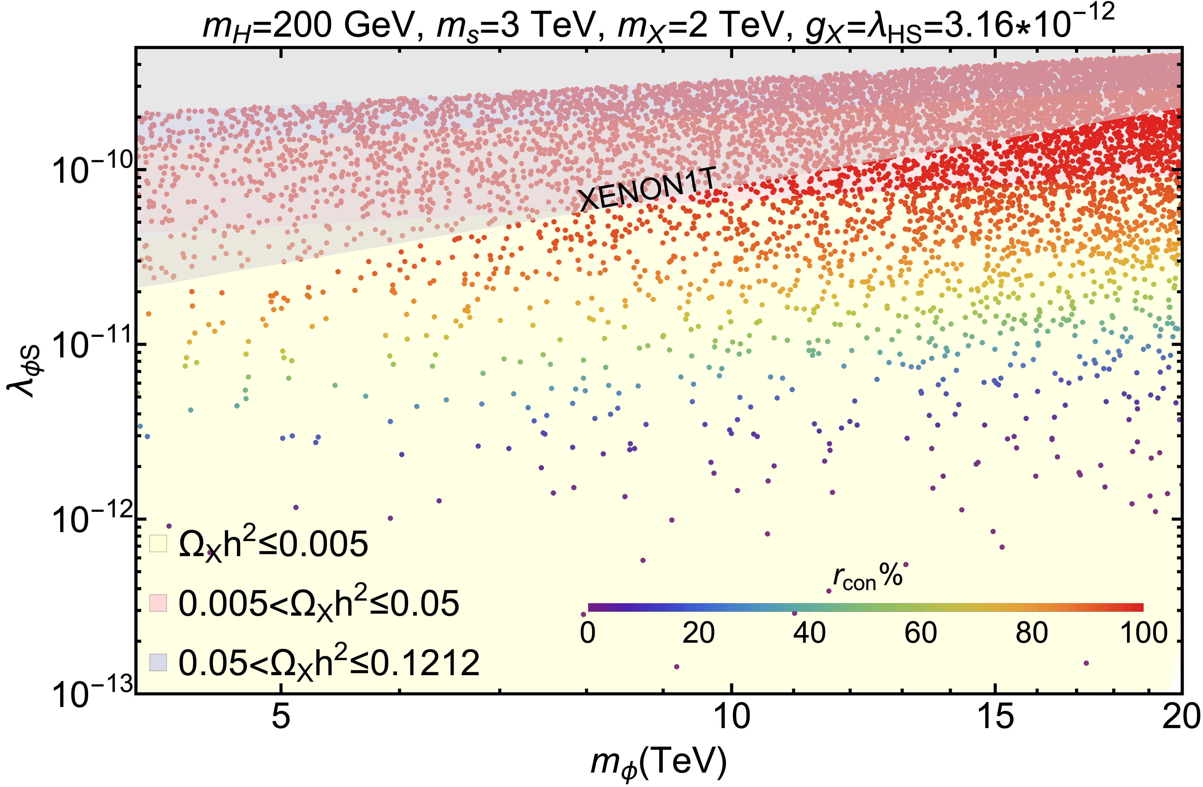
(a)

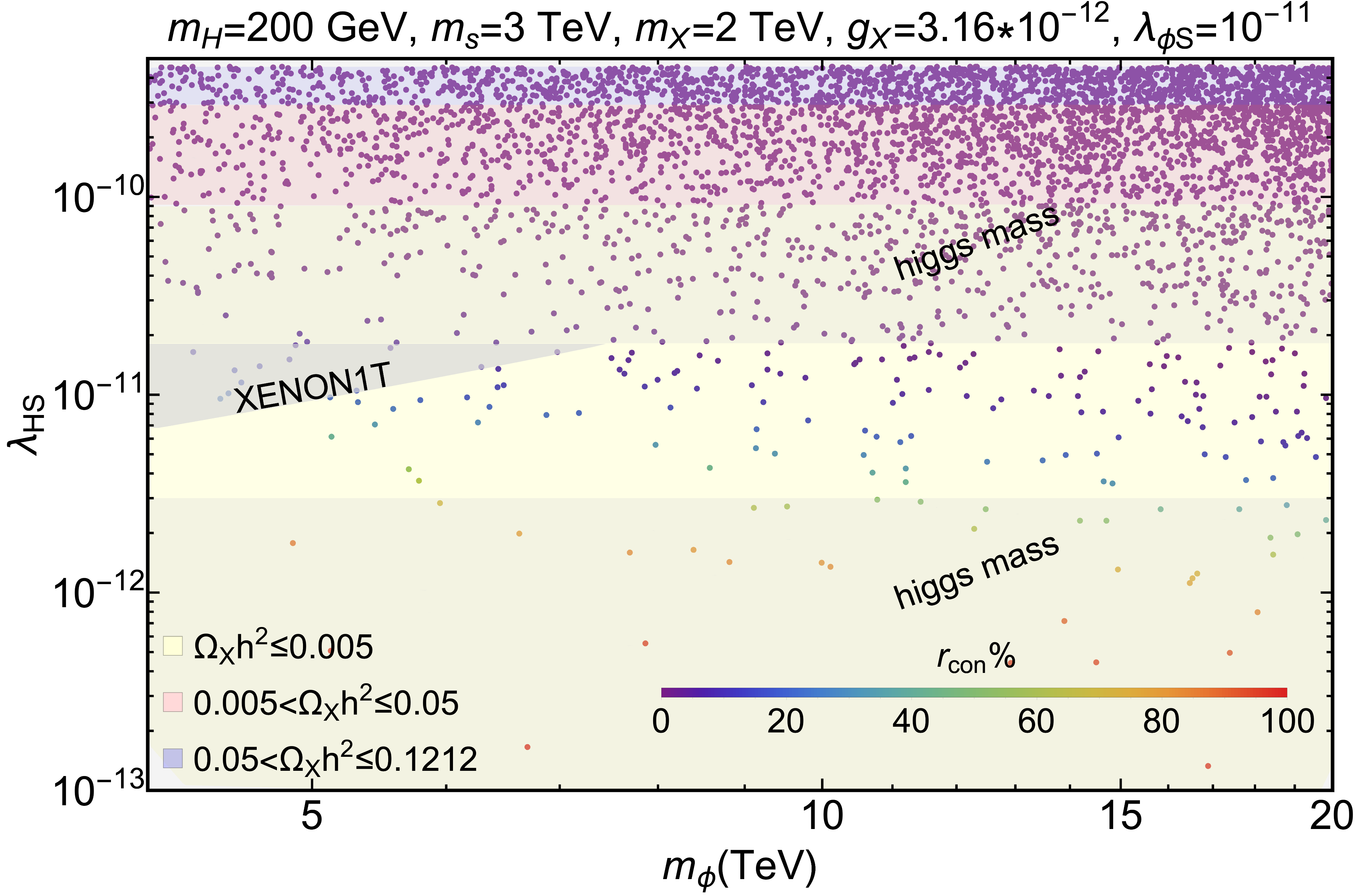
(b)

Figure 10: Numerical scan of the under-abundant region of $X$ relic for freeze-in bEWSB, when $m_{s}<2m_{X}$. Fig. 10a and 10b show correlation in $m_{\phi}-\lambda_{\phi S}$ and $m_{\phi}-\lambda_{HS}$ planes respectively. Three different colour shades indicate different ranges of relic density (see figure inset) for fixed values of other parameters written in figure heading. The rainbow colour bar represents how much the WIMP-FIMP conversion ($\phi\phi\to XX$) is contributing in production of $X$ by the ratio $r_{\rm{con}}$ (see Eq. 36). Grey shaded areas signify the regions excluded by direct detection and Higgs mass constraints.

We turn next to the parameter space scan for the FIMP under abundance in the kinematic region $m_{s}<2m_{X}$ as shown in Fig. 10, correlating different parameters relevant for scattering/conversion processes. While the light yellow, light red and the light blue shaded regions signify different ranges of relic density (see figure inset), the scattered points with different colours as in the colour bar signify the percentage of WIMP-FIMP conversion channels with respect to the total FIMP production via the following ratio:

$$r_{\rm{con}}=\frac{\langle\sigma\mathpzc{v}\rangle_{\phi\phi\to XX}}{\langle\sigma\mathpzc{v}\rangle_{\rm{Tot}}}\,.$$ (36)

As mentioned before, the presence of $s$ after EWSB, when FIMP production is prohibited from the decay of $s$, ensures direct search and collider search possibilities of the model, which in turn puts appropriate bounds on the parameter space in absence of a signal. These constraints are superimposed on the parameter space by grey shaded exclusion regions. Fig. 10a shows scan in $m_{\phi}-\lambda_{\phi S}$ plane and we see that XENON1T bound heavily constrains $\lambda_{\phi S}\lesssim 2\times 10^{-11}$. WIMP-FIMP conversion is then restricted significantly as $\lambda_{\phi S}$ affects conversion contribution directly and FIMP becomes heavily under abundant $\Omega_{X}h^{2}\lesssim 0.005$. In Fig. 10b we show scan in $m_{\phi}-\lambda_{HS}$ plane. As expected Higgs mass bound plays a crucial role together with DD constraints to limit $3\times 10^{-12}\lesssim\lambda_{HS}\lesssim 2\times 10^{-11}$, again to make the FIMP heavily under abundant ($\Omega_{X}h^{2}\lesssim 0.005$), particularly with the choice of $\lambda_{\phi S}=10^{-11}$ as done for the scan. The conversion contribution is large when $m_{\phi}$ is small, as expected.

We further intend to highlight that in all these scans, the parameters directly affecting Higgs mass and mixing after EWSB, ie, $m_{s}$, $m_{X}$ and $g_{X}$ (see Eq. LABEL:eq:mixing) are all very fined-tuned. Owing to this requirement, there is not enough range to show the variations of these parameters in a scan. Therefore, we choose to vary the parameters in the dark sector that does not affect Higgs mass; $\lambda_{HS}$ being the only exception, shows a very narrow viable region, as pointed out in Fig. 10b.

4.6 Freeze-out of $\phi$

The scalar singlet dark matter $\phi$ is assumed to be in thermal bath as WIMP, tracking the equilibrium (non-relativistic and Maxwell-Boltzmann) distribution in early universe. When the bath temperature ($T$) goes below the decoupling temperature of $\phi$, i.e. $T\lesssim T^{\phi}_{D}$, the interaction rate of DM with the bath particles eventually becomes less than the Hubble expansion rate $H$. This causes the DM to decouple from the thermal bath and freeze out to give the saturation abundance. In this section, we assume the freeze-out to occur bEWSB and find the region of parameter space where it happens and produces under abundance. As mentioned previously, there are several constraints to ensure freeze-out bEWSB such as $m_{\phi}\geq$4 TeV. Further constraints on model parameters come from DD and collider searches as discussed before. We indicate the bounds in resulting parameter space. The annihilation channels of WIMP $\phi$, through which it depletes the number density can be divided into two main categories:

• Annihilation to visible sector:

  The channels bEWSB, include $\phi$ pair-annihilation into $s$ and $H$ pairs. The relevant Feynman diagrams are in Fig. 5. The couplings relevant to the above scatterings are $\lambda_{\phi S}$, $\lambda_{HS}$, $\lambda_{\phi H}$ and $\lambda_{S}~{}(=\frac{m_{s}^{2}}{2v_{s}^{2}})$. As already mentioned, $v_{s}=m_{X}/g_{X}$ must always be very large ( $\sim 10^{14}$ GeV) throughout the analysis in order to have a successful FIMP ($X$) production as a CDM. Hence, unless we choose $\lambda_{\phi S}\sim 1/v_{s}$, couplings like $\phi\phi s\ (\propto v_{s}\lambda_{\phi S}$), will make the annihilation cross-sections very large, resulting in negligible $\phi$ abundance. Hence, in order to get a reasonable annihilation of $\phi$,

  $$\lambda_{\phi S}\lesssim 10^{-12}~{}{\rm for}~{}g_{X}\sim 10^{-12}.$$

  Such a choice is consistent with both the freeze-in of $X$ and direct detection constraints on $\lambda_{\phi S}$. Although such small $\lambda_{\phi S}$ makes the four-point scattering cross section, such as the top left channel in Fig. 5, practically negligible, $\phi$ mainly annihilates via the $s$ and $t$-channel diagrams in Fig. 5, where presence of $v_{s}$ in one of the vertices like $\phi\phi s$ make the contribution sizeable. We further note that $\lambda_{\phi H}$ should also be greater than $10^{-3}$ to get a reasonable annihilation via $\phi\phi\to HH$. Although $\phi$ freezes out bEWSB, we recall that $s$ and $h$ mixes due to EWSB. As a result, $\lambda_{HS}$ is traded off as a parameter dependent on mixing. So, the collider searches of Higgs at the LHC, restricts $\lambda_{HS}$. We indicate the effect of such constraints on the allowed parameter space.

• Conversion to FIMP DM :

  $\phi$ annihilates into $X$ pair via $s$ mediation (bottom panel of Fig. 5). But since freeze-in requires $g_{X}$ to be very small ($\lesssim 10^{-12}$), one vertex of conversion diagram ($XXs$) proportional to $g_{X}^{2}v_{s}$ is also minuscule; this evidently implies that unless the other vertex $\lambda_{\phi S}$ is chosen sufficiently large ($\sim$ 1), the conversion contribution is negligible. However, $\lambda_{\phi S}$ requires to be small from DD, makes the conversion very small. Secondly, large conversion cross section to FIMP production automatically implies that $X$ production will be too fast for the non-thermal freeze-in and it will drive $X$ towards equilibrium, seizing the FIMP nature of $X$. Hence, WIMP$\leftrightarrow$FIMP conversion is negligible in the context of WIMP, but plays an important role in the FIMP production as already demonstrated in previous subsection.

Upon neglecting the WIMP-FIMP conversion, the cBEQ reduces to two individual uncoupled BEQs; the one for $\phi$ is given by Eq. 29, which can be easily solved numerically (we use Mathematica 12.3.1.0 Mathematica ). The parameters are chosen in such a way that the freeze-out occurs bEWSB. The relic density for $\phi$ can then be written in terms of freeze-out yield Kolb:1990vq and we again focus on the under abundant region of the parameter space, given $\phi$ is one of the two DM components that we assume to constitute the dark sector:

$$\Omega_{\phi}{\rm h^{2}}\simeq 2.744\times 10^{8}\ m_{\phi}Y_{\phi}^{{\rm bEWSB}};~{}~{}\Omega_{\phi}{\rm h^{2}}\leq 0.1212\,.$$

where WIMP dark matter relic density is written in terms of the reduced Hubble parameter, $h$ in units of 100 km/s/Mpc.

4.6.1 Phenomenology

We first study $\phi$ freeze-out bEWSB as a solution of the BEQ 29 in Fig. 11, where we plot $\Omega_{\phi}h^{2}$ with $x=m_{\phi}/T$ for parameters $\lambda_{HS},\lambda_{\phi S},m_{\phi},g_{X}$. We choose three representative values of these parameters so that we produce correct relic, under abundance and over abundance. The horizontal black dotted line denotes the current central value of DM abundance. Vertical dot-dashed lines indicate EWSB ($x_{\rm{EW}}={m_{\phi}}/{160~{}\rm{GeV}}$) and each freeze out occurs bEWSB with $x_{\rm{FO}}<x_{\rm{EW}}$. The parameters kept fixed for these plots, as mentioned in the figure insets and headings, comply with all the constraints mentioned earlier.

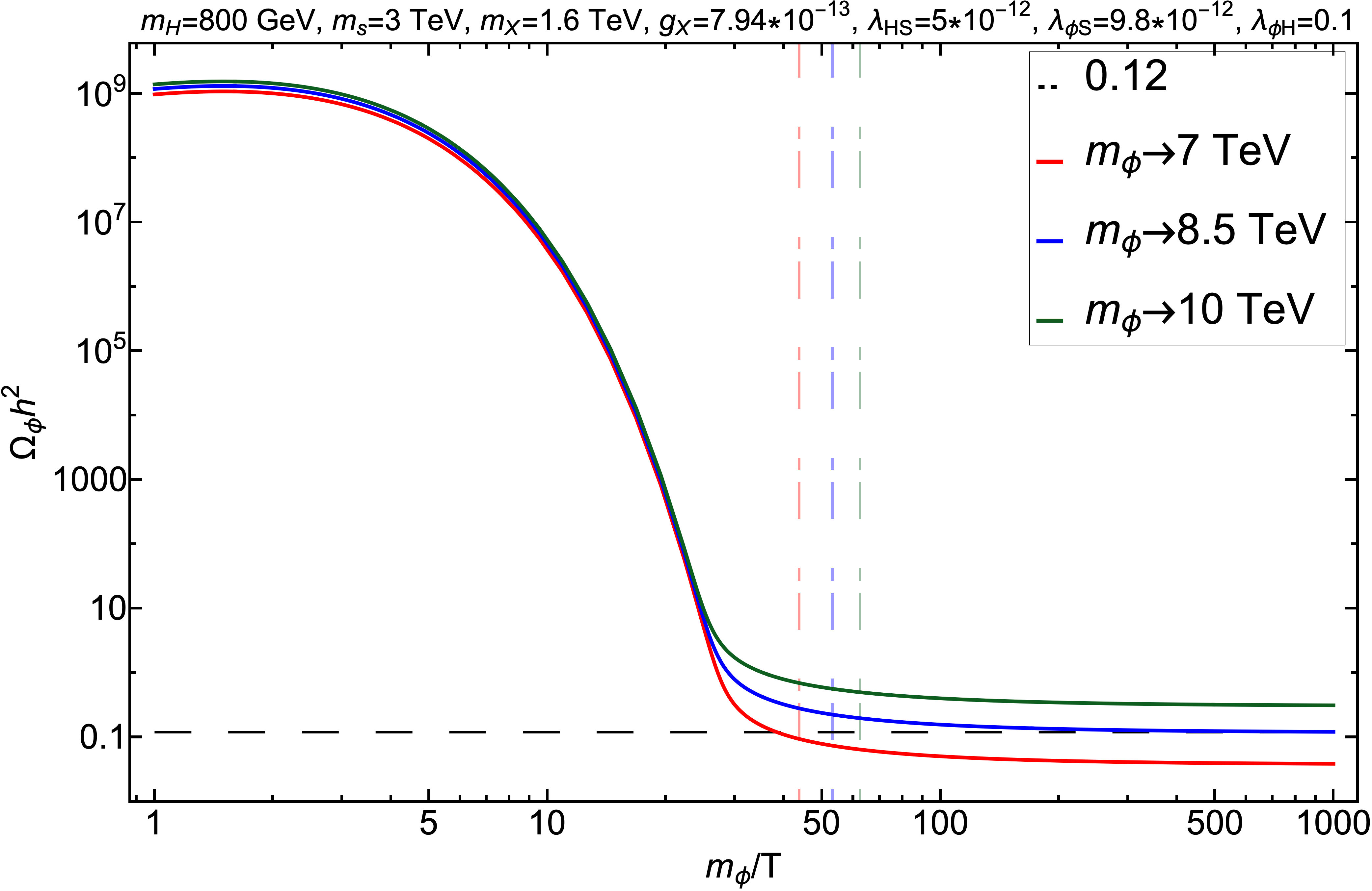
(a)

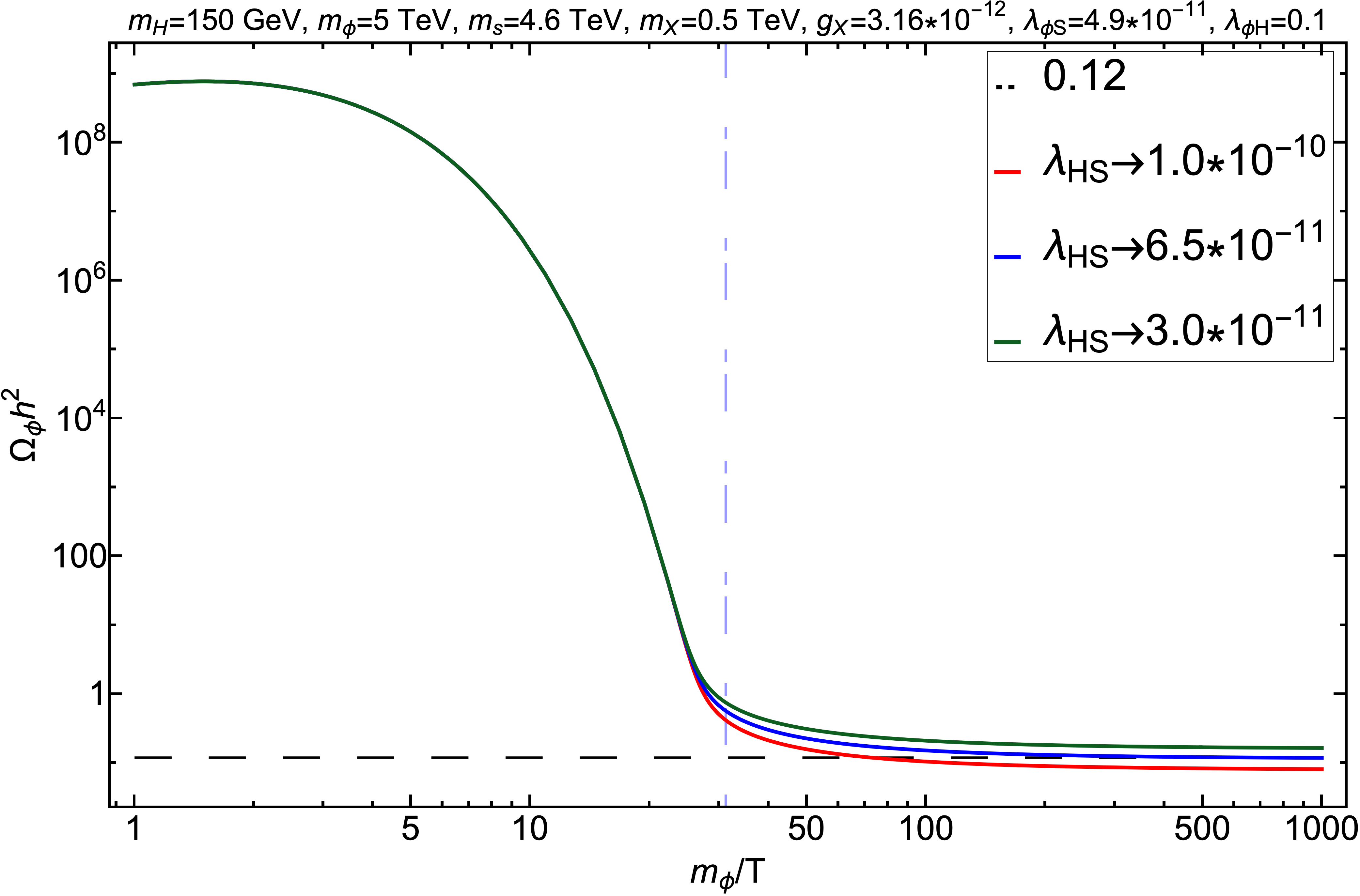
(b)

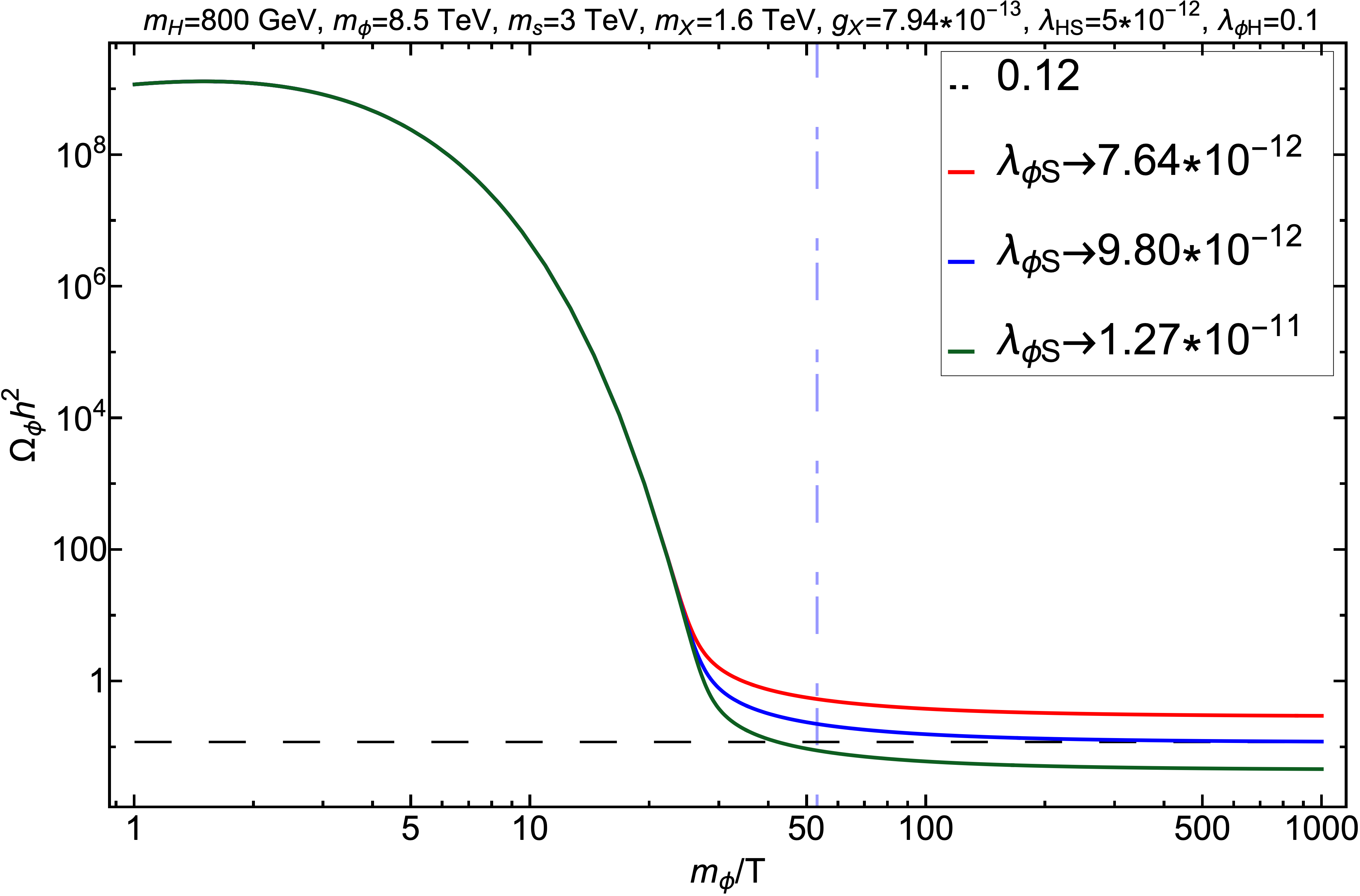
(c)

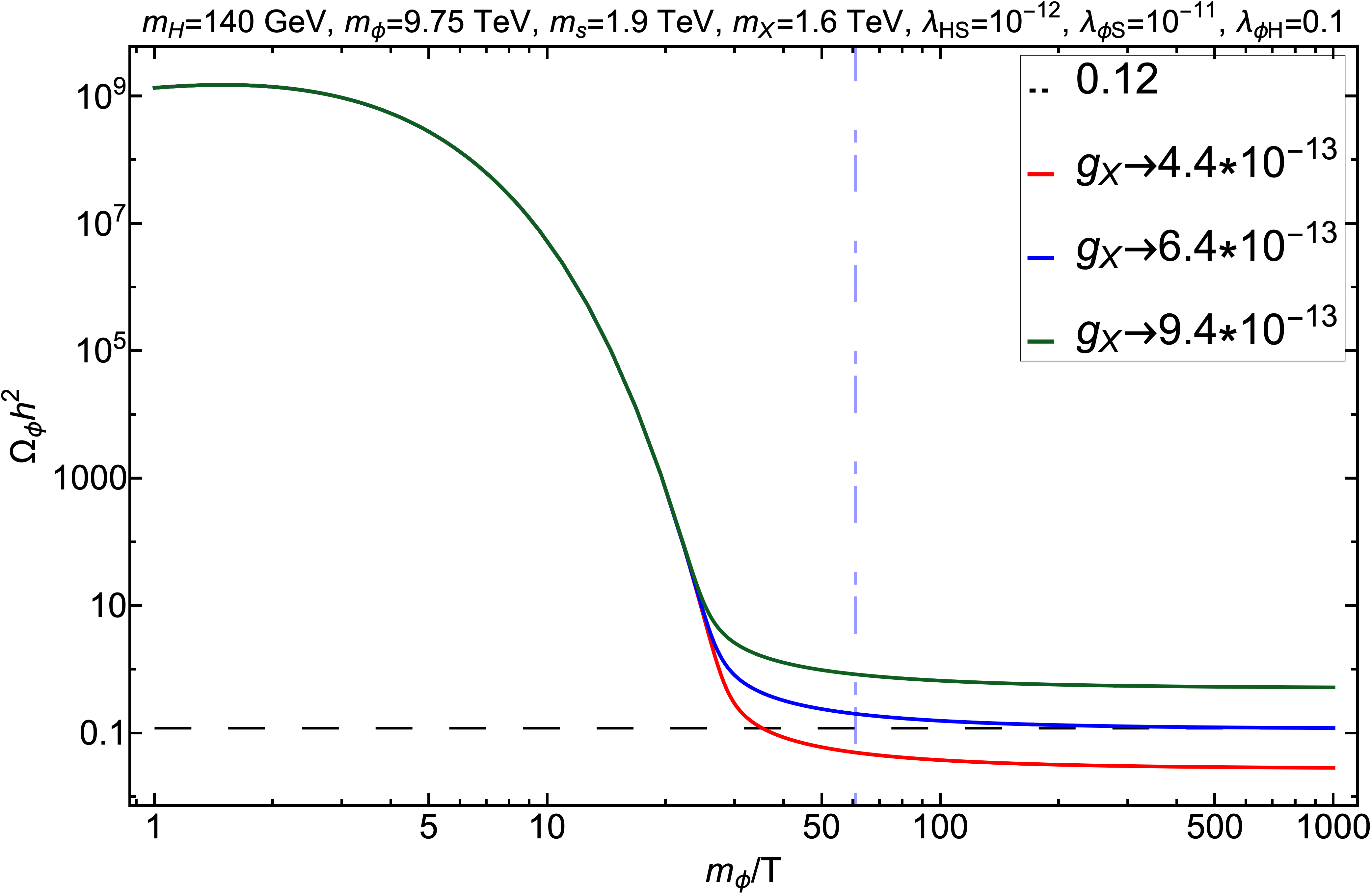
(d)

Figure 11: WIMP relic density ($\Omega_{\phi}h^{2}$) in terms of $x=m_{\phi}/T$ for three different values of parameters $\lambda_{HS},\lambda_{\phi S},m_{\phi},g_{X}$ (from left to right and top to bottom) to provide correct relic, under and over abundance. The parameters kept fixed are mentioned in the insets as well as in the figure headings. The horizontal black dotted line denotes correct relic abundance and the vertical dot-dashed lines depict EWSB, $x_{\rm{EW}}=m_{\phi}/160$.

As already mentioned, to ensure the WIMP freeze-out to take place bEWSB, the allowed mass of $\phi$ is constrained to $m_{\phi}\gtrsim 4$ TeV. To comply with this bound, in Fig. 11a, the freeze out of $\phi$ is shown for $m_{\phi}=$ 7 TeV, 8.5 TeV and 10 TeV, depicted by red, blue and green coloured lines respectively. As annihilation cross-section is inversely proportional to WIMP mass, and freeze-out yield is also inversely proportional annihilation cross-section, we see that as $m_{\phi}$ increases, the WIMP relic density also enhances and the case with $m_{\phi}=8.5$ TeV matches with correct relic. In Figs. 11b, 11c and 11d, we show the effects in WIMP relic due to variation of $\lambda_{HS},\lambda_{\phi S},g_{X}$ respectively. As the annihilation cross-section of WIMP ($\phi$) increases with larger couplings, we see that the relic density reduces expectedly with larger $\lambda_{HS},\lambda_{\phi S}$ in Fig. 11b and 11c. The scenario changes in Fig. 11d, where variation with respect to $g_{X}$ is shown. In annihilation cross-section, $g_{X}$ enters inversely through $v_{s}~{}(=m_{X}/g_{X})$, as a result, annihilation to $H,s$ reduces with the increase of $g_{X}$, resulting in an enhancement of relic with $g_{X}$ as shown in Fig. 11d.

DD of $\phi$ occurs through Higgs mediation (see Appendix D). Even if WIMP freezes-out bEWSB, direct search of $\phi$ is possible at present epoch, so the constraints apply. However, the constraints depend on kinematical regions: (i) $m_{s}\geq 2m_{X}$ and (ii) $m_{s}<2m_{X}$ in a similar vein as discussed before.

Case-I: $\left(m_{s}\geq 2m_{X}\right):$

When $m_{s}\geq 2m_{X}$, and we ensure $X$ freeze-in to saturate bEWSB, the decay of $s$ totally depletes its number density, so that any $s-h$ mixing aEWSB is non-existent, resulting only SM Higgs mediating direct search for $\phi$. So the situation is similar to the DD of single component scalar singlet $\phi$.

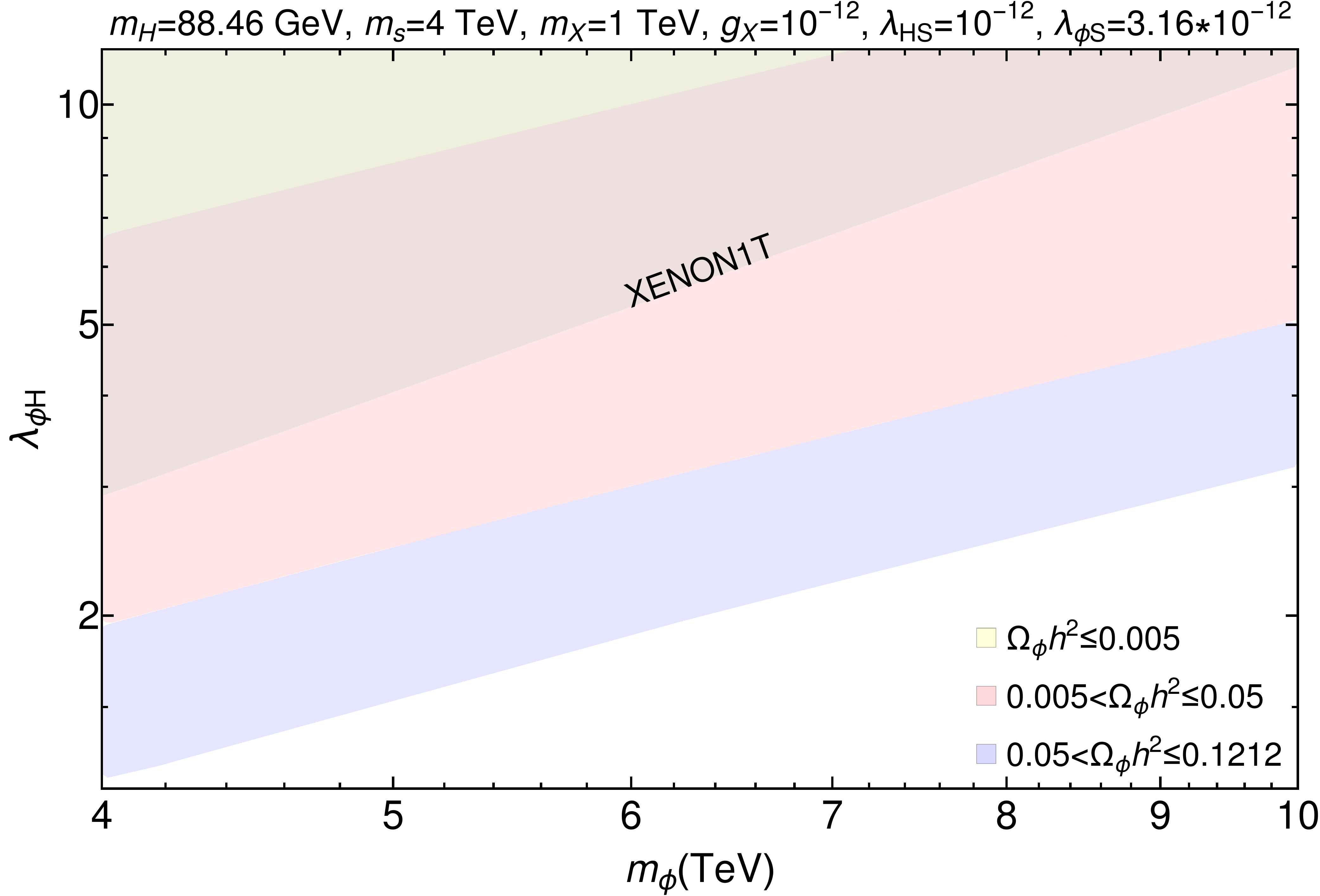
Figure 12: Under abundant region for $\phi$ ($\Omega_{\phi}\rm h^{2}\leq 0.1212$) with respect to variation of $\lambda_{\phi H}$ vs. $m_{\phi}$ for kinematic region $m_{s}\geq 2m_{X}$ when freeze-out occurs bEWSB. Spin independent XENON1T direct search excluded region is showed by the grey shaded area at the top for large $\lambda_{\phi H}$. Light yellow, light red and light blue shades indicate different ranges of $\Omega_{\phi}\rm h^{2}$ as mentioned in figure inset. Parameters kept fixed for the plot are mentioned in the figure heading and comply with all other constraints.

Fig. 12 shows the under abundant parameter space in $m_{\phi}-\lambda_{\phi H}$ plane where $\phi$ freezes out bEWSB, in the kinematic region $m_{s}\geq 2m_{X}$. Three colour shades indicate different ranges of $\Omega_{\phi}h^{2}$ (mentioned figure inset). The grey shaded region is excluded by the present spin-independent XENON1T limit, which restricts only very high values of $\lambda_{\phi H}\gtrsim 3$, given other parameters are kept constant at values mentioned in the figure heading. As $m_{s}>4$ TeV (see Eq. 33) for late decay to complete bEWSB, WIMP annihilation mostly occur through the four point interaction $\phi\phi\to HH^{\dagger}$. The correlation between $m_{\phi}-\lambda_{\phi H}$ is consistent with two features already discussed: (a) WIMP annihilation cross-section via four point interaction increases with $\lambda_{\phi H}$ which in turn reduces the abundance and (b) WIMP annihilation cross-section decreases with $m_{\phi}$, which causes $\Omega_{\phi}h^{2}$ to increase with the WIMP mass.

Case-II: $\left(m_{s}<2m_{X}\right):$

When $m_{s}\leq 2m_{X}$, $s-h$ mixing occurs aEWSB and direct search occurs via mediation of both physical states $h_{1},h_{2}$. Therefore, mixing plays an important role in the direct detection of WIMP. In this case, the parameter space and the constraints are expectedly different from the previous case where mixing was absent. Correlations of relevant parameters for under abundance of $\phi$ ($\Omega_{\phi}\rm h^{2}\leq 0.1212$) in this kinetic regime is shown in Fig. 13 together with direct search and Higgs mixing constraint.

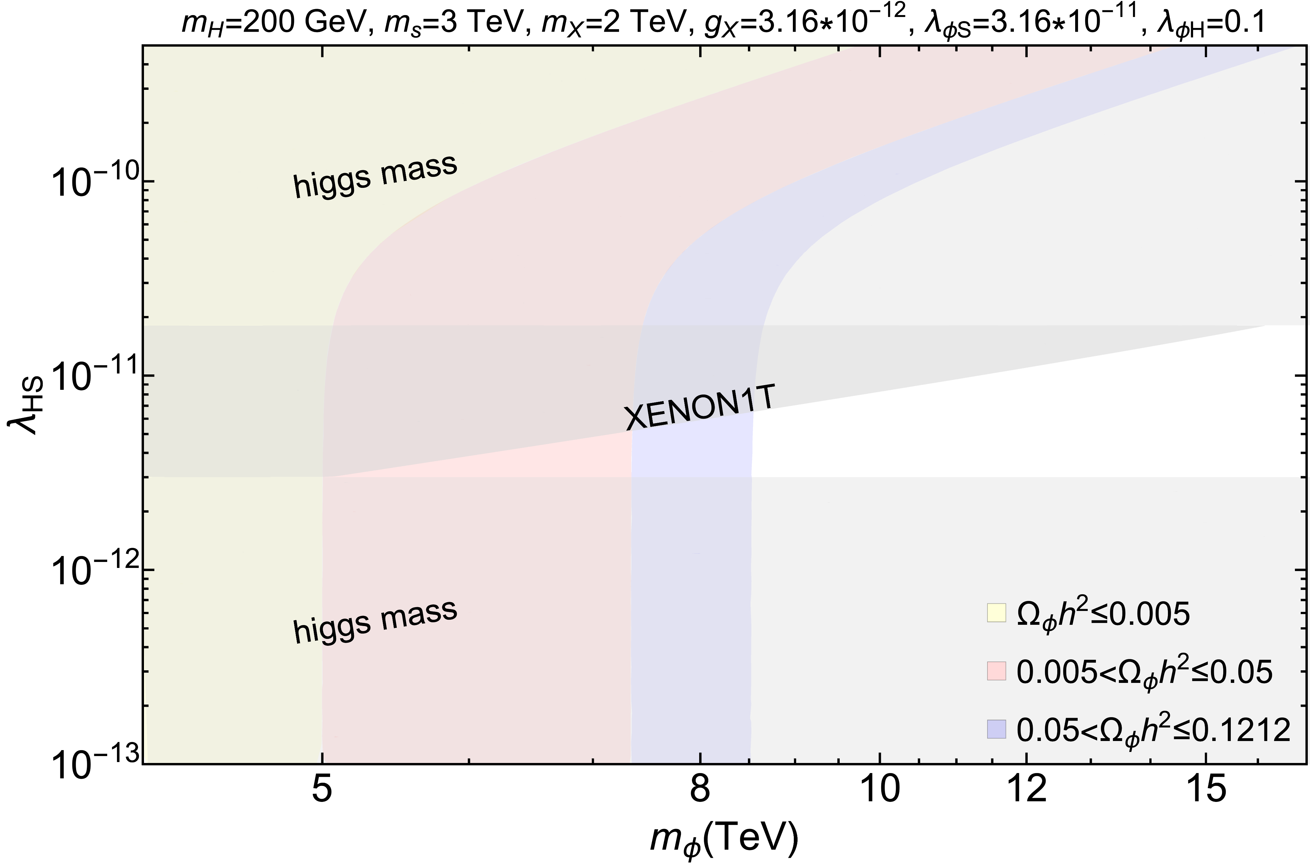
(a)

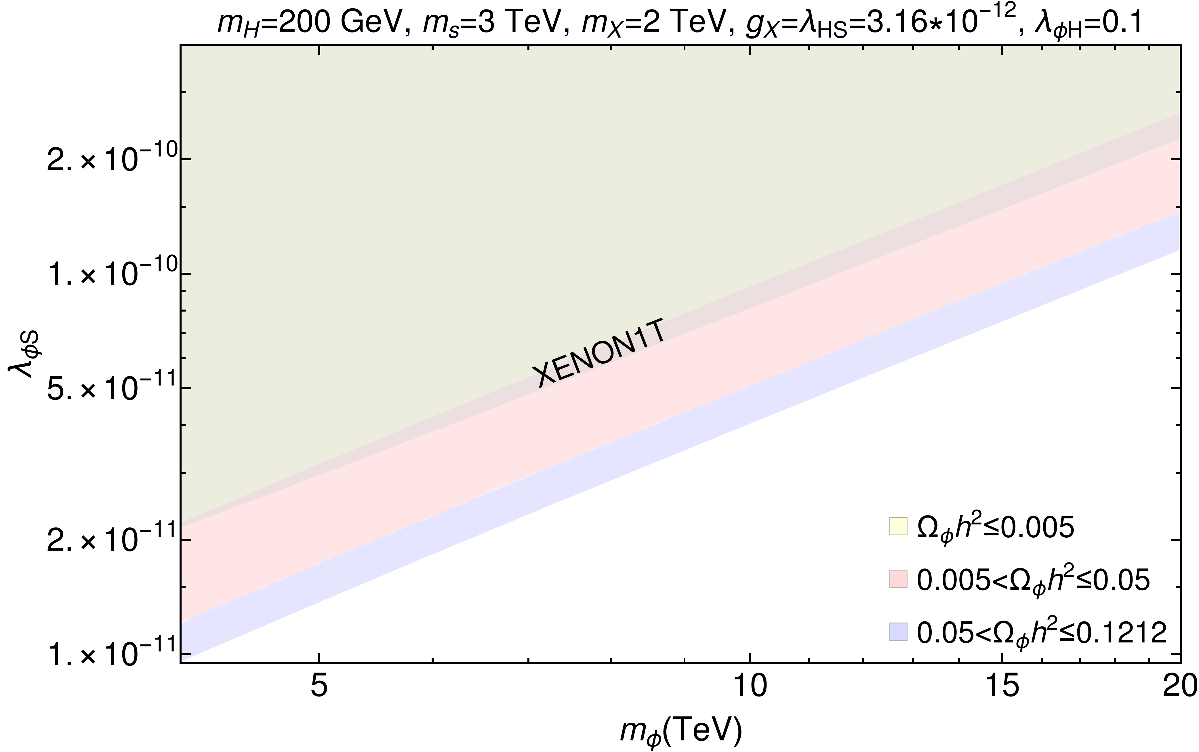
(b)

Figure 13: Under abundance for $\phi$ ($\Omega_{\phi}\rm h^{2}\leq 0.1212$) in the kinematic region $m_{s}<2m_{X}$. Fig. 13a shows the correlation between $m_{\phi}-\lambda_{HS}$ and Fig. 13b shows the correlation between $m_{\phi}-\lambda_{\phi S}$. Different colour shades in light yellow, light red and light blue indicates under abundance within ranges as mentioned in figure inset. Grey shaded regions are excluded by latest XENON1T bound, Higgs mass and collider bound on scalar mixing (see text for details).

Fig. 13a shows the under abundant parameter space in $m_{\phi}$ vs. $\lambda_{HS}$ plane where grey shaded regions are excluded by XENON1T direct search bound and Higgs mass/scalar mixing constraints. The functional dependence of $m_{\phi}$ as in Fig. 11a and of $\lambda_{HS}$ as in Fig. 11b are retained here. We conclude that $\lambda_{HS}\sim 5\times 10^{-12}$ is safe for $m_{\phi}$ varying within 7 to 8.5 TeV, given the other model parameters are kept fixed as mentioned in the figure caption. Fig. 13b shows the correlation between $m_{\phi}-\lambda_{\phi S}$. Recall that $Y_{\phi}$ increases with larger $\lambda_{\phi S}$ (see Fig. 11c) as well as with larger WIMP mass ($m_{\phi}$), which is also evident in Fig. 13b. Once $\lambda_{HS}\sim 3.16\times 10^{-12}$ is fixed in Fig. 13b, it fixes the mixing angle within experimental limit, there is no other constraint on this parameter space excepting for the direct search bounds, depicted in grey shade.

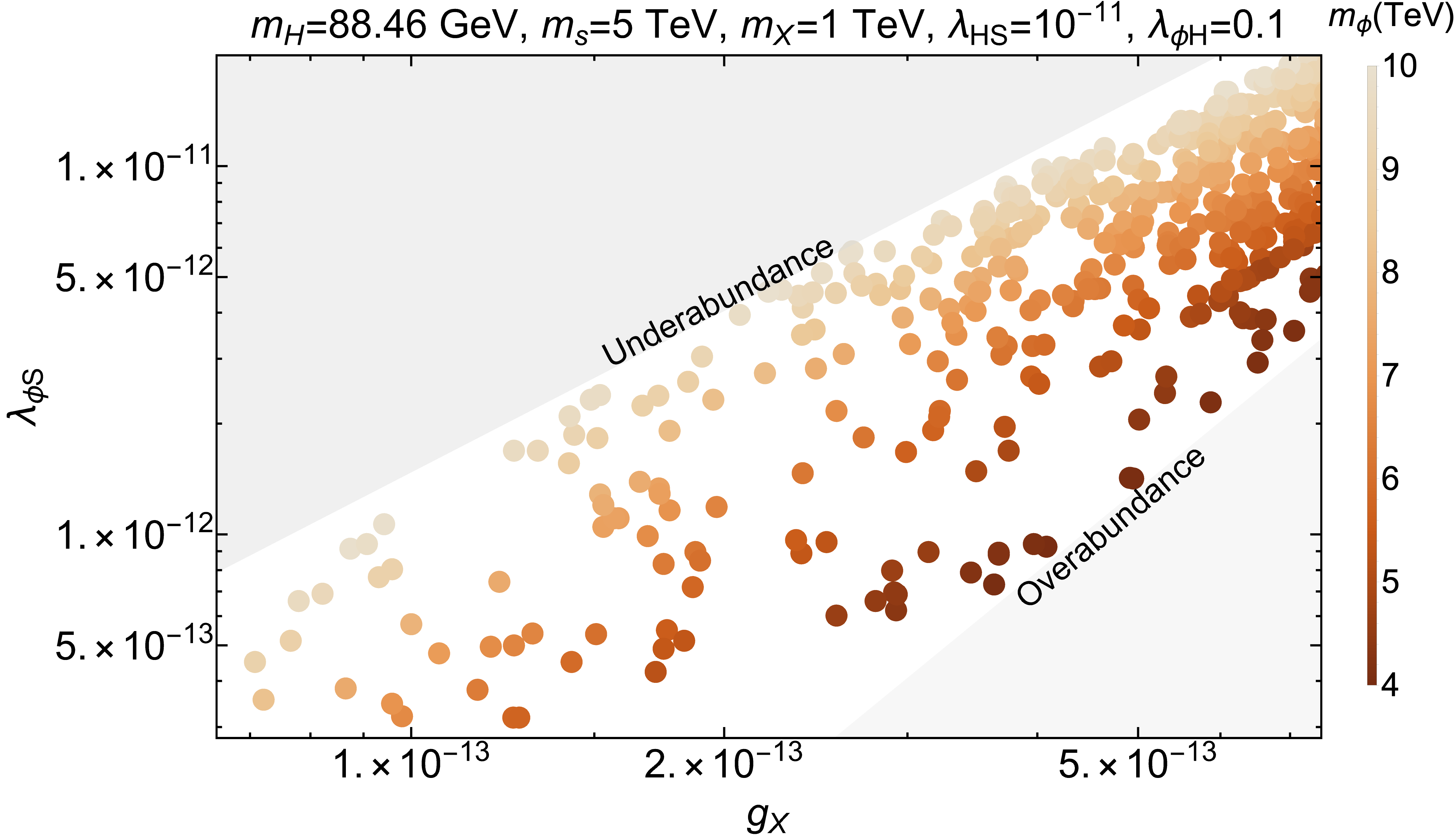
(a)

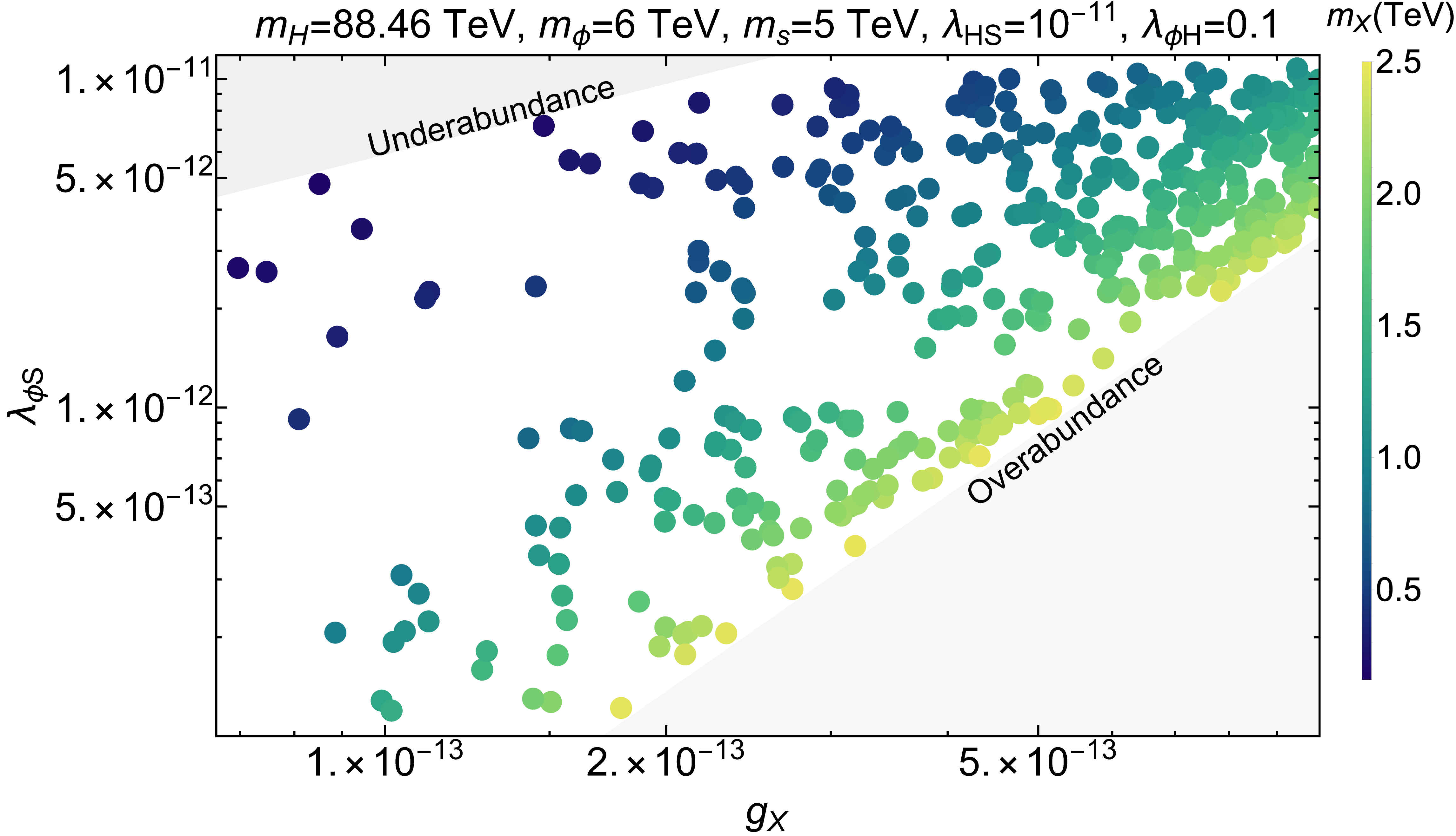
(b)

Figure 14: Scan in $g_{X}-\lambda_{\phi S}$ plane when both WIMP and FIMP components add to observed relic density, $\Omega_{X}h^{2}+\Omega_{\phi}h^{2}=0.1200\pm 0.0012$, simultaneously addressing other constraints when both freeze in and freeze out occur bEWSB in kinematic region $m_{s}\geq 2m_{X}$. In Fig. 14a, we keep FIMP mass fixed at $m_{X}=1$ TeV and vary WIMP mass $m_{\phi}$ as shown in the SiennaTones colour bar. In Fig. 14b, we keep $m_{\phi}=6$ TeV fixed and vary $m_{X}$ as shown by the BlueGreenYellow colour bar. Other parameters kept fixed are mentioned in the figure heading.Under abundance and over abundance constraints from freeze-in/freeze-out bEWSB are shown by grey shaded regions.

4.7 Putting WIMP and FIMP together

Scenario	Benchmark    points	$m_{H},m_{\phi},m_{s},m_{X}$       (TeV)	$g_{X},\lambda_{HS},\lambda_{\phi S},\lambda_{\phi H}$	$\Omega_{\phi}h^{2}$	$\Omega_{X}h^{2}$	$\frac{\Omega_{\phi}}{\Omega_{T}}\%$	$\frac{\Omega_{X}}{\Omega_{T}}\%$	$\sigma_{\phi_{eff}}^{\text{SI}}$ $(\text{cm}^{2})$
$m_{s}\geq 2m_{X}$	BP1	0.088, 8.0, 7.0, 1.0	$10^{-13},10^{-11},5.69\times 10^{-13},0.1$	0.1176	0.0014	98.82	1.18	$1.44\times 10^{-48}$
	BP2	0.088, 7.0, 6.0, 1.5	$10^{-12},10^{-11},1.07\times 10^{-11},0.1$	0.0626	0.0571	52.30	47.70	$9.99\times 10^{-49}$
	BP3	0.088, 6.0, 5.0, 2.0	$2.33\times 10^{-12},10^{-11},2.6\times 10^{-11},0.1$	0.0087	0.1112	7.26	92.74	$1.89\times 10^{-49}$
$m_{s}<2m_{X}$	BP4	0.2, 8.3, 3.0, 2.0	$10^{-11},10^{-11},10^{-10},0.3$	0.1062	0.0138	88.50	11.50	$2.05\times 10^{-45}$
	BP5	0.2, 14.5, 3.0, 2.0,	$10^{-11},10^{-11},2.74\times 10^{-10},0.3$	0.0592	0.0605	49.46	50.54	$3.09\times 10^{-45}$
	BP6	0.2, 11.0, 3.0, 2.0	$10^{-11},10^{-11},3.32\times 10^{-10},0.2$	0.0056	0.1154	4.63	95.37	$7.55\times 10^{-46}$

Table 3: Some sample benchmark points for the WIMP-FIMP model, when both freeze-in of $X$ and freeze-out of $\phi$ occur bEWSB respecting the total relic density, direct search, Higgs mass/mixing and other constraints. The benchmark points depict the possibilities when one component dominates over the other as well as the case when they have almost equal share for the total DM relic density.

So far we discussed the under abundant parameter space for both WIMP ($\phi$) and FIMP ($X$) individually when they freeze-out and freeze-in bEWSB. However, the fact that the total DM relic density has to be achieved (Eq. 21) from both these components, will correlate these two cases. Two such example scans are shown in Fig. 14, where we show the relic density allowed parameter space in $\lambda_{\phi S}-g_{X}$ plane for the kinematic region $m_{s}\geq 2m_{X}$, abiding by other relevant constraints. In Fig. 14a, we keep FIMP mass fixed at $m_{X}=1$ TeV and vary WIMP mass $m_{\phi}$ as shown in the SiennaTones colour bar. In Fig. 14b, we keep $m_{\phi}=6$ TeV fixed and vary $m_{X}$ as shown by the BlueGreenYellow colour bar. The other parameters kept fixed are mentioned in the figure headings.

In Fig. 14a, we see that for a fixed $g_{X}$, when we make $\lambda_{\phi S}$ larger, the FIMP ($X$) relic almost remains the same, but WIMP ($\phi$) relic decreases due to larger annihilation cross-section; so $m_{\phi}$ requires to be larger to keep the WIMP relic in the similar ballpark and total relic density constant. This is why we see darker points with smaller $m_{\phi}$ populating smaller $\lambda_{\phi S}$ regions, while for larger $\lambda_{\phi S}$, the WIMP mass( $m_{\phi}$) requires to be larger with brighter points populating such regions. In the same figure, we see that when we enhance $g_{X}$, FIMP relic gets larger, and accordingly WIMP relic needs to be smaller by having larger $\lambda_{\phi S}$ as well as small $m_{\phi}$. Of course, if we keep $\lambda_{\phi S}$ unchanged with larger $g_{X}$, the total relic density goes beyond the experimental observation and provides over abundance, shown by grey shaded region. In a similar way, when $\lambda_{\phi S}$ is larger than a specific value for a given $g_{X}$, then WIMP relic is so tiny that it leads to under abundant total relic, also marked by the grey shaded region. A complementary behaviour is observed in Fig. 14b. Here, for a fixed $g_{X}$, with larger $\lambda_{\phi S}$, WIMP relic decreases, but with $m_{\phi}$ kept constant, there is only one way to keep the observed relic density constant, by enhancing FIMP contribution i.e. by decreasing $m_{X}$. This is why we see darker points with small $m_{X}$ favouring larger $\lambda_{\phi S}$ regions and brighter points with larger $m_{X}$ populating smaller $\lambda_{\phi S}$ regions. Grey shaded over abundance for small $\lambda_{\phi S}$ and under abundance for large $\lambda_{\phi S}$ regions can be described in a similar way as in Fig. 14a. A similar correlation can be made when FIMP production occurs dominantly via scattering processes with $m_{s}\leq 2m_{X}$, but the allowed parameter space becomes tinier due to the involvement of $\lambda_{\phi S}$ into both freeze-in and freeze-out processes. We next furnish some characteristic benchmark points in Table 4.7, where the abundance of FIMP ($X$) and WIMP ($\phi$) adds to the total observed relic density together with addressing direct search and Higgs mixing constraints ensuring that freeze-in of $X$ and freeze-out of $\phi$ both occur bEWSB. The benchmark points BP1 and BP4 depict the possibilities when $\phi$ dominates over $X$, BP3, BP6 show the other possible hierarchy when $X$ dominates over $\phi$, while BP2 and BP5 demonstrate the case when they have almost equal share for the relic density. Before concluding this section, we would like to comment that if both freeze-in/freeze-out has to occur bEWSB the masses $m_{\phi},m_{s}$ need to be very heavy, and possibility of any collider production is difficult. The FIMP is anyway very feebly coupled to SM. The WIMP can still have a direct search possibility, larger when the FIMP can be produced via scattering, smaller when it is produced via $s\to XX$ decay, providing an interesting correlation between the WIMP and FIMP DM components.

5 Dark Matter phenomenology aEWSB

In this section, we address a situation where the freeze-in of $X$ and freeze-out of $\phi$ both occur after EWSB. This is equivalent to saying that both the DM components attain saturation at a temperature smaller than $T_{\rm{EW}}$, i.e.:

$$T_{U(1)}>T_{\rm{EW}}>T_{\rm{FI}};~{}~{}T_{U(1)}>T_{\rm{EW}}>T_{\rm{FO}}\,.$$ (37)

The methodology of finding the allowed parameter space for such a situation is similar to the previous case; to solve BEQ for both WIMP and FIMP cases individually including all the processes that contribute aEWSB, and choosing model parameters in such a way that we satisfy Eq. 37. This is the case usually considered for most of the DM analysis, excepting for checking the validity of Eq. 37, which we additionally ensure. However, as the approach remains the same as elaborated in the last section, we highlight on the main features that this possibility offers, without going too much of the details.

5.1 Physical states and interactions

The physical particles and interactions aEWSB is obtained when both $S$ and $H$ acquire non-zero VEVs $v_{s}$ and $v$ respectively. In unitary gauge we write,

$$S=\frac{v_{s}+s}{\sqrt{2}}\to\langle S\rangle=\frac{1}{\sqrt{2}}v_{s},~{}H=\begin{pmatrix}0\\ \frac{h+v}{\sqrt{2}}\end{pmatrix}\to\langle H\rangle=\frac{1}{\sqrt{2}}v,~{}\langle\phi\rangle=0\,.$$ (38)

Evidently, this induces mixing between the two scalars ($s-h$), the strength of which is dictated by the mixing angle $\theta$. Upon diagonalization, two physical scalars $h_{1}$ and $h_{2}$ emerge, where $h_{1}$ is assumed to be the SM Higgs with $m_{h_{1}}\sim$125.1 GeV, whereas $h_{2}$ may be assumed heavy with mass $m_{h_{1}}\ll m_{h_{2}}$. The physical and the unphysical fields are related through an orthogonal matrix,

$$\begin{pmatrix}h_{1}\\ h_{2}\end{pmatrix}=\begin{pmatrix}\cos\theta&-\sin\theta\\ \sin\theta&\cos\theta\end{pmatrix}\begin{pmatrix}h\\ s\end{pmatrix}\,.$$ (39)

For details, see Appendix LABEL:sec:aEWSB-details, where the minimization of the scalar potential and emergent conditions are specified. We may note one point here that $\lambda_{HS}$, which was an external parameter bEWSB, can now be considered as an internal parameter and it is dictated by the mixing angle as given below:

$$\lambda_{HS}=\frac{\sin 2\theta}{2v_{s}v}\left(m^{2}_{h_{2}}-m^{2}_{h_{1}}\right).$$ (40)

In Table 4, we list all the relevant parameters of the model considered for the analysis, classified into external (parameters that we choose to vary as input) and internal (or derived) parameters. We further note, that excepting for the constraints on dark sector particle masses imposed to make the freeze-in/freeze-out occur bEWSB, we adhere to all the other constraints as in section 4.2.

External parameters	Internal parameters
$m_{h_{1}}$, $m_{\phi}$, $m_{h_{2}}$, $m_{X}$, $g_{X}$, $\lambda_{\phi}$, $\lambda_{\phi S}$, $\lambda_{\phi H}$, $\sin\theta$	$\mu_{H}$, $\mu_{\phi}$, $\mu_{S}$, $v_{s}$, $\lambda_{H}$, $\lambda_{S}$, $\lambda_{HS}$

Table 4: The parameters used in the aEWSB analysis.

We further note here that WIMP mass for $\phi$ aEWSB is changed due to the additional contribution proportional to DM-Higgs portal interaction $\lambda_{\phi H}$. See Eq. 58 in Appendix LABEL:sec:aEWSB-details, where $\mathfrak{m}_{\phi}$ refers to WIMP mass aEWSB, although we have used the same notation $m_{\phi}$ in the text to avoid clutter. This essentially does not affect the phenomenology to a great extent.

5.2 BEQ in aEWSB scenario

The BEQ does not change aEWSB, the change is only in the processes of DM production and annihilation, and in the limit of $x$ which goes beyond $x_{\rm{EW}}$. First point to note that even aEWSB, the WIMP-FIMP conversion is still small to keep $X$ out-of-equilibrium, so that it is only relevant for FIMP production, and the cBEQs reduce to two independent BEQs as before,

$$\begin{split}\frac{dY_{X}}{dx}&=\Biggl{\{}\frac{45}{3.32\pi^{4}}\frac{g_{s}\,{\rm M_{Pl}}\,m_{s}^{2}\Gamma_{s\to XX}}{m_{X}^{4}}\frac{x^{3}K_{1}\left[\frac{m_{s}}{m_{X}}x\right]}{g^{s}_{*}(x)\sqrt{g_{*}^{\rho}(x)}}\\ &+\frac{4\pi^{2}\rm{M_{Pl}}}{45\times 1.66}\frac{g^{s}_{*}(x)}{\sqrt{g^{\rho}_{*}(x)}}\frac{m_{X}}{x^{2}}\left(\sum_{i=s,H}\,\langle\sigma\mathpzc{v}\rangle_{ii\to XX}(Y_{i}^{eq})^{2}+\langle\sigma\mathpzc{v}\rangle_{\phi\phi\to XX}Y_{\phi}^{2}\right)\Biggr{\}}\Theta[x_{\rm{EW}}-x]\\ &+\Biggl{\{}\frac{45}{3.32\pi^{4}}\sum_{A=h_{1},h_{2}}\frac{g_{A}\,{\rm M_{Pl}}\,m_{A}^{2}\Gamma_{A\to XX}}{m_{X}^{4}}\left(\frac{x^{3}K_{1}\left[\frac{m_{A}}{m_{X}}x\right]}{g^{s}_{*}(x)\sqrt{g_{*}^{\rho}(x)}}\Theta[x_{D}^{A}-x]\right.\\ &\left.+\ e^{-\frac{0.602\,{\rm M_{Pl}}\,\Gamma_{A\to XX}}{m_{X}^{2}\sqrt{g^{\rho}_{*}(x)}}(x^{2}-x_{D}^{A^{2}})}\frac{x^{2}x_{D}^{A}}{\eta(x,x_{D}^{A})}K_{1}\left[\alpha(x,x_{D}^{A})\frac{m_{A}}{m_{X}}\frac{x^{2}}{x_{D}^{A}}\right]e^{\frac{m_{A}}{m_{X}}\left(\alpha(x,x_{D}^{A})\frac{x^{2}}{x_{D}^{A}}-x_{D}^{A}\right)}\Theta[x-x_{D}^{A}]\right)\\ &+\frac{4\pi^{2}\,{\rm M_{Pl}}}{45\times 1.66}\frac{g^{s}_{*}(x)}{\sqrt{g^{\rho}_{*}(x)}}\frac{m_{X}}{x^{2}}\Biggl{(}\sum_{i=h_{2},\rm{SM}}\langle\sigma\mathpzc{v}\rangle_{ii\to XX}(Y_{i}^{eq})^{2}+\langle\sigma\mathpzc{v}\rangle_{\phi\phi\to XX}Y_{\phi}^{2}\Biggr{)}\Biggr{\}}\Theta[x-x_{\rm{EW}}],\end{split}$$ (41)

$$\begin{split}\frac{dY_{\phi}}{dx}=&-\frac{2\pi^{2}\,{\rm M_{Pl}}}{45\times 1.66}\frac{g_{*}^{s}(x)}{\sqrt{g_{*}^{\rho}(x)}}\frac{m_{\phi}}{x^{2}}\Biggl{[}\Biggl{\{}\sum_{i=H,s}\langle\sigma v\rangle_{\phi\phi\to ii}\Theta[x_{\rm{EW}}-x]\hskip 136.5733pt\\ &+\sum_{j=h_{2},\rm{SM}}\langle\sigma v\rangle_{\phi\phi\to jj}\Theta[x-x_{\rm{EW}}]\Biggr{\}}(Y_{\phi}^{2}-Y_{\phi}^{eq^{2}})\Biggr{]}\,.\end{split}$$ (42)

It is worthy mentioning that $x=\frac{m_{X}}{T},~{}\frac{m_{\phi}}{T}$ in BEQ of FIMP and WIMP respectively and $\rm{SM}=h_{1},W^{\pm},Z,\ell,q$ includes all possible massive particles. Note that the $\Theta[x-x_{\rm{EW}}]$ functions present in both Eqs. 41 and 42 denote processes that take part in DM production/annihilation before and after EWSB. While the $\Theta$ function separates the FIMP production into two distinct regions, before and after EWSB, this does not include the third possibility of DM production during $\rm EWSB$ at $x\sim x_{\rm EW}$. Such contribution may arise in certain models as explored in Heeba:2018wtf ; Redondo:2008ec ; Baker:2017zwx , where it is shown that a significant amount of FIMP production via oscillations from Higgs is possible during phase transition when $m_{h}(T)\sim m_{DM}$, if the DM remains out of equilibrium, has a Higgs portal coupling and having mass less than the Higgs mass. However, in our case, such contributions do not arise. This is because the scalar ($s$) having a Higgs portal, is not a DM, rather a particle present in the thermal bath producing $X$ via in-equilibrium or late decays or scattering. If $s$ remains in thermal bath during EWSB, the oscillations cannot help to enhance the number density of $s$ and therefore of $X$; on the other hand, if it needs to be out-of-equilibrium during EWSB, the mass turns out to be pretty heavy $\sim$ 4 TeV, as pointed out in Eq. 33, way beyond the Higgs mass ($\gg m_{h}$) for the oscillations to produce additional $s$.

Let us discuss a few salient features of freeze-in/freeze out aEWSB here. For example, in scattering dominated FIMP production regime, with $m_{s}<2m_{X}$, all scattering processes $(ss\to XX;\phi\phi\to XX{\rm~{}and~{}}HH\to XX)$ play important role in FIMP ($X$) production bEWSB ($x<x_{\rm{EW}})$; but aEWSB ($x>x_{\rm{EW}}$) new scattering channels open up, as shown in Fig. 15. Again, one needs to remember, that the Goldstone degrees of freedom for $H$ is now converted to massive gauge bosons $W^{\pm},Z$, but contributions from massive fermions add to the production. Now, consider $m_{s}\geq 2m_{X}$ but $m_{s}\lesssim 4$ TeV, then FIMP is dominantly produced from $s$ decay bEWSB, but the decoupling of $s$ occurs aEWSB and $s-h$ mixing occurs to produce $h_{1},h_{2}$. Then dominating FIMP production aEWSB comes from the decay (and late decay) of $h_{1,2}$ as shown in Fig. 15. Both the processes bEWSB and aEWSB contribute to the freeze-in yield aEWSB as indicated in Eq. 41. For WIMP ($\phi$) however, when it freezes out aEWSB, annihilation channels bEWSB do not matter much as they only maintain the WIMP in thermal bath, the freeze-out (or decoupling) of WIMP as well as the consequent relic density ($\Omega_{\phi}h^{2}$) are mainly governed by the processes aEWSB. The corresponding Feynman graphs for $\phi$ freeze-out aEWSB is shown in Fig. 16. WIMP-FIMP conversion aEWSB is shown in Fig. 17.

Figure 15: Feynman diagrams showing non-thermal production channels of X aEWSB

Figure 16: Feynman diagrams showing annihilation channels of $\phi$ aEWSB

Figure 17: WIMP-FIMP conversion channel aEWSB.

5.3 Freeze-in of $X$

As evident from Eq. 41, $X$ freeze-in has an important contribution accumulated from processes bEWSB, while aEWSB ($x>x_{\rm{EWSB}}$), $X$ production occurs mainly via $h_{2}$ decay ($h_{1}$ decay to $XX$ is assumed kinematically forbidden by considering $m_{h_{1}}<2m_{X}$), and scattering processes as shown in Fig. 15, in absence of decay. Freeze-in aEWSB is ensured by checking $Y_{x_{\rm EW}}<Y_{x>x_{\rm EW}}$. Since the essential phenomenology of aEWSB freeze-in is not entirely different from bEWSB, we show a few representative plots to demonstrate the viable parameter space in this region. We show first freeze-in production of $X$ in Fig. 18 in terms of $\Omega_{X}h^{2}$ as a function of $m_{X}/T$. In Fig. 18a, we show the case where $h_{2}\to XX$ is the dominant DM production channel, as the decay is kinematically allowed. Here we show the freeze-in pattern for three different $g_{X}$ values (mentioned in the figure inset) by red, blue and green coloured lines respectively. FIMP relic density increases with $g_{X}$, which is already discussed and correct relic density is obtained for $g_{X}=2\times 10^{-12}$. The horizontal dashed line depicts the central value of the observed DM relic. The vertical dot-dashed line refers to EWSB and we ensure the freeze-in to happen aEWSB. We again see that in decay dominated production, late decay adds significantly to the FIMP yield $Y_{X}$. In Fig. 18b, we show the same $\Omega_{X}h^{2}$ vs. $m_{X}/T$ variation, but for scattering dominated production, absent the kinematically forbidden $h_{2}\to XX$ decay mode for different $\lambda_{\phi S}$ represented by the red, blue and green lines. Expectedly, FIMP relic is enhanced with larger $\lambda_{\phi S}$, similar to the bEWSB case. Again, freeze-in abundance to settle aEWSB is explicitly seen when compared to vertical dot-dashed lines depicting EWSB ($x_{\rm{EW}}$) .

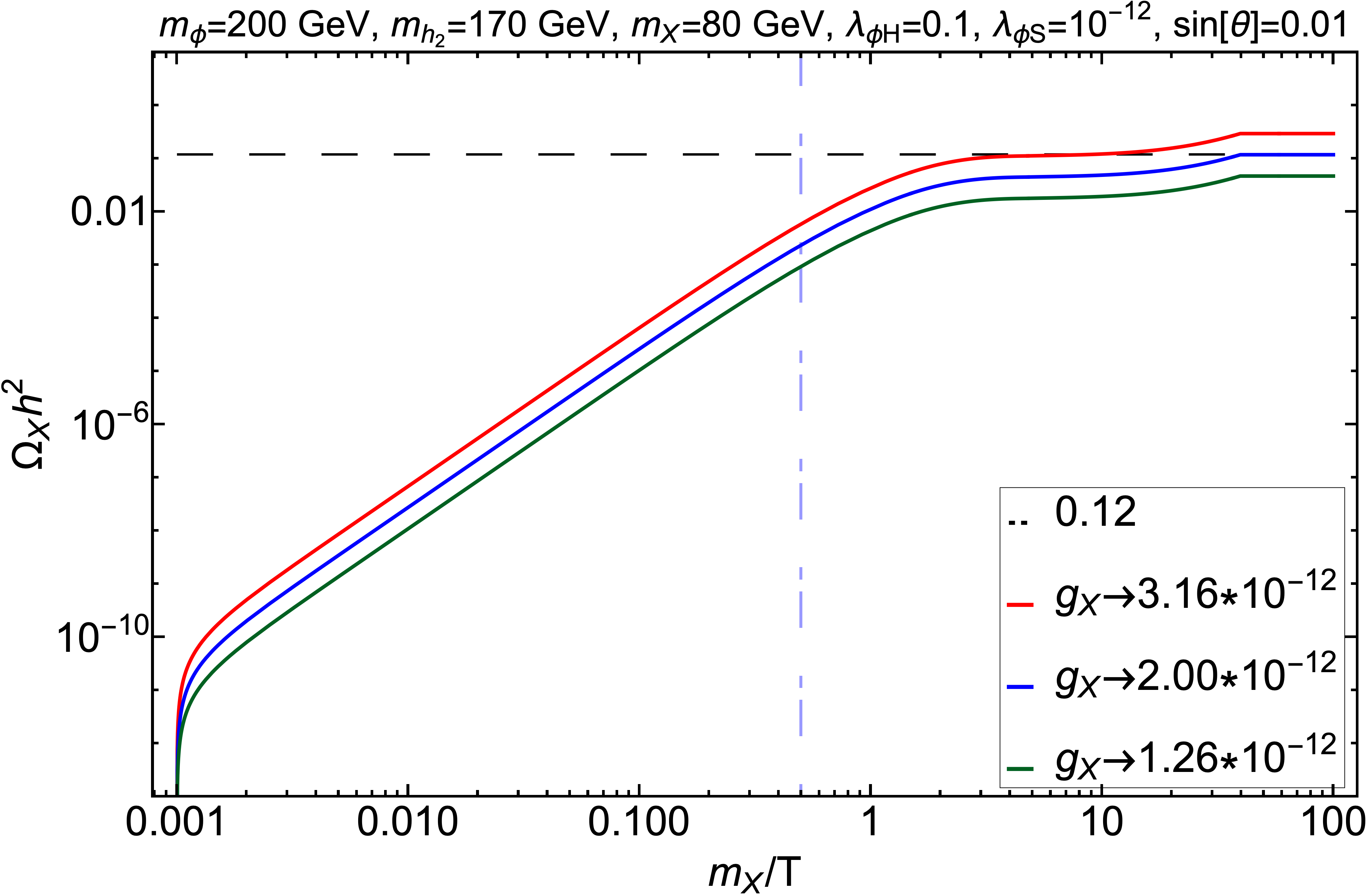
(a)

(b)

Figure 18: Variation of $X$ relic density as a function of $x=m_{X}/T$ to demonstrate freeze-in aEWSB; In left panel (Fig. 19a) we show decay dominant case where freeze-in production aEWSB occurs via $h_{2}\to XX$ for three discrete $g_{X}$ values. In the right panel Fig. LABEL:fimp_aewsb_scattering_m2_l2s, decay is kinematically forbidden and scattering processes dominate freeze-in production. Vertical dot-dashed line indicates EWSB and black dashed line shows the central value of observed relic density. Parameters kept fixed for the plot are mentioned in the figure heading.

(a)

(c)

Figure 19: Under abundant ($\Omega_{X}h^{2}\leq\Omega_{T}h^{2}$) parameter space for DM freeze-in aEWSB. Fig. 19a shows a correlation in $g_{X}$ vs. $m_{X}$ plane with direct search constraint restricting the smaller $g_{X}$ values shown by the grey shaded region. In Fig.LABEL:fimp_aewsb_scattering_m2_l2s, the under abundant region in $\lambda_{\phi S}$ vs. $m_{\phi}$ plane is shown, with grey shaded region ruled out by the XENON1T direct search bound. The relic density of FIMP DM is indicated by color code in the figure inset. In Fig.19c, we show the viable parameter space in $\lambda_{\phi S}$ vs. $g_{X}$ plane for the scattering dominated production of FIMP. Direct search limits weaken for smaller $\lambda_{\phi S}$ and larger $g_{X}$. Parameters kept fixed are mentioned in figure headings.

As the dependence of freeze-in relic density on the parameters remain almost the same aEWSB, it is needless to repeat all the features here once again. Nevertheless, in order to demonstrate the viable parameter space complying with aEWSB freeze-in, we show three plots in Fig. 4.7. The top left plot, i.e., Fig. 19a shows a correlation in $m_{X}$ vs. $g_{X}$ plane and corresponds to the decay dominant FIMP production. We find that excepting for very small $g_{X}$ regions constrained by direct search of $\phi$ (with the direct search cross-section being proportional to $v_{s}\sim 1/g_{X}$), the rest of the parameter space shows under relic abundance indicated by color codes as mentioned in the figure inset. This is an important contrast to the bEWSB case, where the parameter space for the decay dominant FIMP production is completely unconstrained (see Figs.8). Also, one can conclude from this plot that after EWSB, large part of parameter space can be saved from DD limits if the FIMP production is decay dominated. The right panel plot, i.e., Fig. LABEL:fimp_aewsb_scattering_m2_l2s shows a correlation in $m_{\phi}-\lambda_{\phi S}$ plane, which corresponds to scattering dominant FIMP production absent $h_{2}\to XX$ decay. Here we see that a large region of the parameter space is ruled out by DD data particularly for larger $\lambda_{\phi S}$. Since the DD cross-section has very strong dependence on both $\lambda_{\phi S}$ and $g_{X}$, in Fig.19c at the bottom panel, we show a correlation in the $\lambda_{\phi S}$ vs. $g_{X}$ plane. Here, FIMP relic density, although increases with $\lambda_{\phi S}$, remains almost constant with the variation of $g_{X}$, as the scattering dominant production cross-section has no explicit dependence on $g_{X}$. On the other hand, the direct detection cross-section, having explicit dependence on $\lambda_{\phi S}$ and $v_{s}\sim 1/g_{X}$, shows weaker bounds for small $\lambda_{\phi S}$ and large $g_{X}$. Parameters kept fixed for the scans, are mentioned in the respective figure headings and ensure all the other constraints.

5.4 Freeze-out of $\phi$

(a)

(c)

Figure 20: Figure 20a shows freeze-out pattern for WIMP ($\phi$) relic density as a function of $m_{\phi}/T$ for some fixed values of $\lambda_{\phi H}$, which also ensures freeze-out aEWSB. The vertical dot-dashed line corresponding to EWSB ($x_{\rm{EW}}$). Fig. LABEL:wimp_aewsb_m2_l2s denotes a correlation plot for the under-abundant $\phi$ in $m_{\phi}-\lambda_{\phi S}$ plane. The constraints from spin independent DD cross-section obtained from XENON1T data are shown in grey shades. The parameters kept fixed for are mentioned in figure heading. The colour shades in light blue, light red and light yellow show the ranges of under abundance as mentioned in figure inset. In Fig. 20c, we show the under abundant $\phi$ in $\lambda_{\phi S}$ vs. $g_{X}$ plane.

$\phi$ freezes out aEWSB through the annihilation channels as shown in Fig. 16. New annihilation channels open up through for e.g : $h\phi\phi$ vertex aEWSB. The trilinear couplings of $\phi$ with Higgs become relevant in the DM phenomenology, in contrast to only quartic DM-Higgs interaction bEWSB for $\phi$ freeze-out. We demonstrate aEWSB freeze-out with three representative plots in Fig. 4.7. Fig. 20a shows the evolution of WIMP abundance ($\Omega_{\phi}h^{2}$) with $m_{\phi}/T$ for three discrete values (mentioned in the figure inset) represented by red, blue and green coloured lines respectively. If we increase $\lambda_{\phi H}$, this enhances the annihilation cross-section and in turn decrease the relic abundance, which we show in the figure. The blue one with $\lambda_{\phi H}=0.08$ satisfies the correct relic. The vertical dot-dashed line ensures that the $\phi$ freeze out occurs aEWSB and the horizontal dashed line represents the central value of the observed DM relic. Also note in Fig. 20a, a small bump appearing in the equilibrium distribution due to the change of WIMP mass at EWSB boundary as given by Eq. 58 in Appendix LABEL:sec:aEWSB-details.

In Fig. LABEL:wimp_aewsb_m2_l2s, we show the (under-) relic and direct search allowed parameter space in $m_{\phi}-\lambda_{\phi S}$ plane. The three shades light yellow, light red and light blue represent different ranges for under-abundance, as mentioned in the legend. The grey shaded region is excluded by present spin independent direct search (XENON1T) bound. With smaller $\lambda_{\phi S}$, relic density expectedly increases. Also, we see the maximum annihilation around the $m_{h_{2}}$ resonance at 100 GeV, as we fixed $m_{h_{2}}$ at 200 GeV for this scan. Owing to the fact that $m_{h_{2}}$ is unknown and loosely constrained, a large amount of relic density allowed parameter space can be brought under the direct search bound if one focuses on the $m_{h_{2}}$ resonance. We also see that a large parameter space opens up whenever the annihilation channel to $h_{2}$ pair opens up with $m_{\phi}>m_{h_{2}}$. To demonstrate the effect of the two relevant couplings $g_{X}$ and $\lambda_{\phi S}$ on WIMP relic density and DD, we show a correlation plot in the bottom panel Fig. 20c. DD limits show the same trend as Fig. 19c, whereas the WIMP annihilation cross-section, also being proportional to $\lambda_{\phi S}\,v_{s}$, shows under abundance for large $\lambda_{\phi S}$ and small $g_{X}$. Importantly we see that for WIMP, under abundant regions face more exclusion from direct search limit while it is the other way round for FIMP, which obviously stems from the reverse dependence on the cross-section to the DM yield for these two cases.

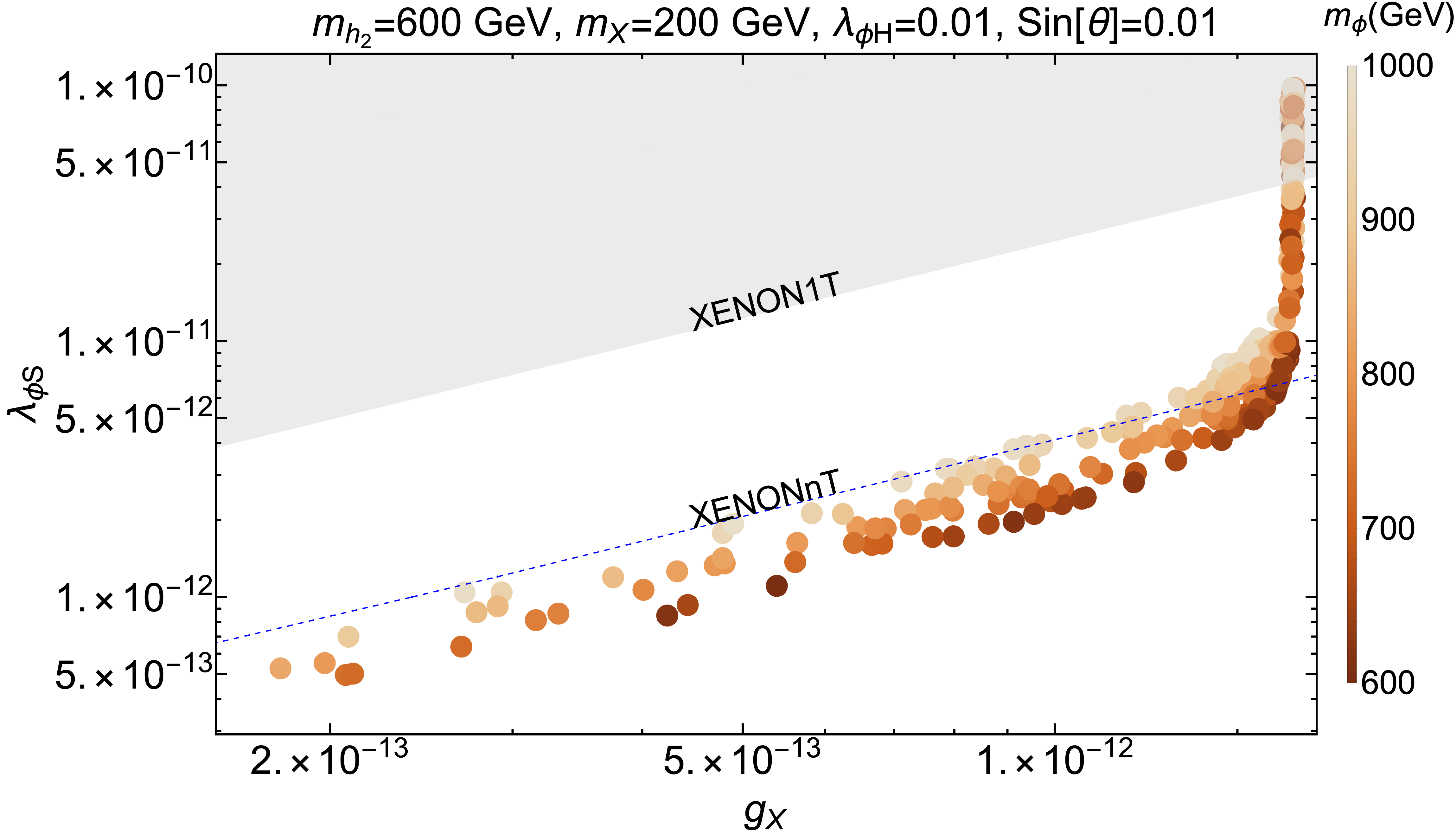
(a)

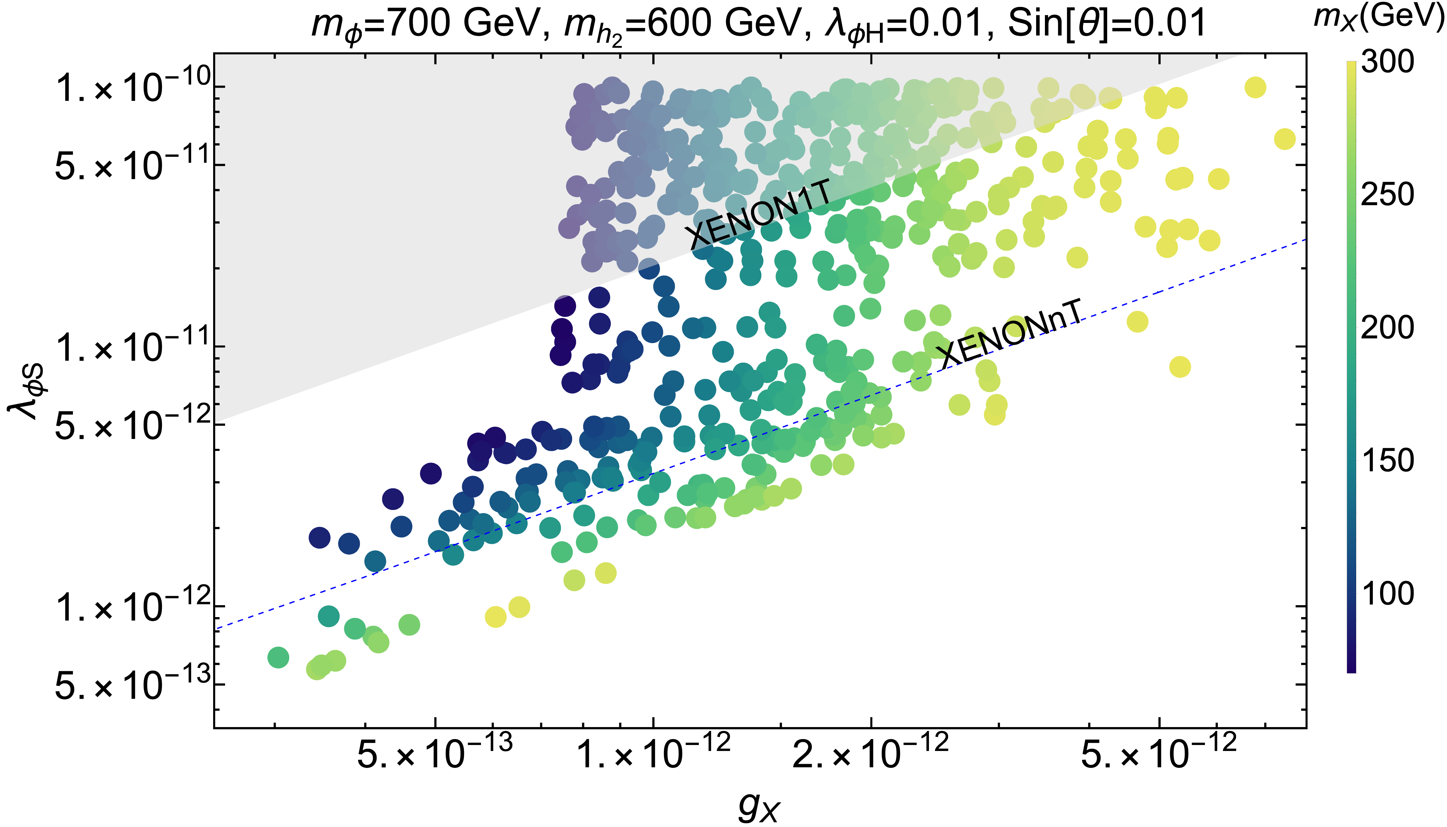
(b)

Figure 21: Scan in $g_{X}-\lambda_{\phi S}$ plane when both WIMP and FIMP components add to observed relic density, $\Omega_{X}h^{2}+\Omega_{\phi}h^{2}=0.1200\pm 0.0012$, simultaneously addressing other constraints when both freeze in and freeze out occur aEWSB in kinematic region $m_{h_{2}}\geq 2m_{X}$. In Fig. 21a, we keep FIMP mass fixed at $m_{X}=200$ GeV and vary WIMP mass $m_{\phi}$ as shown in the SiennaTones colour bar. In Fig. 21b, we keep WIMP mass $m_{\phi}=700$ GeV fixed and vary FIMP mass ($m_{X}$) as shown by the BlueGreenYellow colour bar. Other parameters kept fixed are mentioned in the figure heading. Direct search constraint from XENON1T is shown by grey shaded regions, while the future sensitivity of XENONnT is shown by blue dotted line.

5.5 Putting WIMP and FIMP together

We again discuss a couple of example plots where the WIMP ($\phi$) and FIMP ($X$) add to the total observed DM relic density. In Fig. 21, we show the scan in $g_{X}-\lambda_{\phi S}$ plane where both freeze-in of $X$ and freeze-out of $\phi$ occur aEWSB. In Fig. 21a, we keep FIMP mass ($m_{X}$) fixed, while vary WIMP mass ($m_{\phi}$) as shown by the SiennaTones color bar. In Fig. 21b, we instead keep WIMP mass ($m_{\phi}$) fixed, while vary FIMP mass ($m_{X}$) as shown by the BlueGreenYellow color bar. In both cases, we adhere to a parameter space where FIMP production is decay dominated. Observations are pretty similar to what we got bEWSB.

In Fig. 21a, we again see that with larger $g_{X}$, FIMP relic enhances, which in turn requires $\lambda_{\phi S}$ to enhance as well, so that $\Omega_{\phi}$ decreases (the inclined region). Now, $g_{X}$ can maximally enhance to $\sim 2\times 10^{-12}$, when FIMP relic completely dominates over WIMP, with a sharp rise in $\lambda_{\phi S}$ to bring WIMP relic to very small value. We also see that keeping the $g_{X}$ fixed (so that FIMP relic remains almost unchanged), if we enhance $\lambda_{\phi S}$, WIMP relic decreases unless we adjust $m_{\phi}$ to larger values to keep the total relic within experimental observed value. In Fig. 21b, larger $\lambda_{\phi S}$ diminishes $\Omega_{\phi}$, which is adjusted by larger FIMP contribution, by having smaller $m_{X}$ for a fixed $g_{X}$. Further, when $g_{X}$ is enhanced, FIMP contribution becomes larger, then WIMP contribution is adjusted to smaller values by larger $\lambda_{\phi S}$. Importantly, present direct search bound from XENON1T (on spin independent cross-section) plays an important role here, shown by grey shaded region, which discards part of large $\lambda_{\phi S}$ region. Future projected direct search sensitivity of XENONnT experiment is also shown by the blue dashed line, which will probe a large part of the allowed parameter space.

As can be easily seen, that the phenomenology aEWSB is richer and as the masses ($m_{\phi},m_{s},m_{X}$) turn out to be much smaller. Such regions are prone to both direct search and collider experiments for the WIMP, which interestingly correlates to the FIMP under abundance as some of the parameters are common. We leave the exercise, where collider signal and direct search sensitivity of WIMP-FIMP model will be discussed, for a separate work. We finally tabulate some characteristic benchmark points for this scenario in table LABEL:tab:benchmark_aewsb, where the total relic obtained from $X$ and $\phi$ adds to the observed one abiding by all the other constraints. Here also, AP1 and AP4 point out to the cases when $X$ dominates over $\phi$, AP3, AP6 show when $\phi$ dominates over $X$ and AP2, AP5 depict the case when both DM contribute equally.

(d)

(e)

(f)

Figure 22: Allowed parameter space in $m_{H}-m_{s}$ plane constrained by the requirement of obtaining 125.1 GeV SM Higgs after EWSB. $|\sin[\theta]|\lesssim 0.3$ and $0<\lambda_{H}\leq 4\pi$. FIMP mass ($m_{X}$) is varied in TeV scale in Fig. 22d, 22e and 22f.

The scalar potential can be written only in terms of $h_{1},h_{2},\theta$ is given by

$$V(h_{1},h_{2},\phi)\bigg{|}_{\rm aEWSB}= \frac{\mu_{H}^{2}}{2}(v+h_{1}\cos\theta+h_{2}\sin\theta)^{2}+\frac{\lambda_{H}}{4}(v+h_{1}\cos\theta+h_{2}\sin\theta)^{4}+\frac{\mu_{\phi}^{2}}{2}\phi^{2}$$

$$+\frac{\lambda_{\phi}}{4!}\phi^{4}+\frac{\mu_{S}^{2}}{2}(v_{s}-h_{1}\sin\theta+h_{2}\cos\theta)^{2}+\frac{\lambda_{S}}{4}(v_{s}-h_{1}\sin\theta+h_{2}\cos\theta)^{4}$$

$$+\frac{\lambda_{\phi H}}{4}\phi^{2}(v+h_{1}\cos\theta+h_{2}\sin\theta)^{2}+\frac{\lambda_{\phi S}}{4}\phi^{2}(v_{s}-h_{1}\sin\theta+h_{2}\cos\theta)^{2}$$

$$+\frac{\lambda_{HS}}{4}(v+h_{1}\cos\theta+h_{2}\sin\theta)^{2}(v_{s}-h_{1}\sin\theta+h_{2}\cos\theta)^{2}$$ (55)

Using the extremization condition of the potential

$$\left(\frac{\partial V(h_{1},h_{2},\phi)}{\partial h_{1}}\right),\left(\frac{\partial V(h_{1},h_{2},\phi)}{\partial h_{2}}\right)\bigg{|}_{h_{1,2},\phi=0}=0$$ (56)

we obtain the following conditions,

$$\begin{split}v\cos\theta\left(\lambda_{HS}v_{s}^{2}+2\mu_{H}^{2}+2\lambda_{H}v^{2}\right)-v_{s}\sin\theta\left(v^{2}\lambda_{HS}+2\lambda_{S}v_{s}^{2}+2\mu_{S}^{2}\right)=0\\ v\sin\theta\left(\lambda_{HS}v_{s}^{2}+2\mu_{H}^{2}+2\lambda_{H}v^{2}\right)+v_{s}\cos\theta(v^{2}\lambda_{HS}+2\lambda_{S}v_{s}^{2}+2\mu_{S}^{2})=0\end{split}$$ (57)

$$\begin{split}\frac{\partial^{2}V_{\rm scalar}}{\partial h_{1}^{2}}\bigg{|}_{h_{1,2}=\phi=0}=&m^{2}_{h_{1}}=(3v^{2}\lambda_{H}+\frac{1}{2}v_{s}^{2}\lambda_{HS}+\mu_{H}^{2})\cos^{2}\theta-vv_{s}\lambda_{HS}\sin 2\theta\\ &\qquad+(3v_{s}^{2}\lambda_{S}+\frac{1}{2}v^{2}\lambda_{HS}+\mu_{S}^{2})\sin^{2}\theta\\ \frac{\partial^{2}V_{\rm scalar}}{\partial{\phi}^{2}}\bigg{|}_{h_{1,2}=\phi=0}=&\mathfrak{m}^{2}_{\phi}=\frac{1}{2}\left(2\mu_{\phi}^{2}+\lambda_{\phi S}v_{s}^{2}+v^{2}\lambda_{\phi H}\right)\\ \frac{\partial^{2}V_{\rm scalar}}{\partial h_{2}^{2}}\bigg{|}_{h_{1,2}=\phi=0}=&m_{h_{2}}^{2}=(3v^{2}\lambda_{H}+\frac{1}{2}v_{s}^{2}\lambda_{HS}+\mu_{H}^{2})\sin^{2}\theta+vv_{s}\lambda_{HS}\sin 2\theta\\ &\qquad+(3v_{s}^{2}\lambda_{S}+\frac{1}{2}v^{2}\lambda_{HS}+\mu_{S}^{2})\cos^{2}\theta\end{split}$$ (58)

After mixing, off diagonal mass terms of physical fields $h_{1}$ and $h_{2}$ are absent; then $\partial^{2}V_{\rm scalar}/\partial h_{1}\partial h_{2}=0$ gives us,

$$\cos 2\theta~{}vv_{s}\lambda_{HS}+\frac{1}{2}\sin 2\theta\left[3(v^{2}\lambda_{H}-v_{s}^{2}\lambda_{S})+\frac{1}{2}\lambda_{HS}(v_{s}^{2}-v^{2})-(\mu_{S}^{2}-\mu_{H}^{2})\right]= 0$$ (59)

Finally, the expressions of mixing angle $(\theta)$ and internal parameters $(\mu_{H},\mu_{\phi},\mu_{S},\lambda_{H},\lambda_{S},\lambda_{HS})$ in terms of the external parameters are given by:

$$\begin{split}\mu_{H}^{2}&=-(\lambda_{H}v^{2}+\frac{1}{2}\lambda_{HS}v^{2}_{s}),\\ \mu_{\phi}^{2}&=\mathfrak{m}^{2}_{\phi}-\frac{1}{2}\lambda_{\phi S}v_{s}^{2}-\frac{1}{2}\lambda_{\phi H}v^{2},\\ \mu_{S}^{2}&=-(\lambda_{S}v^{2}_{s}+\frac{1}{2}\lambda_{HS}v^{2}),\\ v_{s}&=\frac{m_{X}}{g_{X}},\\ \lambda_{H}&=\frac{1}{2v^{2}}\left(m^{2}_{h_{1}}\cos^{2}\theta+m^{2}_{h_{2}}\sin^{2}\theta\right),\\ \lambda_{S}&=\frac{1}{2v_{s}^{2}}\left(m^{2}_{h_{2}}\cos^{2}\theta+m^{2}_{h_{1}}\sin^{2}\theta\right),\\ \lambda_{HS}&=\frac{\sin 2\theta}{2v_{s}v}\left(m^{2}_{h_{2}}-m^{2}_{h_{1}}\right).\end{split}$$ (60)

Appendix C Invisible decay width of Higgs

In Higgs portal scenarios, where DM couples to SM Higgs, Higgs boson can always decay to a pair of DM particles when kinematically accessible, contributing to invisible Higgs decay width. In our model, the possible invisible decay channels of Higgs include $h_{1}\to\phi\phi,h_{1}\to XX,h_{1}\to h_{2}h_{2}$ with decay widths given by:

$$\begin{split}&\Gamma_{h_{1}\to\phi\phi}=\frac{(\lambda_{\phi S}m_{X}\sin\theta-\lambda_{\phi H}g_{X}v\cos\theta)^{2}}{32\pi g_{X}^{2}m_{h_{1}}^{2}}(m_{h_{1}}^{2}-4\mathfrak{m}_{\phi}^{2})^{1/2}\Theta(m_{h_{1}}-2\mathfrak{m}_{\phi})\\ &\Gamma_{h_{1}\to XX}=\frac{g_{X}^{2}\sin^{2}\theta}{32\pi m_{h_{1}}^{2}m_{X}^{2}}(m_{h_{1}}^{2}-4m_{X}^{2})^{1/2}(m_{h_{1}}^{4}-4m_{h_{1}}^{2}m_{X}^{2}+12m_{X}^{4})\Theta(m_{h_{1}}-2m_{X})\\ &\Gamma_{h_{1}\to h_{2}h_{2}}=\frac{(m_{X}\sin\theta-vg_{X}\cos\theta)^{2}}{32\pi v^{2}m_{h_{1}}^{2}m_{X}^{2}}\sin^{2}\theta\cos^{2}\theta(m_{h_{1}}^{2}+2m_{h_{2}}^{2})^{2}(m_{h_{1}}^{2}-4m_{h_{2}}^{2})^{1/2}\Theta(m_{h_{1}}-2m_{h_{2}})\end{split}$$ (61)

The expression for the Higgs invisible decay branching ratio is,

$$\Gamma_{h_{1}\to\rm{inv}}=\frac{\Gamma_{h_{1}\to{\phi\phi}}+\Gamma_{h_{1}\to{XX}}+\Gamma_{h_{1}\to{h_{2}h_{2}}}}{\Gamma_{h_{1}}^{\rm{SM}}+\Gamma_{h_{1}\to{\phi\phi}}+\Gamma_{h_{1}\to{XX}}+\Gamma_{h_{1}\to{h_{2}h_{2}}}}.$$ (62)

Invisible Higgs decay widths and branching ratio is heavily restricted by the observed Higgs data at LHC as mentioned in Eq. 24 and therefore, we do not scan the parameter space that comes within.

Appendix D Direct Search possibilities

In this two component WIMP-FIMP DM model, FIMP $X$ coupling to SM Higgs ($H$) (via $s$) $\lambda_{HS}$ is very small in order to facilitate non-thermal production. Therefore, FIMP-nucleon cross-section is negligible. In case of WIMP $\phi$, it can talk to SM through the portals $\lambda_{\phi H}$ and $\lambda_{\phi S}$, given the mixing between $s-h$ present after EWSB, where the physical states become $h_{1}$ and $h_{2}$, out of which $h_{1}$ is assumed as SM Higgs, and $h_{2}$ is dominantly a singlet as explained in Appendix LABEL:sec:aEWSB-details. The Feynman graph for direct search cross-section is shown in Fig. 23. The relative dominance of the mediators $h_{1},h_{2}$ in the DM-nucleon scattering cross-section depends on the mass of new scalar $h_{2}$, which can be either heavy or light.

Figure 23: Feynman diagrams for the direct detection of wimp DM $\phi$.

The spin-independent scattering cross section of $\phi$-Nucleon, mediated by both the physical scalars after mixing, is given by,

$$\sigma^{\rm{SI}}_{n_{\phi}}=\frac{\Omega_{\phi}}{\Omega_{\phi}+\Omega_{X}}\frac{f_{N}^{2}\mu_{n}^{2}m_{n}^{2}}{4\pi v^{2}\mathfrak{m}^{2}_{\phi}}\left(\cos\theta\frac{\lambda_{h_{1}\phi\phi}}{m_{h_{1}}^{2}}+\sin\theta\frac{\lambda_{h_{2}\phi\phi}}{m_{h_{2}}^{2}}\right)^{2}\,,$$ (63)

where $f_{N}=0.308\pm 0.018$ Hoferichter:2017olk represents the form factor of nucleon and $\mu_{n}=\frac{m_{n}\mathfrak{m}_{\phi}}{m_{n}+\mathfrak{m}_{\phi}}$ stands for the reduced mass and $n$ stands for nucleon. Also note that the maximum direct search cross-section for $\phi$ is folded by the fraction of relic density that $\phi$ possess in the total DM relic density in a two component framework given by $\frac{\Omega_{\phi}}{\Omega_{\phi}+\Omega_{X}}$. The expressions of $\lambda_{h_{1}\phi\phi}$ and $\lambda_{h_{2}\phi\phi}$ in terms of our model parameters are given by

$$\lambda_{h_{1}\phi\phi} = -v\cos\theta\lambda_{\phi H}+\frac{m_{X}}{g_{X}}\sin\theta\lambda_{\phi S}\,,$$

$$\lambda_{h_{2}\phi\phi} = -v\sin\theta\lambda_{\phi H}-\frac{m_{X}}{g_{X}}\cos\theta\lambda_{\phi S}.$$ (64)

In our analysis, the $h_{2}$ mediation in the direct detection cross-section is suppressed by small mixing angle. Also, there will be some propagator suppression due to $h_{2}$ which is assumed heavier than the SM Higgs. It is to be noted that if $\sin\theta\sim 0$, ie, mixing is absent, Eq. 63 boils down to the typical scalar singlet direct detection cross-section, mediated by SM Higgs. The constraint on the mixing is propagated to constraining $\lambda_{HS}$, as per Eq. 60, and importantly affects both WIMP and FIMP under abundance. The SI direct search limit from XENON1T is mentioned in 4.2.

We further note that even if freeze-out occurs before EWSB, one can have direct search possibility as described above. Even the FIMP under abundant region gets constrained by direct search bound due to the presence of $\lambda_{\phi S}$ in both the cases. Only when $s$ decay completes before EWSB, it does not mix with $h$ aEWSB and then FIMP has absolutely no connection to SM and no constraints from direct search.

References

- (1) ATLAS collaboration, Observation of a new particle in the search for the Standard Model Higgs boson with the ATLAS detector at the LHC, Phys. Lett. B 716 (2012) 1 [1207.7214].
- (2) CMS collaboration, Observation of a New Boson at a Mass of 125 GeV with the CMS Experiment at the LHC, Phys. Lett. B 716 (2012) 30 [1207.7235].
- (3) G. Isidori, G. Ridolfi and A. Strumia, On the metastability of the standard model vacuum, Nucl. Phys. B 609 (2001) 387 [hep-ph/0104016].
- (4) T. Markkanen, A. Rajantie and S. Stopyra, Cosmological Aspects of Higgs Vacuum Metastability, Front. Astron. Space Sci. 5 (2018) 40 [1809.06923].
- (5) J. Khoury and T. Steingasser, Gauge hierarchy from electroweak vacuum metastability, 2108.09315.
- (6) T.P. Cheng and L.-F. Li, Neutrino Masses, Mixings and Oscillations in SU(2) x U(1) Models of Electroweak Interactions, Phys. Rev. D 22 (1980) 2860.
- (7) S.M. Bilenky and S.T. Petcov, Massive neutrinos and neutrino oscillations, Rev. Mod. Phys. 59 (1987) 671.
- (8) J. Schechter and J.W.F. Valle, Neutrino Masses in SU(2) x U(1) Theories, Phys. Rev. D 22 (1980) 2227.
- (9) M.E. Shaposhnikov, Baryon Asymmetry of the Universe in Standard Electroweak Theory, Nucl. Phys. B 287 (1987) 757.
- (10) D.E. Morrissey and M.J. Ramsey-Musolf, Electroweak baryogenesis, New J. Phys. 14 (2012) 125003 [1206.2942].
- (11) F. Zwicky, Die Rotverschiebung von extragalaktischen Nebeln, Helv. Phys. Acta 6 (1933) 110.
- (12) F. Zwicky, On the Masses of Nebulae and of Clusters of Nebulae, Astrophys. J. 86 (1937) 217.
- (13) Y. Sofue and V. Rubin, Rotation curves of spiral galaxies, Ann. Rev. Astron. Astrophys. 39 (2001) 137 [astro-ph/0010594].
- (14) J.S. Bullock and M. Boylan-Kolchin, Small-Scale Challenges to the CDM Paradigm, Ann. Rev. Astron. Astrophys. 55 (2017) 343 [1707.04256].
- (15) WMAP collaboration, Nine-Year Wilkinson Microwave Anisotropy Probe (WMAP) Observations: Cosmological Parameter Results, Astrophys. J. Suppl. 208 (2013) 19 [1212.5226].
- (16) Planck collaboration, Planck 2018 results. VI. Cosmological parameters, Astron. Astrophys. 641 (2020) A6 [1807.06209].
- (17) P. Gondolo and G. Gelmini, Cosmic abundances of stable particles: Improved analysis, Nucl. Phys. B 360 (1991) 145.
- (18) E.W. Kolb and M.S. Turner, The Early Universe, vol. 69 (1990), 10.1201/9780429492860.
- (19) G. Bertone, D. Hooper and J. Silk, Particle dark matter: Evidence, candidates and constraints, Phys. Rept. 405 (2005) 279 [hep-ph/0404175].
- (20) J.L. Feng, Dark Matter Candidates from Particle Physics and Methods of Detection, Ann. Rev. Astron. Astrophys. 48 (2010) 495 [1003.0904].
- (21) L. Bergstrom, Dark Matter Evidence, Particle Physics Candidates and Detection Methods, Annalen Phys. 524 (2012) 479 [1205.4882].
- (22) L.J. Hall, K. Jedamzik, J. March-Russell and S.M. West, Freeze-In Production of FIMP Dark Matter, JHEP 03 (2010) 080 [0911.1120].
- (23) F. Elahi, C. Kolda and J. Unwin, UltraViolet Freeze-in, JHEP 03 (2015) 048 [1410.6157].
- (24) S. Heeba, F. Kahlhoefer and P. Stöcker, Freeze-in production of decaying dark matter in five steps, JCAP 11 (2018) 048 [1809.04849].
- (25) A. Biswas, S. Ganguly and S. Roy, Fermionic dark matter via UV and IR freeze-in and its possible X-ray signature, JCAP 03 (2020) 043 [1907.07973].
- (26) N. Bernal, M. Heikinheimo, T. Tenkanen, K. Tuominen and V. Vaskonen, The Dawn of FIMP Dark Matter: A Review of Models and Constraints, Int. J. Mod. Phys. A 32 (2017) 1730023 [1706.07442].
- (27) XENON collaboration, Dark Matter Search Results from a One Ton-Year Exposure of XENON1T, Phys. Rev. Lett. 121 (2018) 111302 [1805.12562].
- (28) XENON collaboration, Projected WIMP sensitivity of the XENONnT dark matter experiment, JCAP 11 (2020) 031 [2007.08796].
- (29) PandaX-II collaboration, Results of dark matter search using the full PandaX-II exposure, Chin. Phys. C 44 (2020) 125001 [2007.15469].
- (30) LUX-ZEPLIN collaboration, Projected WIMP sensitivity of the LUX-ZEPLIN dark matter experiment, Phys. Rev. D 101 (2020) 052002 [1802.06039].
- (31) P. Nath et al., The Hunt for New Physics at the Large Hadron Collider, Nucl. Phys. B Proc. Suppl. 200-202 (2010) 185 [1001.2693].
- (32) F. Kahlhoefer, Review of LHC Dark Matter Searches, Int. J. Mod. Phys. A 32 (2017) 1730006 [1702.02430].
- (33) L. Roszkowski, E.M. Sessolo and S. Trojanowski, WIMP dark matter candidates and searches—current status and future prospects, Rept. Prog. Phys. 81 (2018) 066201 [1707.06277].
- (34) G. Belanger et al., LHC-friendly minimal freeze-in models, JHEP 02 (2019) 186 [1811.05478].
- (35) S. Chakraborti, V. Martin and P. Poulose, Freeze-in and freeze-out of dark matter with charged long-lived partners, JCAP 03 (2020) 057 [1904.09945].
- (36) A. Aboubrahim and P. Nath, Detecting hidden sector dark matter at HL-LHC and HE-LHC via long-lived stau decays, Phys. Rev. D99 (2019) 055037 [1902.05538].
- (37) A. Ghosh, T. Mondal and B. Mukhopadhyaya, Heavy stable charged tracks as signatures of non-thermal dark matter at the lhc: a study in some non-supersymmetric scenarios, Journal of High Energy Physics 2017 (2017) 136.
- (38) Q.-H. Cao, E. Ma, J. Wudka and C.P. Yuan, Multipartite dark matter, 0711.3881.
- (39) K.M. Zurek, Multi-Component Dark Matter, Phys. Rev. D 79 (2009) 115002 [0811.4429].
- (40) S. Profumo, K. Sigurdson and L. Ubaldi, Can we discover multi-component WIMP dark matter?, JCAP 12 (2009) 016 [0907.4374].
- (41) S. Bhattacharya, A. Drozd, B. Grzadkowski and J. Wudka, Two-Component Dark Matter, JHEP 10 (2013) 158 [1309.2986].
- (42) A. Biswas, D. Majumdar, A. Sil and P. Bhattacharjee, Two Component Dark Matter : A Possible Explanation of 130 GeV Ray Line from the Galactic Centre, JCAP 1312 (2013) 049 [1301.3668].
- (43) L. Bian, R. Ding and B. Zhu, Two Component Higgs-Portal Dark Matter, Phys. Lett. B 728 (2014) 105 [1308.3851].
- (44) S. Bhattacharya, P. Poulose and P. Ghosh, Multipartite Interacting Scalar Dark Matter in the light of updated LUX data, JCAP 04 (2017) 043 [1607.08461].
- (45) A. DiFranzo and G. Mohlabeng, Multi-component Dark Matter through a Radiative Higgs Portal, JHEP 01 (2017) 080 [1610.07606].
- (46) A. Ahmed, M. Duch, B. Grzadkowski and M. Iglicki, Multi-Component Dark Matter: the vector and fermion case, Eur. Phys. J. C 78 (2018) 905 [1710.01853].
- (47) S. Bhattacharya, P. Ghosh, T.N. Maity and T.S. Ray, Mitigating Direct Detection Bounds in Non-minimal Higgs Portal Scalar Dark Matter Models, JHEP 10 (2017) 088 [1706.04699].
- (48) B. Barman, S. Bhattacharya and M. Zakeri, Multipartite Dark Matter in extension of Standard Model and signatures at the LHC, JCAP 09 (2018) 023 [1806.01129].
- (49) S. Chakraborti and P. Poulose, Interplay of Scalar and Fermionic Components in a Multi-component Dark Matter Scenario, Eur. Phys. J. C 79 (2019) 420 [1808.01979].
- (50) S. Chakraborti, A. Dutta Banik and R. Islam, Probing Multicomponent Extension of Inert Doublet Model with a Vector Dark Matter, Eur. Phys. J. C 79 (2019) 662 [1810.05595].
- (51) S. Bhattacharya, P. Ghosh and N. Sahu, Multipartite Dark Matter with Scalars, Fermions and signatures at LHC, JHEP 02 (2019) 059 [1809.07474].
- (52) F. Elahi and S. Khatibi, Multi-Component Dark Matter in a Non-Abelian Dark Sector, Phys. Rev. D 100 (2019) 015019 [1902.04384].
- (53) S. Bhattacharya, P. Ghosh, A.K. Saha and A. Sil, Two component dark matter with inert Higgs doublet: neutrino mass, high scale validity and collider searches, JHEP 03 (2020) 090 [1905.12583].
- (54) A. Biswas, D. Borah and D. Nanda, Type III seesaw for neutrino masses in model with multi-component dark matter, JHEP 12 (2019) 109 [1908.04308].
- (55) S. Bhattacharya, N. Chakrabarty, R. Roshan and A. Sil, Multicomponent dark matter in extended : neutrino mass and high scale validity, JCAP 04 (2020) 013 [1910.00612].
- (56) A. Betancur, G. Palacio and A. Rivera, Inert doublet as multicomponent dark matter, Nucl. Phys. B 962 (2021) 115276 [2002.02036].
- (57) C.H. Nam, D. Van Loi, L.X. Thuy and P. Van Dong, Multicomponent dark matter in noncommutative gauge theory, JHEP 12 (2020) 029 [2006.00845].
- (58) G. Belanger, A. Mjallal and A. Pukhov, Two dark matter candidates: the case of inert doublet and singlet scalars, 2108.08061.
- (59) A. Dutta Banik, M. Pandey, D. Majumdar and A. Biswas, Two component WIMP–FImP dark matter model with singlet fermion, scalar and pseudo scalar, Eur. Phys. J. C 77 (2017) 657 [1612.08621].
- (60) D. Borah, A. Dasgupta and S.K. Kang, Two-component dark matter with cogenesis of the baryon asymmetry of the Universe, Phys. Rev. D 100 (2019) 103502 [1903.10516].
- (61) S. Peyman Zakeri, S. Mohammad Moosavi Nejad, M. Zakeri and S. Yaser Ayazi, A Minimal Model For Two-Component FIMP Dark Matter: A Basic Search, Chin. Phys. C 42 (2018) 073101 [1801.09115].
- (62) M. Pandey, D. Majumdar and K.P. Modak, Two Component Feebly Interacting Massive Particle (FIMP) Dark Matter, JCAP 06 (2018) 023 [1709.05955].
- (63) M. Duch, B. Grzadkowski and D. Huang, Strongly self-interacting vector dark matter via freeze-in, JHEP 01 (2018) 020 [1710.00320].
- (64) B. Barman, S. Bhattacharya and B. Grzadkowski, Feebly coupled vector boson dark matter in effective theory, JHEP 12 (2020) 162 [2009.07438].
- (65) C. Delaunay, T. Ma and Y. Soreq, Stealth decaying spin-1 dark matter, JHEP 02 (2021) 010 [2009.03060].
- (66) G. Choi, T.T. Yanagida and N. Yokozaki, Feebly interacting gauge boson warm dark matter and XENON1T anomaly, Phys. Lett. B 810 (2020) 135836 [2007.04278].
- (67) B. Barman and A. Ghoshal, Scale Invariant FIMP Miracle, 2109.03259.
- (68) J. McDonald, Gauge singlet scalars as cold dark matter, Phys. Rev. D 50 (1994) 3637 [hep-ph/0702143].
- (69) W.-L. Guo and Y.-L. Wu, The Real singlet scalar dark matter model, JHEP 10 (2010) 083 [1006.2518].
- (70) J.M. Cline, K. Kainulainen, P. Scott and C. Weniger, Update on scalar singlet dark matter, Phys. Rev. D 88 (2013) 055025 [1306.4710].
- (71) T.G. Steele, Z.-W. Wang, D. Contreras and R.B. Mann, Viable dark matter via radiative symmetry breaking in a scalar singlet Higgs portal extension of the standard model, Phys. Rev. Lett. 112 (2014) 171602 [1310.1960].
- (72) V. Silveira and A. Zee, SCALAR PHANTOMS, Phys. Lett. 161B (1985) 136.
- (73) C.P. Burgess, M. Pospelov and T. ter Veldhuis, The Minimal model of nonbaryonic dark matter: A Singlet scalar, Nucl. Phys. B619 (2001) 709 [hep-ph/0011335].
- (74) T. Hambye, Hidden vector dark matter, JHEP 01 (2009) 028 [0811.0172].
- (75) T. Hambye and M.H.G. Tytgat, Confined hidden vector dark matter, Phys. Lett. B 683 (2010) 39 [0907.1007].
- (76) S. Bhattacharya, J.L. Diaz-Cruz, E. Ma and D. Wegman, Dark Vector-Gauge-Boson Model, Phys. Rev. D 85 (2012) 055008 [1107.2093].
- (77) Y. Farzan and A.R. Akbarieh, VDM: A model for Vector Dark Matter, JCAP 10 (2012) 026 [1207.4272].
- (78) Z. Hu, C. Cai, Y.-L. Tang, Z.-H. Yu and H.-H. Zhang, Vector dark matter from split SU(2) gauge bosons, JHEP 07 (2021) 089 [2103.00220].
- (79) S. Baek, P. Ko, W.-I. Park and E. Senaha, Higgs Portal Vector Dark Matter : Revisited, JHEP 05 (2013) 036 [1212.2131].
- (80) P. Ko, W.-I. Park and Y. Tang, Higgs portal vector dark matter for scale -ray excess from galactic center, JCAP 09 (2014) 013 [1404.5257].
- (81) M. Duch, B. Grzadkowski and M. McGarrie, A stable Higgs portal with vector dark matter, JHEP 09 (2015) 162 [1506.08805].
- (82) M. Duch and B. Grzadkowski, Resonance enhancement of dark matter interactions: the case for early kinetic decoupling and velocity dependent resonance width, JHEP 09 (2017) 159 [1705.10777].
- (83) S. Yaser Ayazi and A. Mohamadnejad, Conformal vector dark matter and strongly first-order electroweak phase transition, JHEP 03 (2019) 181 [1901.04168].
- (84) G. Choi, T.T. Yanagida and N. Yokozaki, Dark photon dark matter in the minimal model, JHEP 01 (2021) 057 [2008.12180].
- (85) O. Lebedev, H.M. Lee and Y. Mambrini, Vector Higgs-portal dark matter and the invisible Higgs, Phys. Lett. B 707 (2012) 570 [1111.4482].
- (86) H. Davoudiasl and I.M. Lewis, Dark Matter from Hidden Forces, Phys. Rev. D 89 (2014) 055026 [1309.6640].
- (87) S. Bhattacharya and J. Wudka, Effective Theories with Dark Matter Applications, 2104.01788.
- (88) A.L. Fitzpatrick, W. Haxton, E. Katz, N. Lubbers and Y. Xu, The Effective Field Theory of Dark Matter Direct Detection, JCAP 02 (2013) 004 [1203.3542].
- (89) F. Fortuna, P. Roig and J. Wudka, Effective field theory analysis of dark matter-standard model interactions with spin one mediators, JHEP 02 (2021) 223 [2008.10609].
- (90) S. Matsumoto, S. Mukhopadhyay and Y.-L.S. Tsai, Singlet Majorana fermion dark matter: a comprehensive analysis in effective field theory, JHEP 10 (2014) 155 [1407.1859].
- (91) N.F. Bell, Y. Cai, J.B. Dent, R.K. Leane and T.J. Weiler, Dark matter at the LHC: Effective field theories and gauge invariance, Phys. Rev. D 92 (2015) 053008 [1503.07874].
- (92) A. De Simone and T. Jacques, Simplified models vs. effective field theory approaches in dark matter searches, Eur. Phys. J. C 76 (2016) 367 [1603.08002].
- (93) Q.-H. Cao, C.-R. Chen, C.S. Li and H. Zhang, Effective Dark Matter Model: Relic density, CDMS II, Fermi LAT and LHC, JHEP 08 (2011) 018 [0912.4511].
- (94) K. Cheung, P.-Y. Tseng, Y.-L.S. Tsai and T.-C. Yuan, Global Constraints on Effective Dark Matter Interactions: Relic Density, Direct Detection, Indirect Detection, and Collider, JCAP 05 (2012) 001 [1201.3402].
- (95) G. Busoni, A. De Simone, E. Morgante and A. Riotto, On the Validity of the Effective Field Theory for Dark Matter Searches at the LHC, Phys. Lett. B 728 (2014) 412 [1307.2253].
- (96) M. Duch, B. Grzadkowski and J. Wudka, Classification of effective operators for interactions between the Standard Model and dark matter, JHEP 05 (2015) 116 [1412.0520].
- (97) M. Carena, A. Megevand, M. Quiros and C.E.M. Wagner, Electroweak baryogenesis and new TeV fermions, Nucl. Phys. B 716 (2005) 319 [hep-ph/0410352].
- (98) M.J. Baker and L. Mittnacht, Variations on the Vev Flip-Flop: Instantaneous Freeze-out and Decaying Dark Matter, JHEP 05 (2019) 070 [1811.03101].
- (99) V. De Romeri, D. Karamitros, O. Lebedev and T. Toma, Neutrino dark matter and the Higgs portal: improved freeze-in analysis, JHEP 10 (2020) 137 [2003.12606].
- (100) M. Chianese and S.F. King, The Dark Side of the Littlest Seesaw: freeze-in, the two right-handed neutrino portal and leptogenesis-friendly fimpzillas, JCAP 09 (2018) 027 [1806.10606].
- (101) J. Elias-Miro, J.R. Espinosa, G.F. Giudice, H.M. Lee and A. Strumia, Stabilization of the Electroweak Vacuum by a Scalar Threshold Effect, JHEP 06 (2012) 031 [1203.0237].
- (102) K. Kannike, Vacuum Stability of a General Scalar Potential of a Few Fields, Eur. Phys. J. C 76 (2016) 324 [1603.02680].
- (103) J. Chakrabortty, P. Konar and T. Mondal, Copositive Criteria and Boundedness of the Scalar Potential, Phys. Rev. D 89 (2014) 095008 [1311.5666].
- (104) G. Bhattacharyya and D. Das, Scalar sector of two-Higgs-doublet models: A minireview, Pramana 87 (2016) 40 [1507.06424].
- (105) J. Horejsi and M. Kladiva, Tree-unitarity bounds for THDM Higgs masses revisited, Eur. Phys. J. C 46 (2006) 81 [hep-ph/0510154].
- (106) G. Chalons, D. Lopez-Val, T. Robens and T. Stefaniak, The Higgs singlet extension at LHC Run 2, PoS DIS2016 (2016) 113 [1606.07793].
- (107) V. Barger, P. Langacker, M. McCaskey, M.J. Ramsey-Musolf and G. Shaughnessy, LHC Phenomenology of an Extended Standard Model with a Real Scalar Singlet, Phys. Rev. D 77 (2008) 035005 [0706.4311].
- (108) E. Fuchs, O. Matsedonskyi, I. Savoray and M. Schlaffer, Collider searches for scalar singlets across lifetimes, JHEP 04 (2021) 019 [2008.12773].
- (109) CMS collaboration, Searches for Higgs boson rare and invisible decays at CMS, PoS ICHEP2020 (2021) 070.
- (110) ATLAS collaboration, Combination of searches for invisible Higgs boson decays with the ATLAS experiment, .
- (111) S. Okawa and Y. Omura, Light mass window of lepton portal dark matter, JHEP 02 (2021) 231 [2011.04788].
- (112) B. Barman, S. Bhattacharya and M. Zakeri, Non-Abelian Vector Boson as FIMP Dark Matter, JCAP 02 (2020) 029 [1905.07236].
- (113) J. Buch, P. Ralegankar and V. Rentala, Late decaying 2-component dark matter scenario as an explanation of the AMS-02 positron excess, JCAP 10 (2017) 028 [1609.04821].
- (114) G. Bélanger, F. Boudjema, A. Goudelis, A. Pukhov and B. Zaldivar, micrOMEGAs5.0 : Freeze-in, Comput. Phys. Commun. 231 (2018) 173 [1801.03509].
- (115) J.C. Criado, A. Djouadi, M. Perez-Victoria and J. Santiago, A complete effective field theory for dark matter, JHEP 07 (2021) 081 [2104.14443].
- (116) A. Falkowski, G. Isabella and C.S. Machado, On-shell effective theory for higher-spin dark matter, SciPost Phys. 10 (2021) 101 [2011.05339].
- (117) W.R. Inc., “Mathematica, Version 12.3.1.0.”
- (118) J. Redondo and M. Postma, Massive hidden photons as lukewarm dark matter, JCAP 02 (2009) 005 [0811.0326].
- (119) M.J. Baker, M. Breitbach, J. Kopp and L. Mittnacht, Dynamic Freeze-In: Impact of Thermal Masses and Cosmological Phase Transitions on Dark Matter Production, JHEP 03 (2018) 114 [1712.03962].
- (120) M. Hoferichter, P. Klos, J. Menéndez and A. Schwenk, Improved limits for Higgs-portal dark matter from LHC searches, Phys. Rev. Lett. 119 (2017) 181803 [1708.02245].