Interpretable AI forecasting for numerical relativity waveforms
of quasi-circular, spinning, non-precessing binary black hole mergers

Abstract

We present a deep-learning artificial intelligence model that is capable of learning and forecasting the late-inspiral, merger and ringdown of numerical relativity waveforms that describe quasi-circular, spinning, non-precessing binary black hole mergers. We used the NRHybSur3dq8 surrogate model to produce train, validation and test sets of $\ell=|m|=2$ waveforms that cover the parameter space of binary black hole mergers with mass-ratios $q\leq 8$ and individual spins $|s^{z}_{\{1,\,2\}}|\leq 0.8$. These waveforms cover the time range $t\in[-5000\textrm{M},130\textrm{M}]$, where $t=0M$ marks the merger event, defined as the maximum value of the waveform amplitude. We harnessed the ThetaGPU supercomputer at the Argonne Leadership Computing Facility to train our AI model using a training set of 1.5 million waveforms. We used 16 NVIDIA DGX A100 nodes, each consisting of 8 NVIDIA A100 Tensor Core GPUs and 2 AMD Rome CPUs, to fully train our model within 3.5 hours. Our findings show that artificial intelligence can accurately forecast the dynamical evolution of numerical relativity waveforms in the time range $t\in[-100\textrm{M},130\textrm{M}]$. Sampling a test set of 190,000 waveforms, we find that the average overlap between target and predicted waveforms is $\gtrsim 99\%$ over the entire parameter space under consideration. We also combined scientific visualization and accelerated computing to identify what components of our model take in knowledge from the early and late-time waveform evolution to accurately forecast the latter part of numerical relativity waveforms. This work aims to accelerate the creation of scalable, computationally efficient and interpretable artificial intelligence models for gravitational wave astrophysics.

I Introduction

The combination of artificial intelligence (AI) and innovative computing has led to novel, computationally efficient and scalable methodologies for gravitational wave detection [1, 2, 3, 4, 5, 6, 7, 8, 9, 10, 11, 12, 13, 14, 15, 16, 17], denoising [18, 19, 20], parameter estimation [21, 22, 23, 24, 25, 26], rapid waveform production [27, 28], and early warning systems for multi-messenger sources [29, 30, 31], to mention a few. The convergence of AI, distributed computing and scientific data infrastructure has enabled the creation of production scale, AI-driven frameworks for gravitational wave detection [32, 33, 34]. The fact that these advances have stemmed from prototypes to search for gravitational waves in advanced Laser Interferometer Gravitational Wave Observatory (LIGO) data [2] into production scale AI frameworks that process advanced LIGO data in bulk [29, 30, 31] within just five years, and that these methodologies have been embraced and developed by multiple teams around the world, furnish evidence for the transformational, global impact of AI and innovative computing in gravitational wave astrophysics [35, 36, 37].

AI has also been harnessed to learn and describe multi-scale and multi-physics phenomena, such as the physics of subgrid-scale ideal magnetohydrodynamics turbulence of 2D simulations of the magnetized Kelvin-Helmholtz instability [38]. The creation of AI surrogates is an active area of research that aims to improve the computational efficiency, scalability and accuracy of scientific software utilized in conjunction with high-performance computing (HPC) platforms to study and simulate complex phenomena [39, 40]. It is in the spirit of this work, that researchers have explored the ability of AI to forecast the non-linear behavior of waveforms that describe the physics of quasi-circular, non-spinning, binary black hole mergers [41].

In this study we quantify the ability of AI to learn and describe the highly dynamical, non-linear behaviour of numerical relativity waveforms that describe quasi-circular, spinning, non-precessing binary black hole mergers. To do this, we have implemented a deep-learning AI model that takes as input time-series waveform data that describes the inspiral evolution, and then outputs time-series data that describes the late-inspiral, merger and ringdown of binary black holes that span systems with mass-ratios $1\leq q\leq 8$, and individual spins $s^{z}_{{1,2}}\in[-0.8,0.8]$. To make apparent the size and complexity of this problem, the astute reader may notice that the amount of training data to address this problem in the context of non-spinning, quasi-circular binary black hole mergers is of order $\sim 1.2\times 10^{4}$ [41]. In stark contrast, addressing this problem in the context of quasi-circular, spinning, non-precessing binary black hole mergers requires a training dataset that contains over $\sim 1.5\times 10^{6}$ modeled waveforms to densely sample this high dimensional signal manifold. This amount of data is needed to capture the rich dynamics imprinted in the waveforms that describe these astrophysical systems. The strategy we have followed to tackle this computational grand challenge consists of combining AI and HPC to reduce time-to-insight, and to incorporate a number of methodologies to create our Transformer based AI model, including positional encoding, multi-head self-attention, multi-head cross attention, layer normalization, and residual connections.

Furthermore, we acknowledge the importance of going beyond innovative algorithm design, and the confluence of AI and HPC to address these types of computational challenges. There is a pressing need to understand how AI models abstract knowledge from data and make predictions. Thus, we also showcase the use of scientific visualization and HPC to interpret and understand how various components of our AI model work together to make accurate predictions. Throughout this paper we use geometric units in which $G=c=1$. In this convention, $M$ sets the length scale of the scale invariant black hole simulations, and corresponds to the total mass of the spacetime simulated. For instance, $M=1M_{\odot}=4.93\times 10^{-6}\textrm{ s}$ or $M=1M_{\odot}=1.48\textrm{ km}$. In this article we use $M$ to describe time.

This article is organized as follows. Section II describes the datasets, neural network architecture and optimization methods used to create our AI model. We present and discuss our results in Section III. This section includes a detailed study of the forecasting capabilities of our AI model, as well as interpretability studies. Finally, we summarize our findings and outline future work in Section IV.

II Methods

Here we describe the waveform datasets used for this study, the key components of our AI model, and the approaches followed to train and optimize it.

II.1 Dataset

We consider inspiral-merger-ringdown waveforms that describe quasi-circular, spinning, non-precessing binary black hole mergers. We have produced training, test and validation waveform sets with the surrogate model NRHybSur3dq8 [42]. Since the surrogate NRHybSur3dq8 is trained with 104 numerical relativity waveforms in the parameter range $q\leq 8$ and $|s^{z}_{i}|\leq 0.8$, we restrict our datasets to lie within the same parameter span. Throughout this paper we use a geometric unit system in which $G=c=1$.

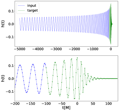
We use $\ell=|m|=2$ waveforms for this study that cover the time span $t\in[-5,000\,\textrm{M},130\,\textrm{M}]$ with the merger (amplitude peak of the signal) occurring at $t=0M$. To accurately capture the dynamics of the waveform we sample it with a time step $\Delta t=2\,\textrm{M}$. We split each waveform into two segments, namely, the input consisting of the early inspiral phase covering the time span $t\in[-5,000\,\textrm{M},-100\,\textrm{M}]$, and the target consisting of late-inspiral, merger and ringdown covering the time span $t\in[-100\,\textrm{M},130\,\textrm{M}]$. We then train an AI model to forecast the target waveform segment when fed with the input waveform segment. An example waveform with the input and target segments is shown in Figure 1.

Figure 1: Left panel Training, validation and test sets for the binary black hole 3-D signal manifold $1\leq q\leq 8$ and $s^{z}_{\{1,2\}}\in[-0.8,0.8]$. 1.5M waveforms are used for the training set, and 190,00 waveforms for the test and validation sets. The sampling shown in this 3-D representation for $q\in[1,1.8)$ is mirrored throughout the parameter space under consideration. Top-right panel Sample waveform for a binary black hole with parameters $\{q,s^{z}_{1},s^{z}_{2}\}=\{6.8,0.718,0.718\}$. Signals span the time window $t\in[-5000M,130M]$ sampled with a time step $\Delta t=2\,\textrm{M}$. Bottom-right panel Input data to our AI model spans the time window $t\leq-100M$, whereas $t\geq-100M$ represents the target time-series output.

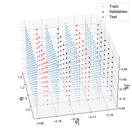
The training set consists of $\sim 1.5$ million waveforms generated by sampling the mass-ratio $q\in[1,8]$ in steps of $\Delta q=0.08$, and the individual spins $s^{z}_{i}\in[-0.8,0.8]$ in steps of $\Delta s^{z}_{i}=0.012$. The validation and test sets consist of $\sim 190,000$ waveforms each, and are generated by alternately sampling the intermediate values, i.e., by sampling $q$ and $s^{z}_{i}$ in steps of $0.16$ and $0.024$ to lie between training set values. We show a small slice of the parameter space to illustrate this sampling in Figure 1.

II.2 Neural network architecture

The neural network we use for numerical relativity waveform forecasting is a slightly modified version of the Transformer model, originally proposed in the context of Natural Language Processing (NLP) [43]. The fundamental operation in the Transformer model is the multi-head scaled dot-product Attention mechanism. Attention can be thought of as a mapping between two sets; each element of the output set is a weighted average of all elements in the input set, where the weights are assigned according to some scoring function. This helps with context aware memorization of long sequences. We briefly discuss the various components of the Transformer model below.

II.2.1 Scaled dot-product attention

Consider a set of n input vectors $\{x_{1},x_{2},x_{3},...,x_{n}\}$ and a set of $t$ output vectors $\{h_{1},h_{2},h_{3},...,h_{t}\}$ in $\mathbb{R}^{d}$. Then according to scaled dot product attention, the outputs are computed as follows:

$$h_{i}=\sum_{j}w_{ij}v_{j}\,,$$ (1)

where,

$$w_{ij} =\texttt{softmax}\left(\frac{q_{i}^{T}k_{j}}{\sqrt{d}}\right)\,,$$ (2)

$$q_{i} =W_{q}x_{i}\,,$$ (3)

$$k_{i} =W_{k}x_{i}\,,$$ (4)

$$v_{i} =W_{v}x_{i}\,,$$ (5)

where $W_{q}$, $W_{k}$ and $W_{v}$ are three learnable weight matrices and each of the three vectors $q_{i}$, $k_{i}$, $v_{i}$ (referred to as queries, keys and values) are linear transformations of the specific input $x_{i}$.

II.2.2 Self and cross attention

Self attention refers to applying the attention mechanism to relate different elements of a single set, i.e., queries, keys and values all correspond to the linear transformations of the same set of vectors $\{x_{i}\}$ as above. However, in cross attention the queries can come from a different set of vectors $\{y_{i}\}$, i.e., $q_{i}=W_{q}y_{i}$.

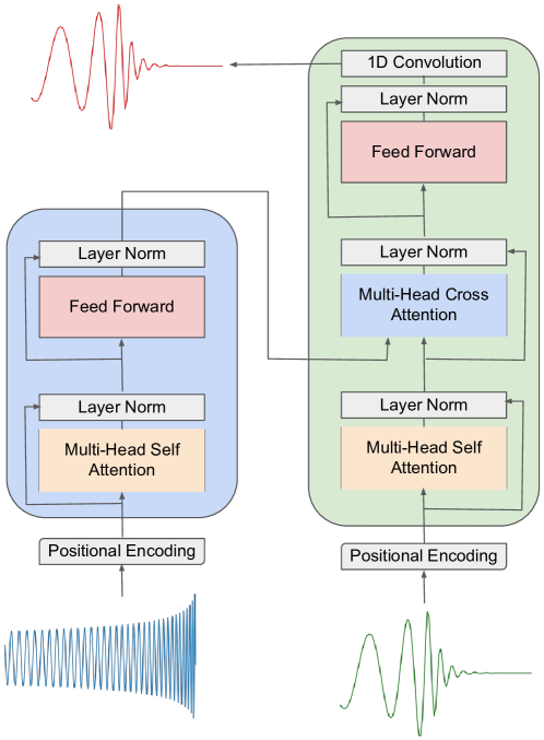
In our case, the set $\{x_{1},x_{2},x_{3},...,x_{n}\}$ corresponds to the input waveform segment and the set $\{y_{1},y_{2},y_{3},...,y_{t}\}$ corresponds to the target waveform segment. These are shown in blue and green respectively in the right panels of Figure 1.

II.2.3 Multi-head Attention

Multi-head attention simply refers to applying the attention operation several times in parallel to independently projected queries, keys and values, i.e., for $n$ heads we would have $n$ sets of the three matrices; $W_{q}^{i}$, $W_{k}^{i}$ and $W_{v}^{i}$, $i\in\{1,2,3,..,n\}$. To do this efficiently, the multi-head attention module first splits the input vector $x_{i}$ into $n$ smaller chunks, and then computes the attention scores over each of the $n$ subspaces in parallel.

II.2.4 Positional encoding

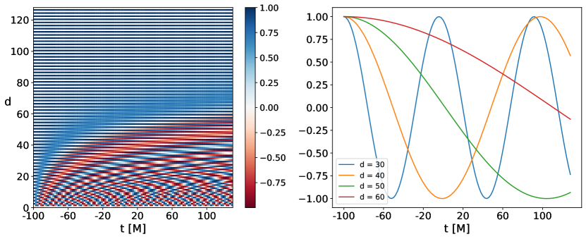
In our case, the inputs and output waveform segments are not sets but ordered time-series sequences. However, we can see from Equation 1 that attention mechanism is permutation equivariant, i.e., it ignores the sequential nature of the input. In order to make the model sensitive to the sequential ordering of the data, we inject information about the absolute positioning of the time-steps in the form of Positional Encoding (PE), i.e., some fixed function $f:\mathbb{N}\to\mathbb{R}^{d}$ to map the positions to real valued vectors. Following the original Transformer paper, we compute the positional encodings as follows:

$$\texttt{PE}(p,2i) =\sin(p/10000^{2i/d})\,,$$ (6)

$$\texttt{PE}(p,2i+1) =\cos(p/10000^{2i/d})\,,$$ (7)

where $p$ is the position and $i$ is the dimension. A sample encoding for $d=128$, used for the actual analysis conducted in this paper, is shown in Figure 2. It is worth mentioning that the dimension $d$ is a hyper-parameter and has to be tuned for optimal performance.

At the fundamental level, the input to our model is $1$ dimensional (a 1D wave). However, we transform this data from rank-1 to rank-2, i.e., from a sequence of real numbers of amplitude values $(h_{1},h_{2},…,h_{n})$ to a sequence of $d+1$ dimensional vectors $(\mathbf{v_{1}},\mathbf{v_{2}},…,\mathbf{v_{n}})$, where each $\mathbf{v_{i}}=[h_{i},\texttt{PE}(i,1),\texttt{PE}(i,2),\texttt{PE}(i,3),...,\texttt{PE}(i,d)]$, and $\texttt{PE}(i,n)$ is given by equations 6 and 7.

We do this because we want the model to be aware of the time-stamp of each amplitude value. One could in principle do this by inputting into the model a tuple $(h_{i},t_{i})$ instead of just the sequence of amplitude values $(h_{i},)$. However, positional encodings in the manner described above have historically worked much better.

Figure 2: Left panel Heatmap of the evaluation of the positional encodings— see Eqs.(6)-(7). These real-valued vectors are computed at each timestamp of the target waveform $t\in[-100\textrm{M},130\textrm{M}]$—shown in the x-axis, for each dimension $d$—shown in the y-axis. Right panel Sample of encodings evaluated at several timestamps and dimensions. The encoding at each dimension $d$ is a sinusoid of a different frequency.

II.2.5 Encoder and decoder modules

The Transformer model consists of an encoder module and a decoder module. The encoder takes in an input sequence $\{x_{1},x_{2},$ $x_{3},...,x_{n}\}$, passes it through a multi-head self-attention layer and a position-wise fully connected feed-forward network, mapping it to an attention based latent vector representation $\{h_{1},h_{2},h_{3},...,h_{n}\}$. This latent representation is then passed to the decoder module, which outputs the desired target sequence $\{y_{1},y_{2},y_{3},...,y_{t}\}$. At each time-step $t=i$ when the decoder is predicting $y_{i}$, it passes the thus-far generated output sequence $\{y_{1},y_{2},y_{3},...,y_{i-1}\}$ through a multi-head self-attention layer and the latent vector representation $\{h_{1},h_{2},h_{3},...,h_{n}\}$ through a multi-head cross attention layer. The two are added together and passed through a position-wise fully connected feed-forward network and a final 1D convolutional layer to generate the next time-step of the output sequence $y_{i}$ in an autoregressive fashion.

Both the encoder and decoder modules also make use of layer normalization and residual connections. We refer the reader for a more in depth discussion of the Transformer model to the original paper [43]. We summarize the architecture for our model in Figure 3.

Figure 3: Model architecture Schematic representation of our AI model. During training we provide two input waveforms, namely, a pre-merger waveform that spans the time range $t\leq-100\textrm{M}$—shown at the bottom left of the diagram; and a time-shift version of the target waveform that spans the time range $t\in[-101\textrm{M},129\textrm{M}]$—shown at the bottom right of the diagram. The output of this AI model, the target waveform that spans the range $t\in[-100\textrm{M},130\textrm{M}]$, is shown at the top left of this diagram. At inference, we provide an input waveform—as indicated in the bottom left of the diagram. The model then outputs time samples up to time $i$, which are then passed as input—as shown in the bottom right panel of the figure—so that the model produces the following time samples up to time $i+1$. The final output is a waveform that covers the range $t\in[-100\textrm{M},130\textrm{M}]$.

II.3 Training and optimization

As mentioned above, we first divide the waveforms into input segments corresponding to $t\in[-5000\,\textrm{M},-100\,\textrm{M}]$, and target segments corresponding to $t\in[-100\,\textrm{M},130\,\textrm{M}]$. We then concatenate both segments with their respective fixed positional encodings. In our experiments, we trained two models; one on only the plus polarization waveforms and another on a dataset composed of equal number of plus and cross polarization waveforms. However, we did not find a significant difference in the performance between these two models, i.e. the model trained on only plus polarizations was just as good at generalizing to the cross polarizations, as the model that was trained on both. Consequently, in this paper we report results for the model that was trained only on the plus polarization, but during inference it is used to predict both plus and cross polarization. During training time we employ the Teacher Forcing methodology, i.e., we pass the input segment through the encoder, and a one step time-shifted version of the target to the decoder. This means that true output is fed to the decoder for the next time step prediction regardless of the predicted value at the current time-step, which helps the model converge faster. A visual exposition of this methodology is presented in Appendix A.

We use mean-squared error (MSE) between the predicted and the target series as the loss function, and use Adam optimizer with $\beta_{1}=0.9,\beta_{2}=0.999,\epsilon=1e-07$ and learning_rate $=0.001$. During training we also monitor the loss on the validation set to prevent over-fitting and to dynamically reduce the learning rate whenever the loss hits a plateau.

We trained our AI model using 16 NVIDIA DGX A100 nodes at the Argonne Leadership Computing Facility. Each node comprises of eight NVIDIA A100 Tensor Core GPUs and two AMD Rome CPUs that provide 320 gigabytes of GPU memory. We used a batch-size of 8 and trained the model for a total of 53 epochs, reaching convergence in 3.5 hours.

III Results

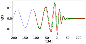
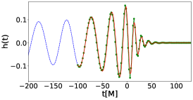
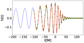
During inference, we only feed the input segment to the model and let it recover the full target sequence autoregressively, i.e., to make the prediction at time-step $t=i$, the decoder module is fed its own prediction from the previous time-step $t=i-1$. Our AI model outputs both the plus and cross polarizations. We show a representative sample of target and predicted waveforms in Figure 4. We have selected these cases to provide a visual representation of the rich dynamics captured by our AI model, encompassing rapid plunges represented by black hole binaries whose components have negative spins (left column); non-spinning binary black holes (mid column); and systems that, on account of having binary components with positive spins and thus more angular momentum, complete more waveform cycles before plunge (right column).

Figure 4: Gallery of results Sample input, target and predicted waveforms for binary black holes with mass-ratios $q=\{1.04,4.24,6.80\}$, from top to bottom; and spins $s^{z}_{1}=s^{z}_{2}=\{-0.7,0.0,0.7\}$, from left to right. Notice the impact of individual spins in the dynamics of the systems, encompassing rapid (left column) and delayed plunges (right column). The model predicts the waveform evolution in the range $-100\textrm{M}\leq t\leq 130\textrm{M}$.

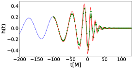
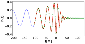
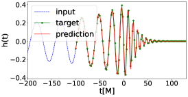
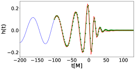
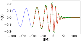
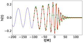
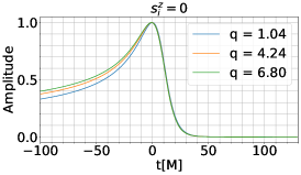
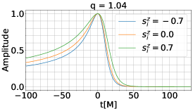
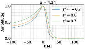
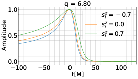
To get a visual representation of the type of dynamics that our AI model needs to capture, we present in Figure 5 the normalized waveform amplitude of the binary black hole systems considered in Figure 4. Key points to extract from these results include:

• Top panel: Quasi-circular, non-spinning, binary black holes display a well known universal behaviour in the vicinity of merger. These physical properties facilitate the training of AI models for these types of systems.

• Bottom panels: We notice the role individual spins play in modulating the waveform amplitude, and driving the systems to merger. These physical properties are one of the most challenging features to capture for waveform modeling experts who aim to accurately describe the late-time evolution of spinning, non-precessing binary black hole mergers. In this study we have demonstrated that AI may accomplish such a task in data-driven manner.

Figure 5: Top panel Near universal behaviour in the dynamical evolution of quasi-circular, non-spinning binary black hole mergers in the vicinity of merger $(t=0\textrm{M})$. Bottom panels Individual spins modulate the waveform amplitude, and drive binary black holes to merger in distinct ways, namely, rapid merger (left panel) and delayed merger (right panel). Notice the distinct features of the normalized amplitude for each system near merger. These subtle differences in waveform dynamics are highly non-trivial to capture by semi-analytical waveform models, though AI can accurately learn and predict these properties in a data-driven fashion.

We have quantified the accuracy of our model’s predictions by computing the overlap, ${\cal{O}}(h_{t},\,h_{p})$, between the target waveform $h_{t}$ and the predicted waveform $h_{p}$

$${\cal{O}}(h_{t},\,h_{p})=\underset{t_{c}\,\phi_{c}}{\mathrm{max}}\left(\hat{h}_{t}|\hat{h}_{p}{[t_{c},\,\phi_{c}]}\right)\,,$$

$$\quad{\rm with}\quad\hat{h}_{t}=h_{t}\,\left(h_{t}|h_{t}\right)^{-1/2}\,,$$ (8)

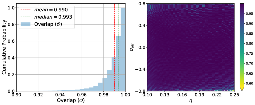
where $\hat{h}_{p}{[t_{c},\,\phi_{c}]}$ indicates that the normalized waveform $\hat{h}_{p}$ has been time- and phase-shifted. Hence, the overlap $\cal{O}$ lies in $[0,1]$, reaching the maximum value of $1$ for a perfect match. To visualize our findings, we first recast the parameter space $(q,s_{1}^{z},s_{2}^{z})$ into symmetric mass ratio $\eta$ and effective spin $\sigma_{\textrm{eff}}$ using the relations

$$\eta=\frac{q}{(1+q)^{2}}\quad\mathrm{and}\quad\sigma_{\textrm{eff}}=\frac{qs^{z}_{1}+s^{z}_{2}}{1+q}\,.$$ (9)

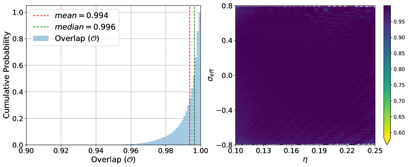
Using these conventions, we present overlap calculations between the target and predicted waveforms for the entire test data-set in Figure 6. To carry out these calculations, we used the plus and cross polarizations of the target waveforms spanning the range $t\in[-5000\textrm{M},130\textrm{M}]$. Our target waveforms consist of input data spanning the range $t\in[-5000\textrm{M},-100\textrm{M}]$ and complemented with our predicted waveforms that span the range $t\in[-100\textrm{M},130\textrm{M}]$. These calculations, presented in the top panels of Figure 6, indicate that both the mean and median overlaps ${\cal{O}}>0.99$, and that less than $10\%$ of the test dataset has ${\cal{O}}<0.98$. These outliers are localized at the edges of the parameter space, as shown in the top-right panel of Figure 6. In brief, our model predicts the late-inspiral, merger and ringdown waveform evolution in the time-range $[-100\textrm{M},130\textrm{M}]$. Since we sampled waveforms with a time step of $2\textrm{M}$, this means that the model outputs 115 steps of waveform evolution.

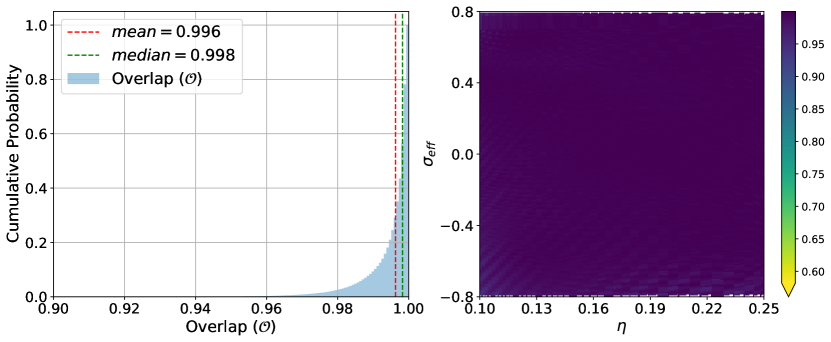
We have also used our AI model to quantify the accuracy of its predictions from two additional initial times, namely $t=\{-80\textrm{M},-60\textrm{M}\}$. In these cases, the model outputs 105 and 95 steps of waveform evolution, respectively. We present results for these cases in the mid and bottom panels of Figure 6. The overlap distributions for these cases are such that

• $t=-80\textrm{M}$: median and mean overlaps ${\cal{O}}>0.994$, with less than $6.1\%$ of the test dataset with ${\cal{O}}<0.98$.

• $t=-60\textrm{M}$: median and mean overlaps ${\cal{O}}>0.996$, with less than $2.4\%$ of the test dataset with ${\cal{O}}<0.98$.

We provide additional results that may be explored interactively in the website [44]. We see a progressive degradation in overlaps as we increase the target interval from $t\in[-60\textrm{M},130\textrm{M}]$ to $t\in[-100\textrm{M},130\textrm{M}]$. To explore the cause of this effect further, we trained three more models tasked with predicting only the segments $[-80\textrm{M},130\textrm{M}]$, $[-60\textrm{M},130\textrm{M}]$, and $[-50\textrm{M},130\textrm{M}]$ respectively. Let’s call these models M80, M60, and M50 respectively. Then we noticed that the performance of M60 was slightly worse than M80 when predicting the same segment $[-60\textrm{M},130\textrm{M}]$, and so on. This hints at some of the loss in performance coming from the margin effect, i.e., $-60\textrm{M}$ is at the margin during training for M60 but not for M80, etc. However, these small variations are hard to quantify due to inherent stochasticity of training deep neural networks. But more importantly, the most significant degradation in performance came from increasing the prediction span from $[-60\textrm{M},130\textrm{M}]$ to $[-80\textrm{M},130\textrm{M}]$, and similarly from $[-80\textrm{M},130\textrm{M}]$ to $[-100\textrm{M},130\textrm{M}]$.

Figure 6: Left column Cumulative distribution of overlaps between target and predicted waveforms. From top to bottom, we present results for our AI model predicting the waveform evolution from $t=\{-100\textrm{M},-80\textrm{M},-60\textrm{M}\}$, respectively. Right column Heatmap of the overlap distribution over the entire test set. We present results in terms of the symmetric mass-ratio and effective spin, $(\eta,\sigma_{\textrm{eff}})$, as defined in Equation (9).

Figure 7: Left panel Heatmap for one of the twelve cross attention heads showing which parts of the input waveform (shown in blue on the left) the decoder is paying attention to when predicting the output at any particular timestep (shown in green at the top). Right panel Heatmap showing one of the self attention heads of the decoder.

Interpretability: A nice side-effect and a major advantage of the attention mechanism is that it enables us to visualize and try to interpret what is happening inside the model. Looking at Equations (1) and (2) we notice that the coefficients $w_{ij}$ form a $t\times n$ matrix $A$. The $i^{th}$ row of $A$ consists of the attention scores over all the input vectors $\{x_{1},x_{2},x_{3},...,x_{n}\}$ when producing the $i^{th}$ output $h_{i}$, and hence each row sums up to $1$. Therefore visualizing the $i^{th}$ row of matrix $A$ shows which parts of the input $\{x_{1},x_{2},x_{3},...,x_{n}\}$ the model was “paying attention” to when generating the $i^{th}$ output $h_{i}$. Visualizing the whole matrix $A$ then summarizes where the model was “looking at” when generating each time-step of the output.

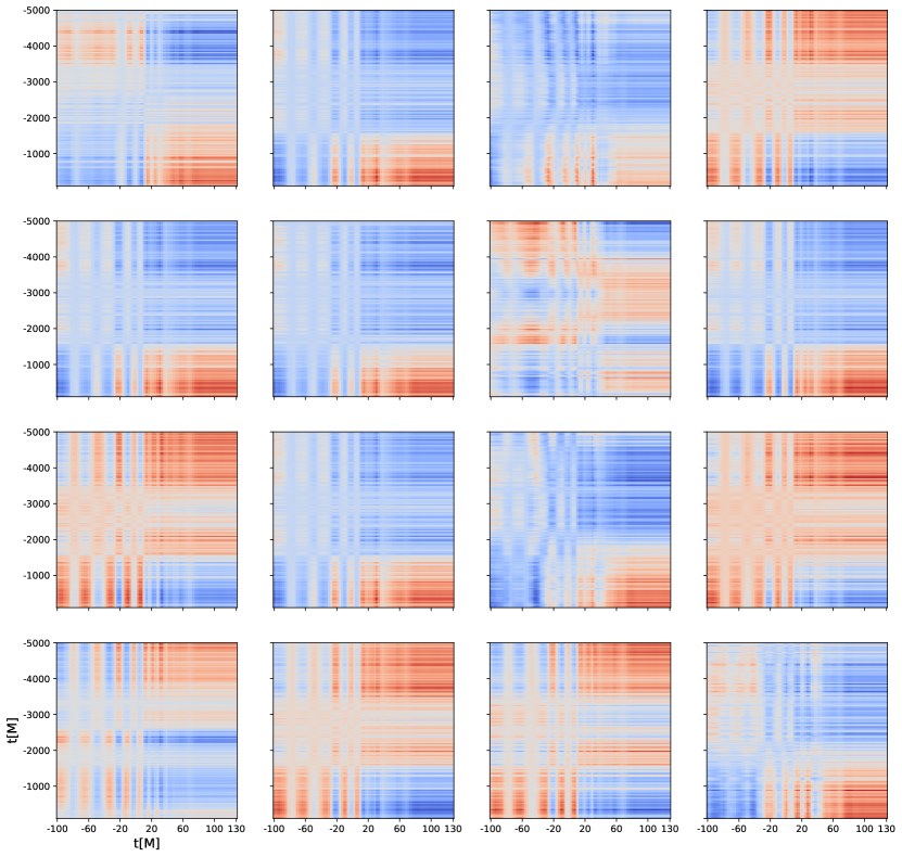
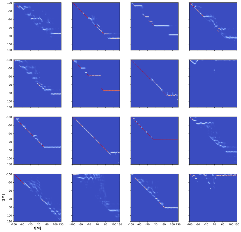
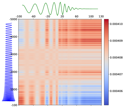
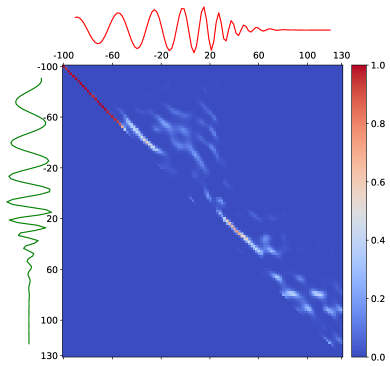
In this vein, we visualize the self-attention and cross-attention score matrices of the decoder module when generating the predictions for a sample waveform with parameters $\{q,s^{z}_{1},s^{z}_{2}\}=\{6.8,0.718,0.574\}$ in Figure 7. Therein we present results for one of the 12 attention heads from our model’s decoder. We present additional results for the other attention heads in Appendix B.

The left panel of Figure 7 shows the transpose of the cross-attention score matrix. Each column $j$ shows which parts of the input waveform segment ($t\in[-5000\,\textrm{M},-100\,\textrm{M}]$) the model was paying attention to when predicting the $j^{th}$ time-step of the target waveform segment ($t_{j}\in[-100\,\textrm{M},130\,\textrm{M}]$). For reference, we also plot the input waveform segment and the predicted waveform segment to the left and top of the matrix, respectively. We see that for the late-inspiral and merger phases of the prediction, the model is paying a diffused form of attention to the whole input segment, occasionally flip-flopping, i.e., paying more attention to the late-inspiral rather than early inspiral and vice versa. However, when predicting the ringdown, all of the attention gets focused towards the early inspiral of the input segment.

The right panel of Figure 7 shows the transpose of the self-attention matrix. Since predictions are generated autoregressively, the self-attention here is causal, i.e., at any given time-step $t=j$, the model cannot pay attention to future time-steps $t>j$. Consequently this matrix is upper triangular with a strong correlation between adjacent time-steps, thus mostly diagonal.

The results in Figure 7 provide a glimpse of the activity happening within our trained AI model that is responsible for accurate and reliable forecasting predictions. For the interested readers, we provide in the website [44] additional interactive results to enhance our intuition into how our AI model behaves for different astrophysical configurations.

IV Conclusions

We have designed an AI model that is capable of learning and predicting the late-inspiral, merger and ringdown evolution of quasi-circular, spinning, non-precessing binary black hole mergers. The data-driven methodology used to create these AI tools demonstrates that AI can learn and accurately describe the plus and cross polarizations of numerical relativity waveforms when we feed input signals that contain information up to $-100M$ before the merger event (defined as the amplitude peak of the waveform signal). We have also demonstrated that our AI model may forecast the waveform evolution starting at some other initial time $t_{i}$. In this study we presented quantitative results for the cases $t_{i}=-80\textrm{M}$ and $t_{i}=-60\textrm{M}$. In all these cases, the mean and median overlap between target and predicted waveforms is ${\cal{O}}\geq 0.99$.

We have also explored visualizing several components in our AI model (i.e., the various attentions heads) that are responsible for data-driven decision making and waveform forecasting. In particular, we generated visualizations to see which components of the input are responsible for the prediction of the pre-merger, merger and ringdown pieces of our predicted waveforms. We have made available an interactive website where users can explore these results in further detail for a variety of astrophysical systems. We expect that this approach persuades other researchers to go a step beyond and try to understand how AI models make predictions, and will help advance other efforts on creating interpretable AI models.

Appendix A Teacher Forcing

Our model is designed to predict the waveform evolution in the time range $-100\textrm{M}\leq t\leq 130\textrm{M}$. During both training and inference, we compute the loss and quantify the performance of the model by comparing the entire predicted and ground truth waveforms in the time segment $-100\textrm{M}\leq t\leq 130\textrm{M}$.

Figure 8: A visual representation of Teacher Forcing approach Top panel Teacher Forcing is used during training; at each time step the decoder is fed the ground truth target values from the previous time steps. Bottom panel During inference, Teacher Forcing is turned off, and at each time step the decoder is fed its own predicted values from the previous time steps.

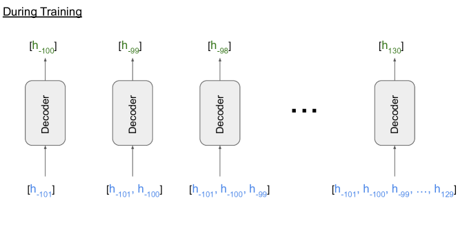
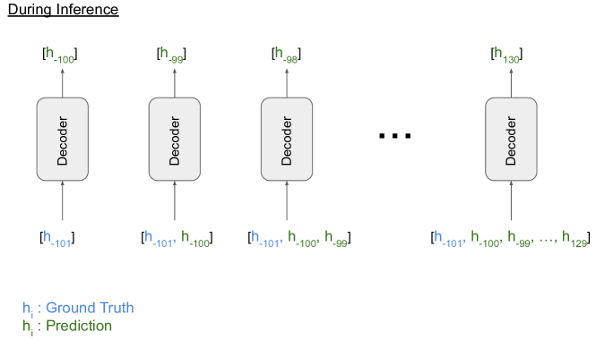
During both training and inference we feed the input waveform covering the time-span $[-5000\textrm{M},-100\textrm{M}]$ into the encoder. Additionally, during training we also employ Teacher Forcing, whereby at each time step the decoder is fed the ground truth target values from the previous time steps, as illustrated in the top panel of Figure 8. This methodology results in a more stable training and helps the model converge faster. Finally, during inference we turn off Teacher Forcing and instead feed the decoder its own predictions from the previous time-steps, as illustrated in the bottom panel of Figure 8.

Appendix B Interpretability

We provide additional results for the 12 attention heads that our AI model utilizes for the forecasting of numerical relativity waveforms. As in Figure 7, we have produced these results for a binary black hole system with parameters $\{q,s^{z}_{1},s^{z}_{2}\}=\{6.8,0.718,0.574\}$. For additional results, we refer readers to the interactive website [44].

Figure 9: Response of all cross attention heads to a given input signal, indicating which parts of the input waveform signal are taken into account to forecast the late-inspiral, merger and ringdown evolution. This behaviour is very consistent across the parameter space under consideration.

Figure 10: As Figure 9 but now for self attention heads.