Non-standard modeling of a possible blue straggler star, KIC 11145123

Abstract

Non-standard modeling of KIC 11145123, a possible blue straggler star, has been asteroseismically carried out based on a scheme to compute stellar models with the chemical compositions in their envelopes arbitrarily modified, mimicking effects of some interactions with other stars through which blue straggler stars are thought to be born. We have constructed a non-standard model of the star with the following parameters: $M=1.36M_{\odot}$, $Y_{\mathrm{init}}=0.26$, $Z_{\mathrm{init}}=0.002$, and $f_{\mathrm{ovs}}=0.027$, where $f_{\mathrm{ovs}}$ is the extent of overshooting described as an exponentially decaying diffusive process. The modification is down to the depth of $r/R\sim 0.6$ and the extent $\Delta X$, which is a difference in surface hydrogen abundance between the envelope-modified and unmodified models, is $0.06$. The residuals between the model and the observed frequencies are comparable with those for the previous models computed assuming standard single-star evolution, suggesting that it is possible that the star was born with an relatively ordinary initial helium abundance of $\sim 0.26$ compared with that of the previous models ($\sim 0.30$–$0.40$), then experienced some modification of the chemical compositions, and gained helium in the envelope. Detailed analyses of the non-standard model have implied that the elemental diffusion in the deep radiative region of the star might be much weaker than that assumed in current stellar evolutionary calculations; we need some extra mechanisms inside the star, rendering the star a much more intriguing target to be further investigated.

1 Introduction

Space-borne missions such as Kepler (Koch et al., 2010) and TESS (Ricker et al., 2014) have enabled us to conduct extremely precise measurements of stellar variabilities ($\sim$ $10^{-5}$ magnitude) with short cadences ($\sim$ minutes) and long durations ($\sim$ months to years). In particular, asteroseismology, a branch of stellar physics in which we probe the interiors of stars based on the measurements of stellar oscillations (e.g. Aerts et al., 2010), has been greatly benefitting from such high-quality observations carried out by the modern spacecrafts, and we are now able to perform asteroseismic analyses to identify evolutionary stages (e.g. Bedding et al., 2011; Chaplin and Miglio, 2013) and to investigate internal structures (e.g. Kosovichev and Kitiashvili, 2020) and dynamics (e.g. Aerts et al., 2019) of stars in detail, shedding new light on the understanding of stellar interiors from the observational point of view.

Among stars thus asteroseismically analyzed so far, KIC 11145123, which is one of the Kepler targets and photometrically categorized as a main-sequence A-type star (Huber et al., 2014), outstands in terms of its well-resolved frequency splittings for p, g, and mixed modes, whose restoring forces are pressure, buoyancy (gravity), and either of them (depending on where the modes are established), respectively (see, e.g., Unno et al., 1989). The well-determined frequencies and frequency splittings have allowed us to perform a number of detailed asteroseismic analyses of the star inferring, for instance, the internal rotation profile (Kurtz et al., 2014; Hatta et al., 2019), the asphericity (Gizon et al., 2016), and the evolutionary stage of the star (Kurtz et al., 2014; Takada-Hidai et al., 2017). It should be instructive to note that the number of main-sequence stars in Kepler targets which exhibit well-resolved frequency splittings for both p and g modes is just three (Saio et al., 2015; Schmid and Aerts, 2016) including KIC 11145123; the star therefore could be an important testbed which may be helpful for putting observational constraints on theoretical studies of the stellar interiors.

There is, however, an issue on previous equilibrium models and the thus identified evolutionary stage of the star (Kurtz et al., 2014; Takada-Hidai et al., 2017). Kurtz et al. (2014) is the first to construct a 1-dimensional model of the star to reproduce the observed frequencies via Modules for Experiments in Stellar Astrophysics (MESA; version 4298, Paxton et al., 2013) and they noticed that higher initial helium abundance of $\sim 0.3$–$0.4$ is much favored. But such higher initial helium abundance is difficult to explain for a simple single star considering the ordinary stellar evolution, and thus, we need some mechanisms to render the helium abundance of the star so high.

One simple scenario is that the star experienced some interactions with other stars such as mass accretion, stellar merger, or stellar collision, and it has obtained extra helium from the outside. Interestingly, the inferred internal rotation profile of the star, where the outer envelope is rotating slightly faster than the deep radiative region (Kurtz et al., 2014; Hatta et al., 2019), is also pointing toward the same scenario; we need some mechanisms of angular momentum transfer, probably from the outside, to realize the inferred rotational profile, and interacting with other stars can be a straightforward explanation. Based on the suggestion that the star has experienced some interactions during the evolution, in addition to the relatively lower initial metallicity of $\sim 0.010$ determined by asteroseismic modeling of the star, Kurtz et al. (2014) finally pointed out that the star could be a blue straggler star (Sandage, 1953), which is a kind of stars thought to be born via binary interactions or stellar collisions (Boffin et al., 2015) and appears somehow rejuvenated compared with other stars at the same age.

To better comprehend properties of a star from a different perspective, Takada-Hidai et al. (2017) have conducted the spectroscopic observation of the star with Subaru/HDS. They firstly found that the star has a sub-solar iron content $[\mathrm{Fe}/\mathrm{H}]\sim-0.7$ which approximately corresponds to $Z\sim 0.003$. Based on the low metallicity, which was below the parameter range surveyed by Kurtz et al. (2014), they have modeled the star assuming single-star evolution, resulting in the initial helium abundance as high as that of Kurtz et al. (2014); the situation has not improved. Importantly, however, based on the abundance pattern of the star, they found the star to be spectroscopically a blue straggler star as suggested by Kurtz et al. (2014). The star has probably experienced some interactions with other stars, which could be a reason for the high initial helium abundance previously deduced via modeling the star assuming single-star evolution; there is room for modeling the star in a non-standard manner where we take such interactions with other stars during the evolution into account.

The primary goal of this paper is to construct a 1-dimensional non-standard model of a possible blue straggler star, KIC 11145123, taking into account effects of some interactions with other stars. Though there have been numerous attempts of non-standard modeling of blue straggler stars (e.g. Brogaard et al., 2018), this is the first time such non-standard modeling of blue straggler stars has been carried out asteroseismically. In addition, the non-standard model would be of a great value since we can further perform detailed analyses such as rotation inversion of the star (Hatta et al. in prep.)

As a first step toward the goal described in the previous paragraph, we specifically concentrate on effects of modifications of chemical compositions, namely, helium enhancements, in the envelope caused by whatever can lead to such envelope modification. In other words, we do not consider detailed physics concerning specific processes such as mass accretion or stellar merger, and what we do consider is just the resultant effects of these processes on stellar structure. Since there has been no scheme to realize such computations to our knowledge, we would like to develop the scheme in this study, which is actually the minor (though necessary) goal in this study.

It is also worth mentioning that there do exist single stars with high initial helium abundances of $0.30$–$0.40$ which are thought to be born in such high helium environments contaminated by stellar winds from already existing asymptotic giant branch stars. This multiple main-sequence phenomenon (Bastian and Lardo, 2018) has been recently observed for some globular clusters. Although KIC 11145123 is currently not considered as such a peculiar single star based on the chemical abundance pattern and the kinematics determined by Takada-Hidai et al. (2017), we can further deepen the discussion about the evolutionary history of the star from a different perspective by constructing a non-standard model of the star, comparing the non-standard model with the previous (standard) models, and finally assessing whether the initial helium abundance of the star was really high or not.

The structure of this paper is as follows. After we briefly explain general setups for computing stellar models and frequencies in Section 2, a scheme of calculating 1-dimensional stellar models, whose chemical compositions are arbitrarily modified, and examples of envelope-modified models computed via the scheme are presented in Section 3. Because the scheme is newly developed, we demonstrate the concept and the mathematical formulations in detail. In Section 4, the non-standard model of the star is obtained by applying the scheme explained in Section 3. Section 5 is devoted to discussions on the evolutionary stage, the internal structure, and a possible relation between the internal structure and the rotational velocity shear, the latter of which has been inferred by Hatta et al. (2019). We conclude in Section 6.

2 Numerical codes

Stellar models are computed via MESA (version 9793, Paxton et al., 2015). Neither rotation nor magnetic fields is assumed in the computation. The OPAL tables are used for both the equation of state and the opacity, and the nuclear reaction rate is obtained by interpolation based on a built-in table in MESA, called ‘basic.net’.

As mixing processes during the evolution, convection, convective overshooting, and elemental diffusion are activated. The free parameter in the Mixing Length Theory $\alpha_{\mathrm{MLT}}$ is fixed to be $1.7$ following Kurtz et al. (2014). Convective overshooting is implemented as a diffusive process whose diffusion coefficient follows an exponential decay above the convective boundary (Herwig , 2000). The effect of elemental diffusion is incorporated into the evolutionary calculation by solving so-called Burger’s equation which is based on Boltzman’s equation in kinematics (Burgers, 1969). In our calculations, radiative levitation is not included. Note that though the scheme for elemental diffusion is considered to be working well for models with $\sim 1M_{\odot}$, it has been long pointed out that the scheme often overestimates the diffusion velocity of helium in the outermost layer of models with $>1.3M_{\odot}$, sometimes leading to the depletion of helium there, which has not been observationally confirmed (Morel and Thevenin, 2002). To avoid such depletion of helium in the outermost layer of the models, a special scheme $\mathrm{radiation}\_\mathrm{turbulence}\_\mathrm{coeff}$ (Morel and Thevenin, 2002) is turned on and set to be unity in our computations. For more details, see a series of papers about the code (Paxton et al., 2011, 2013, 2015, 2018, 2019).

Eigenfrequencies of stellar models are computed via linear oscillation code GYRE (Townsend and Teitler, 2013). The effects of rotation, magnetic fields, asphericity, and nonadiabaticity on the eigenoscillations of a certain model are not taken into account; these effects are considered to be sufficiently small for the star (e.g. Kurtz et al., 2014).

3 Method

In this section, a scheme of constructing 1-dimensional stellar models whose chemical compositions are arbitrarily modified is presented. The scheme is formulated similarly to the linear adiabatic radial oscillation of stars. Since the scheme is new (though the scheme itself is simple enough for us to incorporate it with the existing codes such as MESA), we demonstrate the concept (Section 3.1), the mathematical formulations (Section 3.2), and examples of modified models and the frequencies computed via the scheme (Section 3.3) in detail. We see the applications of the scheme to the non-standard modeling of KIC 11145123 in Section 4.

Before going into details, we have two specific notes as follows. Firstly, in this section, we explain the scheme only focusing on envelope-modification for simplicity. This is because such envelope-modification is the central topic throughout most of this paper. It is however possible for us to consider modifications of chemical compositions in regions other than the envelope; one of such applications can be found in Subsection 5.2.1 and Section 5.3, where not the envelope but the deep radiative region is modified to render the chemical composition gradient be artificially steeper.

Secondly, in this study, envelope-modified models are constructed by exchanging hydrogen for helium (mimicking helium enhancements in the envelope) so that the total mass is fixed, i.e. $\delta M=0$. Therefore, we should be aware that an unmodified model is not identical to a progenitor of envelope-modified models. On the other hand, the fixed total mass enables us to simplify the non-standard modeling of the star, and we can carry out g-mode and p-mode fittings independently from each other as will be shown in Section 4. We discuss the point later again in Section 5.1 as well.

3.1 Concept for envelope-modifying scheme

Generally speaking, a model of a star at a certain age is considered as a sphere whose interior is divided into multiple spherical layers called mass shells. The mass inside the concentric sphere $m$ is often taken as an independent variable. Dependent variables as functions of $m$ (strictly speaking, they are also functions of time which is assumed to be fixed here), namely, the distance from the center of the star $r$, the pressure $P$, the temperature $T$, the local luminosity $l$, and the mass fractions for each chemical element $X_{i}$ (the index $i$ represents each chemical element), together with other parameters such as the thermodynamic quantities (the density $\rho$, the adiabatic sound speed $c^{2}$, etc.), the opacity $\kappa$, and the nuclear energy generation rate $\varepsilon$ are assigned for each mass shell so that the set of the equations for stellar structure and evolution (see, in particular, Section 6 in Paxton et al., 2011) is satisfied with the variables above with certain precisions. This is the standard view of a stellar model, and let us call this the model $M_{0}$ (see Figure 1).

Then, how do we model the processes of the chemical composition modification, which is possibly caused by, for instance, mass accretion, and incorporate the effects on the structural variables $(r,P,T,l,X_{i})$ of the stellar model $M_{0}$ defined in the last paragraph? We simplify the processes with four steps as described in the following paragraphs.

Figure 1: Schematic view of the three models and the relations among them.

First, we determine a particular mass shell in the model above which the chemical compositions $X_{i}$ are to be changed. The amount of the modification to $X_{i}$ is arbitrary, and an example of the explicit forms for the amount is given in Section 3.3 as a function of $m$. We fix the structural parameters other than $X_{i}$ (namely, $r$, $P$, $T$, and $l$). The thermodynamic parameters, the opacity, and the nuclear energy generation rate are accordingly changed based on the already computed tables such as OPAL. Note that there are usually two degrees of freedom in terms of the variation in thermodynamic quantities when $X_{i}$ are changed. In this study, the density $\rho$ (in other words, the distance of the mass shell from the center $r$) and the temperature $T$ are assumed to be fixed. We can instead select the other sets of parameters to be fixed, for example, the specific entropy $s$ and the density $\rho$, which nevertheless do not strongly affect the final results in this study.

The modification introduced in the first step results in the change of the mean molecular weights $\mu$ of the modified mass shells, also leading to the change of the pressure $P$. This spherical model $M_{0}$ is thus no longer in hydrostatic equilibrium state; the hydrostatic equation is not satisfied with the new set of modified parameters (remember that $r$ is assumed to be fixed, and thus the gravitational force is not changed though the pressure gradient is). Let us call this model the perturbed model $M_{0}^{\prime}$ (see Figure 1).

Then, the perturbed model $M_{0}^{\prime}$ should start radially oscillating motions around a particular hydrostatic equilibrium point. Based on the assumption of the adiabatic process for the oscillating motions (which can be partly justified because the dynamical timescale is usually much smaller than the thermal relaxation timescale for a main-sequence star), there is one unique equilibrium point, and we adopt the point as the envelope-modified model (denoted as $M_{1}$ in Figure 1). Specifically, the model $M_{1}$ can be obtained by 1) solving the second order differential equation which is similar to that for the linear adiabatic radial oscillation except that the acceleration term is replaced with the deviation from the hydrostatic equilibrium (see Section 3.2) and 2) subtracting the thus determined radial displacements from the radial coordinates of the perturbed model $M_{0}^{\prime}$. This is the second step.

In the second step, the modification is implicitly assumed to be small enough that we can treat the modification as a perturbation, which is required to guarantee the validity of the radial displacements determined by solving the linear differential equation. Therefore, to obtain a model whose outer region is significantly modified compared with the unperturbed model $M_{0}$, we have to repeat the step 1 and 2 substantial times. We denote the model obtained in this way as $M_{1}^{\prime}$.

Finally, because the model $M_{1}^{\prime}$ is considered to have deviated from a thermal equilibrium state, we have to resettle the model again toward a thermal equilibrium state. This final step can be done by, in this study, further evolving the model $M_{1}^{\prime}$ for the corresponding thermal relaxation timescale of $\sim$ a few million years so that the resettled model satisfies the equation of the energy conservation and the equation for the temperature gradient.

3.2 Formulation

The mathematical formulations to describe the steps in the previous section are presented in this section. Let us start with the set of equations for stellar structure which the parameters of the unperturbed model $M_{0}$ satisfy, expressed as below:

$$\frac{dP_{0}}{dm}=-\frac{Gm}{4\pi r_{0}^{4}},$$ (1)

$$\frac{dr_{0}}{dm}=\frac{1}{4\pi r_{0}^{2}\rho_{0}},$$ (2)

$$\frac{dT_{0}}{dm}=-\frac{Gm}{4\pi r_{0}^{4}}\frac{T_{0}}{P_{0}}\nabla_{0},$$ (3)

and

$$\frac{dl_{0}}{dm}=\varepsilon_{n,0}-\varepsilon_{\nu,0},$$ (4)

where the subscripts $0$ are representing the unperturbed state of the model $M_{0}$. The actual temperature gradient $\nabla_{0}$ is defined as $d\,\mathrm{ln}\,T_{0}$/$d\,\mathrm{ln}\,P_{0}$. The other parameters have the same meaning as in the last section.

In the first step, the outer envelope is modified, i.e. we artificially add a small perturbation to the chemical composition $\mu$ of the unperturbed model $M_{0}$

$$\mu_{0}\to\mu_{1}=\mu_{0}+\delta\mu.$$

It is totally up to us to decide how to modify the envelope. In this study, as shown in Section 3.3, we exchange hydrogen with helium so that the total mass $M$ is unchanged. The corresponding explicit form for $\delta\mu$ is given there.

We also assume that the temperature and the density are the same as those of the starting model $M_{0}$. Based on these assumptions, we can calculate the perturbed pressure $P_{\rm{md}}$ by interpolating tables of equation of state such as OPAL,

$$P_{0}=P(\rho_{0},T_{0},\mu_{0})\to P_{\mathrm{md}}=P(\rho_{0},T_{0},\mu_{1}).$$

It is then obvious that the perturbed model $M_{0}^{\prime}$ is not in a hydrostatic equilibrium state as described in Section 3.1.

In the second step, we consider that the deviation from the hydrostatic equilibrium state is caused by adding the radial displacement $\xi_{r}$ to another hydrostatic equilibrium model $M_{1}$ (see Figure 1). The structural parameters of the model $M_{1}$ must satisfy the hydrostatic equation:

$$\frac{dP_{1}}{dm}=-\frac{Gm}{4\pi r_{1}^{4}},$$ (5)

where the subscripts $1$ are representing the model $M_{1}$. We can relate the new parameters to those of $M_{0}^{\prime}$ as

$$r_{1}=r_{0}-\xi_{r},$$ (6)

$$P_{1}=P_{\rm{md}}-\delta P,$$ (7)

$$T_{1}=T_{0}-\delta T,$$ (8)

and

$$\rho_{1}=\rho_{0}-\delta\rho.$$ (9)

If we substitute relations (6) to (9) for expression (5), we have the following equation

$$\frac{d(P_{\rm{md}}-\delta P)}{dm}=-\frac{Gm}{4\pi(r_{0}-\xi_{r})^{4}}.$$ (10)

Note that we are not considering perturbed equations for the temperature gradient, because we concentrate on the adiabatic process, as it is explained later. The equation of the energy conservation is also not considered here due to the assumption that the local luminosity $l$ is fixed. See Section 3.1 for how to handle possible deviations from the thermal equilibrium states.

Assuming that the perturbations are small enough to justify neglecting the perturbed quantities of higher than the first order, the equation above can be further simplified as below:

$$-\frac{d(\delta P)}{dm}=-\frac{Gm}{4\pi r_{0}^{4}}\frac{4\xi_{r}}{r_{0}}-\delta h,$$ (11)

where $\delta h$ is defined as

$$\delta h\equiv\frac{dP_{\rm{md}}}{dm}+\frac{Gm}{4\pi r_{0}^{4}},$$ (12)

which represents a degree of deviation from a hydrostatic equilibrium.

The perturbed (thermodynamic) quantities are dependent on how we take the pathway from $M_{1}$ to $M_{0}^{\prime}$. We discuss the simplest way where the adiabatic process is assumed. In the adiabatic process, there is no heat transfer among the mass shells of the model. We can relate the small perturbations of the thermodynamic quantities such as $\delta P$, $\delta T$, and $\delta\rho$ to their values $P_{\rm{md}}$, $T_{0}$, and $\rho_{0}$ with adiabatic exponents as follows:

$$\frac{\delta P}{P_{\rm{md}}}=\Gamma_{1}\frac{\delta\rho}{\rho_{0}}$$ (13)

and

$$\frac{\delta T}{T_{0}}=(\Gamma_{3}-1)\frac{\delta\rho}{\rho_{0}},$$ (14)

where the two adiabatic exponents are defined as

$$\Gamma_{1}\equiv\biggl{(}\frac{\partial\ \rm{ln}\ \it{P}}{\partial\ \rm{ln}\ \rho}\biggr{)}_{\rm{ad}}$$

and

$$\Gamma_{3}-1\equiv\biggl{(}\frac{\partial\ \rm{ln}\ \it{T}}{\partial\ \rm{ln}\ \rho}\biggr{)}_{\rm{ad}},$$

and they can be obtained from tables for equation of state.

When we insert expression (13) into equation (11), it can be rewritten as

$$-\frac{d}{dm}(c^{2}_{\rm{md}}\delta\rho)=-\frac{Gm}{4\pi r_{0}^{4}}\frac{4\xi_{r}}{r_{0}}-\delta h.$$ (15)

The adiabatic sound speed for the model $M_{0}^{\prime}$ is expressed as $c^{2}_{\rm{md}}$. Let us then consider the mass conservation in the case of the linear oscillation, namely,

$$\rho^{\prime}+\nabla\cdot(\rho_{0}\boldsymbol{\xi})=0,$$

based on which we can relate the density perturbation $\delta\rho$ to the radial displacement $\xi_{r}$ in the following way

$$\delta\rho=-\rho_{0}\frac{1}{r_{0}^{2}}\frac{d}{dr_{0}}(r_{0}^{2}\xi_{r}).$$ (16)

We have used a relation between the Eulerian perturbation ($\rho^{\prime}$) and the Lagrangian perturbation ($\delta\rho$), and we adopt the spherical coordinate to articulate the specific form of the differentiation. For the convenience in later discussions, we express the differentiation in expression (16) in terms of the mass coordinate using the expression (2)

$$\delta\rho=-\frac{2\rho_{0}}{r_{0}}\xi_{r}-4\pi r_{0}^{2}\rho_{0}^{2}\frac{d\xi_{r}}{dm}.$$ (17)

Combining the expressions (15) and (17), we finally have a linear differential equation for the radial displacement $\xi_{r}$ in the case of the adiabatic process as follows:

$$4\pi r_{0}^{2}\rho_{0}^{2}c_{\rm{md}}^{2}\frac{d^{2}\xi_{r}}{dm^{2}}+\biggl{[}\frac{d}{dm}(4\pi r_{0}^{2}\rho_{0}^{2}c_{\rm{md}}^{2})+\frac{2\rho_{0}c_{\rm{md}}^{2}}{r_{0}}\biggr{]}\frac{d\xi_{r}}{dm}$$

$$+\biggl{[}\frac{d}{dm}\biggl{(}\frac{2\rho_{0}c_{\rm{md}}^{2}}{r_{0}}\biggr{)}+\frac{Gm}{\pi r_{0}^{5}}\biggr{]}\xi_{r}+\delta h=0,$$

(18)

with the following boundary conditions

$$\xi_{r}=0\,\,\,(\mathrm{at\,the\,center})$$ (19)

$$\delta P=0\,\,\,(\mathrm{at\,the\,surface}),$$ (20)

the latter of which is the so-called zero boundary condition.

Equation (18) can be numerically solved under the boundary conditions (19) and (20) when we have all the properties of the perturbed model $M_{0}^{\prime}$. We can compute the density perturbation $\delta\rho$ based on expression (17), and subsequently, the temperature perturbation $\delta T$ based on expression (14). Because the differential equation has been the linearization of the perturbed equation (10), we have to iterate the procedure explained above.

After we resettle the perturbed model with one perturbation in the mean molecular weight, we just repeat the same procedure until we obtain the model whose envelope is as modified as we would like to as is shown later in Section 3.3. There are thus no special mathematical formulations in the third step and the fourth step.

3.3 Envelope-modified models and the frequencies

In this section, we present examples of envelope-modified models, which are characterized by helium enhancements in the envelopes, computed based on the scheme explained in the preceding section. We also show eigenfrequencies of the envelope-modified models and a relation between extents of the helium enhancement and corresponding frequency variations, which are to be utilized in the non-standard modeling of the star as will be seen in Section 4.

The basic settings for the calculation follow. First, we prepare an unperturbed model. The mass and the initial helium abundance are $1.30M_{\odot}$ and $0.260$. The metallicity is $0.003$, and it is unaltered during the envelope-modification. The age of the model is determined based on the asymptotic value of the g-mode period spacing $\overline{\Delta P_{\mathrm{g}}}$ which has been frequently used as an indicator for stellar evolutionary stages (see, e.g., Unno et al., 1989; Aerts et al., 2010); the evolutionary calculation is stopped when $\overline{\Delta P_{\mathrm{g}}}$ (one of the outputs of MESA, computed based on the integration of the $\rm{Brunt}$-$\rm{{V\ddot{a}is\ddot{a}l\ddot{a}}}$ frequency of the model) is $2100\,\mathrm{s}$, which is close to the mean value of the observed g-mode period spacing for KIC 11145123, $2070\,\mathrm{s}$ (Kurtz et al., 2014). The extent of overshooting $f_{\mathrm{ovs}}$ (see the definition, for example, in Section 5 of Paxton et al., 2011) is set to be 0.014, which is around the typical values for $f_{\mathrm{ovs}}$. The diffusion process is activated. The default settings in MESA are used for the other prescriptions. The parameters determined in the above are mostly based on the previous models of KIC 11145123 (Kurtz et al., 2014; Takada-Hidai et al., 2017).

Figure 2: Examples of the modifications in the hydrogen mass fraction computed following the equation (21), with different abscissas, namely, the fractional radius $r/R$ (top) and the fractional mass $m/M$ (bottom). Four ways of modification are shown changing the parameters $\alpha$ and $\beta$. The parameter $m_{\mathrm{c}}$ is fixed to be $0.99976$. It is seen that as $\beta$ increases the amount of the modification increases as well. Increasing $\alpha$ leads to the wider transition from the unperturbed region to the perturbed one.

Then, the envelope-modifying scheme is applied to the model. The differential equation (18) is solved under the zero boundary conditions (19) and (20) based on the second-order implicit scheme where the staggered mesh is adopted to describe the quantities and their derivatives (see Figure 9 in Paxton et al., 2011). We parameterize the modification (hydrogen depletion or helium enhancement) in the following way:

$$\delta X\equiv X_{\mathrm{md}}-X_{0}=-\beta\times\biggl{(}\mathrm{tanh}\biggl{(}\frac{m-m_{\mathrm{c}}}{\alpha}\biggr{)}+1\biggr{)},$$ (21)

in which $X_{\mathrm{md}}$ and $X_{0}$ are hydrogen mass fractions for the perturbed model $M_{0}^{\prime}$ and the unperturbed model $M_{0}$ (see Figure 1). There are three free parameters in the expression (21), namely, $\beta$, $\alpha$, and $m_{\mathrm{c}}$ which determine the extent, the width of a transition, and the depth of the modification, respectively (see Figure 2). Note that the modification in the helium mass fractions $\delta Y$ is given as $-\delta X$ so that the sum of the mass fractions remains to be unity. It should be also noted that what we practically perturb is not the mean molecular weights $\mu$ but the hydrogen mass content $X$.

In this section, we express one modification with the following parameters: $\alpha=7.5\times 10^{-4}$, $\beta=5\times 10^{-6}$, and $m_{\mathrm{c}}=0.99976$. The modification is added to the unperturbed model $4\times 10^{4}$ times, and models perturbed $10^{4}$, $2\times 10^{4}$, $3\times 10^{4}$, and $4\times 10^{4}$ times are preserved for calculations of the eigenfrequencies. It has been confirmed that $\delta h$ of the envelope-modified models is at most of the order of $10^{-6}$ which is almost the same as those for ordinary stellar models computed via MESA, validating that our scheme is correctly working. The calculation of eigenfrequencies is via GYRE (Townsend and Teitler, 2013).

Figure 3: Modified hydrogen fractions (left) and the corresponding p-mode eigenfrequencies (right). The envelope-modified models (left) are obtained after $10^{4}$ (blue), $2\times 10^{4}$ (turquoise), $3\times 10^{4}$ (gold), and $4\times 10^{4}$ (red) times perturbations. The unperturbed profile is also indicated (black). The hydrogen abundance decreases more as the envelope is perturbed more, where $10^{4}$ times perturbations approximately correspond to the decrease in the surface hydrogen abundance $\Delta X\sim 0.07$. P-mode eigenfrequencies for radial modes (blue), dipole modes (red), and quadrupole modes (green) are shown for each perturbed model in the right panels. It is seen that the more the envelope is modified, the more the p-mode frequencies are shifted, as expected. The frequency range is chosen based on the observed p-mode frequencies of KIC 11145123 (see also Table 4 of Kurtz et al., 2014).

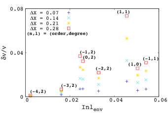
Figure 4: Relative frequency variation, defined as $\delta\,\mathrm{ln}\,\nu_{ij}=(\nu_{ij}-\nu_{0j})/\nu_{0j}$, against the corresponding envelope mode inertia, defined in the expression (22), computed based on the envelope-modified models which are here represented by the surface hydrogen abundance difference $\Delta X\sim 0.07$ (blue), $0.14$ (turquoise), $0.21$ (gold), and $0.28$ (red). (see also Figure 3). The radial order and spherical degree of each mode are presented as well. Detailed meanings of the indices can be found in the text. Rough proportionality of the relative frequency variation with respect to the extent of modification can be confirmed. A positive correlation, though non-monotonic, between the relative frequency variation and the envelope mode inertia is also seen, which is discussed in the text.

Results of the computations are presented in Figure 3. It is evident that the hydrogen is less abundant as the envelope is modified more (see the left panel of Figure 3). Some of the computed abundance profiles exhibit the inversion in the mean molecular weight due to the envelope modification (see cyan, yellow, and red curves in the left panel of Figure 3), but, in our settings for MESA, it has been confirmed that the modified profiles are stable at least for the thermal timescale. Moreover, implementing mixing processes which work in the presence of mean molecular weight inversions with the thermal timescale (such as thermohaline mixing) does not change results of the non-standard modeling of KIC 11145123 significantly. We therefore do not further discuss the point in this study.

The hydrogen decrease represented by $\Delta X$ in Figure 3 (or, the helium enhancement) brought about by the envelope modifications should affect the adiabatic sound speed in the envelope. The p-mode frequencies, which are strongly dependent on the adiabatic sound speed (see, e.g., Unno et al., 1989), are thus varying as we perturb the envelope more (see the right panels in Figure 3). Interestingly (and importantly), the amounts of the frequency variations are, roughly speaking, proportional to the amounts of the modification, though the dependence should be non-linear. In addition, the amounts of the frequency variations are different from mode to mode, which is readily confirmed when we see the right panels in Figure 3 (compare, for instance, the blue bar and the red bars). We present a further discussion on that point in the following paragraphs, since these features help us reduce the size of the grid with which the non-standard modeling is carried out as we will see later in Section 4.2.

To see relations between the amounts of frequency variations and the mode properties more clearly, we plot, in Figure 4, the relative frequency variation, defined as $\delta\,\mathrm{ln}\,\nu_{ij}=(\nu_{ij}-\nu_{0j})/\nu_{0j}$, against the corresponding “envelope mode inertia” which is defined as below:

$$I_{j}^{\mathrm{env}}=\int_{\mathrm{env}}\rho|\boldsymbol{\xi}_{j}|^{2}dV,$$ (22)

where the indices $i$ and $j$ stand for the extent to which a model is modified ($\Delta X\sim 0.07$, $0.14$, $0.21$, and $0.28$, in this case) and a particular mode, respectively. The unperturbed model is designated as $i=0$, and the eigenvector of the mode is expressed as $\boldsymbol{\xi}_{j}$. The envelope mode inertia is computed by integrating $\rho|\boldsymbol{\xi}_{j}|^{2}$ in the part of the envelope determined by us beforehand (here, the envelope is defined as a region $r/R>0.7$). Note that the total mode inertia (obtained by carrying out the integration throughout the model) is normalized to be $1/4\pi$.

Strictly speaking, we can describe the frequency variations based on the structure kernels of the unperturbed model and the structural differences caused by the modifications. But this is not the case here because the modifications are too large to consider them as small perturbations and apply the first-order perturbation theory to explain the frequency variations, which is the reason why we, as a rough approximation, have chosen $I_{j}^{\mathrm{env}}$ instead of structure kernels as an indicator for the sensitivity to the envelope modifications (Figure 4). It is seen that, for a given envelope mode inertia, the relative frequency variation is proportional to the extent of modification. We can also see that, for a particular extent of modification (see, e.g., a series of red squares in Figure 4), the relative frequency variation increases (though not exactly monotonically) as the envelope mode inertia increases, which is understandable because the chemical composition modification in the envelope does not affect properties of a mode if the mode does not have sensitivity (which is represented by the envelope mode inertia) in the modified envelope.

It should be instructive to mention that we can qualitatively explain the non-monotonic trend seen in Figure 4 by checking the mode inertia densities $\rho|\boldsymbol{\xi}_{j}|^{2}r^{2}$ of the unperturbed model. For example, the inertia density of the mode with $(n,l)=(1,1)$ is maximum around $r/R\sim 0.95$ which is included in a region most affected by the modifications, leading to the larger frequency variation compared with those of the other modes such as modes with $(n,l)=(-2,2)$ and $(-1,1)$ whose mode inertia densities are maximum around $r/R\sim 0.8$ where the structure is less perturbed than that around $r/R\sim 0.95$, leading to the relatively smaller frequency variations. We however do not attempt to explain all the non-monotonic signatures in Figure 4 not only because, as shown in Section 4, assuming the rough proportionality in the non-standard modeling is sufficient to obtain a reasonable envelope-modified model of KIC 11145123 but also because taking the non-monotonic trend into account has little impact on the final inference of the non-standard modeling.

Finally, we would like to mention that g-mode frequencies are almost insensitive to envelope modifications; the g-mode frequencies of the envelope-modified models are mostly the same. This is because g modes mainly propagate through the deep radiative region (see, e.g., Unno et al., 1989) and their envelope mode inertias are almost zero. The properties of g- and p-mode frequency variations with respect to envelope modifications are to be utilized in Section 4 where asteroseismic non-standard modeling of KIC 11145123 is performed.

4 Non-standard modeling

We have three steps in the non-standard modeling of the star as below. First, we compute ordinary models via MESA to fit atmospheric parameters with a relatively coarse grid (Section 4.1). Then, a finer grid is constructed based on the results of the coarse-grid-based modeling to compute models reproducing g-mode frequencies (Section 4.2). Finally, we modify the envelopes of the models by increasing helium mass contents in the envelopes to fit p-mode frequencies (Section 4.3). Such independent modeling can be achieved when, as we see in Section 3.3, the structures of the deep regions are not affected much during the envelope modifications. For each section, we present the specific procedures, the parameter ranges, and the results.

4.1 Coarse-grid-based modeling

4.1.1 Specific procedures

We firstly prepare the following grids of parameters: mass $M$ ($1.1$–$2.1M_{\odot}$, with the step of $0.1M_{\odot}$ between $1.1$–$1.7M_{\odot}$ and with the step of $0.2M_{\odot}$ between $1.7$–$2.1M_{\odot}$), initial helium abundance $Y_{\mathrm{init}}$ ($0.25$–$0.27$, with the step of $0.01$), initial metallicity $Z_{\mathrm{init}}$ ($0.002$–$0.004$, with the step of 0.001), and the extent of overshooting $f_{\mathrm{ovs}}$ ($0.010$, $0.020$, and $0.030$). Most of the previous models are relatively low-mass stars with $M\sim 1.4M_{\odot}$ (Kurtz et al., 2014; Takada-Hidai et al., 2017), which is the reason why the grids of the lower mass range is finer than that of the higher mass range. We assume that the star was born as an ordinary single star with the initial helium abundance of $\sim 0.26$, lower than that of the previous models ($Y_{\mathrm{init}}>0.30$), and the range for initial helium abundance is thus chosen. For the extent of overshooting, $f_{\mathrm{ovs}}\sim 0.01$–$0.03$ is often recommended by the literatures (e.g. Paxton et al., 2011). Let us call the parameter range defined above “the coarse grid”.

Then, we compute evolutionary tracks for all the points in the coarse grid. The evolution is stopped when the mean g-mode period spacing of the model $\overline{\Delta P_{\mathrm{g}}}$ (computed based on the integration of the $\rm{Brunt}$-$\rm{{V\ddot{a}is\ddot{a}l\ddot{a}}}$ frequency) reaches $2100\,\mathrm{s}$, as was explained in Section 3.3. We separate the models thus computed into three groups based on their atmospheric parameters ($T_{\mathrm{eff}}$ and $\mathrm{log}\,g$), namely, the $1\sigma$ group whose models reproduce the observed atmospheric parameters ($T_{\mathrm{eff}}=7590^{+80}_{-140}\,\mathrm{K}$ and $\mathrm{log}\,g=4.22\pm 0.13$ in cgs units, Takada-Hidai et al., 2017) within $1\sigma$, the $2\sigma$ groups which is determined in the same way as the $1\sigma$ group except that the criterion is $2\sigma$, and the rest which consists of the models left.

4.1.2 Results

Figure 5: Evolutionary tracks for some of the models obtained via the coarse-grid-based modeling. Models belonging to the $1\sigma$ ($2\sigma$) group are represented by black (blue) curves. The set of the parameters $(M_{\odot},Y_{\mathrm{init}},Z_{\mathrm{init}},f_{\mathrm{ovs}})$ for each model (in the order from “MODEL 1” to “MODEL 4”) is as below: $(1.2,0.25,0.002,0.020)$, $(1.3,0.27,0.003,0.010)$, $(1.2,0.25,0.002,0.027)$, and $(1.5,0.27,0.004,0.010)$. Note that two models (MODEL 1 and MODEL 3) are similar to each other; the parameters are the same except for $f_{\mathrm{ovs}}$. The observational uncertainties are expressed by the red dashed grids following the results of Takada-Hidai et al. (2017) ($T_{\mathrm{eff}}=7590^{+80}_{-140}\,\mathrm{K}$ and $\mathrm{log}\,g=4.22\pm 0.13$ in cgs units).

There are two main results about the coarse-grid-based modeling. One is that low-mass models (with masses ranging from $1.10$–$1.50M_{\odot}$) are favored to reproduce the observed atmospheric parameters $T_{\mathrm{eff}}$ and $\mathrm{log}\,g$; all of the models in either the $1\sigma$ group or $2\sigma$ group have masses lower than $1.5M_{\odot}$ irrespective of the other parameters. This trend can be confirmed even when we construct the $3\sigma$ group in the same way as the other groups; the mass of the most massive model in the $3\sigma$ group is $1.70M_{\odot}$. We therefore exclude $1.7$–$2.1M_{\odot}$ from the parameter range from now on.

Another result is that the higher value of $f_{\mathrm{ovs}}$ ($\sim 0.030$) is favored in terms of g-mode period spacing patterns compared with the lower ones of $f_{\mathrm{ovs}}$ ($\sim 0.010$–$0.020$). There is however no model in the $1\sigma$ group that favors $f_{\mathrm{ovs}}\sim 0.030$. This result implies that the models in the $1\sigma$ group are not appropriate (asteroseismically) as candidate models. Thus, we decided to exclude the $1\sigma$ group for further analyses. Meanwhile, there are some models with $f_{\mathrm{ovs}}\sim 0.030$ in the $2\sigma$ group, and we concentrate on this parameter range in the following procedures. Further discussions will be given later in Sections 4.2 and 5.2.

Figure 5 shows some examples of evolutionary tracks of the models obtained via the coarse-grid-based modeling. In spite of the relatively higher $\mathrm{log}\,g\sim 4.2\pm 0.1$ (cgs units), the mean of g-mode period spacings $\overline{\Delta P_{\mathrm{g}}}$ favor the TAMS stage at which stars are less dense compared with when they are on the main sequence, possibly leading to the preference for low-mass stellar models in the coarse-grid-based modeling.

4.2 Finer-grid-based modeling

4.2.1 Specific procedures and results

The results in the previous section allow us to construct a new parameter range with finer grids. Let us call the newly determined parameter range “the finer grid”. Below is the set of the finer grid: mass $M$ ($1.16$–$1.44M_{\odot}$, with the step of $0.02M_{\odot}$, initial helium abundance $Y_{\mathrm{init}}$ ($0.25$–$0.27$, with the step of $0.01$), initial metallicity $Z_{\mathrm{init}}$ ($0.002$, fixed), and the extent of overshooting $f_{\mathrm{ovs}}$ ($0.025$–$0.031$, with the step of $0.002$). The initial metallicity is fixed since all the models with $f_{\mathrm{ovs}}\sim 0.030$ in the $2\sigma$ group have $Z=0.002$.

We again compute evolutionary tracks for the finer grid to obtain candidate models whose envelopes are to be modified to fit the observed p-mode frequencies. Evolution is stopped first when $\overline{\Delta P_{\mathrm{g}}}$ of the model reaches $2150\,\mathrm{s}$, which is slightly above the mean of the observed g-mode period spacing of the star $2070\,\mathrm{s}$, then the timestep for evolutionary calculation is changed from the default value (around $10^{7}$ years) to much smaller one around $10^{5}$ years. Evolution is restarted with the smaller timestep until $\overline{\Delta P_{\mathrm{g}}}$ reaches $1950\,\mathrm{s}$, and all the equilibrium models computed along the evolution between $\overline{\Delta P_{\mathrm{g}}}=1950\,\mathrm{s}$ and $\overline{\Delta P_{\mathrm{g}}}=2150\,\mathrm{s}$ are saved, for which the corresponding eigenfrequencies (of both p and g modes) are computed via GYRE.

Among a series of evolutionary models for a certain set of the parameters ($M$, $Y_{\mathrm{init}}$, $Z_{\mathrm{init}}$, and $f_{\mathrm{ovs}}$), the model which minimizes the sum of the squared residuals (normalized by the observational uncertainties) between the modeled and the observed g-mode frequencies is chosen as a candidate for “candidate models”. Let us call them “pre-candidate models”. Figure 6 shows modeled g-mode period spacing pattern of one of the pre-candidate models (red) and those of non pre-candidate models (blue, turquoise, and gold), compared with the observed one (black), where it is readily seen that the extent of overshooting $f_{\mathrm{ovs}}=0.027$ (red) is most appropriate to reproduce the gradual positive trend of the observed g-mode period spacing pattern. We will discuss the g-mode period spacing pattern in more detail in Section 5.2.

Figure 6: G-mode period spacing patterns of KIC 11145123 (black), one of the pre-candidate models (red), and non pre-candidate models (blue, turquoise, and gold). All of these models have the same mass ($1.36M_{\odot}$), initial helium abundance ($0.26$), and initial metallicity ($0.002$), but with different extents of overshooting ($f_{\mathrm{ovs}}=0.023$–$0.031$) which mainly results in the different behaviors of the modeled g-mode period spacing patterns. It is seen that the pre-candidate model (red) can reproduce the general positive trend of the observed g-mode period spacing pattern, leading to the smallest residuals (between the modeled and observed g-mode frequencies) among these models.

The modeled p-mode frequencies are subsequently checked to determine which pre-candidate models are appropriate for “candidate models”. As is described in Section 3.3, the amount of the frequency variations caused by envelope modifications via our non-standard scheme is seemingly proportional to a ratio of the envelope mode inertia to the total inertia. We exploit the feature to select candidate models in the following steps. Though the assumption of proportionality for frequency variations is a rather crude one (see Figure 4), ignoring the non-monotonic trend has little impact on the final inference of the non-standard modeling as was described in Section 3.3.

First, a modeled radial-mode frequency which is closest to the observed frequency of the singlet ($\nu=17.9635133\pm 5\times 10^{-7}$ $d^{-1}$) is chosen. Then, the difference between them $(\Delta\nu_{0})_{\mathrm{mod}-\mathrm{obs}}$ is computed, which ideally becomes zero after we suitably modify the envelope of the model. Based on the assumption of the proportionality for the frequency variation caused by the envelope modification in addition to the difference $(\Delta\nu_{0})_{\mathrm{mod}-\mathrm{obs}}$, we can calculate an expected frequency variation for each mode as follows:

$$(\Delta\nu_{i})_{\mathrm{expect}}=\frac{I_{i}^{\mathrm{env}}}{I_{0}^{\mathrm{env}}}\,(\Delta\nu_{0})_{\mathrm{mod}-\mathrm{obs}},$$ (23)

where $I_{j}^{\mathrm{env}}$ is defined as in equation (22), and it can be computed with the outputs of GYRE. For more information, see, e.g., Aerts et al. (2010). Finally, we compare the expected frequency variation for a particular mode with the difference between one of the observed frequencies and its closest modeled frequency $(\Delta\nu_{i})_{\mathrm{mod}-\mathrm{obs}}$, namely, we compute the following quantities for each detected peaks:

$$\biggl{(}(\Delta\nu_{i})_{\mathrm{expect}}-(\Delta\nu_{i})_{\mathrm{mod}-\mathrm{obs}}\biggr{)}^{2},$$ (24)

where the number of modes used in this fitting procedure is six including the singlet.

By imposing an arbitrary criterion for the sum, several models which render the sum of the quantities (24) below the criterion are chosen as “candidate models”. We adopt a criterion, above which the corresponding models are discarded and not taken as candidate models, so that about a tenth of pre-candidate models is chosen as a candidate model, which corresponds to $0.39$ in this study. With this criterion, we have selected five models as candidate models to which the envelope-modifying scheme is applied.

4.3 Envelope-modifying modeling

4.3.1 Specific procedures

The next thing we have to do is to modify the envelopes of the “candidate” models. But before moving on to the envelope-modifying modeling, we have a subtle step. It should be noticed that, in our scheme, the envelope-modified models are finally evolved for their thermal timescales to resettle the thermal equilibrium states (see Section 3.1), which leads to a change in structures of the deep radiative regions as well as the g-mode frequencies. Therefore, the fitted g-mode frequencies for the “candidate” models could deviate from the observed ones in the case of the envelope-modified model eventually obtained after evolving for the thermal timescale. To avoid such deviations, we compute models with the same sets of parameters as those of the “candidate” models except for the ages; the newly computed models are younger than the original candidate models by the thermal timescales for the models. Let us call them “younger-candidate” models. Note that, from now on, only the younger-candidate models are modified.

Then, the envelopes of the chosen “younger candidate” models are gradually modified changing the parameters describing the modification, namely, the extent, the width of a transition, and the depth of the modification (see the expression 21). For every five modifications, the eigenfrequencies of the corresponding envelope-modified model are computed via GYRE. It should be noted that deep inner regions are fixed and not modified so that the already fitted g-mode frequencies in previous steps would not be changed. Among the envelope-modified models thus calculated, ones reproducing the observed frequencies best are selected as the best models.

4.3.2 Results

The envelope-modifying scheme is applied for the five candidate models, and we end up with a tentatively best model (within the non-standard scheme) demonstrated as below. The set of the parameters of this model is $M=1.36M_{\odot}$, $Y_{\mathrm{init}}=0.26$, $Z_{\mathrm{init}}=0.002$, $f_{\mathrm{ovs}}=0.027$, and $\mathrm{Age}=2.169\times 10^{9}$ years old. The parameters for the modifications are $r_{\mathrm{c}}=0.6$, $\alpha=5\times 10^{-3}$, and the number of modifications is $115$ which corresponds to $\Delta X\sim 0.06$ ($\Delta X$ is a difference in hydrogen abundance between the candidate model and the modified model) at the surface. The logarithm of the surface gravitational acceleration and that of the effective temperature of the model are $3.9$ (cgs units) and $3.87$.

The sum of the squared residuals (between the model and the observation) normalized by the observed uncertainties for g-mode frequencies is significantly smaller ($\sim 3\times 10^{5}$) than that in the case of the previous studies (e.g. Kurtz et al., 2014) ($\sim 10^{6}$). This improvement is brought about by the fact that we have attempted to fit the individual g-mode frequencies considering the extent of overshooting in contrast to the previous studies where only the mean value of the observed g-mode period spacing was fitted (e.g. Kurtz et al., 2014). We can see the signature in the g-mode period spacing ($\Delta P_{\mathrm{g}}$) pattern of the envelope-modified model computed via GYRE, which successfully reproduces the observed positive trend the previous models did not (Figure 7). It is also seen that there is still a significant discrepancy between the observed $\Delta P_{\mathrm{g}}$ and the modeled one, especially with respect to the oscillatory component with a short period of $\Delta n\sim$ a few, where $n$ denotes the radial order of a certain g mode. We discuss the point later in Section 5.2.

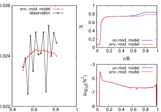
Figure 7: $\Delta P_{\mathrm{g}}$ pattern for the model obtained based on the non-standard modeling (red, denoted as “env.-mod. model”) and that for the observation (black). The model successfully reproduces the generally positive slope for periods smaller than $0.6\,d$ of the observed $\Delta P_{\mathrm{g}}$ pattern, but the other oscillatory component with a shorter period ($\Delta n\sim$ a few) cannot be reproduced with this model. Right panels show the internal structures (namely, the hydrogen profile in top panel and the $\rm{Brunt}$-$\rm{{V\ddot{a}is\ddot{a}l\ddot{a}}}$ frequency in bottom panel) of the envelope-modified model (red) and those of the corresponding unmodified model (blue, denoted as “un-mod. model”). We see two dips in the $\rm{Brunt}$-$\rm{{V\ddot{a}is\ddot{a}l\ddot{a}}}$ frequency of the envelope-modified model (bottom right), which are caused by the envelope modification implemented to the scheme of non-standard modeling. These features nevertheless do not affect the g-mode frequencies.

Figure 8: Comparison of the modeled frequencies (solid lines) with the observed ones (dashed lines) for the envelope-modified model obtained based on the non-standard modeling (bottom) and for the model of Kurtz et al. (2014). The radial, dipole, quadrupole, and octupole modes are represented by blue, red, green, and black, respectively. Note that the colors of the observed frequencies are based on the mode identification by Kurtz et al. (2014). In the case of the envelope-modified model, octupole modes are sometimes better to reproduce the observed frequencies than the dipole-mode frequencies of the model, implying the possibility of a different mode identification. See the text for more discussions.

Figure 8 shows the comparison of the modeled p-mode frequencies with the observed ones. The radial- (blue), dipole- (red), and quadrupole- (green) mode frequencies are presented. For our envelope-modified model, $l=3$ modes (black) are also illustrated. The envelope-modified model obtained in this study fits the observed radial-mode frequency better than the model of Kurtz et al. (2014). The other p-mode frequencies, however, are not fitted so well in the case of the envelope-modified model, especially when we follow the mode identification adopted in Kurtz et al. (2014) (see the caption of Figure 8 for more details). The mean deviation, which is defined as the mean of the absolute value of the difference between the modeled frequencies and the modeled ones, for our model is $0.2$ $d^{-1}$ while that of the best model in Kurtz et al. (2014) is $0.1$ $d^{-1}$.

However, we can at least claim that we have partly succeeded in constructing a comparable model with previous models; mean deviations of some of the previous models are sometimes larger than $0.5$ $d^{-1}$ (e.g. Takada-Hidai et al., 2017). We also would like to emphasize that the starting points are totally different for the current envelope-modified model and the previous models; in previous studies, we need to adopt too-high initial helium abundance of $\sim 0.3$–$0.4$ to explain the observed p-mode frequencies, but in this study, we can explain the observed ones with a much more ordinary initial helium abundance of $\sim 0.26$ by modeling the star in the non-standard manner where helium mass contents are suitably increased in the envelope.

Interestingly, when we include $l=3$ modes in the mode identification, the mean deviation for our model reduces to be $0.1$ $d^{-1}$ which is comparable to that of Kurtz et al. (2014). Although the mode identification of Kurtz et al. (2014) is reasonable in a sense that the spherical degree assigned to a certain mode is compatible with the number of the observed multiplets for the mode (if this is not the case, we need additional mechanisms to explain the reason why some modes in the multiplet are excited and the others are not), obtaining a hint for another possible way of mode identification for the star including $l=3$ modes could lead to further investigations that would, for example, challenge the theory of the mode excitation mechanism in $\delta$ Scuti stars, which has been definitely one of the unsettled subjects in asteroseismology.

5 Discussions

A few discussions about the non-standard model of the star are given in this section, namely, the evolutionary history (Section 5.1), the structure in the deep radiative region (Section 5.2), and a possible relation between the internal structure and dynamics (Section 5.3).

5.1 Single-star evolution or not?

One of the goals in this paper is to constrain the evolutionary history of KIC 11145123, which is here discussed from two different perspectives, namely, in terms of stellar modeling (this study) and in terms of abundance analyses (Takada-Hidai et al., 2017).

Though the envelope-modified models and the previous models are comparable with respect to the modeled frequencies (see discussions in Subsection 4.3.2), we would like to emphasize that the envelope-modified model is representing KIC 11145123 better. This is because we need not assume high initial helium abundance for the envelope-modified model. In contrast, it is difficult to explain the origin of the deduced high initial helium abundance of the previous models constructed assuming single-star evolution; we have to accept complex scenarios such as that the star was born in some high-helium environments, which is actually proposed for some globular clusters, though the cause of which has not been understood yet as well (Bastian and Lardo, 2018).

Then, if we persist to a single-star scenario for the star, the star should be a peculiar single star that has been kicked out of a globular cluster. Although it is possible that the star has been kicked out of a globular cluster judging from the kinematics of the star (Takada-Hidai et al., 2017), the chance that the star is the kind of peculiar single stars with high helium abundance is small because the sodium enrichment and the carbon depletion, both of which are always confirmed for the kind of stars (Bastian and Lardo, 2018), are not confirmed in the case of KIC 11145123 (Takada-Hidai et al., 2017). Combined with the fact that the abundance pattern of the star resembles those of typical blue straggler stars, it is probably the case that KIC 11145123 has experienced some interactions with other stars during the evolution.

Note that the envelope-modified model does not tell us about the corresponding progenitor because $\delta M=0$ in our envelope-modifying computations; there are in principle an infinite number of possible progenitors with different masses from which the envelope-modified model can be computed by “correctly” modifying the progenitors with the corresponding $\delta M$ (see the latter note on this issue in the beginning of Section 3). We nevertheless emphasize that what we originally would like to know was not the exact amount of mass gained by the star (via binary interactions or stellar merger) but whether the star could have experienced such envelope modification during the evolution or not, the latter of which can be achieved despite the fixed total mass $\delta M=0$.

One mystery remains to be solved; the star is currently not in a binary system (Takada-Hidai et al., 2017), and how the envelope of the star has been modified is still unknown. Since Takada-Hidai et al. (2017) have utilized the so-called phase modulation analysis (Murphy et al., 2016) to exclude the possibility of a binary system, they suggested that the star could belong to a binary whose spin-orbit is misaligned $90$ degrees (Murphy, 2018, private communication). Another possibility is that the star is a product of a more violent event such as stellar merger or stellar collision. This scenario naturally explains how the star has become a blue straggler star as well as the current rotational profile of the star that the envelope is rotating slightly faster than the deep radiative region (Kurtz et al., 2014), though it then challenges the origin of the very slow rotation of the star $P_{\mathrm{rot}}\sim 100\,\mathrm{d}$, i.e. a significant fraction of the angular momentum must have been lost from the star. Some numerical simulations have shown that the magnetic braking can contribute to the spin-down of collision products (e.g. Schneider et al., 2019). However, Takada-Hidai et al. (2017) have failed to detect the magnetic field ($>1\,\mathrm{kG}$) for the star, further complicating the discussion about the origin of the star. To reveal the exact cause of the envelope modification that the star has experienced is, as noted in the previous paragraph, beyond the scope in this paper, but that is definitely an interesting subject to investigate in the future.

5.2 G-mode period spacing ($\Delta P_{g}$) pattern revisited

The second discussion is about the structure in the deep radiative region of the star. We especially concentrate on the chemical composition gradient left behind the receding nuclear burning core, which sensitively affects $\Delta P_{\mathrm{g}}$ patterns (e.g. Miglio et al., 2008). After we show what impact steepness of chemical composition gradients has on the corresponding $\Delta P_{\mathrm{g}}$ patterns (Subsection 5.2.1), we propose a possible resolution for a deviation between the modeled $\Delta P_{\mathrm{g}}$ pattern and the observation based on a realistic stellar model (Subsection 5.2.2).

5.2.1 Chemical composition gradients vs $\Delta P_{\mathrm{g}}$ patterns

Figure 9: Numerically computed $\Delta P_{\mathrm{g}}$ patterns (colored curves) and the observed $\Delta P_{\mathrm{g}}$ pattern (black) are shown in the left panel. The corresponding internal structures, namely, the hydrogen profiles and the $\rm{Brunt}$-$\rm{{V\ddot{a}is\ddot{a}l\ddot{a}}}$ frequencies are illustrated in the right upper panel and the right lower panel, respectively. Note that the grey-shaded area in the lower right panel corresponds to the range of the abscissa for the upper right panel. The degree of perturbation (see equation (27) for one perturbation) becomes larger in the order of blue, green, and red, and correspondingly, an amplitude of an oscillatory component of a numerically computed $\Delta P_{\mathrm{g}}$ pattern becomes larger. We can confirm that the chemical composition gradient is successfully steepened with our scheme (see the hydrogen profiles or the $\rm{Brunt}$-$\rm{{V\ddot{a}is\ddot{a}l\ddot{a}}}$ frequencies at $r/R\sim 0.08$).

As demonstrated in Subsection 4.3.2, the envelope-modified model successfully reproduces the positive slope of the observed $\Delta P_{\mathrm{g}}$ pattern (Figure 7). Still, there is a discrepancy between the modeled $\Delta P_{\mathrm{g}}$ pattern (red in Figure 7) and the observed one (black in Figure 7) especially in terms of a short periodic component ($\Delta n\sim$ a few) seen in the observed $\Delta P_{\mathrm{g}}$ pattern.

It is generally considered that $\Delta P_{\mathrm{g}}$ patterns can be analytically described as oscillating components (in terms of the g-mode radial order) whose periods and amplitudes are determined by locations and strengths, respectively, of the sharp features in the chemical composition gradients (more precisely, the sharp features in the $\rm{Brunt}$-$\rm{{V\ddot{a}is\ddot{a}l\ddot{a}}}$ frequencies, see more discussions in, e.g., Miglio et al., 2008).

Thus, one possible approach to reproduce the shorter-period component of the observed $\Delta P_{\mathrm{g}}$ pattern is to add artificial perturbations in the chemical composition gradients and to render the gradients be steeper, which can be achieved by applying the scheme of constructing stellar models whose chemical compositions are arbitrarily modified (demonstrated in Section 3).

Then, which part of the chemical composition gradient should we perturb? The period of the oscillatory component in the $\Delta P_{\mathrm{g}}$ pattern, in particular, is determined by the ratio $\Pi_{\mu}/\Pi_{0}$, where

$$\Pi_{0}^{-1}=\int_{r_{0}}^{r_{1}}Nd\,\mathrm{ln}\,r,$$ (25)

and

$$\Pi_{\mu}^{-1}=\int_{r_{0}}^{r_{\mu}}Nd\,\mathrm{ln}\,r$$ (26)

(Miglio et al., 2008). The $\rm{Brunt}$-$\rm{{V\ddot{a}is\ddot{a}l\ddot{a}}}$ frequency is denoted by $N$. The inner edge of the (high-order) g-mode cavity, the outer one, and the location of the sharp feature in $N$ are $r_{0}$, $r_{1}$, and $r_{\mu}$, respectively. We thus perturb the outer region of the chemical composition gradient (see around $r/R\sim 0.08$ in Figure 9) with which the ratio $\Pi_{\mu}/\Pi_{0}\sim 3$, close to the short period ($\Delta n\sim$ a few) in the observed $\Delta P_{\mathrm{g}}$ pattern.

Figure 9 illustrates $\Delta P_{\mathrm{g}}$ patterns which are numerically computed based on the perturbed models obtained using the resettling function; they are in both hydrostatic and thermal equilibrium states. In order to obtain the perturbed models, we perturb the deep radiative region, instead of the envelope as in Section 4, so that the chemical composition gradient becomes steeper, using the following expression for one perturbation:

$$\delta X\equiv B_{\mathrm{G}}\times\mathrm{exp}\biggl{[}-\frac{1}{2}\biggl{(}\frac{m-m_{\mathrm{c}}}{A_{\mathrm{G}}}\biggr{)}^{2}\biggr{]},$$ (27)

where $B_{\mathrm{G}}$, $m_{\mathrm{c}}$, and $A_{\mathrm{G}}$ are the amplitude, the center, and the width of the modification, respectively. The specific values are as follows: $B_{\mathrm{G}}=5\times 10^{-4}$, $m_{\mathrm{c}}=0.2826$, and $A_{\mathrm{G}}=10^{-2}$. Then, the deviated models are resettled to hydrostatic states with our scheme (see details in Section 3).

It is clearly seen that our scheme successfully provides us with the equilibrium stellar models with the chemical composition gradients much steeper than that of the unperturbed model. It is also verified that an amplitude of the shorter-period component of a numerically computed $\Delta P_{\mathrm{g}}$ pattern becomes larger as the model is perturbed more (from blue to red in Figure 9), which is the same trend as expected by Miglio et al. (2008).

5.2.2 Realizing steeper chemical composition gradients with a more realistic stellar model

Figure 10: Observed g-mode period spacings $\Delta P_{\rm{g}}$ (black thick line) and modeled g-mode period spacings (the red line and the blue line) in the left panel. The red line is calculated based on the envelope-modified model (here, denoted as “o.-diff. model”, short for “ordinary-diffusion model”), and the blue line is based on another model with weaker elemental diffusion (here, denoted as “w.-diff. model”, short for “weaker-diffusion model”). The latter model successfully reproduces the period of the short-periodic oscillatory component of the observed $\Delta P_{\rm{g}}$ pattern. We also see some improvements in terms of the amplitude of the short-periodic oscillatory component of $\Delta P_{\rm{g}}$ pattern compared with that of the envelope-modified model. The right panels show the corresponding hydrogen profiles (top) and $\rm{Brunt}$-$\rm{{V\ddot{a}is\ddot{a}l\ddot{a}}}$ frequencies (bottom). It is obvious that the chemical composition gradient of the weaker-diffusion model is much steeper than that of the envelope-modified model.

In the previous subsection, it has been suggested that to consider an artificial perturbation to the chemical composition gradient could be helpful for reproducing the short-periodic component based on the direct numerical computations of the eigenfrequencies for several perturbed chemical composition gradients. In particular, perturbing chemical composition gradients so that the gradients become steeper is a possible solution to reproduce the shorter-period component of the observed $\Delta P_{\mathrm{g}}$ pattern. Then, the next question is what is the mechanism that is at work during the evolution and produces such structures?

One of the straightforward ways to produce such steep chemical composition gradients is not to activate elemental diffusion in 1-d stellar evolutionary calculations; the diffusion process renders the chemical composition gradient less steep. Still, elemental diffusion is generally expected to be at work inside stars (Michaud et al., 2015), and thus, in this subsection, we consider a model with elemental diffusion, but “much weaker” diffusion processes during evolution.

We implement such “much weaker” diffusion by changing the default criterion for the maximum diffusion velocity ($\mathrm{diffusion}\_\mathrm{v}\_\mathrm{max}$ $=$ $1.$d$-$3 adopted in MESA) to a much smaller value ($\mathrm{diffusion}\_\mathrm{v}\_\mathrm{max}$ $=$ $1.$d$-$10). Specifically, we force the gravitational settling to be suppressed (note that we do not include radiative levitation in our computations as described in Section 2).

In MESA, the diffusion velocity of each element in each mass shell is computed by solving Burgers’ equation (Burgers, 1969), which sometimes leads to unphysically large diffusion velocities in, for instance, the outermost envelope. The criterion $\mathrm{diffusion}\_\mathrm{v}\_\mathrm{max}$ in MESA is thus usually set to avoid such problems, and our implementation is rather crude in a sense that our purpose of setting $\mathrm{diffusion}\_\mathrm{v}\_\mathrm{max}$ is different from the original one as Paxton et al. (2011) have proposed. Nevertheless, we clearly see improvements in the behavior of a short periodic component in the $\Delta P_{\mathrm{g}}$ pattern computed with the much weaker diffusion processes during evolution (see Figure 10), showing a high potential of the implementation for further asteroseismic researches.

It should be noted, however, that the implementation is computationally fairly time-consuming, and that it is still hard to incorporate the scheme into, for example, the grid-based modeling of stars. This is due to the presence of discontinuities in chemical composition gradients caused by the weaker diffusion, leading to very small timesteps in stellar evolutionary computations (see more details in Paxton et al., 2011).

Another point worth mentioning is that radiative levitation, which has been phenomenologically treated with the scheme of Morel and Thevenin (2002) in this study, can counteract the gravitational settling to reduce net velocities for elemental diffusion as shown by Deal et al. (2018), and thus, including radiative levitation in computations of elemental diffusion could be a promising next step to be done in the near future.

5.3 A relation between the inferred steeper $\nabla_{\mu}$ and the fast-core rotation?

In the previous subsection, we see that adopting “much weaker” diffusion in our computations partly successfully reproduces the observed $\Delta P_{\mathrm{g}}$ pattern. But we cannot immediately conclude that the diffusion process inside the star is really weak since mixing processes other than convection, convective overshoot, and diffusion are neglected in our 1-d stellar evolutionary computations, among which rotation is known to cause extra mixing processes inside stars as well as to counteract diffusion processes (e.g. Deal et al., 2020).

Interestingly, Hatta et al. (2019) have pointed out the possibility that the convective core of KIC 11145123 is rotating 5–6 times faster than the other regions of the star. Therefore, for KIC 11145123, it is expected that the inferred fast-core rotation, or the inferred rotational velocity shear between the convective core and the radiative region above, can cause instabilities which lead to mixing around the convective core boundary.

Then, let us focus on such extra mixing caused by rotational shear instabilities. We have the following two possibilities regarding the inferred steeper chemical composition gradient of the star. The first possibility is that diffusion process is really weak (more precisely, somehow much weaker than the current theoretical computations predict) and the rotationally induced mixing can be ignored (though the rotational velocity shear does exist), leading to the inferred chemical composition gradient. Or, the second possibility is that the diffusion is working as the theory predicts but the rotationally induced mixing effectively counteracts the diffusion, leading to the inferred chemical composition gradient.

Actually, a relation, similar to that suggested by the second possibility, between internal dynamics and structure can be also found in the case of the Sun. According to results of helioseismic structure inversion, there is a discrepancy between the sound speed profile of the real Sun and that of the standard solar model at the bottom of the solar convective envelope (Christensen-Dalsgaard et al., 1996). Interestingly, the bottom of the convective envelope where the discrepancy has been found is close to the so-called solar tachochline, a relatively strong rotational velocity shear inferred based on helioseismic rotation inversion (Thompson et al., 1996), and it is currently commonly accepted in the helioseismology community that the discrepancy can be resolved if we consider extra mixing caused by the velocity shear at the solar tachochline. (See more detailed discussions in, e.g., Gough et al., 1996; Christensen-Dalsgaard, 2021).

The second possibility that the rotation-induced mixing counteracts the elemental diffusion thus seems to be more attractive compared with the first possibility that the elemental diffusion is really weak. But here is one caveat; in helioseismology, extra mixings at the solar tachochline are believed to mix the region uniformly (reducing effectiveness of the helium gravitational settling), but in the case of KIC 11145123, we have an opposite trend where extra mixings around the convective boundary render the chemical composition gradient to be steeper somewhere. The latter process might sound peculiar for us because mixing processes, literally, mix the chemical composition uniformly. However, whether a mixing process really leads to a locally uniform chemical composition profile or not strongly depends on the scaleheight of the mixing process and the position where the mixing is at work; if the mixing region is too thin and the mixing is occurring at the edge of the boundary (in terms of the chemical composition profile, for instance), the gradient of the chemical composition profile can be maintained, or even strengthen, though the chemical composition is uniform inside the thin mixing region, which might be the case for KIC 11145123.

Figure 11: Numerically computed $\Delta P_{\mathrm{g}}$ patterns (left), hydrogen mass contents (upper right), and $\rm{Brunt}$-$\rm{{V\ddot{a}is\ddot{a}l\ddot{a}}}$ frequencies (lower right) of models whose chemical composition gradients are modified. The modifications are given mimicking extra mixings caused by rotational shear instabilities around the convective boundary, leading to chemically uniform regions such as those seen between $0.065<r/R<0.07$ (see the upper right panel). Note that the chemical compositions in the modified region are not exactly the same as those in the convective core due to the thermally-evolving step in the resettling scheme (see the last paragraph of Section 3.1). It is seen that as we render the fully mixed region broader (from light blue to red), the dip in the $\Delta P_{\mathrm{g}}$ patterns become larger (see also light blue curves to red curves). The numerically computed $\Delta P_{\mathrm{g}}$ patterns nevertheless do not reproduce a shorter-period component as that confirmed in the observed $\Delta P_{\mathrm{g}}$ pattern (black). The grey-shaded area in the lower right panel corresponds to the range of the abscissa for the upper right panel, as in Figure 9.

To test the possibilities, we again utilize the resettling function to obtain stellar models whose chemical composition gradients are modified, as demonstrated in Subsection 5.2.1. In this case, we have mimicked the extra mixing originating from rotational shear instabilities by artificially rendering the chemical composition gradients developed just above the convective core to be uniform; in the modified region, the chemical compositions are homogeneous and almost the same as those in the convective core (Figure 11). Once we resettle the perturbed model to the hydrostatic and thermal equilibrium state, we have extended the uniformly modified region by $6\times 10^{-4}$ in fractional radius per one modification, and repeated the process described above until the upper boundary of the artificially well-mixed region reaches $r/R\sim 0.068$ (which corresponds to the red curves in Figure 11).

Figure 11 shows structures of thus obtained models (right panels) and the corresponding $\Delta P_{\mathrm{g}}$ patterns (left panel). It is clearly seen that the chemical composition gradients can be locally steeper in the presence of the relatively small-scale mixing, which has been expected from the discussions in the preceding paragraphs. However, we do not see any improvements in the numerically computed $\Delta P_{\mathrm{g}}$ patterns; the observed short-period oscillatory component is not reproduced by any modified models. This is because, in this case, the ratio $\Pi_{\mu}/\Pi_{0}$ (see the expressions 25 and 26) is much larger than $3$, which is expected to reproduce the shorter periodic component in the observed $\Delta P_{\mathrm{g}}$ pattern, resulting in a longer periodic component in the numerically computed $\Delta P_{\mathrm{g}}$ patterns (see discussions in Section 5.2). We therefore cannot explain the observed $\Delta P_{\mathrm{g}}$ pattern based on the assumption that the rotationally induced mixing is counteracting the elemental diffusion process, and we consider the first possibility, that the diffusion process is somehow really weak in the deep region of the star, more probable compared with the other possibility.

6 Conclusions

This paper is dedicated to detailed asteroseismic non-standard modeling of a possible blue straggler star, KIC 11145123. Two main conclusions have been obtained and they are listed in the following paragraphs.

The first conclusion is that the star might have been born as a single star with an ordinary initial helium abundance of $\sim 0.26$ and then experienced some interactions with other stars, leading to the modification of the chemical composition in the envelope. This conclusion is obtained based on the non-standard asteroseismic modeling of the star where modifications of the chemical compositions are taken into account for constructing 1-dimensional stellar models. A scheme to compute such non-standard models has been developed in this study, which is applied to the comprehensive grid-based modeling of the star, resulting in the envelope-modified model with fundamental parameters as below: $M=1.36M_{\odot}$, $Y_{\mathrm{init}}=0.26$, $Z_{\mathrm{init}}=0.002$, and $f_{\mathrm{ovs}}=0.027$. The modification is down to the depth of $r/R\sim 0.6$ and the extent is $\Delta X\sim 0.06$ ($\Delta X$ is the difference in hydrogen abundance between the unmodified model and the modified model) at the surface. This is the first time such an envelope-modified model (which is still in both hydrostatic and thermal equilibrium states) is obtained for the star, and the discrepancy between the modeled eigenfrequencies and the observed ones is comparable to those for previous models computed based on an assumption of a single-star evolution and high initial helium abundance. The conclusion that this star may well have experienced some interactions with other stars during the evolution is consistent with the formation channels of blue straggler stars, thus strengthening the argument that the star is a (probable rather than possible) blue straggler star.

The second conclusion is that the elemental diffusion in the deep region of the star might be much weaker than that assumed in ordinary stellar evolutionary calculations. This conclusion is obtained based on the detailed analysis of the observed $\Delta P_{\mathrm{g}}$ pattern of the star, which evidently suggests that the chemical composition gradient in the deep radiative region above the convective core should be much steeper than that of the envelope-modified model. Though exact mechanisms to render the chemical composition gradient so steep are not clear yet, this is the first study which tests the possibility that there is a relationship between the current rotational profile and the structure of the stars, and to investigate such relationship should be one of the most highly prioritized subjects to future researches.

References

- Aerts et al. (2010) Aerts, C., Christensen-Dalsgaard, J., Kurtz, D. W. 2010, AA Library, “Asteroseismology”
- Aerts et al. (2017) Aerts, C., Van Reeth, T., Tkachenko, A. 2017, ApJL, 847, L7
- Aerts et al. (2019) Aerts, C., Mathis, S., Rogers, T. M. 2019, Annu. Rev. Astron. Astrophys., 57, 35
- Bastian and Lardo (2018) Bastian, N. Lardo, C. 2018, Annu. Rev. Astron. Astrophys., 56, 83
- Bedding et al. (2011) Bedding, T. R., Mosser, B., Huber, D., et al., 2011, Nature Letters, VOL 471, p. 608-611
- Boffin et al. (2015) Boffin, M. J., et al. 2015, Astrophysics and Space Science Library, 413
- Brogaard et al. (2018) Brogaard, K., Christiansen. S. M., Grundahl, F., et al. 2018, MNRAS, 481, 5062-5072
- Burgers (1969) Burgers, J. M. 1969, Flow Equations for Composite Gases (New York: Academic)
- Chaplin and Miglio (2013) Chaplin, W. J. Miglio, A. 2013, Annu. Rev. Astron. Astrophys., 51: 353-392
- Christensen-Dalsgaard et al. (1996) Christensen-Dalsgaard, J., Däppen, W., Ajukov, S. V., et al. 1996, Science, Volume 272, Issue 5266, pp. 1284-1286
- Christensen-Dalsgaard (2021) Christensen-Dalsgaard, J. 2021, Living Reviews in Solar Physics, Volume 18, Issue 1, article id.2
- Deal et al. (2018) Deal, M., Alecian, G., Lebreton, Y., et al. 2018, AA, 618, 10
- Deal et al. (2020) Deal, M., Goupil, M.-J., Marques, J. P., et al. 2020, AA, 633, 23
- Gizon et al. (2016) Gizon, L., Sekii, T., Takata, M., et al. 2016, Science Advances, 2: e1601777
- Gough et al. (1996) Gough, D. O., Kosovichev, A. G., Toomre, J., et al. 1996, Science, Volume 272, Issue 5266, pp. 1296-1300
- Hatta et al. (2019) Hatta, Y., Sekii, T., Takata, M., Kurtz, D. W. 2019, ApJ, 871, 135
- Herwig (2000) Herwig, F. 2000, AA, 360, 952
- Huber et al. (2014) Huber, D., Silva Aguirre, V., Matthews, J. M., et al. 2014, ApJS, 211, 2
- Kippenhahn et al. (2012) Kippenhahn, R., Weigert, A., Weiss, A. 2012, AA Library
- Koch et al. (2010) Koch, D. G., Borucki, W. J., Basri, G., et al. 2010, ApJL, 713, L79
- Kosovichev and Kitiashvili (2020) Kosovichev, A. G. Kitiashvili, I. N. 2020, IAUS, 354, 107
- Kurtz et al. (2014) Kurtz, D. W., Saio, H., Takata, M. et al. 2014, MNRAS, 444, 102
- Michaud et al. (2015) Michaud, G., Alecian, G., Richer, J. 2015, AA Library, “Atomic Diffusion in Stars”
- Miglio et al. (2008) Miglio, A., Montalban, J., Noels, A., Eggenberger, P. 2008, MNRAS, 386, 1487-1502
- Morel and Thevenin (2002) Morel, P. Thevenin, F. 2002, AA 390, 611-620
- Murphy et al. (2016) Murphy, S. J., Bedding, T. R., Shibahashi, H. 2016, ApJ Letters, 827: L17 (4pp)
- Paxton et al. (2011) Paxton, B., Bildsten, L., Dotter, A., et al. 2011, ApJ Supplement Series, 192, 3
- Paxton et al. (2013) Paxton, B., Cantiello, M., Arras, P., et al. 2013, ApJ Supplement Series, 208, 4
- Paxton et al. (2015) Paxton, B., Marchant, P., Schwab, J., et al. 2015, ApJ Supplement Series, 220, 15
- Paxton et al. (2018) Paxton, B., Schwab, J., Bauer, E. B., et al. 2018, ApJ Supplement Series, 234, 34
- Paxton et al. (2019) Paxton, B., Smolec, R., Schwab, J., et al. 2019, ApJ Supplement Series, 243, 10
- Ricker et al. (2014) Ricker, G. R., Winn, J. N., Vanderspek, R., et al. 2014, SPIE, 9143, 20
- Saio et al. (2015) Saio, H., Kurtz, D. W., Takata, M., et al. 2015, MNRAS 447, 3264
- Sandage (1953) Sandage, A. R. 1953, Astronomical Journal, 58, 61
- Schmid and Aerts (2016) Schmid, V. S., Aerts, C. 2016, AA, 592, A116
- Schneider et al. (2019) Schneider, F. R. N., Ohlman, S. T., Podsiadlowski, P., et al. 2019, Nature, 574, 211
- Takada-Hidai et al. (2017) Takada-Hidai, M., Kurtz, D. W., Shibahashi, H. et al. 2017, MNRAS, 470, 4908-4924
- Thompson et al. (1996) Thompson, M. J., Toomre, J., Anderson, E. R., et al. 1996, Sci, 272, 1300
- Townsend and Teitler (2013) Townsend, R. H. D. Teitler, A. 2013, MNRAS 435, 3406-3418
- Unno et al. (1989) Unno, W., Osaki, Y., Ando, H., Saio, H., Shibahashi, H. 1989, Univ. Tokyo Press, “Nonradial Oscillations of Stars”