Large time and long distance asymptotics of the thermal correlators
of the impenetrable anyonic lattice gas

Abstract

We study thermal correlation functions of the one-dimensional impenetrable lattice anyons. These correlation functions can be presented as a difference of two Fredholm determinants. To describe large time and long distance behavior of these objects we use the effective form factor approach. The asymptotic behavior is different in the space-like and time-like regions. In particular, in the time-like region we observe the additional power factor on top of the exponential decay. We argue that this result is universal as it is related to the discontinuous behavior of the phase shift function of the effective fermions. At particular values of the anyonic parameter, we recover asymptotics of spin-spin correlation functions in XXO quantum chain.

I Introduction

Quantum one-dimensional models always attracted a lot of attention due to rich structures of their correlation functions and the possibility to address non-perturbative phenomena [1, 2, 3]. For low temperatures the culmination of these developments resulted in the formulation of effective fields theories (Luttinger model) [3, 4]. With the advancement of the experimental techniques in cold atom experiments [5, 6, 7, 8] the interest to the non-equilibrium dynamics or dynamics of highly excited states motivated a lot of theoretical research resulting in new concepts like generalized Gibbs ensembles, the quench action [9, 10], the generalized hydrodynamics [11, 12, 13] (GHD) and others. The main approach to the correlation function in integrable models is a direct summation of the form factors in the spectral expansion. The computation of the correlation functions on the finite entropy states is very different from the vacuum case due to different decay rate of the form factors with the system size (exponential vs power-law). Therefore, different approaches were developed to tackle this kind of problems including Quantum Transfer Matrix approach [14, 15, 16, 17, 18, 19, 20], non-linear differential equations [21, 22], axiomatic definition of the thermal form factors in the Integrable Quantum Field Theories [23, 24, 25, 26, 27, 28, 29, 30, 31], adaptation of the GHD methods [32, 33, 34, 35], as well as partial summations of the few particle-hole excitations [36, 37, 38, 39, 40] and extracting the most singular parts of the form factors [41, 42].

Recently we have developed a method to deal with correlation functions in finite entropy states [43]. This method allows one to derive behaviour of the correlation functions in free-fermionic models for the observables that can be expressed as Fredholm determinants of integrable kernels. In Ref. [43] we focused mostly on static correlation functions and have applied the method to XY quantum chain.

In this work we continue development of the method of effective form factors for dynamical correlation functions. As a model of interest we choose one-dimensional impenetrable anyons on a lattice [44]. This model describes quantum particles with unusual statistics [45, 46, 47, 48, 44, 49], which can be realized experimentally in ultracold quantum gases confined in optical traps [50, 51, 52, 53, 54, 55, 56, 57, 58]. Furthermore, this type of models appears after the spin-charge separation in interacting systems of spinful fermions and spin chains (at certain values of the anyonic parameter) [59, 60, 61, 62, 63, 64, 65, 66, 67]. Similar determinants also can be obtained as the correlation functions of Wigner strings [68]. Also they appear in the describing the mobile impurity propagating in the gas of free fermions [69, 70, 71, 72]. In the latter case the anyonic parameter can be identified with the total momentum of the system (at the infinite coupling).

The main idea of the effective form factor approach is to replace computation of the correlation functions averaged over some ensemble to zero temperature correlators with the appropriately modified phase shift. The correlation functions for one-dimensional impenetrable anyons can be presented as a linear combination of the Fredholm determinants [44]. Therefore we may identify the phase shift comparing these determinants to the one that emerges from the summation of the effective form factors. For the space-like region we can simplify the corresponding kernels for large time and space separation and find the effective phase shift for all values of the quasi momenta. The time-like region is characterized by the critical points that separate different types of the asymptotic behavior. So we can robustly find the effective phase shift only away from these points. Even though the vicinity of critical points where we do not know the solutions vanish in the large time limit, we cannot simply combine solutions in the different asymptotic regions into a single phase shift as the latter will be discontinuous. To tackle this problem we have assumed the existence of the gluing regularization functions. While we have not been able to find them explicitly, we have demonstrated that they only affect the overall constant in the asymptotic expression of the Fredholm determinants.

The structure of the paper is as follows. In Sec. II we define the anyonic model and review important results about this model, such as spectrum and presentation of correlation functions in terms of Fredholm determinants. In Sec. III we recall the effective form factor approach and give two expressions for the $\tau$ function in the thermodynamic limit. In Sec. IV the effective form factor approach is applied to the derivation of the large time and long distance asymptotics of the dynamical correlation functions. We discuss separately space-like and time-like regimes. In Sec. V we summarize the main results of the paper, compare with the known results in literature and discuss different possibilities for further research. Appendix contains technical details of the asymptotic analysis of the form factors with the regularized effective phase shift.

II Model

The one-dimensional impenetrable lattice anyons on $L$ sites can be described by the following Hamiltonian [44]

$$H=-\sum_{j=1}^{L}\frac{1}{2}(a^{{\dagger}}_{j}a_{j+1}+a^{{\dagger}}_{j+1}a_{j})+h\sum_{j=1}^{L}a^{{\dagger}}_{j}a_{j},$$ (1)

$$a_{L+1}=a_{1},\qquad a^{{\dagger}}_{L+1}=a^{{\dagger}}_{1}.$$ (2)

The operator algebra is specified by the anyonic parameter $0\leq\kappa\leq 1$ and reads as

$$a_{j}a^{{\dagger}}_{k}=\delta_{jk}-e^{-i\pi\kappa\epsilon(j-k)}a^{{\dagger}}_{k}a_{j},$$ (3a)

$$a_{j}a_{k}=-e^{i\pi\kappa\epsilon(j-k)}a_{k}a_{j},$$ (3b)

$$a^{{\dagger}}_{j}a^{{\dagger}}_{k}=-e^{i\pi\kappa\epsilon(j-k)}a^{{\dagger}}_{k}a^{{\dagger}}_{j},$$ (3c)

here $\epsilon(j)=\mathrm{sign}(j)$ and we prescribe that $\epsilon(0)=0$.

The case $\kappa=0$ corresponds to fermions, and $\kappa=1$ describes operators in the Hilbert space of the impenetrable bosons. Note, also that in the latter case the Hamiltonian (1) can be identified with the Hamiltonian of quantum XX spin chain after the mapping $a_{j}=\sigma_{j}^{+}$, $a_{j}^{\dagger}=\sigma_{j}^{-}$.

Spectrum of the Hamiltonian $H$ can be found by means of Bethe ansatz. The $N$-particle states are labeled by $N$ momenta $\{p_{1},p_{2},\ldots,p_{N}\}$ from the set of $L$ inequivalent solutions of the equation

$$e^{ipL}=e^{-i\pi\kappa(N-1)}.$$ (4)

The energies of such states are

$$E(\{p_{1},p_{2},\ldots,p_{N}\})=\sum_{j=1}^{N}\varepsilon(p_{j}),$$ (5)

$$\varepsilon(p)=h-\cos p.$$ (6)

An interesting and non-trivial problem in the considered model is to analyze two-point correlation functions

$$G_{-}(x,t)=\frac{\mathrm{Tr}[e^{-\beta H}a^{{\dagger}}_{x+1}(t)a_{1}(0)]}{\mathrm{Tr}[e^{-\beta H}]},$$ (7)

$$G_{+}(x,t)=\frac{\mathrm{Tr}[e^{-\beta H}a_{x+1}(t)a^{{\dagger}}_{1}(0)]}{\mathrm{Tr}[e^{-\beta H}]}.$$ (8)

It is easy to check the symmetry relations

$$G_{\pm}(-x,-t)=G_{\pm}(x,t)^{*},$$ (9)

and also for $t=0$

$$G_{-}(x,0)+e^{-i\pi\kappa\,\mathrm{sign}(x)}G_{+}(-x,0)=\delta_{x,0}$$ (10)

which allow us to consider only $t\geq 0$. In what follows we will restrict ourselves to the analysis of correlator $G_{-}(x,t)$. An analogous analysis can be done for $G_{+}(x,t)$. It was shown that these correlators in the thermodynamic limit $L\to\infty$ can be written in terms of Fredholm determinants [44]. We will use the following equivalent presentation for $G_{-}(x,t)$:

$$G_{-}(x,t)=\det(1+\hat{W}+\delta\hat{W})-\det(1+\hat{W}),$$ (11)

where $\hat{W}$ and $\delta\hat{W}$ are integral operators on $[-\pi,\pi]$ with the kernels

$$W(p,q)=\frac{1}{2\pi}e_{-}(p)e_{-}(q)e^{\frac{i(p-q)}{2}}\frac{e(p)-e(q)}{\sin\frac{p-q}{2}},$$ (12)

$$\delta W(p,q)=\frac{1}{2\pi}e_{-}(p)e_{-}(q),$$ (13)

$$n_{F}(p)=\frac{1}{e^{\beta\varepsilon(p)}+1},$$ (14)

$$e_{-}(p)=\sqrt{n_{F}(p)}e^{-ixp/2+it\varepsilon(p)/2},$$ (15)

$$e(p)=\sin^{2}\frac{\pi\kappa}{2}\fint_{-\pi}^{\pi}\frac{dq}{2\pi}e^{ixq-it\varepsilon(q)}\cot\frac{q-p}{2}\\ +\frac{1}{2}\sin(\pi\kappa)e^{ixp-it\varepsilon(p)}.$$ (16)

Eq. (11) allows us to compute the correlation function $G_{-}(x,t)$ numerically. However, large time and long distance asymptotics of the correlation functions are hard to extract by numerical means due to the oscillatory behavior of integral kernels. In the present paper we instead analyze these asymptotics analytically by means of the effective form factor approach [43], which is briefly reviewed below.

III Effective form factor approach

III.1 Effective form factors and tau function

In this section we recall the effective form factor approach initiated in [43]. To specify the effective form factor we require two smooth periodic functions $\nu(k)$, $g(k)$. The first one is called the effective phase shift and defines the shifted set of momenta as solutions of

$$e^{ikL}=e^{-2\pi i\nu(k)}.$$ (17)

Here $L$ is regarded as a system size. Since $\nu(k)$ is periodic, i.e. has a zero winding number in term of [43], the largest ordered set of the shifted momenta has $L$ terms $\mathbf{k}=\{k_{1},\ldots,k_{L}\}$. Each $k_{i}$ is a solution of (17). The unshifted momenta are solutions of

$$e^{iqL}=1.$$ (18)

All momenta are considered up to the equivalence ${k\sim k+2\pi}$ and it is convenient to choose them to have real parts in the Brillouin zone $[-\pi,\pi]$.

The effective form factors are defined for the subsets of momenta $\mathbf{q}$ of the size $L-1$. Such subsets can be parameterized by the position of the “hole”

$$\mathbf{q}^{(a)}=\{q_{1},\ldots,q_{a-1},q_{a+1},\ldots,q_{L}\},\quad a=1,\ldots,L.$$ (19)

The effective form factor then reads

$$|\langle\textbf{k}|\mathbf{q}^{(a)}\rangle|^{2}=L^{1-2L}\prod_{j=1}^{L}\frac{e^{g(k_{j})-g(q_{j})}\sin^{2}\pi\nu(k_{j})}{1+\frac{2\pi}{L}\nu^{\prime}(k_{j})}\\ \times e^{g(q_{a})}{\det}^{2}D^{a},$$ (20)

where ${\det}D^{a}$ is defined for $\mathbf{q}^{(a)}$ and is nothing but a trigonometric variation of the Cauchy determinant, in which the row corresponding to $q_{a}$ is omitted and replaced with the line of $1$

$${\det}D^{a}=\begin{vmatrix}\cot\frac{k_{1}-q_{1}}{2}&\dots&\cot\frac{k_{L}-q_{1}}{2}\\ \vdots&\ddots&\vdots\\ \cot\frac{k_{1}-q_{L}}{2}&\dots&\cot\frac{k_{L}-q_{L}}{2}\\ 1&\dots&1\\ \end{vmatrix},$$ (21)

as we deal only with the square of the determinant we can put this line to be the last one.

The tau (correlation) function is defined as series over these form factors

$$\tau(x,t)=\sum_{{\bf q}^{a}}|\langle{\bf k}|{\bf q}^{a}\rangle|^{2}e^{-ix(P({\bf k})-P({\bf q}^{a}))+it(E({\bf k})-E({\bf q}^{a}))}.$$ (22)

Here we use notations for the momentum and energy of many-particle state $|{\bf q}\rangle$

$$P({\bf q})=\sum_{q\in{\bf q}}q,\quad E({\bf q})=\sum_{q\in{\bf q}}\varepsilon(q).$$ (23)

In Ref. [43] we have demonstrated that in the thermodynamic limit $L\to\infty$ the tau function can be presented as a difference of two Fredholm determinants

$$\tau(x,t)=\det(1+\hat{V}+\delta\hat{V})-\det(1+\hat{V}),$$ (24)

where $\hat{V}$ and $\delta\hat{V}$ are integral operators on $[-\pi,\pi]$ with kernels

$$V(p,q)=\frac{1}{2\pi}c_{-}(p)c_{-}(q)e^{\frac{i(p-q)}{2}}\frac{c(p)-c(q)}{\sin\frac{p-q}{2}},$$ (25)

$$\delta V(p,q)=\frac{1}{2\pi}c_{-}(p)c_{-}(q),$$ (26)

$$c_{-}(p)=\sin\pi\nu(p)e^{-ixp/2+it\varepsilon(p)/2+g(p)/2},$$ (27)

$$c(p)=\fint_{-\pi}^{\pi}\frac{dq}{2\pi}e^{ixq-it\varepsilon(q)-g(q)}\cot\frac{q-p}{2}\\ +\cot\pi\nu(p)e^{ixp-it\varepsilon(p)-g(p)}.$$ (28)

This form allows us to relate the correlation function of anyons with the tau function for a special choice of $\nu(k)$ and $g(k)$. This relation will be described in the next section.

III.2 Finite size scaling

In this subsection we give an alternative formula for the tau function based on the first taking the thermodynamic limit of the form factors and then performing the summation. The obtained expressions will have a simple form convenient for asymptotic analysis [43].

We start from representing ${\det}D^{a}$ in a factorized form

$$\prod_{i=1}^{L}\frac{\sin^{2}\pi\nu(k_{i})}{L^{2}}{\det}^{2}D^{(a)}=Z^{2}\mathcal{Z}_{a},$$ (29)

$$Z=\prod\limits_{i=1}^{L}\prod\limits_{j=1}^{i-1}\frac{\sin\frac{k_{i}-k_{j}}{2}}{\sin\frac{q_{i}-q_{j}}{2}},$$ (30)

$$\mathcal{Z}_{a}=\sin^{2}\frac{\pi\nu(k_{a})}{L}\prod\limits_{j\neq a}^{L}\frac{\sin^{2}\frac{k_{j}-q_{a}}{2}}{\sin^{2}\frac{q_{j}-q_{a}}{2}}.$$ (31)

Extracting the hole dependent factors the tau function (22) can be rewritten as

$$\tau(x,t)=L\cdot K(x,t)\cdot\sum\limits_{a=1}^{L}e^{g(q_{a})}\mathcal{Z}_{a}e^{-ixq_{a}+it\varepsilon(q_{a})},$$ (32)

where $K(x,t)$ is $a$-independent part given by

$$K(x,t)=Z^{2}e^{-ix(P({\bf k})-P({\bf q}))+it(E({\bf k})-E({\bf q}))}\\ \times\prod_{j=1}^{L}\frac{e^{g(k_{j})-g(q_{j})}}{1+\frac{2\pi}{L}\nu^{\prime}(k_{j})}.$$ (33)

The expressions $Z^{2}$ and $K(x,t)$ have finite thermodynamic limit [43]

$$\log Z=-\int\limits_{-\pi}^{\pi}dq\int\limits_{-\pi}^{\pi}dk\left[\frac{\nu(q)-\nu(k)}{4\sin\frac{q-k}{2}}\right]^{2},$$ (34)

$$\log K(x,t)=2\log Z-\int\limits_{-\pi}^{\pi}\nu(q)g^{\prime}(q)dq\\ +i\int\limits_{-\pi}^{\pi}(x-\varepsilon^{\prime}(q)t)\nu(q)dq.$$ (35)

The hole dependent factors are suppressed in the thermodynamic limit

$$\mathcal{Z}_{a}\approx L^{-2}\sin^{2}\pi\nu(q_{a})\exp\left(-\fint\limits_{-\pi}^{\pi}dq\,\nu(q)\cot\frac{q-q_{a}}{2}\right),$$ (36)

but the whole tau function (32) has finite thermodynamic limit and can be presented as an integral

$$\tau(x,t)=K(x,t)\int\limits_{-\pi}^{\pi}\frac{dk}{2\pi}e^{g(k)}\sin^{2}\pi\nu(k)e^{-ixk+it\varepsilon(k)}\\ \times\exp\left(-\fint\limits_{-\pi}^{\pi}dq\,\nu(q)\cot\frac{q-k}{2}\right).$$ (37)

Thus we have two alternative presentation of tau function in the thermodynamic limit: Eq. (24) as a difference of Fredholm determinants and Eq. (37) in terms of integrals. The first form is convenient for the identification with other models and the second form is convenient for large $x$ and $t$ analysis.

IV Asymptotic behaviour of anyonic correlation function

IV.1 Anyons and effective fermions

To apply the method of effective form factors for the large $x$ and $t$ asymptotics of the correlation function $G_{-}(x,t)$ given by (11), we have to find suitable functions $\nu(k)$ and $g(k)$. This can be done after the identification of the kernels in (11) and in (24). In this section we focus on the case of $h>0$, the case $h<0$ can be considered similarly. Also we restrict the value of parameter of anyonic statistics to $0\leq\kappa<1$. The peculiarities with the limiting case $\kappa=1$ corresponding to quantum XX spin chain are briefly discussed in Sec. V.

Equating $G_{-}(x,t)=\tau(x,t)$, we see that their integral kernels coincide if we choose $\nu(p)$ and $g(p)$ to satisfy the equations

$$c_{-}(p)=e_{-}(p),\quad c(p)=e(p).$$ (38)

The first equation gives a relation between $g(p)$ and $\nu(p)$

$$e^{-g(p)}=\frac{\sin^{2}\pi\nu(p)}{n_{F}(p)}.$$ (39)

The second equation allows us to obtain an integral equation for $\nu(p)$

$$\int_{-\pi}^{\pi}\frac{dq}{2\pi}\left(\frac{\lambda_{+}(q)}{\tan\frac{q-p-i0}{2}}+\frac{\lambda_{-}(q)}{\tan\frac{q-p+i0}{2}}\right)e^{ixq-it\varepsilon(q)}=0,$$ (40)

where we have denoted

$$\lambda_{\pm}(q)=\frac{e^{\pm 2i\pi\nu_{\pm}(q)}-e^{\pm 2i\pi\nu(q)}}{n_{F}(q)},$$ (41)

$$e^{\pm 2i\pi\nu_{\pm}(q)}=1+n_{F}(q)(e^{\pm i\pi\kappa}-1).$$ (42)

We can solve Eq. (40) asymptotically for large $x$ and $t$. The solution has different forms for two different values of $v\equiv x/t$. We call $|v|>1$ the space-like region and $|v|<1$ the time-like region. This names should not be confused with the similar in the relativistic theory — there the spectrum is linear for all momenta. In our case the names come from the condition where the function

$$\Phi(q)\equiv vq+\cos q$$ (43)

has (time-like) or does not have (space-like) a critical point for $q\in[-\pi,\pi]$. This function is nothing but the phase $xq-\varepsilon(q)t$ up to rescaling by time and shift by the constant $h$.

IV.2 Asymptotic behaviour of correlation function in space-like region

To treat Eq. (40) we first have a look on each of the integrals separately. It is useful to present them as

$$\int_{-\pi}^{\pi}\frac{dq}{2\pi}\frac{\lambda_{\pm}(q)e^{it\Phi(q)}}{\tan\frac{q-p\mp i0}{2}}=\lambda_{\pm}(p)\int_{-\pi}^{\pi}\frac{dq}{2\pi}\frac{e^{it\Phi(q)}}{\tan\frac{q-p\mp i0}{2}}\\ +\int_{-\pi}^{\pi}\frac{dq}{2\pi}\frac{(\lambda_{\pm}(q)-\lambda_{\pm}(p))e^{it\Phi(q)}}{\tan\frac{q-p}{2}}.$$ (44)

If we assume that $\nu(q)$ does not become singular even in the asymptotic region, then in space-like region the second term in RHS of Eq. (44) becomes exponentially small for large $x$ and $t$. The remaining integral in (44) can be rewritten as

$$\int_{-\pi}^{\pi}\frac{dq}{2\pi i}\frac{e^{it\Phi(q)}}{\tan\frac{q-p\mp i0}{2}}=e^{it\Phi(p)}(F(p)\pm 1),$$ (45)

where

$$F(p)=e^{-it\Phi(p)}\fint_{-\pi}^{\pi}\frac{dq}{2\pi i}\frac{e^{it\Phi(q)}}{\tan\frac{q-p}{2}}.$$ (46)

For large $t>0$ the function $F(p)$ can be approximated up to exponentially small terms as

$$F(p)\approx\mathrm{sign}\,(\Phi^{\prime}(p)).$$ (47)

As the space-like region is characterized by the absence of critical points of $\Phi(p)$ for $p\in[-\pi,\pi)$, we can put ${\mathrm{sign}\,(\Phi^{\prime}(p))=\mathrm{sign}\,v}$. This way, one of the two integrals in Eq. (40) is exponentially small due to (44) and (45), while the other allows us to find the effective phase shift for large $t>0$

$$\nu(p)\approx\nu_{\mathrm{sign}\,v}(p),$$ (48)

where $\nu_{\pm}(p)$ are defined by Eqs. (42). We use this asymptotic solution and the relation (39) in (37) to obtain

$$\tau(x,t)=K(x,t)T(x,t)e^{ith},$$ (49)

where $K(x,t)$ is given by Eq. (35) and $T(x,t)$ corresponds to the integral in (37), which after the change of variables ${z=e^{ik}}$ takes the following form

$$T(x,t)=\frac{1}{2\pi i}\oint_{C_{>}}\frac{dz}{z}\frac{e^{t\theta(z)}S(z)}{J(z)+e^{i\pi\kappa}}.$$ (50)

Here $C_{>}$ is a counterclockwise circle with a radius slightly larger than $1$ and

$$\theta(z)=-v\log z-\frac{i}{2}(z+z^{-1}),$$ (51)

$$S(z)=\exp\left(i\int\limits_{-\pi}^{\pi}dq\,\nu(q)\frac{z+e^{iq}}{z-e^{iq}}\right),$$ (52)

$$J(z)=\exp\left(\beta\left(h-\frac{z+z^{-1}}{2}\right)\right).$$ (53)

In what follows we consider $v>1$, the other case, ${v<-1}$, can be considered in the same manner. In order to find large $x$ and $t$ asymptotics of $T(x,t)$ we deform the contour $C_{>}$ to the steepest descend curve $C_{1}$ defined by

$$\mathrm{Im}\,\theta(z)=\mathrm{Im}\,\theta(z_{\mathrm{sp}})=-\pi v/2$$ (54)

going through the saddle point $z_{\mathrm{sp}}$

$$z_{\mathrm{sp}}=iv+i\sqrt{v^{2}-1}.$$ (55)

Deforming the contour we might cross the poles of integrand, which can only appear from the denominator, since $S(z)$ is a holomorphic function for $|z|>1$. This way, we get

$$T(x,t)=\frac{1}{2\pi i}\oint_{C_{1}}\frac{dz}{z}\frac{e^{t\theta(z)}S(z)}{J(z)+e^{i\pi\kappa}}\\ -\sum_{n=-\infty}^{n_{0}}\mathrm{res}_{z=z_{n}}\frac{e^{t\theta(z)}S(z)}{z(J(z)+e^{i\pi\kappa})},$$ (56)

where the points $z_{n}$ are defined as

$$z_{n}=h_{n}+\sqrt{h_{n}^{2}-1},\ \ h_{n}=h+\frac{i\pi}{\beta}(2n+1-\kappa),$$ (57)

and $n_{0}$ is the maximal number of a pole, which was crossed in the deformation process. This number depends on the velocity $v$ and can be found from the inequality

$$\mathrm{arg}\,z_{n_{0}}<\frac{\pi}{2}-\frac{h}{v}<\mathrm{arg}\,z_{n_{0}+1}.$$ (58)

Schematically the contours $C_{>}$, $C_{1}$ and the positions of poles $z_{n}$ are shown in Fig. 1.

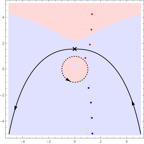
Figure 1: The integration contours (color online). The dashed circle corresponds to the initial contour of integration $C_{>}$. The black solid line represents the steepest descent contour $C_{1}$. The cross marks the position of the saddle point. Red and blue dots correspond to the poles $z_{n}$ defined by Eq. (57) for non-negative and negative indices, respectively. The shaded areas show the regions of positive (pink) and negative (light blue) values of $\mathrm{Re}\,\theta(z)$, see Eq. (51).

The formula (56) allows one immediately to read off the asymptotic behaviour. The residues produce exponentially decaying terms; the leading contribution is given by the smallest real part $\mathrm{Re}\,\theta(z_{n})$. For wide range of the parameters of the model we observed that this achieved for the pole at $z_{0}$. Another type of contribution to the asymptotics comes from the saddle point evaluation of the integral in (56). To find the overall leading contribution we need to compare $\mathrm{Re}\,\theta(z_{0})$ and $\mathrm{Re}\,\theta(z_{\mathrm{sp}})$. This leads to the equation for the critical velocity $v_{c}$ separating two regimes

$$-v_{c}\log(v_{c}+\sqrt{v_{c}^{2}-1})+\sqrt{v_{c}^{2}-1}=-v_{c}\log|z_{0}|+\frac{\pi}{\beta}(1-\kappa).$$ (59)

For $v<v_{c}$ the saddle point is dominating and $T(x,t)$ is given by

$$T(x,t)\approx\frac{S(z_{\rm sp})}{J(z_{\rm sp})+e^{i\pi\kappa}}\frac{e^{-x\log z_{\rm sp}-\frac{it}{2}(z_{\rm sp}+z_{\rm sp}^{-1})}}{\sqrt{2\pi t\sqrt{v^{2}-1}}},$$ (60)

for $v\geq v_{c}$ the pole gives the leading contribution

$$T(x,t)\approx-\frac{2}{\beta}\frac{e^{-i\pi\kappa}}{z_{0}-z_{0}^{-1}}S(z_{0})e^{-x\log z_{0}-\frac{it}{2}(z_{0}+z_{0}^{-1})}.$$ (61)

The asymptotics for the tau function can be found from Eq. (49), for which we also provide the simplified expression for $K(x,t)$

$$\log K(x,t)=2\log Z+ix\int\limits_{-\pi}^{\pi}\nu(q)dq,$$ (62)

where $\nu(q)$ is given by Eqs. (48) and (42). We compare these asymptotic expressions for the correlation functions with numerical evaluation of Fredholm determinants (11) in Fig. 2. We see that asymptotics given by the integral (the red solid line), i.e. by the tau function is hardly distinguishable from the true correlation function even for small $x$.

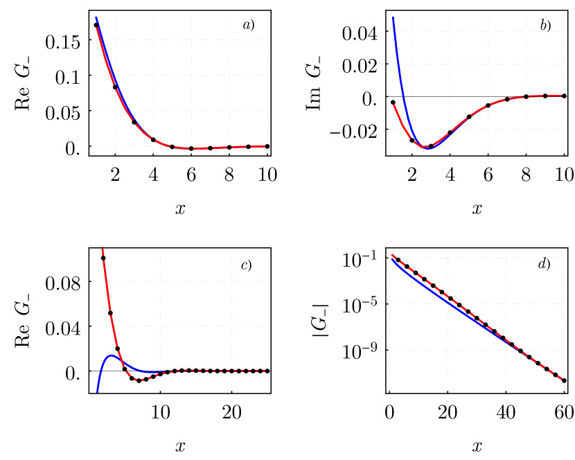
Figure 2: Asymptotic behavior of $G_{-}(x,t)$ for ${\kappa=0.6}$, $h=0.7$, $\beta=2.3$. These parameters correspond to critical velocity $v_{c}\approx 1.676$. Black dots present $G_{-}(x,t)$ computed numerically from (11). Red lines present effective $\tau$ function (49) computed with (48). Blue lines present asymptotics of integrals in (49) given by Eqs. (60), (61). Panels $a)$ and $b)$ correspond to overcritical region $v=2.5$. Panels $c)$ and $d)$ show real part and absolute value of $G_{-}(x,t)$ in the subcritical region $v=1.3$, respectively.

IV.3 Asymptotic behaviour of correlation function in time-like region

Now let us try to apply the same reasoning for the time-like region, $|v|<1$. In this case there are two critical points $q_{1}$ and $q_{2}$

$$\Phi^{\prime}(q_{i})=0,\qquad q_{i}\in[-\pi,\pi),$$ (63)

therefore the approximation (47) naively gives rise to the solution

$$\nu(p)\approx\nu_{\mathrm{sign}\,\Phi^{\prime}(p)}(p),$$ (64)

where $\nu_{\pm}(p)$ are defined by Eqs. (42). This is valid for all $p$ lying far enough from the critical points. Indeed, the approximation (47) holds everywhere outside small vicinities of width $\sim t^{-1/2}$ around critical points $q_{1}$ and $q_{2}$.

It is very tempting to ignore these domains and approximate $\nu(p)$ as a truly discontinuous function, since we are interested in the large $t$ behavior. This procedure however is not consistent with the approximations made in Eq. (44) where we have discarded critical point contributions (the last integral). But even bigger problems appear when one tries to use discontinuous $\nu(p)$ for the asymptotic expression. For instance the double integral (34) is divergent for such a choice.

Therefore, we expect that the solution of the Eq. (40) will have the following “regularized” form

$$\nu(p)=A(p)+B(p)s(p),$$ (65)

where

$$A(p)=\frac{\nu_{+}(p)+\nu_{-}(p)}{2},\qquad B(k)=\frac{\nu_{+}(p)-\nu_{-}(p)}{2},$$ (66)

and the function $s(p)$ is a regularization of $\operatorname{sign}$ function

$$s(p)=f(\sqrt{t}\Phi^{\prime}(p)),$$ (67)

with $f$ being a smooth function satisfying

$$\quad f(\pm\infty)=\pm 1.$$ (68)

So away from the critical points on the distance bigger than $O(1/\sqrt{t})$ we recover the solution (64). We demonstrate this schematically in Fig. 3. Notice that the regularization is needed only for the imaginary parts and the real parts of $\nu_{+}(p)$ and $\nu_{-}(p)$ coincide.

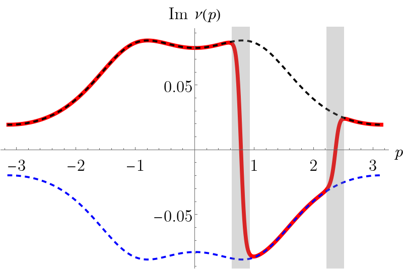
Figure 3: The schematic dependence of the effective phase shift $\nu(p)$. The black and blue dotted lines represent $\nu_{+}(q)$ and $\nu_{-}(q)$, respectively. The red lines shows the regularized expression for $\nu(p)$. The shaded rectangles show the regions where the transition between $\nu_{+}$ and $\nu_{-}$ happens and the regularization is required to approximate $\nu(p)$. These regions are located near critical points $q_{1},q_{2}$ and their widths are $O(t^{-1/2})$. We show only the imaginary part as the real part is continuous and does not require regularization.

Now for the smooth $\nu(p)$ we can use all the results from the previous sections. In particular, we can integrate Eq. (34) by parts to obtain

$$\log Z=\frac{1}{2}\int\limits_{-\pi}^{\pi}dq\int\limits_{-\pi}^{\pi}dk\,\nu^{\prime}(q)\nu^{\prime}(k)\log\left|\sin\frac{q-k}{2}\right|.$$ (69)

We can perform asymptotic analysis of this expression for large $t$ and obtain

$$Z\approx t^{-\frac{1}{2}(\delta_{1}^{2}+\delta_{2}^{2})}\,Z_{\mathrm{reg}},$$ (70)

where $Z_{\mathrm{reg}}$ is $t$-independent factor depending on $s(p)$ and

$$\delta_{1}=\nu_{-}(q_{1})-\nu_{+}(q_{1}),\quad\delta_{2}=\nu_{+}(q_{2})-\nu_{-}(q_{2}).$$ (71)

Therefore the only regularization dependence remains in the overall constant prefactor. It is remarkable that the exponent of power law $t$-dependence of $Z$ is universal (does not depend on the regularization $s(p)$ for any $f$ satisfying (68)). These computations and the exact form for $Z_{\mathrm{reg}}$ are given in the Appendix.

Let us also discuss the asymptotic behavior of the remaining part of the tau function. In there we substitute already discontinuous $\nu(q)$. Namely, we analyze the integral

$$T(x,t)=\int\limits_{-\pi}^{\pi}\frac{dk}{2\pi}n_{F}(k)e^{-it\Phi(k)}e^{-Y(k)},$$ (72)

where

$$Y(k)=\fint\limits_{-\pi}^{\pi}dq\,\nu(q)\cot\frac{q-k}{2}.$$ (73)

The function $Y(k)$ is logarithmically divergent at $q_{1}$ and $q_{2}$ because of discontinuity of $\nu(q)$. It leads to power like singularities in the integrand of (72) which are integrable if $\mathrm{Re}\,\delta_{j}>-\frac{1}{2}$. In our case $\nu_{+}(k)$ and $\nu_{-}(k)$ are conjugate to each other rendering the real part of effective phase shift to be continuous, $\mathrm{Re}\,\delta_{j}=0$.

We separate a regular part $\tilde{Y}(k)$ of $Y(k)$ as

$$Y(k)=\tilde{Y}(k)+(\nu_{-}(k)-\nu_{+}(k))\log\left(\frac{\sin\frac{q_{1}-k}{2}}{\sin\frac{q_{2}-k}{2}}\right)^{2},$$ (74)

$$\tilde{Y}(k)=\int\limits_{-\pi}^{q_{1}}dq\,(\nu_{+}(q)-\nu_{+}(k))\cot\frac{q-k}{2}\\ +\int\limits_{q_{1}}^{q_{2}}dq\,(\nu_{-}(q)-\nu_{-}(k))\cot\frac{q-k}{2}\\ +\int\limits_{q_{2}}^{\pi}dq\,(\nu_{+}(q)-\nu_{+}(k))\cot\frac{q-k}{2}.$$ (75)

Now all is prepared to find the asymptotic behaviour of $T(x,t)$ for large $x$ and $t$ coming from the contributions of two critical points $q_{1}$ and $q_{2}$

$$T(x,t)\approx T_{1}+T_{2},$$ (76)

where

$$T_{j}=\frac{n_{F}(q_{j})}{2\pi}e^{-it\Phi(q_{j})-\tilde{Y}(q_{j})}\left(2\sin\frac{q_{2}-q_{1}}{2}\right)^{-2\delta_{j}}\\ \times\left(\frac{it\Phi^{\prime\prime}(q_{j})}{2}\right)^{-\frac{1}{2}-\delta_{j}}\Gamma\left(\frac{1}{2}+\delta_{j}\right).$$ (77)

The final formula for the asymptotics of the correlation function $G_{-}(x,t)$ is

$$G_{-}(x,t)\approx R_{\infty}T(x,t)t^{-\delta_{1}^{2}-\delta_{2}^{2}}e^{iht}\\ \times\exp\left(i\int_{-\pi}^{\pi}(x-t\sin q)\nu(q)dq\right),$$ (78)

where $R_{\infty}$ is a constant different on each ray $v=x/t$ that additionally depends on the parameters $\kappa$, $h$ and inverse temperature $\beta$. To check this asymptotics we plot in Fig. 4 the ratio $R(x,t)$ of $G_{-}(x,t)$ calculated numerically from (11) to the asymptotics from the right-hand side of Eq. (78) without $R_{\infty}$. We observe that it approaches a constant value. The possible deviations are of order $O(1/\sqrt{t})$, which is consistent with our approximations made for the $\nu(k)$. It would be interesting to see if these corrections can be interpreted in terms of the non-linear Luttinger liquid paradigm [73, 74].

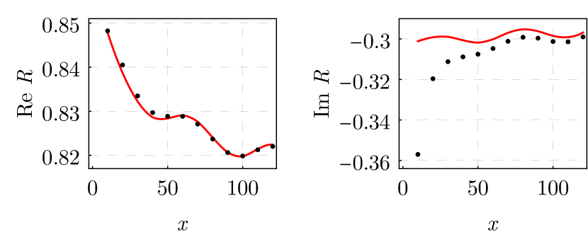
Figure 4: Real and imaginary part of $R(x,t)$ with $v=x/t=0.5$, $\kappa=0.6$, $h=0.7$ and $\beta=2.3$. Red line present $R(x,t)$ for which the integral $T(x,t)$ in Eq. (72) computed exactly. Black dots present $R(x,t)$ for which we use asymptotics of integral $T(x,t)$ given by Eq. (76).

V Summary and Outlook

In this paper we found asymptotics of dynamical correlation functions of anyonic gas with the parameter of anyonic statistics $0\leq\kappa<1$ using recently introduced [43] effective form factor approach. The main difficulty of this method is to find the phase shift function $\nu(q)$ for effective fermions solving an integral equation. For large $x$ and $t$ we found approximate solutions for this integral equation which depend on the ratio $v=x/t$. For the space-like region, $v>1$, the solution $\nu(q)$ can be approximated by the smooth function $\nu_{+}(q)$. In this case the asymptotics of the correlation function is given by asymptotic analysis of integrals producing the leading contribution either from a pole or from a saddle point. In the case of saddle-point contribution there is an additional power factor correcting the exponential decay of the correlation function.

For the time-like region, $|v|<1$, we approximate the solution $\nu(q)$ for a large finite $t$ by a function having discontinuities at critical points and corresponding to the solution of integral equation at $t=\infty$. Unfortunately this approximate solution can not be used directly to find the asymptotics of correlation function by the methods of [43], since the latter requires a smooth $\nu(q)$. For large finite $t$ we consider a class of regularized $\nu(q)$ having the same limit at $t=\infty$ as the genuine solution. It is remarkable, that the regularized $\nu(q)$ lead to the same asymptotics up to a prefactor independent of $t$. This universal time dependence of asymptotics has an additional power-like factor to the exponential decay of the correlation function. The exponent of this power-like factor is related directly to the jumps of $\nu(q)$ at critical points. We hope that the use of a better approximation to $\nu(q)$ as a solution of the integral equation for a large finite $t$ will fix the exact form of the constant prefactor. Further analysis of the correlation functions in the time-like region by the method of effective form factors will be presented in future publications.

The limiting case $\kappa=1$ of the model corresponds to the quantum XX spin chain model studied intensively in literature. Therefore it is interesting to look at the limits of our results as $\kappa\to 1$ and compare with the known formulas. For the paramagnetic phase, $h>1$, in time-like region the results for the asymptotics were obtained in [75] up to an overall constant depending on $\beta$ and $h$. Our results have the same structure as a function of $t$. The ferromagnetic phase, $h<1$, was studied in [76, 19, 20] in space-like region and [76] in time-like region. Unfortunately, the direct application of our approach is not possible due to appearance of singularities of $\nu_{\pm}(q)$ at $q=\pm\arccos h$, where $\varepsilon(q)=0$. We believe that these singularities can be properly resolved. But one needs to develop a more delicate limiting procedure, on which we hope to report in the nearest future.

An important ingredient in the derivation of asymptotics in [76, 75, 1] is the use of fact that the correlation function satisfies differential-difference equations of Ablowitz–Ladik integrable system. It would be interesting to generalize this approach to the correlation functions with arbitrary anyonic parameter $\kappa$ and determine precise $v$ dependence of $R_{\infty}$ in Eq. (78).

Another important application of our approach is to use it to describe the scaling behavior of the correlation functions of the anyonic gas. One has to be able to reproduce results for the asymptotics obtained in [77, 78, 79]. Recently, using effective form factors, the finite temperature tau function for the continuum case was investigated in [80].

*

Appendix A Regularization of the prefactor and power-like behaviour

In this Appendix we describe a regularization of the divergent integral

$$\mathcal{A}=\log Z=\frac{1}{2}\int\limits_{-\pi}^{\pi}dq\int\limits_{-\pi}^{\pi}dp\,\nu^{\prime}(q)\nu^{\prime}(k)\log\left|\sin\frac{q-k}{2}\right|$$ (79)

for the case of discontinuous $\nu(k)$. We use the regularization described in Eqs. (65) – (68) and find asymptotics of this integral for large times.

It is natural to divide the derivative of $\nu$ into two parts

$$\nu^{\prime}(k)=\nu^{\prime}_{0}(k)+\nu^{\prime}_{1}(k),$$ (80)

where

$$\nu^{\prime}_{0}(k)=A^{\prime}(k)+B^{\prime}(k)s(k),\quad\nu^{\prime}_{1}(k)=B(k)s^{\prime}(k).$$ (81)

In the large $t$ limit $\nu^{\prime}_{0}(k)$ is a bounded function meanwhile $\nu^{\prime}_{1}(k)$ becomes proportional to $\delta$-function. The double integral $\mathcal{A}$ can be presented as a sum of four parts

$$\mathcal{A}=\mathcal{A}_{00}+\mathcal{A}_{01}+\mathcal{A}_{10}+\mathcal{A}_{11},$$ (82)

where

$$\mathcal{A}_{ij}=\frac{1}{2}\int\limits_{-\pi}^{\pi}dq\int\limits_{-\pi}^{\pi}dp\,\nu^{\prime}_{i}(q)\nu^{\prime}_{j}(k)\log\left|\sin\frac{q-k}{2}\right|.$$ (83)

Note, only $\mathcal{A}_{11}$ part is responsible for the divergence of $\mathcal{A}$ at large $t$. The parts $\mathcal{A}_{00}$, $\mathcal{A}_{01}$ and $\mathcal{A}_{10}$ have non-singular limiting values at $t\to\infty$ which do not depend on regularization of $\nu(k)$. We have

$$\mathcal{A}_{00}\approx\frac{1}{2}\int\limits_{-\pi}^{\pi}dq\int\limits_{-\pi}^{\pi}dp\,[\nu^{\prime}](q)[\nu^{\prime}](k)\log\left|\sin\frac{q-k}{2}\right|$$ (84)

with

$$[\nu^{\prime}](k)=A^{\prime}(k)+B^{\prime}(k)\operatorname{sign}\Phi^{\prime}(k).$$ (85)

Due to $k\leftrightarrow q$ symmetry we have $\mathcal{A}_{01}=\mathcal{A}_{10}$. In the limit $t\to\infty$ the function $\nu^{\prime}_{1}(k)$ becomes a sum of two delta functions and therefore

$$\mathcal{A}_{01}=\mathcal{A}_{10}\approx B_{1}r_{1}\int\limits_{-\pi}^{\pi}dq\,[\nu^{\prime}](q)\log\left|\sin\frac{q-q_{1}}{2}\right|\\ +B_{2}r_{2}\int\limits_{-\pi}^{\pi}dq\,[\nu^{\prime}](q)\log\left|\sin\frac{q-q_{2}}{2}\right|,$$ (86)

where

$$B_{i}=B(q_{i}),\qquad r_{i}=\operatorname{sign}(\Phi^{\prime\prime}(q_{i}))$$ (87)

To evaluate $\mathcal{A}_{11}$ we divide the integration region $[-\pi,\pi]$ into two pieces ${\Lambda_{1}=[-\pi,p]}$ and $\Lambda_{2}=(p,\pi]$, where point $p$ lies between critical points $q_{1}<p<q_{2}$. This way, the double integral $\mathcal{A}_{11}$ is divided into four parts

$$\mathcal{A}_{11}=a_{11}+a_{12}+a_{21}+a_{22},$$ (88)

where

$$a_{ij}=\frac{1}{2}\int\limits_{\Lambda_{i}}dq\int\limits_{\Lambda_{j}}dk\,B(q)B(k)\\ \times s^{\prime}(q)s^{\prime}(k)\log\left|\sin\frac{q-k}{2}\right|.$$ (89)

The integrals $a_{21}$ and $a_{12}$ have finite limits at $t\to\infty$

$$a_{12}=a_{21}\approx 2B_{1}B_{2}r_{1}r_{2}\log\sin\frac{q_{2}-q_{1}}{2}.$$ (90)

Remaining parts of $\mathcal{A}_{11}$ contain singularities. Let us show how they emerge on example of $a_{11}$. It is natural to present $a_{11}$ as a sum of two integrals (regular and singular)

$$a_{11}=a_{11}^{(r)}+a_{11}^{(s)},$$ (91)

where

$$a_{11}^{(r)}=\frac{1}{2}\int\limits_{\Lambda_{1}}dq\int\limits_{\Lambda_{1}}dk\,B(q)B(k)\\ \times s^{\prime}(q)s^{\prime}(k)\log\left|\frac{\sin\frac{q-k}{2}}{\Phi^{\prime}(q)-\Phi^{\prime}(k)}\right|,$$ (92)

$$a_{11}^{(s)}=\frac{1}{2}\int\limits_{\Lambda_{1}}dq\int\limits_{\Lambda_{1}}dk\,B(q)B(k)\\ \times s^{\prime}(q)s^{\prime}(k)\log\left|\Phi^{\prime}(q)-\Phi^{\prime}(k)\right|.$$ (93)

The first integral can be found using L’Hôpital’s rule

$$a_{11}^{(r)}=\frac{2r_{1}\cdot 2r_{1}}{2}\int\limits_{\Lambda_{1}}dq\int\limits_{\Lambda_{1}}dk\,B(q)B(k)\delta(q-q_{1})\delta(k-q_{1})\\ \times\log\left|\frac{\sin\frac{q-k}{2}}{\Phi^{\prime}(q)-\Phi^{\prime}(k)}\right|=-2B_{1}^{2}\log|2\Phi^{\prime\prime}(q_{1})|,$$ (94)

where we used $r_{1}^{2}=1$. The second integral can be presented as

$$a_{11}^{(s)}=u_{1}+v_{1}\log\sqrt{t},$$ (95)

where

$$u_{1}=\frac{1}{2}\int\limits_{\Lambda_{1}}dq\int\limits_{\Lambda_{1}}dk\,B(q)B(k)\\ \times s^{\prime}(q)s^{\prime}(k)\log\left|\sqrt{t}\Phi^{\prime}(q)-\sqrt{t}\Phi^{\prime}(k)\right|,$$ (96)

$$v_{1}=-\frac{1}{2}\int\limits_{\Lambda_{1}}dq\int\limits_{\Lambda_{1}}dk\,B(q)B(k)s^{\prime}(q)s^{\prime}(k).$$ (97)

Performing rescaling of the integration variables one can persuade oneself that in under the last integrals $B(q)$ can be replaced to $B_{1}$, which leads to

$$v_{1}=-\frac{B_{1}^{2}}{2}\int\limits_{\Lambda_{1}}dq\int\limits_{\Lambda_{1}}dk\,s^{\prime}(q)s^{\prime}(k)=-2B_{1}^{2}.$$ (98)

Here we have used (68), and all the traces of the regularization has disappeared. With $u_{1}$ this will not be the same. Indeed, using $s(k)=f(\sqrt{t}\Phi^{\prime}(k))$ and changing the variables of integration $q$ and $k$ by $\lambda=\sqrt{t}\Phi^{\prime}(q)$ and $\mu=\sqrt{t}\Phi^{\prime}(k)$ we get

$$u_{1}=\frac{1}{2}\int\limits_{\tilde{\Lambda}_{1}}d\lambda\int\limits_{\tilde{\Lambda}_{1}}d\mu\,b(\lambda)b(\mu)f^{\prime}(\lambda)f^{\prime}(\mu)\log|\lambda-\mu|,$$ (99)

where the function $b(\lambda)$ is defined as

$$b(\sqrt{t}\Phi^{\prime}(q))=B(q)$$ (100)

and region $\tilde{\Lambda}_{1}$ is the segment $[\sqrt{t}\Phi^{\prime}(-\pi),\sqrt{t}\Phi^{\prime}(p)]$ which becomes the real line when $t$ goes to infinity. Also $b(\lambda)$ goes to $B_{1}$ at $t\to\infty$. Therefore we get

$$u_{1}\approx\frac{B_{1}^{2}}{2}\cdot\int\limits_{-\infty}^{\infty}d\lambda\int\limits_{-\infty}^{\infty}d\mu\,f^{\prime}(\lambda)f^{\prime}(\mu)\log|\lambda-\mu|.$$ (101)

Finally, using $B_{1}=-\delta_{1}/2$, $B_{2}=\delta_{2}/2$, $r_{1}=-1$, $r_{2}=1$ we obtain the following large $t$ asymptotics of $\mathcal{A}$

$$\mathcal{A}\approx d_{0}+d_{1}\log\sqrt{t},$$ (102)

where the constant $d_{1}$ is universal, i.e. it is independent of regularizing function $f$

$$d_{1}=-2(B_{1}^{2}+B_{2}^{2})=-\frac{1}{2}(\delta_{1}^{2}+\delta_{2}^{2})$$ (103)

and $d_{0}$ depends on a regularizing function $f$ only in summands $u_{1}$ and $u_{2}$

$$d_{0}=\mathcal{A}_{00}+2\mathcal{A}_{01}+2a_{12}+a_{11}^{(r)}+a_{22}^{(r)}+u_{1}+u_{2}.$$ (104)

References

- Korepin et al. [1993] V. E. Korepin, N. M. Bogoliubov, and A. G. Izergin, Quantum Inverse Scattering Method and Correlation Functions, Cambridge Monographs on Mathematical Physics (Cambridge University Press, 1993).
- Tsvelik [2003] A. M. Tsvelik, Quantum Field Theory in Condensed Matter Physics (Cambridge University Press, 2003).
- Giamarchi [2003] T. Giamarchi, Quantum Physics in One Dimension (Oxford University Press, 2003).
- Cazalilla et al. [2011] M. A. Cazalilla, R. Citro, T. Giamarchi, E. Orignac, and M. Rigol, One dimensional bosons: From condensed matter systems to ultracold gases, Rev. Mod. Phys. 83, 1405 (2011).
- Bloch [2005] I. Bloch, Ultracold quantum gases in optical lattices, Nature Physics 1, 23 (2005).
- Kinoshita et al. [2006] T. Kinoshita, T. Wenger, and D. S. Weiss, A quantum Newton's cradle, Nature 440, 900 (2006).
- Hofferberth et al. [2007] S. Hofferberth, I. Lesanovsky, B. Fischer, T. Schumm, and J. Schmiedmayer, Non-equilibrium coherence dynamics in one-dimensional bose gases, Nature 449, 324 (2007).
- Polkovnikov et al. [2011] A. Polkovnikov, K. Sengupta, A. Silva, and M. Vengalattore, Colloquium: Nonequilibrium dynamics of closed interacting quantum systems, Rev. Mod. Phys. 83, 863 (2011).
- Caux and Essler [2013] J.-S. Caux and F. H. L. Essler, Time evolution of local observables after quenching to an integrable model, Phys. Rev. Lett. 110, 257203 (2013).
- Caux [2016] J.-S. Caux, The Quench Action, Journal of Statistical Mechanics: Theory and Experiment 2016, 064006 (2016).
- Castro-Alvaredo et al. [2016] O. A. Castro-Alvaredo, B. Doyon, and T. Yoshimura, Emergent hydrodynamics in integrable quantum systems out of equilibrium, Phys. Rev. X 6, 041065 (2016).
- Bertini et al. [2016] B. Bertini, M. Collura, J. De Nardis, and M. Fagotti, Transport in out-of-equilibrium XXZ chains: Exact profiles of charges and currents, Phys. Rev. Lett. 117, 207201 (2016).
- Nardis et al. [2021] J. D. Nardis, B. Doyon, M. Medenjak, and M. Panfil, Correlation functions and transport coefficients in generalised hydrodynamics (2021), arXiv:2104.04462 [cond-mat.stat-mech] .
- Dugave et al. [2013] M. Dugave, F. Göhmann, and K. K. Kozlowski, Thermal form factors of the XXZ chain and the large-distance asymptotics of its temperature dependent correlation functions, Journal of Statistical Mechanics: Theory and Experiment 2013, P07010 (2013).
- Dugave et al. [2014] M. Dugave, F. Göhmann, and K. K. Kozlowski, Low-temperature large-distance asymptotics of the transversal two-point functions of the XXZ chain, Journal of Statistical Mechanics: Theory and Experiment 2014, P04012 (2014).
- Göhmann [2020] F. Göhmann, Statistical mechanics of integrable quantum spin systems, SciPost Phys. Lect. Notes , 16 (2020).
- Göhmann et al. [2017] F. Göhmann, M. Karbach, A. Klümper, K. K. Kozlowski, and J. Suzuki, Thermal form-factor approach to dynamical correlation functions of integrable lattice models, Journal of Statistical Mechanics: Theory and Experiment 2017, 113106 (2017).
- Göhmann et al. [2020a] F. Göhmann, K. K. Kozlowski, and J. Suzuki, High-temperature analysis of the transverse dynamical two-point correlation function of the XX quantum-spin chain, Journal of Mathematical Physics 61, 013301 (2020a).
- Göhmann et al. [2019] F. Göhmann, K. K. Kozlowski, J. Sirker, and J. Suzuki, Equilibrium dynamics of the XX chain, Phys. Rev. B 100, 155428 (2019).
- Göhmann et al. [2020b] F. Göhmann, K. K. Kozlowski, and J. Suzuki, Long-time large-distance asymptotics of the transverse correlation functions of the XX chain in the spacelike regime, Letters in Mathematical Physics 110, 1783 (2020b).
- Its et al. [1990] A. Its, A. Izergin, V. Korepin, and N. Slavnov, Differential Equations For Quantum Correlation Functions, International Journal of Modern Physics B 04, 1003 (1990).
- Price [2017] T. Price, Long time thermal asymptotics of nonlinear Luttinger liquid from inverse scattering, arXiv preprint arXiv:1708.02170 (2017).
- LeClair and Mussardo [1999] A. LeClair and G. Mussardo, Finite temperature correlation functions in integrable QFT, Nuclear Physics B 552, 624 (1999).
- Saleur [2000] H. Saleur, A comment on finite temperature correlations in integrable QFT, Nuclear Physics B 567, 602 (2000).
- Mussardo [2001] G. Mussardo, On the finite temperature formalism in integrable quantum field theories, Journal of Physics A: Mathematical and General 34, 7399 (2001).
- Castro-Alvaredo and Fring [2002] O. Castro-Alvaredo and A. Fring, Finite temperature correlation functions from form factors, Nuclear Physics B 636, 611 (2002).
- Doyon [2005] B. Doyon, Finite-temperature form factors in the free Majorana theory, Journal of Statistical Mechanics: Theory and Experiment 2005, P11006 (2005).
- Altshuler et al. [2006] B. Altshuler, R. Konik, and A. Tsvelik, Low temperature correlation functions in integrable models: Derivation of the large distance and time asymptotics from the form factor expansion, Nuclear Physics B 739, 311 (2006).
- Doyon [2007] B. Doyon, Finite-Temperature Form Factors: a Review, Symmetry, Integrability and Geometry: Methods and Applications 10.3842/sigma.2007.011 (2007).
- Essler and Konik [2009] F. H. L. Essler and R. M. Konik, Finite-temperature dynamical correlations in massive integrable quantum field theories, Journal of Statistical Mechanics: Theory and Experiment 2009, P09018 (2009).
- Pozsgay and Takács [2010] B. Pozsgay and G. Takács, Form factor expansion for thermal correlators, Journal of Statistical Mechanics: Theory and Experiment 2010, P11012 (2010).
- Perfetto and Doyon [2021] G. Perfetto and B. Doyon, Euler-scale dynamical fluctuations in non-equilibrium interacting integrable systems, SciPost Phys. 10, 116 (2021).
- Cubero and Panfil [2019] A. C. Cubero and M. Panfil, Thermodynamic bootstrap program for integrable QFT’s: form factors and correlation functions at finite energy density, Journal of High Energy Physics 2019, 10.1007/jhep01(2019)104 (2019).
- Cubero and Panfil [2020] A. C. Cubero and M. Panfil, Generalized hydrodynamics regime from the thermodynamic bootstrap program, SciPost Physics 8, 10.21468/scipostphys.8.1.004 (2020).
- Cubero [2020] A. C. Cubero, How generalized hydrodynamics time evolution arises from a form factor expansion, arXiv preprint arXiv:2001.03065 (2020).
- Nardis and Panfil [2015] J. D. Nardis and M. Panfil, Density form factors of the 1D Bose gas for finite entropy states, Journal of Statistical Mechanics: Theory and Experiment 2015, P02019 (2015).
- Nardis and Panfil [2016] J. D. Nardis and M. Panfil, Exact correlations in the Lieb–Liniger model and detailed balance out-of-equilibrium, SciPost Phys. 1, 015 (2016).
- Nardis and Panfil [2018] J. D. Nardis and M. Panfil, Particle-hole pairs and density–density correlations in the Lieb–Liniger model, Journal of Statistical Mechanics: Theory and Experiment 2018, 033102 (2018).
- Panfil [2021] M. Panfil, The two particle–hole pairs contribution to the dynamic correlation functions of quantum integrable models, Journal of Statistical Mechanics: Theory and Experiment 2021, 013108 (2021).
- Panfil and Sant’Ana [2021] M. Panfil and F. T. Sant’Ana, The relevant excitations for the one-body function in the Lieb–Liniger model, Journal of Statistical Mechanics: Theory and Experiment 2021, 073103 (2021).
- Granet et al. [2020] E. Granet, M. Fagotti, and F. H. L. Essler, Finite temperature and quench dynamics in the Transverse Field Ising Model from form factor expansions, SciPost Phys. 9, 33 (2020).
- Granet and Essler [2020] E. Granet and F. H. L. Essler, A systematic -expansion of form factor sums for dynamical correlations in the Lieb-Liniger model, SciPost Phys. 9, 82 (2020).
- Gamayun et al. [2021] O. Gamayun, N. Iorgov, and Y. Zhuravlev, Effective free-fermionic form factors and the XY spin chain, SciPost Phys. 10, 70 (2021).
- Pâţu [2015] O. I. Pâţu, Correlation functions and momentum distribution of one-dimensional hard-core anyons in optical lattices, Journal of Statistical Mechanics: Theory and Experiment 2015, P01004 (2015).
- Pâţu et al. [2007] O. I. Pâţu, V. E. Korepin, and D. V. Averin, Correlation functions of one-dimensional Lieb–Liniger anyons, Journal of Physics A: Mathematical and Theoretical 40, 14963 (2007).
- Pâţu et al. [2008a] O. I. Pâţu, V. E. Korepin, and D. V. Averin, One-dimensional impenetrable anyons in thermal equilibrium: I. anyonic generalization of lenard's formula, Journal of Physics A: Mathematical and Theoretical 41, 145006 (2008a).
- Pâţu et al. [2008b] O. I. Pâţu, V. E. Korepin, and D. V. Averin, One-dimensional impenetrable anyons in thermal equilibrium: II. determinant representation for the dynamic correlation functions, Journal of Physics A: Mathematical and Theoretical 41, 255205 (2008b).
- Pâţu et al. [2009a] O. I. Pâţu, V. E. Korepin, and D. V. Averin, One-dimensional impenetrable anyons in thermal equilibrium: III. large distance asymptotics of the space correlations, Journal of Physics A: Mathematical and Theoretical 42, 275207 (2009a).
- Zinner [2015] N. T. Zinner, Strongly interacting mesoscopic systems of anyons in one dimension, Phys. Rev. A 92, 063634 (2015).
- Keilmann et al. [2011] T. Keilmann, S. Lanzmich, I. McCulloch, and M. Roncaglia, Statistically induced phase transitions and anyons in 1d optical lattices, Nature Communications 2, 361 (2011).
- Greschner et al. [2018] S. Greschner, L. Cardarelli, and L. Santos, Probing the exchange statistics of one-dimensional anyon models, Phys. Rev. A 97, 053605 (2018).
- Cardarelli et al. [2016] L. Cardarelli, S. Greschner, and L. Santos, Engineering interactions and anyon statistics by multicolor lattice-depth modulations, Phys. Rev. A 94, 023615 (2016).
- Sträter et al. [2016] C. Sträter, S. C. L. Srivastava, and A. Eckardt, Floquet realization and signatures of one-dimensional anyons in an optical lattice, Phys. Rev. Lett. 117, 205303 (2016).
- Greschner and Santos [2015] S. Greschner and L. Santos, Anyon Hubbard Model in One-Dimensional Optical Lattices, Phys. Rev. Lett. 115, 053002 (2015).
- Aguado et al. [2008] M. Aguado, G. K. Brennen, F. Verstraete, and J. I. Cirac, Creation, manipulation, and detection of abelian and non-abelian anyons in optical lattices, Phys. Rev. Lett. 101, 260501 (2008).
- Duan et al. [2003] L.-M. Duan, E. Demler, and M. D. Lukin, Controlling spin exchange interactions of ultracold atoms in optical lattices, Phys. Rev. Lett. 91, 090402 (2003).
- Micheli et al. [2006] A. Micheli, G. K. Brennen, and P. Zoller, A toolbox for lattice-spin models with polar molecules, Nature Physics 2, 341–347 (2006).
- Jiang et al. [2008] L. Jiang, G. K. Brennen, A. V. Gorshkov, K. Hammerer, M. Hafezi, E. Demler, M. D. Lukin, and P. Zoller, Anyonic interferometry and protected memories in atomic spin lattices, Nature Physics 4, 482–488 (2008).
- Berkovich and Lowenstein [1987] A. Berkovich and J. Lowenstein, Correlation function of the one-dimensional fermi gas in the infinite-coupling limit (repulsive case), Nuclear Physics B 285, 70 (1987).
- Berkovich [1991] A. Berkovich, Temperature and magnetic field-dependent correlators of the exactly integrable (1+1)-dimensional gas of impenetrable fermions, Journal of Physics A: Mathematical and General 24, 1543 (1991).
- Göhmann et al. [1998a] F. Göhmann, A. Its, and V. Korepin, Correlations in the impenetrable electron gas, Physics Letters A 249, 117 (1998a).
- Izergin and Pronko [1998] A. Izergin and A. Pronko, Temperature correlators in the two-component one-dimensional gas, Nuclear Physics B 520, 594 (1998).
- Göhmann et al. [1998b] F. Göhmann, A. G. Izergin, V. E. Korepin, and A. G. Pronko, Time and temperature dependent correlation functions of the one-dimensional impenetrable electron gas, International Journal of Modern Physics B 12, 2409 (1998b).
- Cheianov and Zvonarev [2004a] V. V. Cheianov and M. B. Zvonarev, Nonunitary spin-charge separation in a one-dimensional fermion gas, Phys. Rev. Lett. 92, 176401 (2004a).
- Fiete and Balents [2004] G. A. Fiete and L. Balents, Green’s function for magnetically incoherent interacting electrons in one dimension, Phys. Rev. Lett. 93, 226401 (2004).
- Cheianov and Zvonarev [2004b] V. V. Cheianov and M. B. Zvonarev, Zero temperature correlation functions for the impenetrable fermion gas, Journal of Physics A: Mathematical and General 37, 2261 (2004b).
- Pâţu [2019] O. I. Pâţu, Correlation functions of one-dimensional strongly interacting two-component gases, Phys. Rev. A 100, 063635 (2019).
- Zvonarev et al. [2008] M. Zvonarev, V. Cheianov, and T. Giamarchi, Time-dependent correlation function of the Jordan–Wigner operator as a Fredholm determinant, Journal of Statistical Mechanics Theory and Experiment 2009 (2008).
- Gamayun et al. [2016] O. Gamayun, A. G. Pronko, and M. B. Zvonarev, Time and temperature-dependent correlation function of an impurity in one-dimensional Fermi and Tonks–Girardeau gases as a Fredholm determinant, New Journal of Physics 18, 045005 (2016).
- Gamayun et al. [2015] O. Gamayun, A. G. Pronko, and M. B. Zvonarev, Impurity Green’s function of a one-dimensional Fermi gas, Nuclear Physics B 892, 83 (2015).
- Gamayun et al. [2018] O. Gamayun, O. Lychkovskiy, E. Burovski, M. Malcomson, V. V. Cheianov, and M. B. Zvonarev, Impact of the injection protocol on an impurity’s stationary state, Phys. Rev. Lett. 120, 220605 (2018).
- Gamayun et al. [2020] O. Gamayun, O. Lychkovskiy, and M. B. Zvonarev, Zero temperature momentum distribution of an impurity in a polaron state of one-dimensional Fermi and Tonks–Girardeau gases, SciPost Phys. 8, 53 (2020).
- Imambekov and Glazman [2009] A. Imambekov and L. I. Glazman, Universal Theory of Nonlinear Luttinger Liquids, Science 323, 228 (2009).
- Imambekov et al. [2012] A. Imambekov, T. L. Schmidt, and L. I. Glazman, One-dimensional quantum liquids: Beyond the Luttinger liquid paradigm, Rev. Mod. Phys. 84, 1253 (2012).
- Jie [1998] X. Jie, Ph.D. thesis, Indiana University - Purdue University Ph.D. Thesis (1998).
- Its et al. [1993] A. R. Its, A. G. Izergin, V. E. Korepin, and N. A. Slavnov, Temperature correlations of quantum spins, Phys. Rev. Lett. 70, 1704 (1993).
- Pâţu et al. [2009b] O. I. Pâţu, V. E. Korepin, and D. V. Averin, Large-distance asymptotic behavior of the correlation functions of 1d impenetrable anyons at finite temperatures, EPL (Europhysics Letters) 86, 40001 (2009b).
- Pâţu et al. [2010] O. I. Pâţu, V. E. Korepin, and D. V. Averin, One-dimensional impenetrable anyons in thermal equilibrium: IV. large time and distance asymptotic behavior of the correlation functions, Journal of Physics A: Mathematical and Theoretical 43, 115204 (2010).
- Santachiara and Calabrese [2008] R. Santachiara and P. Calabrese, One-particle density matrix and momentum distribution function of one-dimensional anyon gases, Journal of Statistical Mechanics: Theory and Experiment 2008, P06005 (2008).
- Chernowitz and Gamayun [2021] D. Chernowitz and O. Gamayun, On the dynamics of free-fermionic tau-functions at finite temperature (2021), arXiv:2110.08194 [cond-mat.stat-mech] .