The Magnetic Origin of Solar Campfires

Abstract

Solar campfires are fine-scale heating events, recently observed by Extreme Ultraviolet Imager (EUI), onboard Solar Orbiter. Here we use EUI 174Å images, together with EUV images from SDO/AIA, and line-of-sight magnetograms from SDO/HMI to investigate the magnetic origin of 52 randomly selected campfires in the quiet solar corona. We find that (i) the campfires are rooted at the edges of photospheric magnetic network lanes; (ii) most of the campfires reside above the neutral line between majority-polarity magnetic flux patch and a merging minority-polarity flux patch, with a flux cancelation rate of $\sim$10¹⁸Mx hr^-1; (iii) some of the campfires occur repeatedly from the same neutral line; (iv) in the large majority of instances, campfires are preceded by a cool-plasma structure, analogous to minifilaments in coronal jets; and (v) although many campfires have ‘complex’ structure, most campfires resemble small-scale jets, dots, or loops. Thus, ‘campfire’ is a general term that includes different types of small-scale solar dynamic features. They contain sufficient magnetic energy ($\sim$10²⁶-10²⁷ erg) to heat the solar atmosphere locally to 0.5–2.5MK. Their lifetimes range from about a minute to over an hour, with most of the campfires having a lifetime of $<$10 minutes. The average lengths and widths of the campfires are 5400$\pm$2500km and 1600$\pm$640km, respectively. Our observations suggest that (a) the presence of magnetic flux ropes may be ubiquitous in the solar atmosphere and not limited to coronal jets and larger-scale eruptions that make CMEs, and (b) magnetic flux cancelation is the fundamental process for the formation and triggering of most campfires.

1 Introduction

The Solar Orbiter mission was launched on 10 February 2020 (Müller et al., 2020). The payload consists of six remote sensing and four in-situ instruments. One of its instruments, the Extreme Ultraviolet Imager (EUI; Rochus et al. 2020) has two High Resolution Imagers (HRIs): HRI_EUV and HRI_Lya. Both the HRIs observed the quiet solar corona, in the 174 Å and 1216 Å passbands, during the first perihelion pass of Solar Orbiter. The HRI_EUV captured small-scale brightenings, known as campfires (Berghmans et al., 2021), on the solar disk center in 174 Å images.

Solar campfires are small-scale, short-lived, coronal brightenings, and can appear as loop-like, dot-like or complex structures. They are mostly rooted at the chromospheric network boundaries and their height lies between 1000 and 5000 km above the photosphere (Berghmans et al., 2021; Zhukov et al., 2021). The formation mechanisms of campfires and their connection to the photospheric magnetic field are unknown.

Campfires might be magnetic reconnection events in the quiet Sun corona, at small-scales, in low-lying magnetic structures. Therefore, these could intrinsically be similar to sub-flares (nanoflares, microflares) and larger-scale solar eruptions (Parker, 1988; Priest & Forbes, 2000; Aschwanden, 2004). Consistently, Chen et al. (2021) proposed, using an MHD model, that campfires are mostly caused by component magnetic reconnection, heating the quiet Sun corona to 1 MK or more.

In this Letter, we examine the magnetic field evolution at the base of campfires and investigate what triggers these heating events. We also examine the physical properties of campfires. For this purpose, we combine the HRI_EUV  images with images of Solar Dynamics Observatory (SDO)/Atmospheric Imaging Assembly (AIA; Lemen et al. 2012), and investigate the photospheric magnetic field evolution of ondisk campfires using co-aligned line of sight magnetograms from SDO/Helioseismic and Magnetic Imager (HMI; Scherrer et al. 2012). By studying a total of 52 campfires observed at 44 different locations, we find that (i) 77% (40 out of 52) of campfires appear at sites of magnetic flux cancelation between the majority-polarity flux patch and a merging minority-polarity flux patch, and (ii) 79% (41 out of 52) of campfires are accompanied by structures of cool plasma.

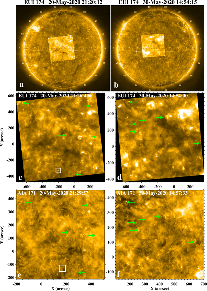
Figure 1: Examples of campfires observed on 20-May-2020 and 30-May-2020. Panels (a) and (b) show the EUI/Full Sun Imager (FSI) 174 Å images overlaid with the High Resolution Imager (HRI) field of view. The intersections of the two solid yellow circles in (a) and (b) indicate the SDO subsolar points. Panels (c) and (d) show the HRI_EUV images of the same region that is overlaid in panels (a) and (b), respectively. Panels (e) and (f) display AIA 171 Å images of the same field of view shown in panels (c) and (d). The green arrows (in c and d) point to some of the campfires that we have studied. The green arrows in the AIA images point to the same campfires. The white box in HRI_EUV image (shown in c; also displayed in e) shows the location of the campfires that is presented in detail in Figure 2.

2 DATA and Methods

In this study, we use L2 EUI data (calibrated images) from 20-May-2020 and 30-May-2020. The L2 data is the latest calibrated data product, which is suitable for scientific analysis. The observations of these two days were taken when the instrument was in the commissioning phase. The HRI of EUI captured images in 174 Å channel (centered on the Fe IX and Fe X lines formed around 1 MK) with high spatial resolution (pixel size of 0″.492; Rochus et al. 2020) and high temporal cadence (5 to 10 s). All the campfires we studied here were detected in HRI_EUV 174 Å. None of the campfires were visible in HRI_Lya.

On 20-May-2020, the Solar Orbiter was located at a distance of 0.612 AU from the Sun, which means it observed the Sun from that location with a pixel size of 217 km (Figure 1a). As part of technical compression tests, HRI_EUV produced 174 Å images between 21:20 and 22:17 UT, cycling through a 2 minute program that took 5 images at 10s cadence plus a 6th image 70 s later. These images have variable settings but 60 images are well exposed, un-binned and compressed at high quality levels. We find that campfires are visible in some binned data as well. Therefore, we have kept in the movies all the EUI frames including binned ones.

Whereas on 30-May-2020, the Solar Orbiter was positioned at a distance of 0.556 AU from the Sun (a pixel size of 198 km; Figure 1b) and it captured the HRI_EUV  images for about 5 minutes at every 5 s. Figures 1a and 1b show the EUI/Full Sun Imager (FSI) 174 Å images overlaid with HRI field of view, respectively, for 20-May-2020 and 30-May-2020. Both the images were created with the use of JHelioviewer software (Müller et al., 2017).

In addition to EUI data, we used EUV images from SDO/AIA. AIA provides full-disk solar images in seven different EUV channels. The AIA images have 0″.6 pixels and 12 s temporal cadence. For our analysis, we mainly used 304, 171, 193, and 211 Å images, because we were able to recognize the EUI events clearly in these four channels. We found that campfires are rarely visible in hotter AIA channels (e.g. 335 and 94 Å). We also checked that they are hardly visible in AIA’s UV channels (1600 and 1700 Å). To investigate the photospheric magnetic field setting of campfires, we used line of sight magnetograms, of 45s series, from SDO/HMI. The HMI has 0″.5 pixels, 45 s temporal cadence and a noise level of about 7 G (Schou et al., 2012; Couvidat et al., 2016). Two consecutive magnetograms have been summed at each time step to enhance the visibility of weak field regions.

We downloaded two hours of AIA and HMI data for 20-May-2020 and an hour data for 30-May-2020, using JSOC data cutout service. The AIA and HMI data sets have been co-aligned using SolarSoft routines (Freeland & Handy, 1998). It is important to note that EUI and AIA observed the Sun from different heliocentric distances. Solar Orbiter was at 0.612 AU and 0.556 AU from the Sun on 20-May-2020 and 30-May-2020, respectively. Therefore, the events would appear 3.22 minutes and 3.68 minutes earlier in EUI images than in the AIA images on 20-May-2020 and 30-May-2020, respectively. We have created movies, using EUI, AIA, and HMI data, to follow the evolution of campfires together with their underlying magnetic field. The movies and their corresponding figures display the same field of view. The contours, of $\pm$15 G, of HMI magnetograms are overplotted in the movies and figures. The Differential Emission Measure (DEM; Cheung et al. 2015) has been computed, using six AIA channels (171, 193, 211, 131, 335, and 94 Å), to investigate the emission of campfires in different temperature bins.

We inspected the full-resolution HRI_EUV data and manually identified 52 campfires (from 44 different locations). We looked for those events that show similarities with the campfires in the Solar Orbiter/EUI press release images. After selecting the campfires in HRI_EUV 174 Å, we looked for the same campfires in the AIA 171 Å images. Then we co-aligned, using solar soft routines, the HMI line of sight magnetograms with respect to the AIA images, both onboard SDO. Therefore, the alignment between AIA images and HMI magnetograms is accurate in order to study the photospheric magnetic field of the campfires.

Our selected campfires are also consistent with the categories of campfires (loop-like, dot-like, and complex) in Berghmans et al. (2021). In addition, we find several campfires to be jet-like in their appearance. All of our selected events are listed in Table 1. We find that some of the campfires occur more than once from the same location. We mainly obtained the duration, length, and width of the campfires from the HRI_EUV images. We used AIA data to estimate the duration of those campfires that start/end a few minutes before/after the EUI-time coverage.

In Table 1, the measured length is the integrated distance of each campfire along their longer-extension, whereas the estimated width is the cross-sectional distance of the campfire. Both measurements are taken during the peak brightening of the campfires in HRI_EUV images. To estimate the uncertainty in the length and width, we repeated the measurements three times at three nearby locations and then took average of the three measurements. The listed uncertainty is the uncertainty of the mean (that is, standard deviation of the three measured lengths/widths from their mean, divided by the square root of 3). The duration of campfires is the estimated time from when each of the campfire turns on until when it fades away in HRI_EUV images.

In Table 1 we have also listed the visibility of cool-plasma that is confirmed from the AIA 304 Å and/or 171 Å images. We also mention the category of campfires in the last column – the events appear as loop-like, dot-like, jet-like, or complex structures.

We created magnetic flux evolution plots to quantitatively assess the changes in magnetic flux as a function of time. We integrate flux inside a box covering those magnetic patches that are usually easier to isolate from the neighboring magnetic flux elements, and make sure no opposite flux flows across the boundary of the box. Furthermore, we also created HMI time-distance flux maps to present a detailed and clear picture of magnetic field evolution (e.g., Figure 3b).

Table 1: Measured Parameters of the Observed Campfires

Event	Time	Location	No. of	Duration	Length	Width	Visibility of	Discernible	Category
No.	(UT)	(x,y)arcsec	CFs	(minutes)	(km)	(km)	cool plasma	flux cancel.	of CFs
20-May-2020
1	21:20:52	-230,-270	3	2.1$\pm$10s	7100$\pm$330	1400$\pm$40	Y	A	loop-like
	21:54:22			6.0 $\pm$12s	7800$\pm$350	1350$\pm$100	Y	A
2	21:26:12	-235,-305	2	7.0$\pm$10s	5700$\pm$340	1500$\pm$160	Y	Y	loop-like
	21:58:22			4.0$\pm$12s	6900$\pm$730	2700$\pm$900	Y	Y
3	21:35:02	-20,-250	3	2.0$\pm$10s	7600$\pm$50	1600$\pm$360	Y	A	loop-like
	21:44:52			1.5$\pm$10s	5500$\pm$150	1300$\pm$100	Y	A
	22:00:52			4.5$\pm$12s	9300$\pm$900	2100$\pm$300	Y	A
4	21:48:22	-580,380	2	7.0$\pm$10s	8700$\pm$550	1700$\pm$670	Y	Y	complex
	22:10:32			2.0$\pm$10s	7000$\pm$640	1300$\pm$50	Y	Y
5	21:26:52	285,55	1	17.0$\pm$20s	5500$\pm$920	2200$\pm$280	Y	Y	complex
6	22:22:42	225,445	1	8.0$\pm$1m	9600$\pm$430	1900$\pm$220	Y	Y	complex
7	21:32:42	-40,-370	2	6.0$\pm$10s	7300$\pm$350	2700$\pm$260	Y	Y	complex
	22:08:12			129$\pm$24s	7000$\pm$550	2400$\pm$300	Y	Y
8	21:37:02	-80,150	1	17.0$\pm$10s	4900$\pm$60	1600$\pm$235	Y	Y	loop-like
9	22:10:22	-600,580	1	12.0$\pm$30s	9500$\pm$280	2600$\pm$295	Y	Y	complex
10	22:13:02	-530,570	1	13.0$\pm$10s	10400$\pm$810	1900$\pm$780	Y	Y	jet-like
11	22:08:12	-590,500	1	8.0$\pm$10s	5000$\pm$160	2000$\pm$225	Y	Y	jet-like
12	22:04:52	-520,510	1	26.0$\pm$20s	8100$\pm$340	1300$\pm$430	Y	Y	dot-like
13	22:11:02	280,43	1	6.5$\pm$10s	6000$\pm$440	3800$\pm$225	Y	Y	jet-like
14	22:16:22	-45,-380	1	9.0$\pm$12s	2900$\pm$150	1400$\pm$250	Y	Y	complex
15	21:38:22	-600,510	1	3.0$\pm$10s	3300$\pm$350	1500$\pm$240	Y	Y	jet-like
16	22:14:52	-580,365	1	8.0$\pm$10s	2700$\pm$350	1800$\pm$160	Y	Y	loop-like
17	22:08:22	-605,395	2	5.5$\pm$10s	3700$\pm$100	1200$\pm$400	Y	Y	jet-like
	22:14:32			2.0$\pm$10s	1300$\pm$150	1100$\pm$100	Y	Y
18	22:00:22	-400,-20	1	1.0$\pm$10s	4900$\pm$570	2800$\pm$150	Y	Y	jet-like
19	22:16:22	-400,0	1	8.0$\pm$12s	2400$\pm$200	2100$\pm$130	Y	Y	dot-like
20	22:11:22	-380,0	1	4.0$\pm$10s	1000$\pm$10	960$\pm$40	Y	Y	dot-like
30-May-2020
21	14:54:40	-450,330	1	7.0$\pm$12s	9600$\pm$670	1100$\pm$315	Y	Y	complex
22	14:54:30	-440,220	2	11.0$\pm$12s	8400$\pm$85	1700$\pm$690	Y	Y	complex
23	14:57:50	-335,145	1	4.0$\pm$5s	4700$\pm$185	1000$\pm$90	Y	A	complex
24	15:04:03	-175,154	1	3.0$\pm$15s	7400$\pm$250	750$\pm$10	Y	Y	loop-like
25	14:56:10	-100,370	1	20.5$\pm$24s	5500$\pm$420	1600$\pm$370	Y	Y	complex
26	14:55:50	-305,350	3	5.0$\pm$12s	4700$\pm$470	1000$\pm$220	Y	Y	jet-like
	15:04:00			3.0$\pm$12s	5800$\pm$450	1200$\pm$100	Y	Y
27	14:55:00	135,47	1	1.5$\pm$5s	4100$\pm$160	900$\pm$75	N	Y	loop-like
28	14:55:55	20,-70	1	3.5$\pm$10s	4300$\pm$140	1000$\pm$120	Y	Y	complex
29	14:54:00	-190,50	1	3.5$\pm$5s	–	–	Y	Y	complex
30	14:55:10	-220,-100	1	198$\pm$10m	6600$\pm$350	2000$\pm$200	A	Y	complex
31	14:54:25	105,-180	1	22$\pm$12s	6700$\pm$1300	2100$\pm$340	A	A	complex
32	14:57:30	265,-180	1	2.0$\pm$5s	3600$\pm$160	1200$\pm$35	Y	Y	complex
33	14:54:45	95,-235	1	7.0$\pm$12s	3600$\pm$135	1200$\pm$190	Y	A	jet-like
34	14:56:05	-615,140	1	18$\pm$24s	3500$\pm$55	1600$\pm$155	A	Y	complex
35	14:57:20	-575,170	3	4.5$\pm$5s	6300$\pm$530	1100$\pm$155	A	Y	loop-like
36	14:57:55	326,16	1	7.0$\pm$5s	3400$\pm$90	1200$\pm$130	A	Y	complex
37	14:54:30	-500,590	1	30$\pm$24s	7700$\pm$380	2700$\pm$250	Y	Y	jet-like
38	14:55:10	-190,353	1	7.0$\pm$10s	6300$\pm$245	1800$\pm$35	Y	Y	complex
39	14:56:50	-410,-235	1	3.0$\pm$5s	5300$\pm$285	1500$\pm$180	A	Y	complex
40	14:54:25	-154,335	1	3.0$\pm$5s	3000$\pm$255	1000$\pm$140	A	A	dot-like
41	14:57:15	-192,160	1	1.5$\pm$5s	2000$\pm$400	1150$\pm$270	Y	Y	complex
42	14:54:45	-148,320	1	1.0$\pm$5s	2100$\pm$140	700$\pm$100	A	A	loop-like
43	14:54:35	-158,300	1	1.3$\pm$5s	1400$\pm$140	800$\pm$160	N	A	dot-like
44	14:57:20	-195,-340	1	1.3$\pm$10s	750$\pm$20	700$\pm$70	-	-	dot-like
average$\pm$1$\sigma$ave				13.2$\pm$30	5400$\pm$2500	1600$\pm$640

Note. —

^aApproximate time of peak brightening in EUI 174 Å images.

^bApproximate location of the campfires in EUI 174 Å images.

^cTotal no. of campfires (CFs) from the same neutral line.

^dDuration of the campfires in EUI 174 Å images.

^eIntegrated length of the campfires during its peak brightening in EUI 174 Å images.

^fCross-sectional width of the campfires during its peak brightening in EUI 174 Å images.

^gWhether or not a cool-plasma structure is present at the base of the campfires in AIA 304 and/or 171 Å images.

^hWhether a discernible flux cancelation occurs at the base of the campfire.

ⁱCategory of the campfires.

^jCanceling minority polarity flux is far from the PIL.

^kEUI 174 Å images are binned during the second event.

^lMultiple structures brighten at the PIL even after the end of the campfire.

^mCancelation between ‘weak’ flux elements.

ⁿFlux coalescence can be seen at 14:53 UT in the negative flux clump during the event.

^oWeak flux elements cancel 10 min before the rise of cool plasma.

^pAmbiguous, there are many substructures making it difficult to estimate.

^qCool plasma appears and disappears.

^rBarely visible in AIA images.

^$\ast$Only those campfires are characterized here that are covered by EUI (e.g. in Event No. 1, the third campfire is not covered by EUI, thus it is not characterized).

^$\star$Duration estimated from AIA 171Å images.

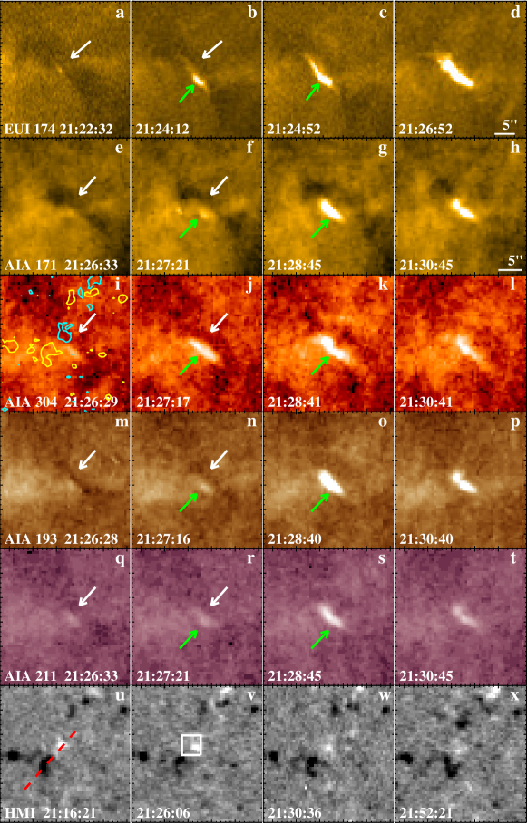
Figure 2: An example of a campfire observed on 20-May-2020. Panels (a-d) show 174 Å HRI_EUV images of the campfire and display the same field of view as inside the white box of Figure 1c. A white horizontal bar in (d) scales 5″ distance for reference. For HRI_EUV on 20-May-2020 1″ is equal to 443 km. Panels (e-h), (i-l), (m-p), and (q-t) show, respectively, the AIA 171, 304, 193, and 211 Å images of the same campfire, and have the same field of view as in the white box of Figure 1e. Panels (u-x) show the HMI line of sight magnetograms of the same region. The diagonal red dashed line in panel (u) show the location of the line along which the time-distance map is created and shown in Figure 3b. The white box in (v) shows the area that is used to calculate the positive magnetic flux plot shown in Figure 3a. The white arrows point to the cool-plasma structure and the green arrows point to the campfire itself. In panel (i), HMI contours, of levels $\pm$15 G (at 21:26:06) are overlaid, where cyan and yellow contours represent the positive and negative magnetic polarities, respectively. Note that EUI events appear 3.2 minutes earlier than in AIA images. The animation (Movie1-AIA) runs from 21:20 to 22:20 UT and the annotations and FOV are same as in this Figure, while the EUI animation (Movie1-So) runs from 21:20 to 21:32 UT and the animation is unannotated.

3 Results

3.1 Overview

Figures 1c and 1d show some of the campfires observed by HRI_EUV on 20-May-2020 and 30-May-2020, respectively. Figures 1e and 1f show the same campfires in AIA 171 Å images. Some of the campfires that we have investigated in detail (listed in Table 1) are marked by green arrows.

All these events appear in AIA 171 and 304 Å images, but not as clearly as in HRI_EUV images (Figure 1). Thus, we likely would not have noticed a few of these features in AIA 171 Å images, without first having them seen in the higher-resolution EUI images. In Section 3.2, we present Campfire-2 of Table 1 in detail, and show six additional campfire examples, including their DEMs, in Appendix (Section 6).

3.2 Presence of Cool Plasma at Campfire’s Base

Figure 2 shows an example of campfire observed on 20-May-2020. As noted in Table 1, there are two campfires from the same location (Campfire-2 of Table 1). Here, we present the first campfire from this location in detail.

Figures 2(a-d) and 2(e-t) show the evolution of the campfire in HRI_EUV and AIA images, respectively. The campfire starts to brighten at 21:24:12 in HRI_EUV images (Figure 2a and Movie1-SO), reaching at its peak intensity at $\sim$21:26:12. The campfire lasts for about 7 minutes. Before and during the progression of the campfire, a small-scale cool-plasma structure appears at the same location of the campfire (see white arrow in Figure 2a,b). As the campfire grows with time, the cool plasma structure also expands upwards (from 21:24:12 to 21:25:02 in Movie1-SO) from the base of the campfire. The cool structure has a length of 8000$\pm$280 km and a width of 1300$\pm$140 km during the rise phase.

The campfire and the cool-plasma structure are also visible in AIA 171, 304, 193, and 211 Å images (Figure 2). However, in 193 and 211 Å images the cool plasma is not as clearly visible as in 171 and 304 Å images. We notice that the cool-plasma structure starts to rise at 21:24:57 in AIA 171 Å (Movie1-AIA). After the rise of the cool-plasma structure a brightening appears (at 21:26:57) turning into a campfire, at the location where the cool-plasma structure was rooted prior to its rise (see Figures 2b,f).

The campfire reaches its peak intensity at about 21:29:45 (Movie1-AIA). [Note: The campfire appears earlier in EUI images than in the AIA images because of the different heliocentric distances of both the instruments from the Sun (see Section 2).] The cool plasma continues to rise and it erupts at 21:29:45. The appearance of the cool-plasma structure is very similar to the minifilaments that are seen to drive typical coronal jets (see, e.g., Sterling et al., 2015; Panesar et al., 2016). The average length and width of the cool structure (estimated using AIA 171 Å images) are 11000$\pm$1500 km and 2300$\pm$100 km, respectively, which are also similar to the lengths and widths of the pre-jet minifilaments (Panesar et al., 2016).

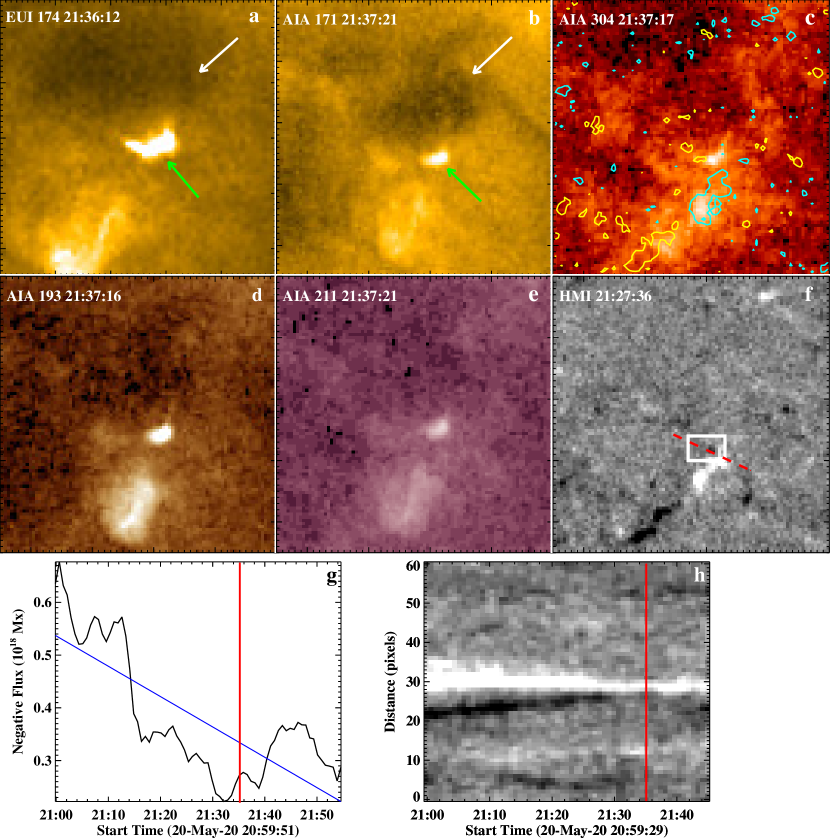
Figure 5: Campfire-8 observed on 20-May-2020 (Table 1): Panel (a) shows 174 Å HRI_EUV image of the campfire. Panels (b), (c), (d), and (e) show the AIA 171, 304, 193, and 211 Å images of the campfire, respectively. The white arrows point to the cool-plasma structure and the green arrows point to the campfire. Panel (f) shows the HMI magnetogram of the same region. The red dashed line in (f) shows cut for the time-distance map in panel (h). The white box in (f) shows the area that is used to calculate the negative magnetic flux plot shown in panel (g). Panels (g) and (h), respectively, show the negative flux plot versus time and the HMI time-distance map. The peak in (g) at 21:45 is due to flux coalescence. The rate of magnetic flux cancelation is 0.4 $\times$ 10¹⁸ mx hr^-1. The red line marks the start time of the campfire. In panel (c), HMI contours, of levels $\pm$15 G, of 21:38:06 are overlaid, where cyan and yellow contours represents the positive and negative polarities, respectively. The animation (Movie1A-AIA) runs from 21:00 to 22:08 UT and the annotations and FOV are same as in this Figure, while the EUI animation (Movie1A-So) runs from 21:32 to 21:49 UT and the animation is unannotated.

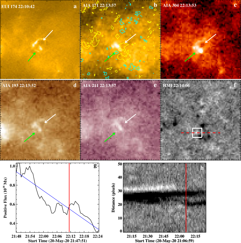
Figure 6: Campfire-13 observed on 20-May-2020 (Table 1): Panel (a) shows the 174 Å HRI_EUV image of the campfire. Panels (b), (c), (d), and (e) show the AIA 171, 304, 193, and 211 Å images of the campfire, respectively. The white arrows point to the cool-plasma structure and the green arrows point to the campfire. Panel (f) shows the HMI magnetogram of the same region. The white box in (f) shows the area that is used to calculate the positive magnetic flux plot shown in panel (g). The red dashed line in (f) shows east-west cut for the time-distance map in panel (h). Panels (g) and (h) show the positive flux plot versus time and the HMI time-distance map, respectively. Flux cancelation rate is 1.0 $\times$ 10¹⁸ mx hr^-1. The red line marks the start time of the campfire in (g) and (h). In panel (b), HMI contours, of levels $\pm$15 G, of 21:14:06 are overlaid, where cyan and yellow contours represents the positive and negative magnetic polarities, respectively. The animation (Movie2A-AIA) runs from 21:47 to 22:24 UT and the annotations and FOV are same as in this Figure, while the EUI animation (Movie2A-So) runs from 22:08 to 22:17 UT and the animation is unannotated.

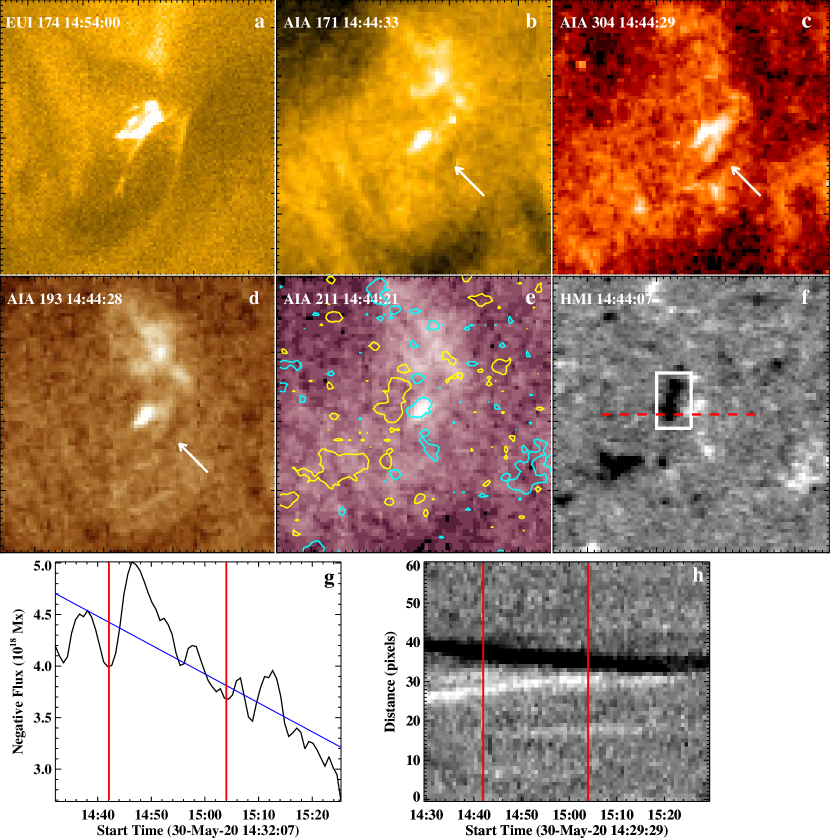
Figure 7: Campfire-22 observed on 30-May-2020 (Table 1): Panel (a) shows the 174 Å HRI_EUV image of the campfire. Panels (b), (c), (d), and (e) show the AIA 171, 304, 193, and 211 Å images of the campfire, respectively. The white arrows point to the cool-plasma structure that is accompanied by the campfire. Panel (f) shows the HMI magnetogram of the same region. The white box region in (f) shows the area that is used to calculate the negative magnetic flux plot shown in panel (g). The red dashed line in (f) shows east-west cut for the time-distance map in panel (h). Panels (g) and (h) show, respectively, the negative flux plot versus time and the HMI time-distance map along the red-dashed line in (f). The peak in Panel (g) at 14:48 is due to flux coalescence. Flux cancelation rate is 1.7 $\times$ 10¹⁸ mx hr^-1. The vertical red lines show the start time of both the campfires from the same location. In panel (e), HMI contours, of levels $\pm$15 G, of 14:44:07 are overlaid, where cyan and yellow contours represents the positive and negative magnetic polarities, respectively. This campfire is same as that shown in Figure C5/C6 in Berghmans et al. (2021). The animation (Movie3A-AIA) runs from 14:30 to 15:28 UT and the annotations and FOV are same as in this Figure, while the EUI animation (Movie3A-So) runs from 14:54 to 15:04 UT and the animation is unannotated.

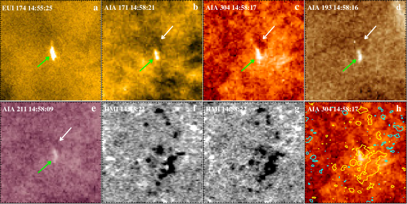
Figure 8: Campfire-23 observed on 30-May-2020 (Table 1): Panel (a) shows the 174 Å HRI_EUV image of the campfire. Panels (b), (c), (d), and (e) show the AIA 171, 304, 193, and 211 Å images of the campfire, respectively. The white arrows point to the cool-plasma structure that is accompanied by the campfire. The green arrows show the campfire. Panels (f) and (g) show the HMI magnetograms of the same region. Panel (f) shows the weak magnetic flux patches that cancel 10 min before the rise of cool plasma. In panel (e), HMI contours, of levels $\pm$15 G, of 14:58:22 are overlaid on AIA 304 Å image, where cyan and yellow contours represents the positive and negative magnetic polarities, respectively. The animation (Movie4A-AIA) runs from 14:35 to 15:09 UT and the annotations and FOV are same as in this Figure, while the EUI animation (Movie4A-So) runs from 14:54 to 15:04 UT and the animation is unannotated.

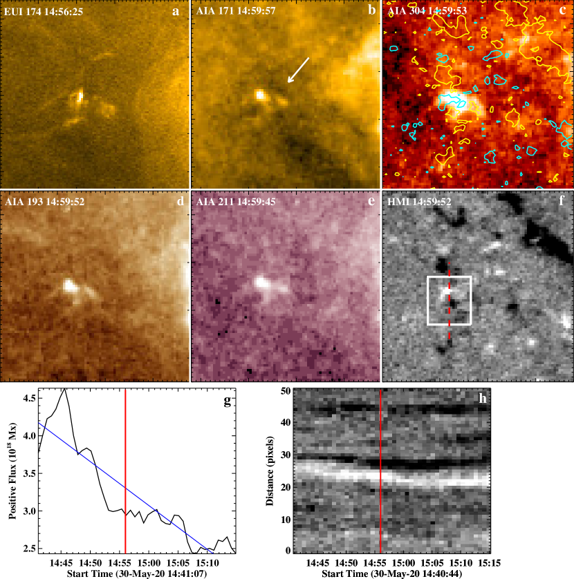
Figure 9: Campfire-25 observed on 30-May-2020 (Table 1): Panel (a) shows the 174 Å HRI_EUV image of the campfire. Panels (b), (c), (d), and (e) show the AIA 171, 304, 193, and 211 Å images of the campfire, respectively. The white arrow in (b) points to the possible structure of the cool-plasma; the cool-plasma is not visible in any other AIA channel. Panel (f) shows the HMI magnetogram of the same region. The white box in (f) shows the area that is used to calculate the positive magnetic flux plot shown in panel (g). The red dashed line in (f) shows north-south cut for the time-distance map in panel (h). Panels (g) and (h) shows the positive flux plot versus time and the HMI time-distance map. Flux cancelation rate is 3.6 $\times$ 10¹⁸ mx hr^-1. The red line marks the start time of the campfire in (g) and (h). In panel (c), HMI contours, of levels $\pm$15 G, of 14:59:52 are overlaid, where cyan and yellow contours represents the positive and negative magnetic polarities, respectively. The animation (Movie5A-AIA) runs from 14:41 to 15:17 UT and the annotations and FOV are same as in this Figure, while the EUI animation (Movie5A-So) runs from 14:54 to 15:04 UT and the animation is unannotated.

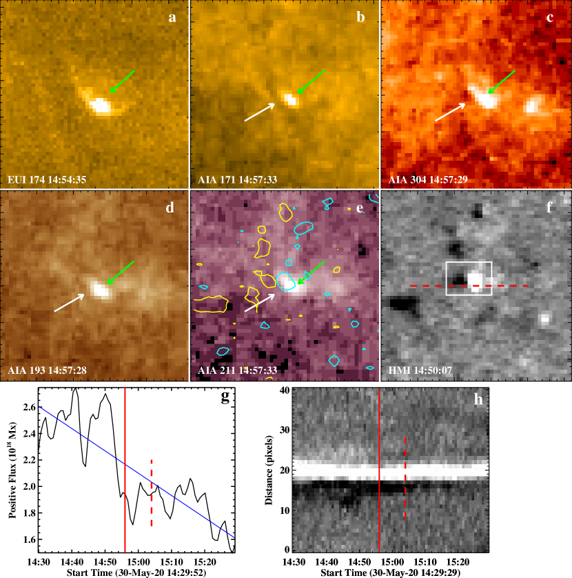
Figure 10: Campfire-26 observed on 30-May-2020 (Table 1): Panel (a) shows the 174 Å HRI_EUV images of the campfire. Panels (b), (c), (d), and (e) show the AIA 171, 304, 193, and 211 Å images of the same campfire, respectively. The white and green arrows point to the cool-plasma structure and campfire, respectively. Panel (f) shows the HMI magnetogram of the same region. The white box in (f) shows the area that is used to calculate the positive magnetic flux plot shown in panel (g). The red dashed line in (f) shows east-west cut for the time-distance map in panel (h). Panels (g) and (h) shows the positive flux plot versus time and the HMI time-distance map, respectively. Flux cancelation rate is 0.95 $\times$ 10¹⁸ mx hr^-1. The solid red lines show the peak time of the first campfire. The red-dashed lines mark the times of the second campfire that occur at the same neutral line due to ongoing flux cancelation. The blue line in (g) is the least-square fit of the flux evolution. In panel (e), HMI contours, of levels $\pm$15 G, of 14:56:52 are overlaid, where cyan and yellow contours represents the positive and negative magnetic polarities, respectively. The animation (Movie6A-AIA) runs from 14:30 to 15:29 UT and the annotations and FOV are same as in this Figure, while the EUI animation (Movie6A-So) runs from 14:54 to 15:04 UT and the animation is unannotated.

Similarly, the majority of campfires are accompanied by a cool-plasma structure (Table 1). See Section 6 for six more examples of campfires (Figures 5, 6, 7, 8, 9, and 10).

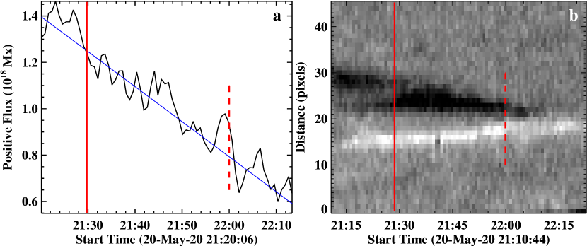
Figure 3: Magnetic field evolution at the base of the campfire presented in Figure 2. Panel (a) shows the integrated positive magnetic flux plot as a function of time computed inside the box shown in Figure 2v. Panel (b) shows the HMI time-distance maps along the red dashed lines in Figure 2u. The solid red lines show the peak time of the campfire. The red-dashed lines mark the time of the second campfire that occur at the same neutral line due to ongoing flux cancelation. The blue line is the least-square fit of the flux evolution.

3.3 Magnetic Field Evolution at Campfire’s Base

Figures 2u-x display the photospheric line of sight magnetic field at the base of the campfire. The campfire occurs at the edge of the negative-polarity magnetic flux lane (Figure 2i). In this region, the negative magnetic flux is in majority and positive flux is in minority. Both the campfire and cool-plasma reside above the same neutral line, between the majority-polarity magnetic flux patch (negative) and a merging minority-polarity flux patch (positive; Figure 2i). We followed these flux patches for about two hours and noticed that there is flux cancelation going on between positive and negative flux patch (Movie1-AIA and Figures 2u-x).

We carefully isolated the minority-polarity (positive) magnetic flux patch of the campfire-base and made a plot to show the magnetic flux evolution quantitatively (Figure 3a). The area of integrated flux is bounded by a white box in Figure 2v. Figure 3a shows that there is a decrease in the positive magnetic flux, which is due to the continuous flux cancelation between the negative flux patch and a merging positive flux patch. We interpret that the flux cancelation triggers the cool-plasma eruption and that cool-plasma drives the campfire. Another campfire appears at the same neutral line (see red-dashed line in Figure 3) apparently caused by the continuous flux cancelation. We estimate the average rate of flux decrease using the best-fit line in Figure 3a to be 1.0 $\times$ 10¹⁸ Mx hr^-1.

Figure 3b shows the time-distance map along the red-dashed line of Figure 2u. The magnetic flux patches converge and cancel, and trigger the cool-plasma eruption accompanied by the campfire. This scenario is similar to pre-jet minifilaments that are seen to form and erupt multiple times due to flux cancelation at the magnetic neutral line (Panesar et al., 2017; Sterling et al., 2017; Panesar et al., 2018a). Furthermore, the magnetic set-up of campfires are also similar to the magnetic environment of small-scale events (e.g. jetlets, explosive events, and coronal bright points) that are also seen to occur due to flux cancelation (e.g., Panesar et al., 2018b, 2019; Tiwari et al., 2019; Madjarska, 2019).

Analogous to this example, we find that all the campfires, of Table 1, reside above magnetic neutral lines and most of them are accompanied with magnetic flux cancelation (Figures 5, 6, 7, 9, and 10).

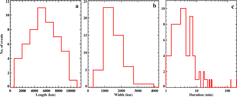
Figure 4: Histograms of the physical parameters of 52 campfires listed in Table 1. Panels (a), (b), and (c) show the histograms of the length, width, and duration of the campfires, respectively. In panel (c) the x-axis is displayed in logarithm scale. The mean (median) values of the length, width, and duration are 5400$\pm$2500 km (5500 km), 1600$\pm$640 km (1500 km), and 13.2$\pm$30 minutes (6 minutes), respectively.

3.4 DEM

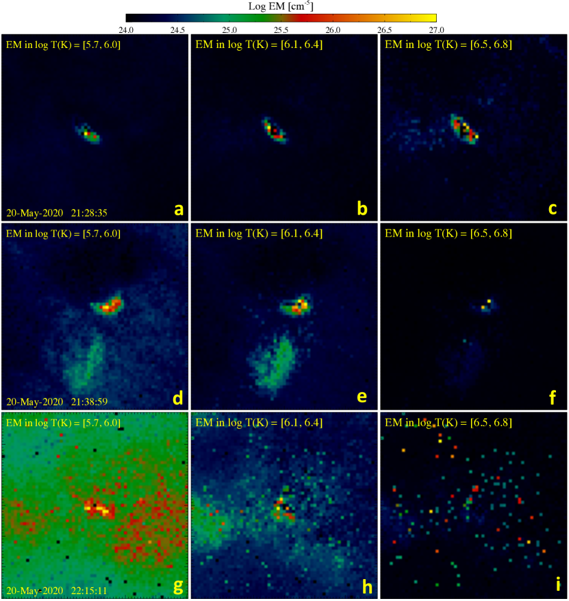
Figure 11: DEM distribution of campfires observed on 20-May-2020: Panels (a-c), (d-f), and (g-i) display the DEM maps of campfires shown in Figures 2, 5, and 6, respectively. The EM for each campfire is displayed in three different temperature bins. The color-bar on the top of the image indicates the total EM included within each log₁₀ T range mentioned in the upper left corner of each panel. The DEM maps show that these campfires have significant EM at coronal temperatures (a,b,c,d,e,g,h). However, in panels (f) and (i) there is barely any emission at temperatures above log₁₀ T(K) = 6.5.

We use images from six EUV AIA channels (171, 193, 211, 131, 335, and 94 Å) to compute the DEM distributions of our campfires. Figures 11a,b,c show the total EM of the campfire region presented in Figure 2 (campfire-2 of Table 1) that is contained within the temperature range of log₁₀ T [5.7,6.0], [6.1,6.4], and [6.5,6.8], respectively. Evidently the campfire contains high coronal temperatures. Most of the EM lies in the log₁₀ T bins of 6 to 6.6 ($\sim$ 1 to 4 MK). This particular campfire shows EM signals for low to high temperature ranges (from log T₁₀ = [5.7,6.0] to [6.5,6.8]).

Figures 11(d-f) and 11(g-i), show the DEM maps for campfires-8 and-13, from 20-May-2020. Both of these campfires are nicely visible in the temperature range of $\sim$ 0.5 to 2.5 MK but these do not show EM in 3 MK temperatures or above (in Figures 11f,i).

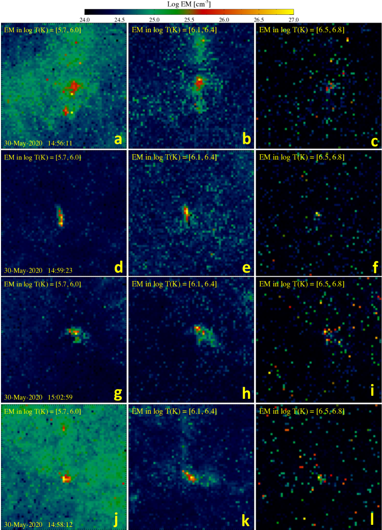
Figure 12: DEM distribution of campfires observed on 30-May-2020: Panels (a-c), (d-f), (g-i), and (j-l) show the DEM maps of campfires shown in Figures 7, 8, 9, and 10, respectively. The color-bar indicates the total EM included within a log T range shown in the upper left corner of the each panel. The DEM maps show that campfires are visible at coronal temperatures (a,b,d,e,g,h,j,k). However, in panels (c, f, i, and l) there is barely any emission at temperatures above log₁₀ T(K) = 6.5.

Similarly, Figure 12 shows the DEM distributions of campfires shown in Figures 7, 8, 9, and 10. All these campfires have large EM in the temperature range of $\sim$ 0.5 to 2.5 MK. Overall, all of these campfires appear to have emission in coronal temperatures – this is consistent with the findings of Berghmans et al. (2021).

3.5 Statistical Physical Properties

Different physical properties of 52 campfires are listed in Table 1. We find that all the campfires reside above the magnetic neutral lines. Most of the campfires (40 out of 52; exceptions are indicated in Table 1) are accompanied by a cool-plasma structure. Only in 2 events we did not find any evidence of cool-plasma – these events are relatively smaller. In 40 out of 52 events, we observe discernible flux cancelation. In a few cases, which are listed as ambiguous, campfires reside above very weak flux patches – even in those cases HMI movies show visible flux cancelation before and/or during the events. We find that in majority of events, the cool-plasma structures are formed and triggered by flux cancelation.

In Figures 4(a,b,c), we show histograms of the length, width, and duration of the 52 campfires (of Table 1), respectively. Evidently, most of the campfires have lengths between 4000 to 6000 km, but they can be as small as 750 km and as long as 10400 km. The width of the most campfires ranges between 1000 to 1600 km, but they can be as narrow as 700 km and as wide as 3800 km. The sizes of these events are evidently larger than the spatial resolution of the HRI_EUV data ($\sim$400 km). The average lengths of the campfires are smaller than the average lengths of Hi-C 2.1 jet-like events (Panesar et al., 2020a) and EUI microjets (Hou et al., 2021). The sizes of dot-like campfires are similar or smaller than the sizes of Hi-C 2.1 dot-like events (Tiwari et al., 2019). The majority of campfires (40) have durations of less than 10 minutes. But they can live as long as 198 minutes (Figure 4).

We estimated free magnetic energy (B²$\times$V/8$\pi$) of the campfires based on their sizes and approximated coronal magnetic field of 20 G, and found them to range in the order of 10²⁶ to 10²⁷ erg. For estimating the volumes of dot-like campfires, we considered spherical geometry (V=4 $\pi r^{3}$/3), and took the average of their length and width as radius r. Whereas for the loop-like, jet-like and complex campfires, we assumed a cylindrical geometry (V=$\pi r^{2}$h), and took lengths of the campfires as height h and their widths as radius r. In the absence of true measured coronal magnetic field, and due to the fact that we use the projected lengths and widths of campfires, our evaluated free magnetic energies are only crude estimates.

4 Discussion

We have examined the evolution of 52 solar campfires using HRI_EUV  images from Solar Orbiter and EUV images from SDO/AIA, and investigated their magnetic origin using line of sight magnetograms from SDO/HMI. We find that (i) all the campfires are located above magnetic neutral lines; (ii) in the majority of instances (79%), campfires are accompanied by a cool-plasma structure; (iii) 77% of campfires come from the sites of magnetic flux cancelation, analogous to coronal jets and jetlets; (iv) the cool-plasma structures are anchored at sites of flux cancelation, reminiscent of pre-jet minifilaments; (v) the campfires appear at coronal temperatures ($\sim$ 0.5 to 2.5 MK); (vi) their estimated free magnetic energies are in the order of 10²⁶ to 10²⁷ erg; and (vii) while many of the campfires are complex in their structure (previously unexplored), most of them appear as a small-scale loop, a dot, or a coronal jet. In the following we discuss our findings:

Magnetic flux cancelation: We find that all our campfires (in Table 1) are rooted at the edges of photospheric magnetic network flux lanes. Most of them occur, at neutral lines, at evident sites of magnetic flux cancelation (40 out of 52 show clear flux cancelation). In a few cases (listed as ‘ambiguous’ in the second last column of Table 1) (a) either magnetic flux cancelation occurs between the weak flux patches, or (b) the canceling minority flux is a few pixels away from the base of the campfire. However, the minority-polarity flux patches are present at or around the base of each campfire, suggestive of magnetic flux cancelation being involved in generating all campfires.

The flux cancelation rate of $\sim$10¹⁸ Mx hr^-1, at campfire’s base, are similar to the flux cancelation rates found for coronal jets in the quiet Sun regions and coronal holes (10¹⁸ Mx hr^-1; Panesar et al. (2016, 2018a)), and in large penumbral jets (10¹⁸ Mx hr^-1; Tiwari et al. (2018), but are lower than the flux cancelation rates found for active region jets (10¹⁹ Mx hr^-1; Sterling et al. (2017)), and surges in the core of active regions (10¹⁹ Mx hr^-1 ;Tiwari et al. (2019)).

Presence of cool-plasma: Most of the campfires (41 out of 52; exceptions are indicated in Table 1) are accompanied by a cool-plasma structure, which is present along the neutral line, at the base of the campfire. Only in 2 events we did not find any evidence of cool plasma. These events are relatively smaller – therefore, the cool plasma might not be discernible. Furthermore, in some cases the campfires occur multiple times from the same neutral line, similar to jets, jetlets, and network jets (Raouafi & Stenborg, 2014; Tian et al., 2014; Panesar et al., 2016, 2020b), and each time they are accompanied with a cool-plasma structure.

We infer that the presence of cool plasma structure might be an indicator of the presence of a magnetic flux rope, probably created by flux cancelation in the same way as observed for pre-jet minifilaments (Panesar et al., 2017) and for typical solar filaments (van Ballegooijen & Martens, 1989; Moore & Roumeliotis, 1992). We conjecture that the visible flux cancelation is a result of the submergence of the lower reconnected loops into the photosphere (van Ballegooijen & Martens, 1989; Priest & Syntelis, 2021; Syntelis & Priest, 2021).

Alternatively, magnetic reconnection can directly lead to generation of campfires (without flux ropes) as proposed in some analytical theories and numerical simulations for coronal jets (e.g. Yokoyama & Shibata, 1995; Shibata & Magara, 2011). This could be the case for a few campfires that do not show clear presence of a cool plasma structure marked as ‘ambiguous/no’ in the third last column of Table 1). However, there are some simulations that do show flux rope formation in coronal jets (e.g. Wyper et al., 2018; Doyle et al., 2019).

Free magnetic energy: Our estimated free magnetic energies for campfires (10²⁶ to 10²⁷ erg, as discussed earlier) are in agreement with that estimated for campfires in a numerical model by Chen et al. (2021). Our estimated free magnetic energies are also in the range of that of coronal hole jets (Pucci et al., 2013) and coronal X-ray bright points (e.g. Priest et al., 1994). The campfires’ free magnetic energies are about an order of magnitude lower in magnitude than the free magnetic energies of active region jets (Sterling et al., 2017), and of active region loops and sub-flares (Cirtain et al., 2013; Tiwari et al., 2014). Thus, campfires contain sufficient energy to heat the quiet-Sun corona, locally, which is consistent with their emission measure (EM) distributions.

Similarities with other events: Based on their appearances in HRI_EUV images, we have categorized campfires as small loop-like, dot-like, jet-like, or complex structures (as listed in Table 1). Our loop-like, jet-like/surge and dot-like events show similarities with the explosive events in the core of an active region observed by Hi-C 2.1 (Tiwari et al., 2019). The Hi-C explosive events also appeared at sites of opposite-polarity magnetic flux patches, and are confined, thus are reminiscent to campfires, albeit them being located in a different magnetic environment. The loop-like campfires also look similar to the low-lying loop nanoflare events in the moss region observed by Hi-C (Winebarger et al., 2013). The sizes of our jet-like campfires are smaller than the sizes of Hi-C 2.1 jet-like events (Panesar et al., 2019) and EUI microjets (Hou et al., 2021). Further, these two studies did not find any evidence of cool-plasma structure at the jet-base regions.

Some of the campfires might have similarities with coronal X-ray bright points – bright points are also seen to occur at the sites of magnetic flux cancelation (e.g. Longcope, 1998). However, coronal bright points might be hotter than campfires because they are visible in hotter wavelengths e.g. in X-rays (Golub et al., 1974) and/or in AIA 94 Å (Madjarska, 2019). Whereas our campfires are barely discernible in AIA 94 Å.

Small-scale transient brightenings in the quiet Sun are reportedly located in the magnetic network lanes at the boundaries of supergranule cells (Porter & Dere, 1991; Falconer et al., 1998; Gošić et al., 2014; Attie et al., 2016), similar to our findings for campfires. Some of the campfires have similar sizes and lifetimes of explosive events found in the quiet Sun regions (Dere et al., 1989). However, the explosive events in the above-mentioned study are found to have lower temperatures and thus most probably are transition region events (e.g. Chae et al., 1998; Innes & Teriaca, 2013; Gupta & Tripathi, 2015; Huang et al., 2019).

The physical properties of most campfires are in agreement with the above mentioned events (i.e., loops, dots, coronal jets and coronal bright points). Therefore the term ‘campfire’ includes different variety of small-scale solar features/events.

The presence of cool-plasma structure in most of our campfires provides evidence that tiny flux ropes are plausibly present in many of solar features, everywhere on the Sun. The magnetic flux cancelation seems to build and trigger tiny flux rope eruptions in campfires, similar to the pre-jet minifilaments (Young & Muglach, 2014; Adams et al., 2014; Panesar et al., 2016, 2017, 2018a; McGlasson et al., 2019; Muglach, 2021; Shen, 2021) and typical solar filaments (that drive CMEs e.g. Sterling et al., 2018). The only major difference lies in that the cool-plasma eruptions in jets occur along far-reaching field lines, whereas in campfires the cool-plasma eruptions are mostly confined and seem to occur at the base of closed-field lines. That is plausibly why most campfires are not seen to erupt outwards.

Our results support the simulations of campfires (Chen et al., 2021) – these are at coronal temperature and show evidence of magnetic flux ropes. However, our observations show that the presence of cool structures is much more common than inferred in the simulation (Chen et al., 2021) where only one out of the seven campfires showed a flux rope.

Our observational results provide new insights into the understanding of coronal heating by small-scale campfires, and elucidate that cool plasma structures might accompany most solar eruptions (ejective or confined). These tiny flux ropes are most probably created by small-scale magnetic flux cancelation, plausibly driven by photospheric random convective flows.

5 Conclusions

We investigate the magnetic origin of solar campfires by using Solar Orbiter/EUI and SDO (AIA and HMI) observations. Although many campfires are ‘complex’, the term campfire encompasses a wide variety of small-scale coronal events (e.g. small-scale loops, dots, and coronal jets). They occur at the edges of photospheric magnetic network flux lanes. Majority of the campfires are accompanied by a cool-plasma structure, which resides above the magnetic neutral line, where evidently magnetic flux cancelation takes place. Thus, campfires bear similarities with solar eruptions such as coronal jets and CME-producing filament eruptions. Our observations suggest that the presence of cool-plasma, i.e., magnetic flux ropes in the solar atmosphere, is more common than previously thought. The campfires contain coronal temperatures and plausibly are small-scale magnetic reconnection events.

6 Appendix information

References

- Adams et al. (2014) Adams, M., Sterling, A. C., Moore, R. L., & Gary, G. A. 2014, ApJ, 783, 11, doi: 10.1088/0004-637X/783/1/11
- Aschwanden (2004) Aschwanden, M. J. 2004, Physics of the Solar Corona. An Introduction (Praxis Publishing Ltd)
- Attie et al. (2016) Attie, R., Innes, D. E., Solanki, S. K., & Glassmeier, K. H. 2016, A&A, 596, A15, doi: 10.1051/0004-6361/201527798
- Berghmans et al. (2021) Berghmans, D., Auchère, F., Long, D. M., et al. 2021, arXiv e-prints, arXiv:2104.03382. https://arxiv.org/abs/2104.03382
- Chae et al. (1998) Chae, J., Wang, H., Lee, C.-Y., Goode, P. R., & Schühle, U. 1998, ApJ, 497, L109, doi: 10.1086/311289
- Chen et al. (2021) Chen, Y., Przybylski, D., Peter, H., et al. 2021, arXiv e-prints, arXiv:2104.10940. https://arxiv.org/abs/2104.10940
- Cheung et al. (2015) Cheung, M. C. M., De Pontieu, B., Tarbell, T. D., et al. 2015, ApJ, 801, 83, doi: 10.1088/0004-637X/801/2/83
- Cirtain et al. (2013) Cirtain, J. W., Golub, L., Winebarger, A. R., et al. 2013, Nature, 493, 501, doi: 10.1038/nature11772
- Couvidat et al. (2016) Couvidat, S., Schou, J., Hoeksema, J. T., et al. 2016, Sol. Phys., 291, 1887, doi: 10.1007/s11207-016-0957-3
- Dere et al. (1989) Dere, K. P., Bartoe, J.-D. F., Brueckner, G. E., Cook, J. W., & Socker, D. G. 1989, 119, 55, doi: 10.1007/BF00146212
- Doyle et al. (2019) Doyle, L., Wyper, P. F., Scullion, E., et al. 2019, ApJ, 887, 246, doi: 10.3847/1538-4357/ab5d39
- Falconer et al. (1998) Falconer, D. A., Moore, R. L., Porter, J. G., & Hathaway, D. H. 1998, ApJ, 501, 386, doi: 10.1086/305805
- Freeland & Handy (1998) Freeland, S. L., & Handy, B. N. 1998, Sol. Phys., 182, 497, doi: 10.1023/A:1005038224881
- Golub et al. (1974) Golub, L., Krieger, A. S., Silk, J. K., Timothy, A. F., & Vaiana, G. S. 1974, ApJ, 189, L93, doi: 10.1086/181472
- Gošić et al. (2014) Gošić, M., Bellot Rubio, L. R., Orozco Suárez, D., Katsukawa, Y., & del Toro Iniesta, J. C. 2014, ApJ, 797, 49, doi: 10.1088/0004-637X/797/1/49
- Gupta & Tripathi (2015) Gupta, G. R., & Tripathi, D. 2015, ApJ, 809, 82, doi: 10.1088/0004-637X/809/1/82
- Hou et al. (2021) Hou, Z., Tian, H., Berghmans, D., et al. 2021, ApJ, 918, L20, doi: 10.3847/2041-8213/ac1f30
- Huang et al. (2019) Huang, Z., Li, B., & Xia, L. 2019, Solar-Terrestrial Physics, 5, 58, doi: 10.12737/stp-52201909
- Innes & Teriaca (2013) Innes, D. E., & Teriaca, L. 2013, Sol. Phys., 282, 453, doi: 10.1007/s11207-012-0199-y
- Lemen et al. (2012) Lemen, J. R., Title, A. M., Akin, D. J., et al. 2012, Sol. Phys., 275, 17, doi: 10.1007/s11207-011-9776-8
- Longcope (1998) Longcope, D. W. 1998, ApJ, 507, 433, doi: 10.1086/306319
- Madjarska (2019) Madjarska, M. S. 2019, Living Reviews in Solar Physics, 16, 2, doi: 10.1007/s41116-019-0018-8
- McGlasson et al. (2019) McGlasson, R. A., Panesar, N. K., Sterling, A. C., & Moore, R. L. 2019, ApJ, 882, 16, doi: 10.3847/1538-4357/ab2fe3
- Moore & Roumeliotis (1992) Moore, R. L., & Roumeliotis, G. 1992, in Lecture Notes in Physics, Berlin Springer Verlag, Vol. 399, IAU Colloq. 133: Eruptive Solar Flares, ed. Z. Svestka, B. V. Jackson, & M. E. Machado, 69
- Muglach (2021) Muglach, K. 2021, ApJ, 909, 133, doi: 10.3847/1538-4357/abd5ad
- Müller et al. (2017) Müller, D., Nicula, B., Felix, S., et al. 2017, A&A, 606, A10, doi: 10.1051/0004-6361/201730893
- Müller et al. (2020) Müller, D., St. Cyr, O. C., Zouganelis, I., et al. 2020, A&A, 642, A1, doi: 10.1051/0004-6361/202038467
- Panesar et al. (2020a) Panesar, N. K., Moore, R. L., & Sterling, A. C. 2020a, ApJ, 894, 104, doi: 10.3847/1538-4357/ab88ce
- Panesar et al. (2017) Panesar, N. K., Sterling, A. C., & Moore, R. L. 2017, ApJ, 844, 131, doi: 10.3847/1538-4357/aa7b77
- Panesar et al. (2018a) —. 2018a, ApJ, 853, 189, doi: 10.3847/1538-4357/aaa3e9
- Panesar et al. (2016) Panesar, N. K., Sterling, A. C., Moore, R. L., & Chakrapani, P. 2016, ApJ, 832, L7, doi: 10.3847/2041-8205/832/1/L7
- Panesar et al. (2018b) Panesar, N. K., Sterling, A. C., Moore, R. L., et al. 2018b, ApJ, 868, L27, doi: 10.3847/2041-8213/aaef37
- Panesar et al. (2020b) Panesar, N. K., Tiwari, S. K., Moore, R. L., & Sterling, A. C. 2020b, ApJ, 897, L2, doi: 10.3847/2041-8213/ab9ac1
- Panesar et al. (2019) Panesar, N. K., Sterling, A. C., Moore, R. L., et al. 2019, ApJ, 887, L8, doi: 10.3847/2041-8213/ab594a
- Parker (1988) Parker, E. N. 1988, 330, 474, doi: 10.1086/166485
- Porter & Dere (1991) Porter, J. G., & Dere, K. P. 1991, ApJ, 370, 775, doi: 10.1086/169860
- Priest & Forbes (2000) Priest, E. R., & Forbes, T. G. 2000, in Magnetic reconnection : MHD theory and applications / Eric Priest
- Priest et al. (1994) Priest, E. R., Parnell, C. E., & Martin, S. F. 1994, ApJ, 427, 459, doi: 10.1086/174157
- Priest & Syntelis (2021) Priest, E. R., & Syntelis, P. 2021, A&A, 647, A31, doi: 10.1051/0004-6361/202038917
- Pucci et al. (2013) Pucci, S., Poletto, G., Sterling, A. C., & Romoli, M. 2013, ApJ, 776, 16, doi: 10.1088/0004-637X/776/1/16
- Raouafi & Stenborg (2014) Raouafi, N.-E., & Stenborg, G. 2014, ApJ, 787, 118, doi: 10.1088/0004-637X/787/2/118
- Rochus et al. (2020) Rochus, P., Auchère, F., Berghmans, D., et al. 2020, A&A, 642, A8, doi: 10.1051/0004-6361/201936663
- Scherrer et al. (2012) Scherrer, P. H., Schou, J., Bush, R. I., et al. 2012, Sol. Phys., 275, 207, doi: 10.1007/s11207-011-9834-2
- Schou et al. (2012) Schou, J., Scherrer, P. H., Bush, R. I., et al. 2012, Sol. Phys., 275, 229, doi: 10.1007/s11207-011-9842-2
- Shen (2021) Shen, Y. 2021, Proceedings of the Royal Society of London Series A, 477, 217, doi: 10.1098/rspa.2020.0217
- Shibata & Magara (2011) Shibata, K., & Magara, T. 2011, Living Reviews in Solar Physics, 8, 6, doi: 10.12942/lrsp-2011-6
- Sterling et al. (2015) Sterling, A. C., Moore, R. L., Falconer, D. A., & Adams, M. 2015, Nature, 523, 437, doi: 10.1038/nature14556
- Sterling et al. (2017) Sterling, A. C., Moore, R. L., Falconer, D. A., Panesar, N. K., & Martinez, F. 2017, ApJ, 844, 28, doi: 10.3847/1538-4357/aa7945
- Sterling et al. (2018) Sterling, A. C., Moore, R. L., & Panesar, N. K. 2018, ApJ, 864, 68, doi: 10.3847/1538-4357/aad550
- Syntelis & Priest (2021) Syntelis, P., & Priest, E. R. 2021, A&A, 649, A101, doi: 10.1051/0004-6361/202140474
- Tian et al. (2014) Tian, H., DeLuca, E. E., Cranmer, S. R., et al. 2014, Science, 346, 1255711, doi: 10.1126/science.1255711
- Tiwari et al. (2014) Tiwari, S. K., Alexander, C. E., Winebarger, A. R., & Moore, R. L. 2014, ApJ, 795, L24, doi: 10.1088/2041-8205/795/1/L24
- Tiwari et al. (2018) Tiwari, S. K., Moore, R. L., De Pontieu, B., et al. 2018, ApJ, 869, 147, doi: 10.3847/1538-4357/aaf1b8
- Tiwari et al. (2019) Tiwari, S. K., Panesar, N. K., Moore, R. L., et al. 2019, ApJ, 887, 56, doi: 10.3847/1538-4357/ab54c1
- van Ballegooijen & Martens (1989) van Ballegooijen, A. A., & Martens, P. C. H. 1989, ApJ, 343, 971, doi: 10.1086/167766
- Winebarger et al. (2013) Winebarger, A. R., Walsh, R. W., Moore, R., et al. 2013, ApJ, 771, 21, doi: 10.1088/0004-637X/771/1/21
- Wyper et al. (2018) Wyper, P. F., DeVore, C. R., & Antiochos, S. K. 2018, ApJ, 852, 98, doi: 10.3847/1538-4357/aa9ffc
- Yokoyama & Shibata (1995) Yokoyama, T., & Shibata, K. 1995, Nature, 375, 42, doi: 10.1038/375042a0
- Young & Muglach (2014) Young, P. R., & Muglach, K. 2014, Sol. Phys., 289, 3313, doi: 10.1007/s11207-014-0484-z
- Zhukov et al. (2021) Zhukov, A. N., Mierla, M., Auchère, F., et al. 2021, arXiv e-prints, arXiv:2109.02169. https://arxiv.org/abs/2109.02169