Effect of damped oscillations in the inflationary potential

Abstract

We investigate the effect of damped oscillations on a nearly flat inflationary potential and the features they produce in the power-spectrum and bi-spectrum. We compare the model with the Planck data using Plik unbinned and CamSpec clean likelihood and we are able to obtain noticeable improvement in fit compared to the power-law $\Lambda$CDM model. We are able to identify three plausible candidates each for the two likelihoods used. We find that the best-fit to Plik and CamSpec likelihoods match closely to each other. The improvement comes from various possible outliers at the intermediate to small scales. We also compute the bi-spectrum for the best-fits. At all limits, the amplitude of bi-spectrum, $f_{NL}\,$is oscillatory in nature and its peak value is determined by the amplitude and frequency of the oscillations in the potential, as expected. We find that the bi-spectrum consistency relation strictly holds at all scales in all the best-fit candidates.

1 Introduction

Over the last three decades, tremendous advances in precision cosmology have aided our understanding of the early universe. The Standard Model (SM) has emerged as the most successful model for describing the evolution of the universe owing to the support of numerous precise observations. While SM enjoys widespread acceptance, it does have a few drawbacks, such as horizon problem, flatness problem etc. Among the numerous candidate theories for the early universe, inflation Starobinsky:1979ty ; Starobinsky:1980te ; Guth ; Sato ; Mukhanov ; Linde:1981mu ; Linde has proven to be the best contender to account for these problems. Additionally, inflation has been able to account for the dynamics of primordial fluctuations that seeded the formation of large scale structures today Kolb:1990vq ; liddle_lyth_2000 . The imprints of these primordial fluctuations can be best identified in the Cosmic Microwave Background Radiation (CMB).

From COBE COBE ; COBEnormalization to the PLANCK 2020 ; planckcollaboration2020planck ; planckcollaboration2019planck mission, we have made significant progress in our understanding of CMB physics. With the help of CMB data, inflation has emerged as the most promising candidate for describing the near homogeneous and isotropic nature of the Universe over the large scale. Numerous inflationary models exist that appear to be consistent with the CMB observations, in which a near flat potential generates a nearly scale invariant spectrum of scalar perturbations. While these models appear to be consistent with the observational data, it has been noted that adding a few features to these flat power spectra may result in a better fit to the data Starobinsky:Kink ; Ivanov:1994pa ; Adams:Step0 ; Covi:Step1 ; Allahverdi:PI ; Ashoorioon:Step2 ; Joy:2007na ; Joy:2008qd ; Jain:PI ; Pahud:Osc2 ; Hazra:Step3 ; McAllister:Osc0 ; Flauger:Osc1 ; Miranda:Step4 ; Aich:Osc3 ; Peiris:Osc4 ; Benetti:Step5 ; Meerburg:Osc5 ; Easther:Osc6 ; Bousso:Step8 ; GallegoCadavid:Step6 ; Chluba:Step7 ; Motohashi:Osc7 ; Miranda:Osc8 . These additional features are found to fit a few consistent outliers that are being observed in the data for decades Hannestad_2001 ; Tegmark_2002 ; Shafieloo_2004 ; Hazra_2013 ; Nicholson_2009 ; Nicholson_2010 ; SL_Bridle ; Shafieloo_2007 ; Shafieloo_2008 ; Hazra:recon13broad ; Hazra:reconP13 ; Hunt:2015iua ; Obied:2018qdr ; Braglia:2020fms ; Braglia:2021ckn ; Hazra:2021eqk ; Braglia:2021rej ; Braglia:2021sun . The persistent existence of these outliers could be owing to some unknown features of inflationary dynamics, which could expand our understanding of the early universe. As a result, it is critical to investigate about these features in the power spectrum. We provide a single field canonical inflationary potential in this study that simulates these extra features using damped sinusoidal oscillations. A noteworthy aspect of this feature is that it could generate both sharp and resonant featured oscillations, as well as their combinations Chen:2016zuu . Primordial standard clock Chen:2014cwa is one model that can generate a combination of sharp and resonant spectral features, but it is a two field inflationary model. It is shown in Antony:2022ert that these features could account for the additional smoothing in the CMB temperature spectrum, thus resolving the $A_{lens}$ anomaly. It increases $H_{0}$ while decreasing $S_{8}$. Additionally, the model fits the One spectrum Hazra:2022rdl , which resolves many tensions and anomalies in the Planck data. In this study, we examine alternative best fit candidates for this feature, in addition to the one mentioned in Antony:2022ert , by analysing the entire $k$-space. Using Planck CMB data, we identify these features in the primordial power spectrum using this range of spectra. Later, we will demonstrate that these features could account for some of the in outliers CMB data that are not captured by the power-law form of the primordial power-spectrum. We examine a few possible candidates, sharp featured and resonant featured, that improve the fit to CMB data noticeably.

This paper is structured as follows. In section 2, we introduce the potential form and discuss the methodology of work as well as the various datasets used for it. The results and discussion of various best-fit candidates are provided in section 3. Finally, we discuss the conclusions and inferences drawn from the work in section 4. Appendices contain the analytical calculations used in the work. We used natural units throughout the paper, $\hbar=c=M_{pl}=1$. In this paper, we use the metric signature (-,+,+,+). For formalising the equations, we used three sets of coordinates for time, namely cosmic time $(t)$, conformal time $(\eta)$, and the number of e-folds $({\mathcal{N}})$. We work in an expanding homogeneous and isotropic universe whose metric is given by the Friedmann Lemaitre Robertson Walker (FLRW) metric having perturbations up to linear order. An over-dot and an over-prime denote differentiation in terms of $t$ and $\eta$, respectively. Differentiation with respect to ${\mathcal{N}}$ is given by a subscript ${\mathcal{N}}$, i.e. $f_{{\mathcal{N}}}=\mathrm{d}f/\mathrm{d}{\mathcal{N}}$.

2 Model and data

In this paper, we investigate the dynamics of a single canonical scalar field in an inflationary potential. Our potential is divided into two parts: a baseline with a slow roll regime where we could begin the inflation, and a small feature in the form of damped cosine oscillation. The nearly scale invariant (slightly red titled) power-spectrum is obtained from the baseline part of the potential. We add features in this baseline potential to capture extra possible signals in CMB data. The feature we propose could be added to any baseline potential that could produce a near scale invariant power spectrum. This was verified using a couple of different base potentials. One can also directly add features to the power-spectrum and estimate parameters, but in such cases, it may be difficult to obtain an expression for potential back from the spectra. Therefore, we work with features in the potential itself.

We consider the potential to be of the following form,

$${V(\phi)=\gamma^{2}\phi\cosh{(\beta_{1}\phi)}+\frac{\alpha\cos{(\omega_{\phi}\phi)}}{[\beta_{2}(\phi-\phi_{0})]^{2}+C}.}$$ (1)

Here $\beta_{1}$ and $\beta_{2}$ are fixed and $C$ is an arbitrary constant added to avoid the divergence at $\phi=\phi_{0}$. It can be any value other than $0$. The power-spectrum tilt is controlled by $\beta_{1}$. We fix $\beta_{1}$ by performing a parameter estimation with only baseline potential parameters, i.e. by varying only two parameters $\gamma$ and $\beta_{1}$. We allow $\beta_{1}$ to vary between values that result in an approximate tilt of $0.94-0.98$. This analysis done using Plik bin1. The best-fitting value for $\beta_{1}$ results in a tilt of $\sim 0.96$. $\beta_{2}$ regulates the amount of damping applied to the oscillations, ensuring that features remain localised. We can see from Figure 1 that using the above potential, we can produce both sharp ($\omega_{\phi}\rightarrow 0$) and resonant features ($\beta_{2}\rightarrow 0$)in the power-spectrum.

Figure 1: This figure shows two types of features that can be generated by our model in different limits. Here, the red curve is the sharp featured oscillation whose peaks are separated linearly in k and purple curve corresponds to the resonant features whose peaks are separated uniformly in $\log k$. Note that the x-axis is in $\log$ scale here.

We vary four parameters in the full potential function, one in the baseline part and three in the feature part. The effect of each parameter on the power-spectrum could be understood from Figure 2.

Figure 2: Variation of the power spectrum in response to changes in potential parameters. Here, we varied one parameter by a specific step size while holding the other three constant. In the upper right corner of each panel, the varying parameter is specified.

Potential, as described in Equation 1, contains sinusoidal oscillations which damps as we move both sides from $\phi_{0}$. Assuming a slow roll dynamics during the initial phase of inflation, given an initial value for the field($\phi_{i}$), one can obtain other initial conditions required to calculate the background dynamics. Here we are working with number of e-folds (${\mathcal{N}}$), defined as $a=a_{i}\mathrm{e}^{\mathcal{N}}$ where $a$ is the scale factor. Initially, the potential term dominates the kinetic term therefore one can approximate Hubble parameter as, $3H^{2}\approx V(\phi)$. Therefore, $(\phi_{\mathcal{N}})_{i}$ for a given $\phi_{i}$ evaluates to be,

$$H_{i}=\sqrt{V(\phi_{i})/3},$$ (2a)

$${\phi_{\mathcal{N}}}_{i}=-\frac{V_{\phi}(\phi_{i})}{3H_{i}}.$$ (2b)

Once we have the initial conditions we solve for the background equations and get the form of $\phi$, $\phi_{\mathcal{N}}$, and $H$ as a function of e-folds(${\mathcal{N}}$). We do all these calculations using the FLRW metric. With aforementioned quantities, we can get the slow roll parameter, $\epsilon({\mathcal{N}})$, and calculate the end of inflation($\epsilon({\mathcal{N}}_{end})=1$). To find initial value of scale parameter, $a_{i}$, we impose that the mode $k=0.05~{}{\rm Mpc^{-1}}$ crosses the horizon at ${\mathcal{N}}={\mathcal{N}}_{end}-50$ Hamann:2007pa . Once the background is evaluated completely, we add the perturbations to the fields and solve for the curvature perturbation as discussed in Appendix A

The field continues to be in the slow roll phase till it feels the effect of oscillations. Once the effect of oscillations take over, the field accelerates into an intermediate fast-roll phase which is responsible for the features in power-spectrum. Inflation continues as the field rolls further down the potential till $\epsilon$ becomes one. Assuming Bunch-Davies initial condition Bunch-Davies , one solves for the curvature perturbation (${\mathcal{R}}$),

$${\mathcal{R}}_{k}^{\prime\prime}+2\bigg{(}\frac{z^{\prime}}{z}\bigg{)}{\mathcal{R}}_{k}^{\prime}+k^{2}{\mathcal{R}}_{k}=0,$$ (3)

and get the power-spectrum from

$${\mathcal{P}}_{s}(k)=\frac{k^{3}}{2\pi^{2}}\mathinner{\!\left\lvert{\mathcal{R}}_{k}\right\rvert}^{2}.$$ (4)

One can also use the Mukhanov-Sasaki equation (Equation 13) to get the power-spectrum.

We calculate the primordial power-spectrum numerically with the help of publicly available code BINGO Hazra_2013_BINGO . BINGO solves for ${\mathcal{R}}$ for each $k$ to get ${\mathcal{P}}_{s}$ as a function of $k$. Technically, one needs to integrate curvature perturbation throughout the inflationary epoch. But it can be safely approximated to a region from ${\mathcal{N}}_{i}$ deep inside Hubble radius($k\gg aH$) and to an ${\mathcal{N}}_{e}$ well outside the Hubble radius($k\ll aH$). This could be calculated using the following conditions:

$$k= {C}_{IC}a({\mathcal{N}}_{i})H({\mathcal{N}}_{i}),$$ (5a)

$$k= {C}_{SHS}a({\mathcal{N}}_{e})H({\mathcal{N}}_{e}).$$ (5b)

For each mode, we calculate the ${\mathcal{N}}_{i}$ and ${\mathcal{N}}_{e}$ using appropriate choice of ${C}_{IC}$ and ${C}_{SHS}$ values Salopek:1988qh . We fix $C_{SHS}$ but we do vary $C_{IC}$ depending on the oscillations present at a given scale, i.e. for modes near high frequency oscillations in power-spectrum, we use a larger value for $C_{IC}$. Typically, it’s value is 200.

We incorporate BINGO into CAMB Lewis_2000 ; CAMB and calculate the angular power-spectrum using the Boltzmann equations. We run Markov Chain Monte Carlo (MCMC) using CosmoMC Lewis_2002 ; COSMOMC and identify regions in parameter space which gives an improvement in fit. Starting from the aforementioned regions, we then run BOBYQA BOBYQA to obtain the best-fit values for the parameters.

We performed our analysis using the Planck mission’s most recent CMB temperature and polarisation anisotropy data. Planck was able to map the CMB sky over a wide range of multipoles ($\ell=2-2500$) on both small ($\ell\geq 30$) and large ($\ell=2-29)$ scales. We use two sets of likelihood for high-$\ell$ in our analysis: Plik-bin1-TTTEEE Planck:2019nip ; 2020 and CamSpec-v12-5-HM-cln-TTTEEE efstathiou2020detailed . We use commander-dx12-v3-2-29 for low-$\ell$ TT and simall-100x143-offlike5-EE-Aplanck-B for low-$\ell$ EE. Plik-bin1-TTTEEE represents the completely unbinned TTTEEE likelihood, and CamSpec represents the newly cleaned CamSpec. CamSpec-v12-5-HM-cln-TTTEEE employs a sophisticated data analysis pipeline to generate an improved CamSpec likelihood and also an increased sky fraction for temperature and polarisation. In our study, we vary the nuisance parameters in addition to the background parameters, and we include the priors involved, as indicated in the Planck 2018 and CamSpec likelihood papers 2020 ; efstathiou2020detailed . The prior used for the potential parameters is given in Table 1. We perform the analysis across multiple parameter templates and narrow it down to three best-fit candidates for each likelihood. The following section will discuss these three candidates in greater detail.

Parameters Prior

$$\gamma(\times 10^{4})$$ 0.14 - 0.20

-2.0 - 2.0

12.9 - 13.9

0 - 529

Table 1: The table contains the prior range we used for the inflationary potential parameters

CamSpec-v12-5-HM-cln-TTTEEE
Low-T (commander-dx12-v3-2-29)
Low-E (simall-100x143-offlike5-EE-Aplanck-B) CamSpec clean(CS)

Plik-bin1-TTTEEE
Low-T (commander-dx12-v3-2-29)
Low-E (simall-100x143-offlike5-EE-Aplanck-B) Plik-bin1(Plik)

Table 2: Short hands used for the combination of Planck likelihoods used for the analysis. We have used same low $\ell$ (lowT+lowE) likelihoods for both the sets.

3 Results

The following is the nomenclature used to identify the candidates: The likelihood against which it is tested followed by the candidate number. For example, Plik-1 specifies that it’s the first candidate analysed against Plik likelihood.

3.1 Best-fit Candidates

We explored the parameter space using MCMC algorithm and were able to identify multiple regions that could improve the fit to data (Figure 3). We perform the analysis using Plik-bin1. To identify these regions, we study various points that lie within $\Delta\chi^{2}=1$ region from the global minima of $\chi^{2}$ value of the MCMC run using BOBYQA. While performing the BOBYQA analysis we make use of both Plik-bin1 and CamSpec clean likelihoods. Using BOBYQA analysis, we are able to identify three candidates that gave improvement in fit for each likelihood. Those are Plik-1, Plik-2, Plik-3 (Plik  candidates) and CS-1, CS-2, CS-3 (CS  candidates). We also calculated the bayesian evidence using MCEvidence2017arXiv170403472H python package. The evidence only provided a 0.3-factor weak support for the baseline model. But according to Jeffrey’s scale, this is an inconclusive evidence.

Figure 3: The figure contains the triangle plot for the feature model parameters corresponding to Plik bin1. Here we can see multiple region in parameter space which could lead improved fit to data using different combination of these parameters.

The best-fit values for the Plik runs are presented in Table 3. We investigated three candidates for the Plik-runs based on the $\chi^{2}$ improvement we obtained from the BOBYQA runs. We are comparing it to the $\chi^{2}$ obtained from the power-law form of the primordial spectrum (referred to as the power-law model from now on), which has a $\chi^{2}=24548.5$ value. We can see from Table 3 that we get 10, 8.5, and 6 improvement for the candidates Plik-1, Plik-2, and Plik-3, respectively. The residual plot from Plik-runs with respect to the power-law model is shown in Figure 4. The power-law model is represented by the zero line, and the coloured lines are candidates. We can observe slight power suppression in the case of Plik-3. Here the improvement comes mainly from the high-$\ell$,  4.3 while the low $\ell$ gives around 1.45 improvement. Plik-3 also gave 2. The TT residual plot is able to capture the outliers in the range $\ell=1000-1500$, while the EE and TE residuals could capture comparatively lower multipoles ranging from 140 to 600. The exact outlying multipole values captured by the Plik-candidates are given by the Table 5.

Parameters Plik-1 Plik-2 Plik-3

$$\Omega_{b}h^{2}$$ 0.0223 0.0223 0.0222

0.1200 0.1204 0.1207

1.0409 1.0408 1.0409

0.0560 0.0585 0.0510

0.1724 0.1729 0.1716

-0.1271 0.6378 -1.223

12.97 12.99 13.20

286.96 3.13 132.02

24538.47 24539.98 24542.57

Table 3: Best-fit parameters and likelihood obtained for the candidates of the Plik-bin1 TTTEEE+lowT+lowE likelihood. First four are the $\Lambda$CDM background parameters and the next four are the inflationary potential parameters. Final row gives the $\chi^{2}$ values obtained by the candidates. Improvement in fit obtained are 10, 8.5, and 6 respectively for the candidates Plik-1, Plik-2, and Plik-3.

Figure 4: Residual plots corresponding best-fit candidates to Plik-bin1 TTTEEE+lowT+lowE likelihood. Here residual is calculated from the power-law $\Lambda$CDM model. Zero line corresponds to the power-law $\Lambda$CDM model and data points are from the 2018 Planck Plik data residual to the power law best fit.

The best-fit values for the CS runs are given in Table 4. The $\chi^{2}$ value for power-law primordial power-spectrum is $10211.3$, i.e. the improvement for candidates CS-1, CS-2, CS-3 are $5.0,3.8$ and $3.7$ respectively. Figure 5 contains the residual plots for CS runs with respective to the power-law model. Similar to Plik-candidates, residual plot of CS candidates for TT also captures the outliers in large $\ell$ values and EE captures for $\ell\sim 400$. The complete list $\ell$ values of the outliers captured by the CS candidates are given in Table 5.

Parameters CS-1 CS-2 CS-3

$$\Omega_{b}h^{2}$$ 0.0222 0.0222 0.0221

0.1205 0.1200 0.1208

1.0406 1.0410 1.0409

0.0545 0.0602 0.0524

0.1723 0.1728 0.1717

-0.1021 0.6394 -1.224

12.97 12.99 13.21

294.8 4.05 132.25

10206.29 10207.51 10207.55

Table 4: Best-fit parameters and likelihoods obtained for the candidates of the CamSpec clean TTTEEE+lowT+lowE likelihood. First four are the $\Lambda$CDM background parameters and the next four are the inflationary potential parameters. Final row gives the $\chi^{2}$ values obtained by the candidates. Improvement in fit obtained are 5, 3.8, and 3.7 respectively for the candidates CS-1, CS-2 and CS-3.

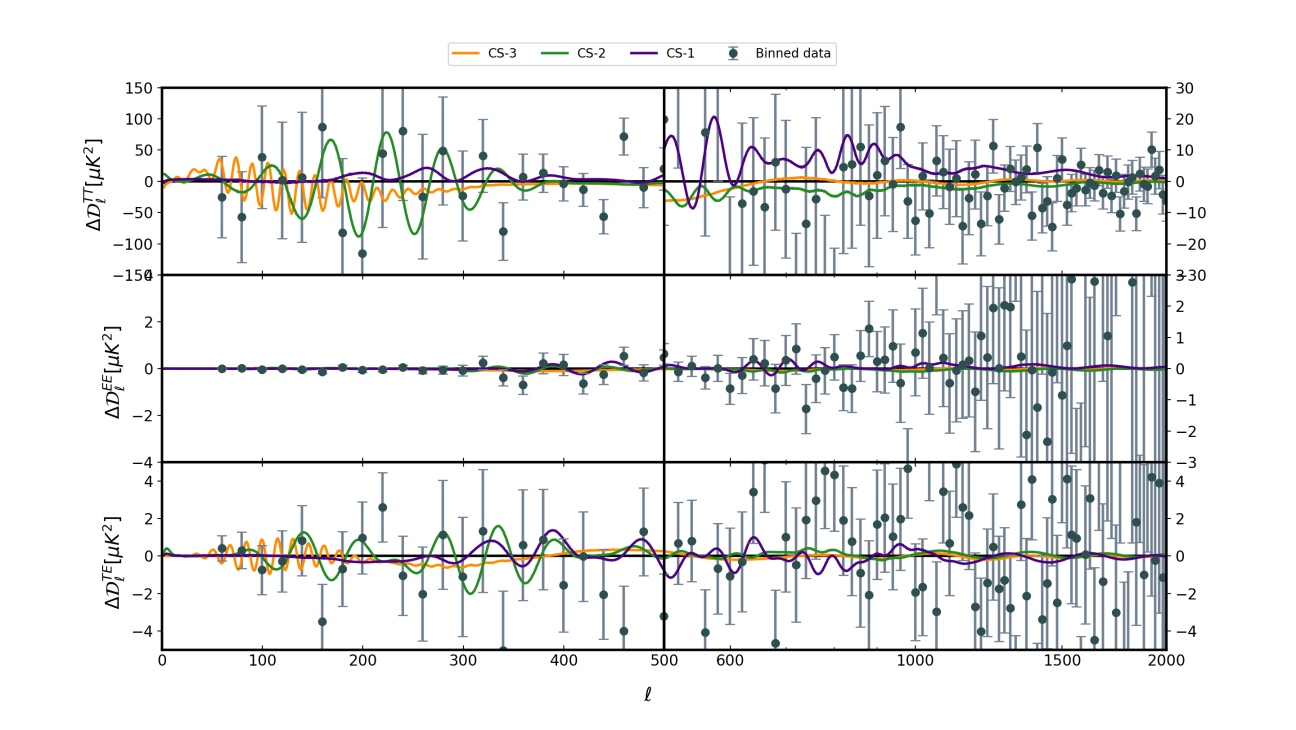
Figure 5: Residual plots corresponding best-fit candidates to CamSpec clean TTTEEE+lowT+lowE likelihood. Here residual is calculated from the power-law $\Lambda$CDM model. Zero line corresponds to the power-law $\Lambda$CDM model and data points are from the 2018 Planck CamSpec data residual to the power law best fit.

RUNS	TT	EE	TE
Plik-1	500, 520	60, 420, 440	500
Plik-2	500,1080,1340,1580	60, 140, 440	160, 200,240,260,500
Plik-3	1080, 1340	60	240
CS-1	520, 960, 1240, 1400	420	640
CS-2	1000, 1140,1420,1520	420	-
CS-3	-	340	-

Table 5: Outliers addressed by the Plik-bin1 (first three) and CamSpec clean (last three) candidates from the residual plots of TT, EE and TE correlation in Figure 4 and Figure 5.

3.2 Scalar power-spectrum

We present here the local and global best-fits to the data. We saw an improvement in $\chi^{2}$ at three different points in the parameter space. One for low frequency, one for intermediate frequency, and one for high frequency oscillations. CS-1 and Plik-1, which have a high frequency, are the global best-fit to the data for both CamSpec clean and Plik-bin1 likelihoods. They are both located in very close proximity in the parameter space. Plik-1, the best-fitting Plik candidate, has features at a smaller scale, $k\sim 4\times 10^{-2}~{}{\rm Mpc^{-1}}$, whereas Plik-3 has the features at slightly larger scales that end near $k\sim 10^{-2}~{}{\rm Mpc^{-1}}$. Plik-2 have features ranging from $k\sim 10^{-3}~{}{\rm Mpc^{-1}}$ to $k\sim 5\times 10^{-2}~{}{\rm Mpc^{-1}}$. We saw a similar pattern with the CamSpec clean candidates, which are very close to the Plik candidates in the parameter space and in the same order. The power-spectrum for both sets of candidates has been plotted in Figure 6 and Figure 7. In Figure 8, a comparison of the global best-fit for two sets of candidates is given. Both are found in the same location, and the amplitude and frequency of the oscillations are comparable.

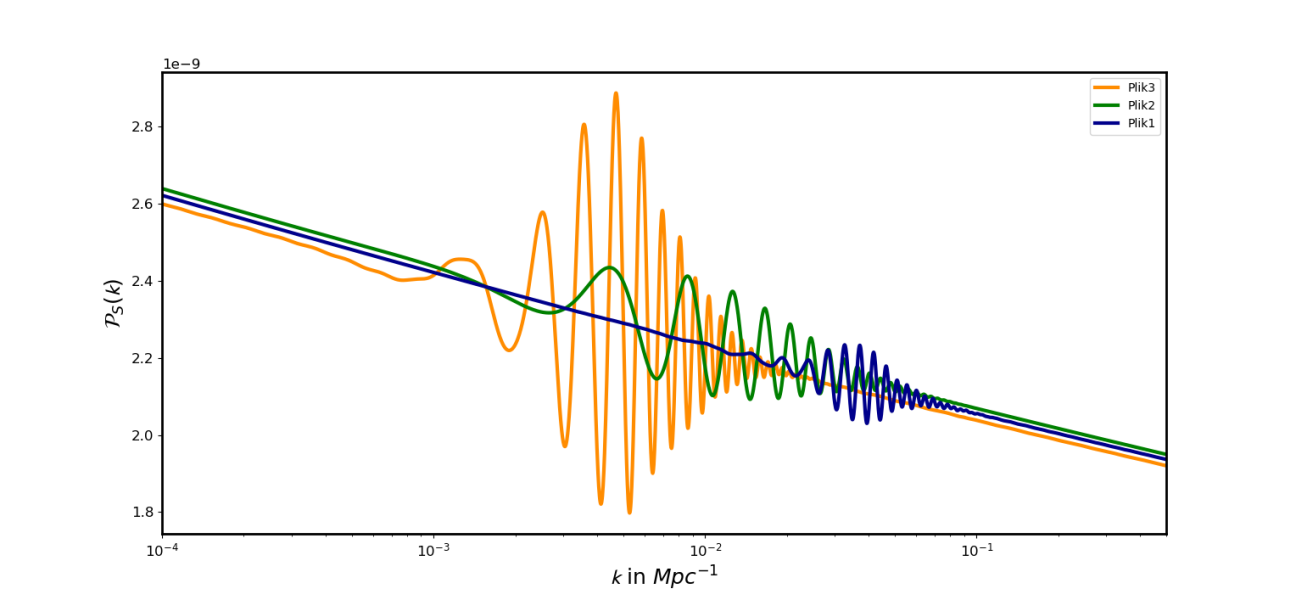
Figure 6: power-spectrum for the best-fit candidates to the Plik-bin1 likelihood Plik-1, Plik-2 and Plik-3.

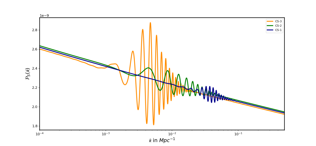
Figure 7: power-spectrum for the best-fit candidates to the CamSpec clean likelihood CS-1, CS-2 and CS-3.

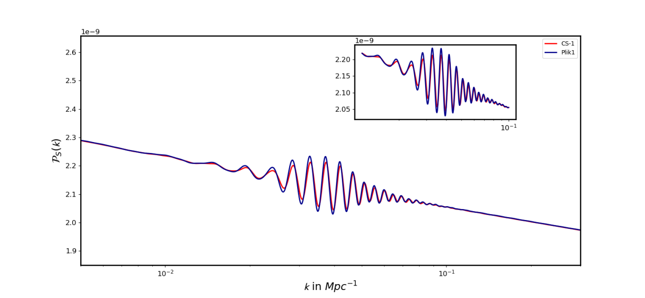
Figure 8: power-spectrum for the global best-fit of both CamSpec clean (CS-1) and Plik-bin1 (Plik-1) likelihood.

3.3 Scalar bi-spectrum

Non-Gaussianity in canonical inflationary models that are completely governed by slow roll dynamics is negligible Maldacena_2003 ; Seery:2005wm . Deviations from the slow roll nature, on the other hand, produce scale dependent oscillations in the $f_{NL}(k)$ Chen_2008 ; Chen:Osc00 ; Chen:2010xka ; Flauger:2010Osc ; Chen:2010Osc ; Martin:2011sn ; Hazra_2013_BINGO ; Hazra:2012kq ; planck2013_NG ; Adshead:2013zfa ; Achucarro:2013cva ; planck2015_NG ; Sreenath_2015 ; Martin:2014kja ; Achucarro:2014msa ; Fergusson:2014hya ; Meerburg:2015owa ; Appleby:2015bpw ; Dias:2016rjq ; planckcollaboration2019planck . As a result, features in our candidates produce a significant oscillatory bi-spectrum. In this section, we compute the $f_{NL}$ for each of the six candidates. We are evaluating bi-spectrum in three limits: equilateral ($k_{1}=k_{2}=k_{3}$), squeezed ($k_{1}\approx k_{2}\gg k_{3}$), and scalene (arbitrary triangular configuration). In all three limits, we use BINGO to evaluate the $f_{NL}$. To calculate the $f_{NL}$, we use the same method described in subsection 3.2 and substitute in Appendix C. Figure 9 displays the $f_{NL}$ for all six candidates in the equilateral limits. One can show that in the squeezed limit $f_{NL}$ reduces to

$$f_{NL}=\frac{5}{12}\left(n_{s}-1\right).$$ (6)

This relation is called the consistency condition Maldacena_2003 ; Creminelli . Figure 10 verifies the consistency relation for all six candidates. The numerically calculated $f_{NL}$ matches well with the analytical result. In the scalene limit, we obtain the 2D heat map of $f_{NL}(k_{1}/k_{3},k_{2}/k_{3})$ by fixing the value of $k_{3}$ Hazra_2013_BINGO . Figure 11 plots the 2D heat map of $f_{NL}$. Top left corner of 2D map can be identified as the squeezed limit, i.e. $k_{2}=k_{3}\gg k_{1}$ and the top right corner is the equilateral limit, i.e. $k_{1}=k_{2}=k_{3}$.

One can locate the maximum non-Gaussianity of three point correlation in equilateral limits (Figure 9). Here, CS-2 and Plik-2 generates a $f_{NL}\,$$\sim 6$. This is because of the low frequency oscillations present in the potential and thereby in the scalar power-spectrum. CS-3 and Plik-3 generates highest $f_{NL}\,$ amongst these candidates which is around $\sim 33$. This is due to the presence high amplitude and relatively larger frequency of oscillations present in the potential. Even though Plik-1 and CS-1 have large frequency oscillations, their amplitude is small compared to other four candidates which results in a $f_{NL}\,$$\sim 19,15$ respectively.

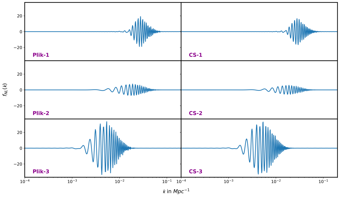
Figure 9: Scalar bi-spectrum evaluated in the equilateral limit for the best-fit candidates of the both Plik-bin1 (left side) CamSpec clean (right side) likelihood.

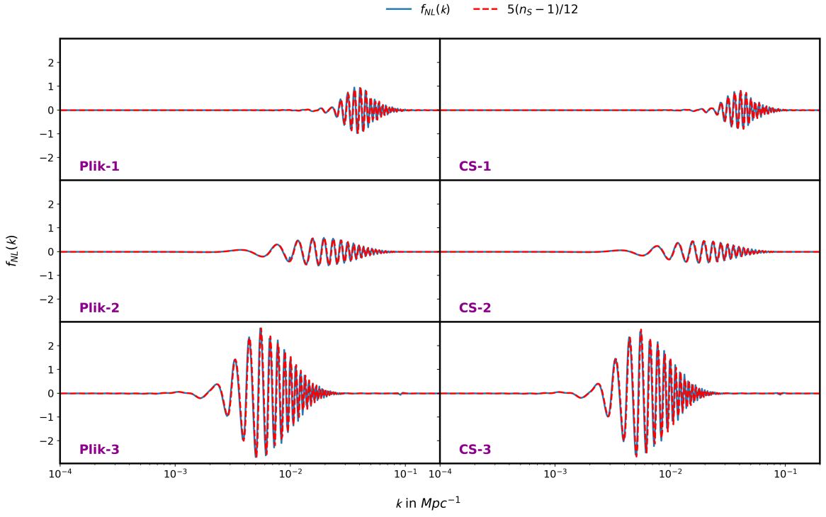
Figure 10: Verifying consistency relation (Equation 6) for the best-fit candidates to the Plik-bin1 (left side) and CamSpec clean (right side) likelihood.

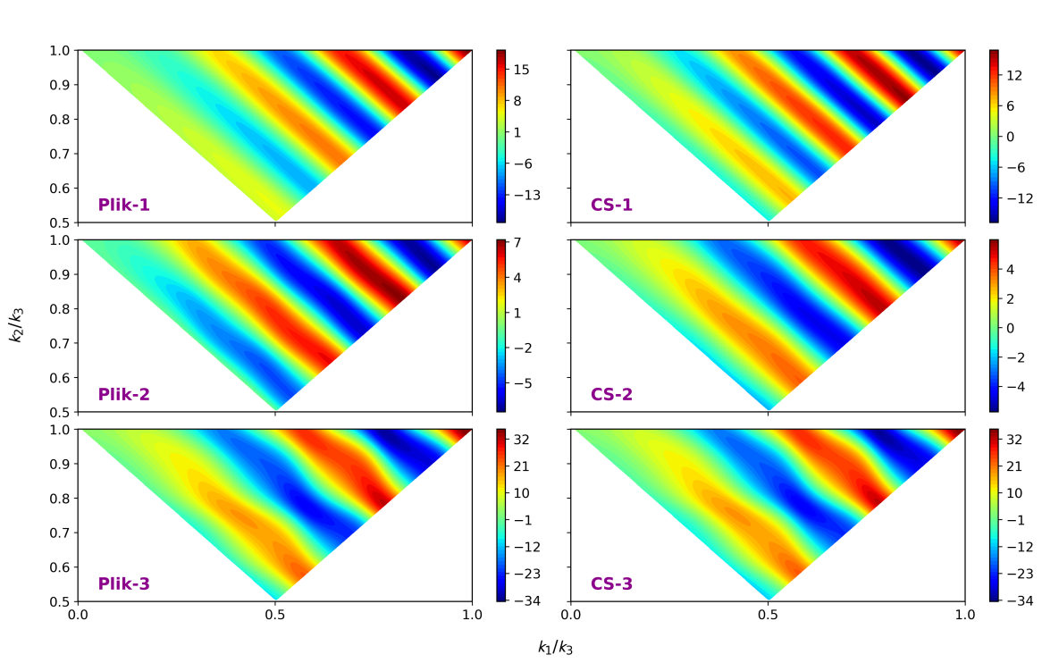
Figure 11: 2D heat map of $f_{NL}(k_{1}/k_{3},k_{2}/k_{3})$ for the best-fit candidates to the Plik-bin1 (left side) and CamSpec clean (right side) likelihood. $f_{NL}$ values are given in the color bar. Here $k_{3}$ is the mode which gave the maximum $f_{NL}$ in the equilateral limit for the corresponding candidate.

4 Conclusion

We have studied the effect of damped oscillations in a nearly flat inflationary potential and compared the spectra with Planck 2018 data. Our model is able to identify resonant features and sharp feature separately at different scales. We are able see that at smaller scales data prefers resonant features but at the intermediate scales sharp oscillations give better fit. We have separately used two high $\ell$ likelihoods, namely Plik-bin1 and CamSpec clean, for the analysis. With the addition of 3 parameters, we are able to get around $10$ and $5$ improvements for Plik-bin1 and CamSpec clean likelihood respectively. The Bayesian analysis didn’t give any conclusive evidence for the model. We have studied three candidates each for both Plik-bin1 and CamSpec clean likelihoods. They have provided $10,8.5,6$ improvements for the Plik-bin1 and $5,3.8,3.7$ for the CamSpec clean. This indicates that the extent of improvement is less in the CamSpec clean compared to the Plik-bin1 for all candidates. While the first candidate has features located at the smaller scales ($10^{-2}-10^{-1}~{}{\rm Mpc^{-1}}$), the third one has oscillations at large to intermediate scales ($10^{-3}-10^{-2}~{}{\rm Mpc^{-1}}$). The second candidate has features at the intermediate to small scales. Owing to the feature location for different candidates, different outliers are captured in the $\ell$ space. Scalar bi-spectrum, $f_{NL}\,$, is evaluated in the squeezed, equilateral limits and also in the scalene configurations. All candidates provide oscillating $f_{NL}\,$with the maximum amplitude reaching up to 33. The first and third candidate have produced relatively higher $f_{NL}\,$amplitude, $\sim 17,33$, while the second one have generated a maximum $f_{NL}\,$of $\sim 6$ in the equilateral limit. In squeezed limits, the consistency condition is satisfied at all scales for all three candidates of both likelihoods. Along with the constraints on $f_{NL}\,$, we can further narrow down the possible candidates for inflation in future. The feature candidates have overlap with scales that future Large Scale Structure (LSS) probes Euclid ; LSST ; Hazra:2012LSS ; Chen:2016LSS ; Ballardini:2016LSS ; LHuillier:2017lgm ; Beutler:2019LSS ; Ballardini:2019LSS ; Debono20 can explore. Therefore, a joint analysis can help in understanding the significance of these features better.

Appendix A Theory of inflation

One could engineer an accelerated expansion of the universe very shortly after big-bang with the help of a single canonical scalar field called inflaton, $\phi(t)$, moving in a potential $V(\phi)$. The action governing such a scalar field is given by

$${\mathcal{S}}[\phi]=\int\mathrm{d}^{4}x\sqrt{-g}\big{[}X-V(\phi)\big{]},$$ (7)

where $X=-\frac{1}{2}\nabla^{\mu}\phi\nabla_{\mu}\phi$.

Apart from a few simple potential forms, it is not easy to solve the Einstein’s equations analytically. In such situations, one can resort to numerical methodologies. For numerical analysis, a better choice of coordinate will be the number of e-folds denoted by ${\mathcal{N}}$. It tells number of e-fold times universe expanded in a given cosmic time, i.e. $a=a_{i}\mathrm{e}^{\mathcal{N}}$. The relation between $t$ and ${\mathcal{N}}$ is given by

$$d{\mathcal{N}}=Hdt,$$ (8)

where $H$ is the Hubble’s parameter in $t$. Evaluating the Einstein’s equation corresponding to the FLRW universe (also called Friedmann equations) and the equation of motion of the field, we get

$$H^{2}= \frac{V(\phi)}{3-\phi_{\mathcal{N}}^{2}/2},$$ (9a)

$$\frac{H_{\mathcal{N}}}{H}= -\frac{\phi_{\mathcal{N}}^{2}}{2},$$ (9b)

$$\phi_{{\mathcal{NN}}}+\phi_{\mathcal{N}}\Big{(}3+\frac{H_{\mathcal{N}}}{H}\Big{)}+\frac{V_{\phi}}{H^{2}}=0,$$ (10)

where subscript $\phi$ denotes the differentiation with respect to $\phi$.

With the help of background equations and linear perturbation theory (Appendix B), we get the governing equation for the curvature perturbation modes as,

$${\mathcal{R}}_{k}^{\prime\prime}+2\bigg{(}\frac{z^{\prime}}{z}\bigg{)}{\mathcal{R}}_{k}^{\prime}+k^{2}{\mathcal{R}}_{k}=0,$$ (11)

where $z=a\phi^{\prime}/{\mathcal{H}}$. ${\mathcal{H}}$ is the Hubble parameter in $\eta$ coordinate. Substituting ${\mathcal{V}}={\mathcal{R}}z$ Sasaki:1986hm ; Mukhanov:1987pv ; MUKHANOV1992203 ; Stewart_1993 one can obtain the Mukhanov-Sasaki equation.

$${\mathcal{V}}_{k}^{\prime\prime}+\bigg{[}k^{2}-\Big{(}\frac{z^{\prime\prime}}{z}\Big{)}\bigg{]}{\mathcal{V}}_{k}=0.$$ (12)

Since we will be working in ${\mathcal{N}}$ coordinate, these equations can be rewritten as,

$${R_{k}}_{{\mathcal{NN}}}+\Big{(}1+\frac{H_{\mathcal{N}}}{H}+2\frac{z_{\mathcal{N}}}{z}\Big{)}{R_{k}}_{\mathcal{N}}$$ (13a)

$$+\frac{k^{2}}{a^{2}H^{2}}R_{k}=0,$$

$${{\mathcal{V}}_{k}}_{{\mathcal{NN}}}+\Big{(}1+\frac{H_{\mathcal{N}}}{H}\Big{)}{{\mathcal{V}}_{k}}_{\mathcal{N}}+\bigg{[}\frac{k^{2}}{a^{2}H^{2}}$$ (13b)

$$-\frac{z_{{\mathcal{NN}}}}{z}-\frac{z_{\mathcal{N}}}{z}\Big{(}1+\frac{H_{\mathcal{N}}}{H}\Big{)}\bigg{]}{\mathcal{V}}_{k}=0.$$

Quantizing the above equation, one can calculate the power-spectrum and is given by the expression,

$${\mathcal{P}}_{s}(k)=\frac{k^{3}}{2\pi^{2}}\mathinner{\!\left\lvert{\mathcal{R}}_{k}\right\rvert}^{2}.$$ (14)

Finally one can calculate the angular power-spectrum from the primordial power-spectrum using the following relation Hu_2004 ,

$${\mathcal{C}}_{l}^{XY}=\frac{2}{\pi}\int k^{2}\mathrm{d}k{\mathcal{P}}_{s}(k){\mathcal{T}}^{Xl}(k){\mathcal{T}}^{Yl}(k),$$ (15)

where ${\mathcal{T}}$ is the transfer function which is calculated using the Boltzmann equations.

The fluctuations in ${\mathcal{R}}$ might not be always Gaussian in nature, there might be some considerable amount of non-Gaussianities present in it. With the help of 3-point correlation of curvature perturbation, one can obtain the measure of non-Gaussianity, $f_{NL}\,$, to be (Appendix C)

$$f_{NL}(\textbf{k}_{1},\textbf{k}_{2},\textbf{k}_{3})= -\frac{10}{3}(2\pi)^{-4}(k_{1}k_{2}k_{3})^{3}G(\textbf{k}_{1},\textbf{k}_{2},\textbf{k}_{3})$$

$$\times[k_{1}^{3}\mathcal{P}_{S}(k_{2})\mathcal{P}_{S}(k_{3})+\mbox{two permutations}]^{-1}.$$ (16)

Using Maldacena formalism Maldacena_2003 , $G(k_{1},k_{2},k_{3})$ can be expressed as

$$G(\textbf{k}_{1},\textbf{k}_{2},\textbf{k}_{3}) =\sum^{6}_{C=1}[\mathcal{R}_{k_{1}}({\mathcal{N}}_{e})\mathcal{R}_{k_{2}}({\mathcal{N}}_{e})\mathcal{R}_{k_{3}}({\mathcal{N}}_{e})]\mathcal{G}_{C}(\textbf{k}_{1},\textbf{k}_{2},\textbf{k}_{3})$$ (17)

$$+ [\mathcal{R}_{k_{1}}^{*}({\mathcal{N}}_{e})\mathcal{R}_{k_{2}}^{*}({\mathcal{N}}_{e})\mathcal{R}_{k_{3}}^{*}({\mathcal{N}}_{e})]\mathcal{G}_{C}^{*}(\textbf{k}_{1},\textbf{k}_{2},\textbf{k}_{3})]$$

$$+ G_{7}(\textbf{k}_{1},\textbf{k}_{2},\textbf{k}_{3}).$$

Appendix B Scalar power-spectrum

Like in any other perturbation theory, we decompose our variable of interest into background quantity and a variation then equate them separately. Therefore, the Einstein’s equation at the first order of variation can be written as

$$\delta G_{\mu\nu}=8\pi G\delta T_{\mu\nu}.$$ (18)

This is, in fact, a set of linear differential equation that governs the dynamics of perturbation in metric ($\delta g_{\mu\nu}$). In the FLRW background, based on the response to a local rotation of spatial coordinates on constant time hyper-surface, one can decompose the perturbations into scalar, vector, and tensor transformations. Out of these, only scalar power-spectrum has re-entered the Hubble horizon during the recombination epoch and is responsible for the anisotropies present in the universe. Since our goal is to account for anisotropies in the CMB data, we will be working with scalar perturbations only. On taking into account the scalar perturbations to background metric, the FLRW line element can be written as MUKHANOV1992203 ; Sasaki:1986hm

$${\rm d}s^{2}=-\left(1+2\,A\right)\,{\rm d}t^{2}+2\,a(t)\,(\partial_{i}{D})\;{\rm d}t\;{\rm d}x^{i}\,$$ (19)

$$+a^{2}(t)\;\left[(1-2\,B)\;\delta_{ij}+2\,\left(\partial_{i}\,\partial_{j}{E}\right)\right]\,{\rm d}x^{i}\,{\rm d}x^{j}.$$

There are two approaches to study the evolution of perturbations. One is to construct gauge invariant quantities and study using them while the other is to choose a specific gauge and work throughout in it. We will be working in a specific gauge, longitudinal gauge. Because of the coordinate freedom we have, we set $D=E=0$. Therefore metric in the new gauge can be written as,

$${\rm d}s^{2}=-\left(1+2\,A\right)\,{\rm d}t^{2}+a^{2}(t)\;\left[(1-2\,B)\;\delta_{ij}\right]\,{\rm d}x^{i}\,{\rm d}x^{j}.$$ (20)

Using the above metric, the independent components of the Einstein’s tensor can be found to be Bassett

$$\delta G^{0}_{0} =\;6H(\dot{B}+HA)-\frac{2}{a^{2}}\nabla^{2}B,$$ (21a)

$$\delta G^{0}_{i} =\;-2\nabla_{i}(\dot{B}+HA),$$ (21b)

$$\delta G^{i}_{j} =\;2\big{[}\ddot{B}+H(3\dot{B}+\dot{A})+(2\dot{H}+3H^{2})A$$

$$\,\,\;+\frac{1}{a^{2}}\nabla^{2}(A-B)\big{]}\delta^{i}_{j}+\frac{1}{a^{2}}\nabla^{i}\nabla_{j}(B-A).$$

If we consider $\delta\phi$ to be the perturbation in scalar field, then the perturbed energy momentum tensor, up to linear order, can be written as

$$\delta T^{0}_{0}= -(\dot{\phi}\dot{\delta\phi}-\dot{\phi}^{2}A+V_{\phi}\delta\phi),$$ (22a)

$$\delta T^{0}_{i}= -\nabla_{i}(\dot{\phi}\delta\phi),$$ (22b)

$$\delta T^{i}_{j}= (\dot{\phi}\dot{\delta\phi}-\dot{\phi}^{2}A-V_{\phi}\delta\phi)\delta^{i}_{j}.$$ (22c)

In the absence of anisotropic stresses $\delta T^{i}_{j}=0$ for $i\neq j$, i.e. from Equation 18 we get $A=B$. Therefore, we can rewrite the Einstein equation from Equation 21 and Equation 22 in the conformal coordinates as follows MUKHANOV1992203 ,

$$A^{\prime\prime}+6{\mathcal{H}}A^{\prime}-\nabla^{2}A+(2{\mathcal{H}}^{\prime}+4{\mathcal{H}}^{2})A=0,$$ (23)

where ${\mathcal{H}}$ is the Hubble parameter in conformal coordinates. Since we are analysing a canonical model, speed of perturbation is equal to 1. Also we assume that perturbations are purely adiabatic in nature Gordon_2000 , i.e. $\delta T^{0}_{0}=\delta T^{i}_{j}$. Now defining curvature perturbation as MUKHANOV1992203

$${\mathcal{R}}=A+\frac{2\rho}{3{\mathcal{H}}}\frac{A^{\prime}+{\mathcal{H}}A}{\rho+P},$$ (24)

and with the help of background equations, Equation 9, we get ${\mathcal{R}}_{k}^{\prime}$ in the Fourier space to be

$${\mathcal{R}}_{k}^{\prime}=-\frac{{\mathcal{H}}}{{\mathcal{H}}^{2}-{\mathcal{H}}^{\prime}}k^{2}A_{k}.$$ (25)

Differentiating the above equation with respect to the conformal time and with the help Equation 23 and Equation 24, we get the curvature perturbation equation given by

$${\mathcal{R}}_{k}^{\prime\prime}+2\bigg{(}\frac{z^{\prime}}{z}\bigg{)}{\mathcal{R}}_{k}^{\prime}+k^{2}{\mathcal{R}}_{k}=0,$$ (26)

where $z=a\phi^{\prime}/{\mathcal{H}}$. Introducing a new variable ${\mathcal{V}}={\mathcal{R}}z$ Sasaki:1986hm ; Mukhanov:1987pv ; MUKHANOV1992203 ; Stewart_1993 we have,

$${\mathcal{V}}_{k}^{\prime\prime}+\bigg{[}k^{2}-\Big{(}\frac{z^{\prime\prime}}{z}\Big{)}\bigg{]}{\mathcal{V}}_{k}=0.$$ (27)

This equation is called the Mukhanov-Sasaki equation. Quantizing the above equation, one can calculate the power-spectrum and is given by the expression,

$${\mathcal{P}}_{s}(k)=\frac{k^{3}}{2\pi^{2}}|{{\mathcal{R}}_{k}}|^{2}.$$ (28)

Appendix C Scalar bi-spectrum

To obtain the non-Gaussianities present in ${\mathcal{R}}$ one need to calculate the scalar bi-spectrum, $\mathcal{B}_{S}(\textbf{k}_{1},\textbf{k}_{2},\textbf{k}_{3})$ Maldacena_2003 , at end of inflation(${\mathcal{N}}_{e}$) which is defined in terms of three point correlation function of ${\mathcal{R}}$ as Seery_2005 ; Chen_2005 ; Chen_2008 ; Martin_2012

$$\langle\hat{\mathcal{R}}_{\textbf{k}_{1}}\hat{\mathcal{R}}_{\textbf{k}_{2}}\hat{\mathcal{R}}_{\textbf{k}_{3}}\rangle=(2\pi)^{3}\mathcal{B}_{S}(\textbf{k}_{1},\textbf{k}_{2},\textbf{k}_{3})\delta^{(3)}(\textbf{k}_{1}+\textbf{k}_{2}+\textbf{k}_{3}).$$ (29)

One can adopt the following ansatz to study non-Gaussinities Komatsu_2001 ,

$$\mathcal{R}({\mathcal{N}},\textbf{k})=\mathcal{R}_{G}({\mathcal{N}},\textbf{k})-\frac{3f_{NL}}{5}\left[\mathcal{R}_{G}^{2}({\mathcal{N}},\textbf{k})-\langle\mathcal{R}_{G}^{2}({\mathcal{N}},\textbf{k})\rangle\right],$$ (30)

where $\mathcal{R}_{G}$ is the the Gaussian part and $f_{NL}$ is the non-Gaussianity parameter. With the help of Wick’s theorem, the 3-point correlation of the curvature perturbation can be evaluated as

$$\langle\hat{\mathcal{R}}_{\textbf{k}_{1}}\hat{\mathcal{R}}_{\textbf{k}_{2}}\hat{\mathcal{R}}_{\textbf{k}_{3}}\rangle =-\frac{3f_{NL}}{10}(2\pi)^{4}(2\pi)^{-3/2}\frac{1}{k_{1}^{3}k_{2}^{3}k_{3}^{3}}$$ (31)

$$\times \delta^{(3)}(\textbf{k}_{1}+\textbf{k}_{2}+\textbf{k}_{3})$$

$$\times [k_{1}^{3}\mathcal{P}_{S}(k_{2})\mathcal{P}_{S}(k_{3})+\mbox{two permutations}].$$

Using the ansatz $\mathcal{B}_{S}(\textbf{k}_{1},\textbf{k}_{2},\textbf{k}_{3})=(2\pi)^{-9/2}G(\textbf{k}_{1},\textbf{k}_{2},\textbf{k}_{3})$, Equation 29 and Equation 31, $f_{NL}$ can be determined to be the following

$$f_{NL}(\textbf{k}_{1},\textbf{k}_{2},\textbf{k}_{3}) =-\frac{10}{3}(2\pi)^{-4}(k_{1}k_{2}k_{3})^{3}G(\textbf{k}_{1},\textbf{k}_{2},\textbf{k}_{3})$$

$$\times[k_{1}^{3} \mathcal{P}_{S}(k_{2})\mathcal{P}_{S}(k_{3})+\mbox{two permutations}]^{-1}.$$ (32)

Using Maldacena formalism Maldacena_2003 , $G(k_{1},k_{2},k_{3})$ can be expressed as

$$G(\textbf{k}_{1},\textbf{k}_{2},\textbf{k}_{3}) =\sum^{6}_{C=1}\Big{[}[\mathcal{R}_{k_{1}}\mathcal{R}_{k_{2}}\mathcal{R}_{k_{3}}]\mathcal{G}_{C}(\textbf{k}_{1},\textbf{k}_{2},\textbf{k}_{3})$$

$$+[\mathcal{R}_{k_{1}}^{*}\mathcal{R}_{k_{2}}^{*}\mathcal{R}_{k_{3}}^{*}]\mathcal{G}_{C}^{*}(\textbf{k}_{1},\textbf{k}_{2},\textbf{k}_{3})\Big{]}$$

$$+G_{7}(\textbf{k}_{1},\textbf{k}_{2},\textbf{k}_{3}),$$

where each individual term is given by the following:

$$\mathcal{G}_{1}(\textbf{k}_{1},\textbf{k}_{2},\textbf{k}_{3}) =2i\int^{{\mathcal{N}}_{e}}_{{\mathcal{N}}_{i}}\mbox{d}{\mathcal{N}}a^{3}\epsilon_{1}^{2}H\mathcal{R}_{k_{1}}^{*}(\mathcal{R}_{k_{2}}^{*})_{\mathcal{N}}(\mathcal{R}_{k_{3}}^{*})_{\mathcal{N}}$$

$$+\mbox{two permutations}),$$

$$\mathcal{G}_{2}(\textbf{k}_{1},\textbf{k}_{2},\textbf{k}_{3}) =-2i(\textbf{k}_{1}.\textbf{k}_{2}+\mbox{two permutations})$$

$$\times\int_{{\mathcal{N}}_{i}}^{{\mathcal{N}}_{e}}\mbox{d}{\mathcal{N}}\frac{a\epsilon_{1}^{2}}{H}\mathcal{R}_{k_{1}}^{*}\mathcal{R}_{k_{2}}^{*}\mathcal{R}_{k_{3}}^{*},$$

$$\mathcal{G}_{3}(\textbf{k}_{1},\textbf{k}_{2},\textbf{k}_{3}) =-2i\int_{{\mathcal{N}}_{i}}^{{\mathcal{N}}_{e}}\mbox{d}{\mathcal{N}}a^{3}H\epsilon_{1}^{2}\Bigg{[}\frac{\textbf{k}_{1}.\textbf{k}_{2}}{k_{2}^{2}}\times$$

$$\mathcal{R}_{k_{1}}^{*}(\mathcal{R}_{k_{2}}^{*})_{\mathcal{N}}(\mathcal{R}_{k_{3}}^{*})_{\mathcal{N}}+\mbox{five permutations}\Bigg{]},$$

$$\mathcal{G}_{4}(\textbf{k}_{1},\textbf{k}_{2},\textbf{k}_{3}) =i\int_{{\mathcal{N}}_{i}}^{{\mathcal{N}}_{e}}\mbox{d}{\mathcal{N}}a^{3}\epsilon_{1}(\epsilon_{2})_{\mathcal{N}}H\Big{[}\mathcal{R}_{k_{1}}^{*}\mathcal{R}_{k_{2}}^{*}(\mathcal{R}_{k_{3}}^{*})_{\mathcal{N}}$$

$$+\mbox{two permutations}\Big{]},$$

$$\mathcal{G}_{5}(\textbf{k}_{1},\textbf{k}_{2},\textbf{k}_{3}) =\frac{i}{2}\int_{{\mathcal{N}}_{i}}^{{\mathcal{N}}_{e}}\mbox{d}{\mathcal{N}}a^{3}\epsilon_{1}^{3}H\Bigg{[}\left(\frac{\textbf{k}_{1}.\textbf{k}_{2}}{k_{2}^{2}}\right)\times$$

$$\mathcal{R}_{k_{1}}^{*}(\mathcal{R}_{k_{2}}^{*})_{\mathcal{N}}(\mathcal{R}_{k_{3}}^{*})_{\mathcal{N}}+\mbox{five permutations}\Bigg{]}$$

$$\mathcal{G}_{6}(\textbf{k}_{1},\textbf{k}_{2},\textbf{k}_{3}) =\frac{i}{2}\int_{{\mathcal{N}}_{i}}^{{\mathcal{N}}_{e}}\mbox{d}{\mathcal{N}}a^{3}\epsilon_{1}^{3}H\Bigg{[}\left(\frac{k_{1}^{2}(\textbf{k}_{2}.\textbf{k}_{3})}{k_{2}^{2}k_{3}^{2}}\right)\times$$

$$\mathcal{R}_{k_{1}}^{*}(\mathcal{R}_{k_{2}}^{*})_{\mathcal{N}}(\mathcal{R}_{k_{3}}^{*})_{\mathcal{N}}+\mbox{two permutations}\Bigg{]},$$

$$G_{7}(\textbf{k}_{1},\textbf{k}_{2},\textbf{k}_{3}) =\frac{\epsilon_{2}({\mathcal{N}}_{e})}{2}\Big{[}]|\mathcal{R}_{k_{2}}({\mathcal{N}}_{e})|^{2}|\mathcal{R}_{k_{3}}({\mathcal{N}}_{e})|^{2}$$

$$+\mbox{two permutations}\Big{]}.$$

where $\epsilon_{2}$ is the second slow roll parameter that is defined with respect to the first as follows: $\epsilon_{2}=\mbox{d ln}\epsilon_{1}/\mbox{d}{\mathcal{N}}$ Liddle_1994 .

References

- (1) A. A. Starobinsky, Spectrum of relict gravitational radiation and the early state of the universe, JETP Lett. 30 (1979) 682.
- (2) A. A. Starobinsky, A New Type of Isotropic Cosmological Models Without Singularity, Phys. Lett. B 91 (1980) 99.
- (3) A. H. Guth, Inflationary universe: A possible solution to the horizon and flatness problems, Phys. Rev. D 23 (1981) 347.
- (4) K. Sato, First Order Phase Transition of a Vacuum and Expansion of the Universe, Mon. Not. Roy. Astron. Soc. 195 (1981) 467.
- (5) V. F. Mukhanov and G. V. Chibisov, Quantum Fluctuations and a Nonsingular Universe, JETP Lett. 33 (1981) 532.
- (6) A. D. Linde, A New Inflationary Universe Scenario: A Possible Solution of the Horizon, Flatness, Homogeneity, Isotropy and Primordial Monopole Problems, Phys. Lett. B 108 (1982) 389.
- (7) A. D. Linde, Chaotic Inflation, Phys. Lett. B 129 (1983) 177.
- (8) E. W. Kolb and M. S. Turner, The early universe, vol. 69. 1990.
- (9) A. R. Liddle and D. H. Lyth, Cosmological Inflation and Large-Scale Structure. Cambridge University Press, 2000, 10.1017/CBO9781139175180.
- (10) COBE collaboration, Structure in the COBE differential microwave radiometer first year maps, Astrophys. J. Lett. 396 (1992) L1.
- (11) M. J. White and E. F. Bunn, The COBE normalization of CMB anisotropies, Astrophys. J. 450 (1995) 477 [astro-ph/9503054].
- (12) Y. Akrami, F. Arroja, M. Ashdown, J. Aumont, C. Baccigalupi, M. Ballardini et al., Planck2018 results, Astronomy & Astrophysics 641 (2020) A10.
- (13) P. Collaboration and et al., Planck 2018 results. vi. cosmological parameters, 2020.
- (14) Planck collaboration, Planck 2018 results. IX. Constraints on primordial non-Gaussianity, Astron. Astrophys. 641 (2020) A9 [1905.05697].
- (15) A. A. Starobinsky, Spectrum of adiabatic perturbations in the universe when there are singularities in the inflation potential, JETP Lett. 55 (1992) 489.
- (16) P. Ivanov, P. Naselsky and I. Novikov, Inflation and primordial black holes as dark matter, Phys. Rev. D 50 (1994) 7173.
- (17) J. A. Adams, B. Cresswell and R. Easther, Inflationary perturbations from a potential with a step, Phys. Rev. D 64 (2001) 123514 [astro-ph/0102236].
- (18) L. Covi, J. Hamann, A. Melchiorri, A. Slosar and I. Sorbera, Inflation and WMAP three year data: Features have a Future!, Phys. Rev. D 74 (2006) 083509 [astro-ph/0606452].
- (19) R. Allahverdi, K. Enqvist, J. Garcia-Bellido and A. Mazumdar, Gauge invariant MSSM inflaton, Phys. Rev. Lett. 97 (2006) 191304 [hep-ph/0605035].
- (20) A. Ashoorioon and A. Krause, Power Spectrum and Signatures for Cascade Inflation, hep-th/0607001.
- (21) M. Joy, V. Sahni and A. A. Starobinsky, New universal local feature in the inflationary perturbation spectrum, Phys. Rev. D 77 (2008) 023514.
- (22) M. Joy, A. Shafieloo, V. Sahni and A. A. Starobinsky, Is a step in the primordial spectral index favored by CMB data ?, JCAP 06 (2009) 028 [0807.3334].
- (23) R. K. Jain, P. Chingangbam, J.-O. Gong, L. Sriramkumar and T. Souradeep, Punctuated inflation and the low CMB multipoles, JCAP 01 (2009) 009 [0809.3915].
- (24) C. Pahud, M. Kamionkowski and A. R. Liddle, Oscillations in the inflaton potential?, Phys. Rev. D 79 (2009) 083503 [0807.0322].
- (25) D. K. Hazra, M. Aich, R. K. Jain, L. Sriramkumar and T. Souradeep, Primordial features due to a step in the inflaton potential, JCAP 10 (2010) 008 [1005.2175].
- (26) L. McAllister, E. Silverstein and A. Westphal, Gravity Waves and Linear Inflation from Axion Monodromy, Phys. Rev. D 82 (2010) 046003 [0808.0706].
- (27) R. Flauger, L. McAllister, E. Pajer, A. Westphal and G. Xu, Oscillations in the CMB from Axion Monodromy Inflation, JCAP 06 (2010) 009 [0907.2916].
- (28) V. Miranda, W. Hu and P. Adshead, Warp Features in DBI Inflation, Phys. Rev. D 86 (2012) 063529 [1207.2186].
- (29) M. Aich, D. K. Hazra, L. Sriramkumar and T. Souradeep, Oscillations in the inflaton potential: Complete numerical treatment and comparison with the recent and forthcoming CMB datasets, Phys. Rev. D 87 (2013) 083526 [1106.2798].
- (30) H. Peiris, R. Easther and R. Flauger, Constraining Monodromy Inflation, JCAP 09 (2013) 018 [1303.2616].
- (31) M. Benetti, Updating constraints on inflationary features in the primordial power spectrum with the Planck data, Phys. Rev. D 88 (2013) 087302 [1308.6406].
- (32) P. D. Meerburg and D. N. Spergel, Searching for oscillations in the primordial power spectrum. II. Constraints from Planck data, Phys. Rev. D 89 (2014) 063537 [1308.3705].
- (33) R. Easther and R. Flauger, Planck Constraints on Monodromy Inflation, JCAP 02 (2014) 037 [1308.3736].
- (34) R. Bousso, D. Harlow and L. Senatore, Inflation After False Vacuum Decay: New Evidence from BICEP2, JCAP 12 (2014) 019 [1404.2278].
- (35) A. Gallego Cadavid and A. E. Romano, Effects of discontinuities of the derivatives of the inflaton potential, Eur. Phys. J. C 75 (2015) 589 [1404.2985].
- (36) J. Chluba, J. Hamann and S. P. Patil, Features and New Physical Scales in Primordial Observables: Theory and Observation, Int. J. Mod. Phys. D 24 (2015) 1530023 [1505.01834].
- (37) H. Motohashi and W. Hu, Running from Features: Optimized Evaluation of Inflationary Power Spectra, Phys. Rev. D 92 (2015) 043501 [1503.04810].
- (38) V. Miranda, W. Hu, C. He and H. Motohashi, Nonlinear Excitations in Inflationary Power Spectra, Phys. Rev. D 93 (2016) 023504 [1510.07580].
- (39) S. Hannestad, Reconstructing the inflationary power spectrum from cosmic microwave background radiation data, Physical Review D 63 (2001) .
- (40) M. Tegmark and M. Zaldarriaga, Separating the early universe from the late universe: Cosmological parameter estimation beyond the black box, Physical Review D 66 (2002) .
- (41) A. Shafieloo and T. Souradeep, Primordial power spectrum from wmap, Physical Review D 70 (2004) .
- (42) D. K. Hazra, A. Shafieloo and T. Souradeep, Cosmological parameter estimation with free-form primordial power spectrum, Physical Review D 87 (2013) .
- (43) G. Nicholson and C. R. Contaldi, Reconstruction of the primordial power spectrum using temperature and polarisation data from multiple experiments, Journal of Cosmology and Astroparticle Physics 2009 (2009) 011–011.
- (44) G. Nicholson, C. R. Contaldi and P. Paykari, Reconstruction of the primordial power spectrum by direct inversion, Journal of Cosmology and Astroparticle Physics 2010 (2010) 016–016.
- (45) S. L. Bridle, A. M. Lewis, J. Weller and G. Efstathiou, Reconstructing the primordial power spectrum, Monthly Notices of the Royal Astronomical Society 342 (2003) L72 [https://academic.oup.com/mnras/article-pdf/342/4/L72/2831765/342-4-L72.pdf].
- (46) A. Shafieloo, T. Souradeep, P. Manimaran, P. K. Panigrahi and R. Rangarajan, Features in the primordial spectrum from wmap: A wavelet analysis, Physical Review D 75 (2007) .
- (47) A. Shafieloo and T. Souradeep, Estimation of primordial spectrum with post-wmap 3-year data, Physical Review D 78 (2008) .
- (48) D. K. Hazra, A. Shafieloo and G. F. Smoot, Reconstruction of broad features in the primordial spectrum and inflaton potential from Planck, JCAP 12 (2013) 035 [1310.3038].
- (49) D. K. Hazra, A. Shafieloo and T. Souradeep, Primordial power spectrum from Planck, JCAP 11 (2014) 011 [1406.4827].
- (50) P. Hunt and S. Sarkar, Search for features in the spectrum of primordial perturbations using Planck and other datasets, JCAP 12 (2015) 052 [1510.03338].
- (51) G. Obied, C. Dvorkin, C. Heinrich, W. Hu and V. Miranda, Inflationary versus reionization features from 2015 data, Phys. Rev. D 98 (2018) 043518 [1803.01858].
- (52) M. Braglia, D. K. Hazra, L. Sriramkumar and F. Finelli, Generating primordial features at large scales in two field models of inflation, JCAP 08 (2020) 025 [2004.00672].
- (53) M. Braglia, X. Chen and D. K. Hazra, Comparing multi-field primordial feature models with the Planck data, JCAP 06 (2021) 005 [2103.03025].
- (54) D. K. Hazra, D. Paoletti, I. Debono, A. Shafieloo, G. F. Smoot and A. A. Starobinsky, Inflation story: slow-roll and beyond, JCAP 12 (2021) 038 [2107.09460].
- (55) M. Braglia, X. Chen and D. K. Hazra, Primordial standard clock models and CMB residual anomalies, Phys. Rev. D 105 (2022) 103523 [2108.10110].
- (56) M. Braglia, X. Chen and D. K. Hazra, Uncovering the history of cosmic inflation from anomalies in cosmic microwave background spectra, Eur. Phys. J. C 82 (2022) 498 [2106.07546].
- (57) X. Chen, P. D. Meerburg and M. Münchmeyer, The Future of Primordial Features with 21 cm Tomography, JCAP 09 (2016) 023 [1605.09364].
- (58) X. Chen, M. H. Namjoo and Y. Wang, Models of the Primordial Standard Clock, JCAP 02 (2015) 027 [1411.2349].
- (59) A. Antony, F. Finelli, D. K. Hazra and A. Shafieloo, Discordances in cosmology and the violation of slow-roll inflationary dynamics, 2202.14028.
- (60) D. K. Hazra, A. Antony and A. Shafieloo, One spectrum to cure them all: Signature from early Universe solves major anomalies and tensions in cosmology, 2201.12000.
- (61) J. Hamann, L. Covi, A. Melchiorri and A. Slosar, New Constraints on Oscillations in the Primordial Spectrum of Inflationary Perturbations, Phys. Rev. D 76 (2007) 023503 [astro-ph/0701380].
- (62) H. Jiang and Y. Wang, Towards the physical vacuum of cosmic inflation, Phys. Lett. B 760 (2016) 202 [1507.05193].
- (63) D. K. Hazra, L. Sriramkumar and J. Martin, Bingo: a code for the efficient computation of the scalar bi-spectrum, Journal of Cosmology and Astroparticle Physics 2013 (2013) 026–026.
- (64) D. S. Salopek, J. R. Bond and J. M. Bardeen, Designing Density Fluctuation Spectra in Inflation, Phys. Rev. D 40 (1989) 1753.
- (65) A. Lewis, A. Challinor and A. Lasenby, Efficient computation of cosmic microwave background anisotropies in closed friedmann‐robertson‐walker models, The Astrophysical Journal 538 (2000) 473–476.
- (66) http://camb.info/.
- (67) A. Lewis and S. Bridle, Cosmological parameters from cmb and other data: A monte carlo approach, Physical Review D 66 (2002) .
- (68) https://cosmologist.info/cosmomc/.
- (69) http://www.damtp.cam.ac.uk/user/na/NA_papers/NA2009_06.pdf.
- (70) Planck collaboration, Planck 2018 results. V. CMB power spectra and likelihoods, Astron. Astrophys. 641 (2020) A5 [1907.12875].
- (71) G. Efstathiou and S. Gratton, A detailed description of the camspec likelihood pipeline and a reanalysis of the planck high frequency maps, 2020.
- (72) A. Heavens, Y. Fantaye, A. Mootoovaloo, H. Eggers, Z. Hosenie, S. Kroon et al., Marginal Likelihoods from Monte Carlo Markov Chains, arXiv e-prints (2017) arXiv:1704.03472 [1704.03472].
- (73) J. Maldacena, Non-gaussian features of primordial fluctuations in single field inflationary models, Journal of High Energy Physics 2003 (2003) 013–013.
- (74) D. Seery and J. E. Lidsey, Primordial non-Gaussianities in single field inflation, JCAP 06 (2005) 003 [astro-ph/0503692].
- (75) X. Chen, R. Easther and E. A. Lim, Generation and characterization of large non-gaussianities in single field inflation, Journal of Cosmology and Astroparticle Physics 2008 (2008) 010.
- (76) X. Chen, R. Easther and E. A. Lim, Generation and Characterization of Large Non-Gaussianities in Single Field Inflation, JCAP 04 (2008) 010 [0801.3295].
- (77) X. Chen, Primordial Non-Gaussianities from Inflation Models, Adv. Astron. 2010 (2010) 638979 [1002.1416].
- (78) R. Flauger and E. Pajer, Resonant Non-Gaussianity, JCAP 01 (2011) 017 [1002.0833].
- (79) X. Chen, Folded Resonant Non-Gaussianity in General Single Field Inflation, JCAP 12 (2010) 003 [1008.2485].
- (80) J. Martin and L. Sriramkumar, The scalar bi-spectrum in the Starobinsky model: The equilateral case, JCAP 01 (2012) 008 [1109.5838].
- (81) D. K. Hazra, J. Martin and L. Sriramkumar, The scalar bi-spectrum during preheating in single field inflationary models, Phys. Rev. D 86 (2012) 063523 [1206.0442].
- (82) P. A. R. Ade, N. Aghanim, C. Armitage-Caplan, M. Arnaud, M. Ashdown, F. Atrio-Barandela et al., Planck2013 results. xxiv. constraints on primordial non-gaussianity, Astronomy & Astrophysics 571 (2014) A24.
- (83) P. Adshead, W. Hu and V. Miranda, Bispectrum in Single-Field Inflation Beyond Slow-Roll, Phys. Rev. D 88 (2013) 023507 [1303.7004].
- (84) A. Achúcarro, V. Atal, P. Ortiz and J. Torrado, Localized correlated features in the CMB power spectrum and primordial bispectrum from a transient reduction in the speed of sound, Phys. Rev. D 89 (2014) 103006 [1311.2552].
- (85) P. A. R. Ade, N. Aghanim, M. Arnaud, F. Arroja, M. Ashdown, J. Aumont et al., Planck2015 results, Astronomy & Astrophysics 594 (2016) A17.
- (86) V. Sreenath, D. K. Hazra and L. Sriramkumar, On the scalar consistency relation away from slow roll, Journal of Cosmology and Astroparticle Physics 2015 (2015) 029–029.
- (87) J. Martin, L. Sriramkumar and D. K. Hazra, Sharp inflaton potentials and bi-spectra: Effects of smoothening the discontinuity, JCAP 09 (2014) 039 [1404.6093].
- (88) A. Achucarro, V. Atal, B. Hu, P. Ortiz and J. Torrado, Inflation with moderately sharp features in the speed of sound: Generalized slow roll and in-in formalism for power spectrum and bispectrum, Phys. Rev. D 90 (2014) 023511 [1404.7522].
- (89) J. R. Fergusson, H. F. Gruetjen, E. P. S. Shellard and M. Liguori, Combining power spectrum and bispectrum measurements to detect oscillatory features, Phys. Rev. D 91 (2015) 023502 [1410.5114].
- (90) P. D. Meerburg, M. Münchmeyer and B. Wandelt, Joint resonant CMB power spectrum and bispectrum estimation, Phys. Rev. D 93 (2016) 043536 [1510.01756].
- (91) S. Appleby, J.-O. Gong, D. K. Hazra, A. Shafieloo and S. Sypsas, Direct search for features in the primordial bispectrum, Phys. Lett. B 760 (2016) 297 [1512.08977].
- (92) M. Dias, J. Frazer, D. J. Mulryne and D. Seery, Numerical evaluation of the bispectrum in multiple field inflation—the transport approach with code, JCAP 12 (2016) 033 [1609.00379].
- (93) P. Creminelli and M. Zaldarriaga, Single field consistency relation for the 3-point function, Journal of Cosmology and Astroparticle Physics - JCAP 10 (2004) 006.
- (94) G. D. Racca, R. Laureijs, L. Stagnaro, J.-C. Salvignol, J. Lorenzo Alvarez, G. Saavedra Criado et al., The Euclid mission design, in Space Telescopes and Instrumentation 2016: Optical, Infrared, and Millimeter Wave, H. A. MacEwen, G. G. Fazio, M. Lystrup, N. Batalha, N. Siegler and E. C. Tong, eds., vol. 9904 of Society of Photo-Optical Instrumentation Engineers (SPIE) Conference Series, p. 99040O, July, 2016, DOI [1610.05508].
- (95) LSST collaboration, LSST: from Science Drivers to Reference Design and Anticipated Data Products, Astrophys. J. 873 (2019) 111 [0805.2366].
- (96) D. K. Hazra, Changes in the halo formation rates due to features in the primordial spectrum, JCAP 03 (2013) 003 [1210.7170].
- (97) X. Chen, C. Dvorkin, Z. Huang, M. H. Namjoo and L. Verde, The Future of Primordial Features with Large-Scale Structure Surveys, JCAP 11 (2016) 014 [1605.09365].
- (98) M. Ballardini, F. Finelli, C. Fedeli and L. Moscardini, Probing primordial features with future galaxy surveys, JCAP 10 (2016) 041 [1606.03747].
- (99) B. L’Huillier, A. Shafieloo, D. K. Hazra, G. F. Smoot and A. A. Starobinsky, Probing features in the primordial perturbation spectrum with large-scale structure data, Mon. Not. Roy. Astron. Soc. 477 (2018) 2503 [1710.10987].
- (100) F. Beutler, M. Biagetti, D. Green, A. Slosar and B. Wallisch, Primordial Features from Linear to Nonlinear Scales, Phys. Rev. Res. 1 (2019) 033209 [1906.08758].
- (101) M. Ballardini, R. Murgia, M. Baldi, F. Finelli and M. Viel, Non-linear damping of superimposed primordial oscillations on the matter power spectrum in galaxy surveys, JCAP 04 (2020) 030 [1912.12499].
- (102) I. Debono, D. K. Hazra, A. Shafieloo, G. F. Smoot and A. A. Starobinsky, Constraints on features in the inflationary potential from future Euclid data, Mon. Not. Roy. Astron. Soc. 496 (2020) 3448 [2003.05262].
- (103) M. Sasaki, Large Scale Quantum Fluctuations in the Inflationary Universe, Prog. Theor. Phys. 76 (1986) 1036.
- (104) V. F. Mukhanov, L. A. Kofman and D. Y. Pogosian, Cosmological Perturbations in the Inflationary Universe, Phys. Lett. B 193 (1987) 427.
- (105) V. Mukhanov, H. Feldman and R. Brandenberger, Theory of cosmological perturbations, Physics Reports 215 (1992) 203.
- (106) E. D. Stewart and D. H. Lyth, A more accurate analytic calculation of the spectrum of cosmological perturbations produced during inflation, Physics Letters B 302 (1993) 171–175.
- (107) W. Hu and T. Okamoto, Principal power of the cmb, Physical Review D 69 (2004) .
- (108) B. A. Bassett, S. Tsujikawa and D. Wands, Inflation dynamics and reheating, Rev. Mod. Phys. 78 (2006) 537.
- (109) C. Gordon, D. Wands, B. A. Bassett and R. Maartens, Adiabatic and entropy perturbations from inflation, Physical Review D 63 (2000) .
- (110) D. Seery and J. E. Lidsey, Primordial non-gaussianities in single-field inflation, Journal of Cosmology and Astroparticle Physics 2005 (2005) 003–003.
- (111) X. Chen, Running non-gaussianities in dirac-born-infeld inflation, Physical Review D 72 (2005) .
- (112) J. Martin and L. Sriramkumar, The scalar bi-spectrum in the starobinsky model: the equilateral case, Journal of Cosmology and Astroparticle Physics 2012 (2012) 008–008.
- (113) E. Komatsu and D. N. Spergel, Acoustic signatures in the primary microwave background bispectrum, Physical Review D 63 (2001) .
- (114) A. R. Liddle, P. Parsons and J. D. Barrow, Formalizing the slow-roll approximation in inflation, Physical Review D 50 (1994) 7222–7232.