The surprising persistence of time-dependent quantum entanglement

Abstract

The mismatch between elegant theoretical models and the detailed experimental reality is particularly pronounced in quantum nonlinear interferometry (QNI). In stark contrast to theory, experiments contain pump beams that start in impure states and that are depleted, quantum noise that affects – and drives – any otherwise gradual build up of the signal and idler fields, and nonlinear materials that are far from ideal and have a complicated time-dependent dispersive response. Notably, we would normally expect group velocity mismatches to destroy any possibility of measurable or visible entanglement, even though it remains intact – the mismatches change the relative timings of induced signal-idler entanglements, thus generating “which path” information. Using a “positive-P” approach ideally suited to such problems, we show how the time-domain entanglement crucial for QNI can be – and is – recoverable despite the obscuring effects of real-world complications.

Quantum entanglement is important because it plays a key role in a range of quantum devices, notably in induced coherence [1, 2, 3] based quantum imaging / QNI schemes [4, 5, 6, 7, 8, 9, 10, 11]; and in the time domain is a subject of wide-ranging and active study [12, 13, 14, 15, 16]. However, the complicating effects of material dispersion in the entanglement-generating nonlinear medium, or during subsequent propagation, are typically not considered [17, 18, 19]. This has wider relevance, not only for quantum interference in general, but also e.g. in quantum data transmission [20, 21, 22] and QNI. We demonstrate in this Letter how and why, despite the complete de-synchronization of entangled fields caused by material dispersion, a slow detection process can perform an unexpected “entanglement recovery”, so that time resolved QNI can, after all, unexpectedly succeed.

Our testbed for examining the limitations on time-resolved quantum measurements is a pulsed QNI system where time dependence is relevant for all field interactions, in particular with the material dispersion (i.e. group velocity, and group velocity dispersion (GVD)) present alongside the entanglement-generating nonlinearity. In ghost imaging, for example, one can imagine a clear separation between standard (spatial) schemes [23, 24] and temporal schemes [25, 26], but if material dispersion was present during propagation, such simplicity would be disrupted. To address such intrinsic complications requires a shift in both theoretical methods and mindset; a description can no longer rely on using only a small number of possible states (typically Fock states), and judgements based on path indistinguishability or phase shifts. Instead, a set of time dependent states is required, and consequently it is not path lengths but relative timings that matter.

How the fields propagate and are transported through the QNI system is shown on figure 1; the layout is very similar to that of Kolobov et al [27]. The key feature of the nonlinearity is that it produces correlated signal and idler photon pairs from an incoming pump field; this is often achieved using a $\chi^{(2)}$ interaction, but here we use a degenerate-pump four wave mixing (FWM) (see e.g. [28]). A pump field enters the first nonlinear stage (NL1) and generates entangled signal and idler fields; and whilst the signal is diverted to the final beamsplitter, the idler instead interacts with the to-be-imaged object, and then serves as a co-input, with a copy of the original pump field, to the second nonlinear stage (NL2). The signal field departing NL2 is thus influenced by an idler field entangled with the first signal field, and this information is extracted by interference at the beamsplitter, before photon detection.

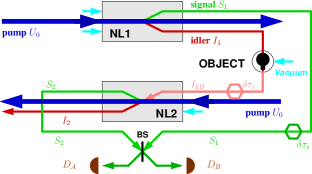
Figure 1: A representation of the QNI scheme (e.g. [27]). The two identical pump fields are in blue, signal fields in green, and idler in red; here the FWM process combines two pump photons to create a signal-idler pair. The resulting signal fields then interfere at the beamsplitter (BS) and detected at $D_{A}$ and $D_{B}$. In an Imperial experiment [28], the nonlinear stages (NL1 and NL2) take place in opposite directions through the same length of fibre.

The nonlinear propagation model in our simulations is a well-established one derived originally for the prediction of squeezing generation in optical fibres [29, 30, 31, 32, 36], has also been used to model multi-field parametric processes [37], and here centres primarily on multi-field nonlinear propagation through a dispersive material. It also includes stages representing setting up the initial conditions, interaction with an object to be imaged, and mixing at a beamsplitter at the interferometer output. In this work we use an established off-diagonal coherent state basis positive-P approach [38, 39, 40], that enables both group velocity and dispersion to be easily implemented in a numerical scheme [29]; crucially, its off-diagonal nature allows a complete representation of the full quantum mechanical density matrix of the system, and of its dynamics.

Our description uses time-dependent quasi-conjugate pump field amplitudes ${\alpha}_{u}\vphantom{{\alpha}_{i}^{\dagger}}(t)$, ${\alpha}_{u}^{\dagger}\vphantom{{\alpha}_{u}^{\dagger}}(t)$, which are only complex-conjugate on average; likewise for signal ${\alpha}_{s}\vphantom{{\alpha}_{i}^{\dagger}}(t)$, ${\alpha}_{s}^{\dagger}\vphantom{{\alpha}_{s}^{\dagger}}(t)$, and idler ${\alpha}_{i}\vphantom{{\alpha}_{i}^{\dagger}}(t)$, ${\alpha}_{i}^{\dagger}\vphantom{{\alpha}_{i}^{\dagger}}(t)$. There is also a set of independent time-dependent noise increments $\{dW_{a}(t)\}$. In simulation, time is discretized and labels a set of finely divided, sub-pulse length modes where each field is held as an array of sequential “time-bins” at $t\in\{t_{j}\}$, each of which contains pairs of complex field amplitudes; these interact and evolve as the fields propagate step-by-step through space. Since these time-bins have a simulation-specific duration, field averages such as $<\!\!{\alpha}_{s}^{\dagger}\vphantom{{\alpha}_{s}^{\dagger}}{\alpha}_{s}\vphantom{{\alpha}_{i}^{\dagger}}\!\!>$ represent intensity (in photons per second), not photon number, and normalizations and parameter scalings reflect this.

This field information is held along with fixed parameters for the nonlinear coupling $\kappa$, losses $\gamma_{m}$, and dispersive properties $D_{m}(\omega)$, where the field subscripts, as above, are $m\in\{u,s,i,r\}$. Since this is a stochastic technique, very many independent copies of the evolution need to be run (for the simulations here, typically in the range $10^{5}$ to $10^{7}$), and the necessary ensemble averages taken.

This propagation model is very close to previous ones (e.g. [29, 32, 37]), but here we have three co-propagating fields and a different nonlinear interaction; namely one for the degenerate FWM process with only resonant wave mixing terms where $2\omega_{u}=\omega_{s}+\omega_{i}$. Since self-phase modulation (SPM) terms are not significant in the low-power regime (see e.g. [28], the interaction Hamiltonian we need here is simply

$$\hat{H}_{\textup{fwm}} =\imath\,{\mathchar 22\relax\mkern-9.0muh}{\vphantom{\chi^{*}}\chi}\hat{a}_{u}^{\dagger}\vphantom{a}{}^{2}\hat{a}_{s}^{\vphantom{\dagger}}\hat{a}_{i}^{\vphantom{\dagger}}-\imath\,{\mathchar 22\relax\mkern-9.0muh}{\vphantom{\chi^{*}}\chi}^{*}\hat{a}_{u}^{\vphantom{\dagger}}\vphantom{a}{}^{2}\hat{a}_{s}^{\dagger}\hat{a}_{i}^{\dagger}.$$ (1)

This interaction term results in propagation equations which are best expressed in the incremental form suited to such stochastic differential equations (SDEs) [38]. In an appropriate co-moving frame, including loss along with nonlinear effects [32], but suppressing the time argument common to all fields ${\alpha}_{m}\vphantom{{\alpha}_{i}^{\dagger}},{\alpha}_{m}^{\dagger}\vphantom{{\alpha}_{m}^{\dagger}}$ and quantum noise increments $dW_{a}$, we have

$$d{\alpha}_{s}\vphantom{{\alpha}_{i}^{\dagger}} =\left[-\gamma_{s}{\alpha}_{s}\vphantom{{\alpha}_{i}^{\dagger}}+{\vphantom{\chi^{*}}\chi}^{*}{\alpha}_{u}\vphantom{{\alpha}_{i}^{\dagger}}{\alpha}_{u}\vphantom{{\alpha}_{i}^{\dagger}}{\alpha}_{i}^{\dagger}\vphantom{{\alpha}_{i}^{\dagger}}\right]dz~{}~{}+\left\{(2{\vphantom{\chi^{*}}\chi})^{{\scalebox{0.6}{1/2}}}{\alpha}_{u}\vphantom{{\alpha}_{i}^{\dagger}}\right\}dW_{1},$$ (2)

$$d{\alpha}_{s}^{\dagger}\vphantom{{\alpha}_{s}^{\dagger}} =\left[-\gamma_{s}{\alpha}_{s}^{\dagger}\vphantom{{\alpha}_{s}^{\dagger}}+{\vphantom{\chi^{*}}\chi}{\alpha}_{u}^{\dagger}\vphantom{{\alpha}_{u}^{\dagger}}{\alpha}_{u}^{\dagger}\vphantom{{\alpha}_{u}^{\dagger}}{\alpha}_{i}\vphantom{{\alpha}_{i}^{\dagger}}\right]dz~{}~{}+\left\{(2{\vphantom{\chi^{*}}\chi}^{*})^{{\scalebox{0.6}{1/2}}}{\alpha}_{u}^{\dagger}\vphantom{{\alpha}_{u}^{\dagger}}\right\}~{}dW_{2},$$ (3)

$$d{\alpha}_{i}\vphantom{{\alpha}_{i}^{\dagger}} =\left[-\gamma_{i}{\alpha}_{i}\vphantom{{\alpha}_{i}^{\dagger}}+{\vphantom{\chi^{*}}\chi}^{*}{\alpha}_{u}\vphantom{{\alpha}_{i}^{\dagger}}{\alpha}_{u}\vphantom{{\alpha}_{i}^{\dagger}}{\alpha}_{s}^{\dagger}\vphantom{{\alpha}_{s}^{\dagger}}\right]dz~{}~{}+\left\{(2{\vphantom{\chi^{*}}\chi})^{{\scalebox{0.6}{1/2}}}{\alpha}_{u}\vphantom{{\alpha}_{i}^{\dagger}}\right\}~{}dW_{1},$$ (4)

$$d{\alpha}_{i}^{\dagger}\vphantom{{\alpha}_{i}^{\dagger}} =\left[-\gamma_{i}{\alpha}_{i}^{\dagger}\vphantom{{\alpha}_{i}^{\dagger}}+{\vphantom{\chi^{*}}\chi}{\alpha}_{u}^{\dagger}\vphantom{{\alpha}_{u}^{\dagger}}{\alpha}_{u}^{\dagger}\vphantom{{\alpha}_{u}^{\dagger}}{\alpha}_{s}\vphantom{{\alpha}_{i}^{\dagger}}\right]dz~{}~{}+\left\{(2{\vphantom{\chi^{*}}\chi}^{*})^{{\scalebox{0.6}{1/2}}}{\alpha}_{u}^{\dagger}\vphantom{{\alpha}_{u}^{\dagger}}\right\}~{}dW_{2},$$ (5)

$$d{\alpha}_{u}\vphantom{{\alpha}_{i}^{\dagger}} =\left[-\gamma_{u}{\alpha}_{u}\vphantom{{\alpha}_{i}^{\dagger}}-2{\vphantom{\chi^{*}}\chi}{\alpha}_{u}^{\dagger}\vphantom{{\alpha}_{u}^{\dagger}}{\alpha}_{s}\vphantom{{\alpha}_{i}^{\dagger}}{\alpha}_{i}\vphantom{{\alpha}_{i}^{\dagger}}\right]dz~{}~{}+\imath\left\{2{\vphantom{\chi^{*}}\chi}^{\vphantom{*}}{\alpha}_{s}\vphantom{{\alpha}_{i}^{\dagger}}{\alpha}_{i}\vphantom{{\alpha}_{i}^{\dagger}}\right\}^{\!\!{\scalebox{0.6}{1/2}}}\!\!\!dW_{3},$$ (6)

$$d{\alpha}_{u}^{\dagger}\vphantom{{\alpha}_{u}^{\dagger}} =\left[-\gamma_{u}{\alpha}_{u}^{\dagger}\vphantom{{\alpha}_{u}^{\dagger}}-2{\vphantom{\chi^{*}}\chi}^{*}\!{\alpha}_{u}\vphantom{{\alpha}_{i}^{\dagger}}{\alpha}_{s}^{\dagger}\vphantom{{\alpha}_{s}^{\dagger}}{\alpha}_{i}^{\dagger}\vphantom{{\alpha}_{i}^{\dagger}}\right]dz+\imath\left\{2{\vphantom{\chi^{*}}\chi}^{*}\!\!{\alpha}_{s}^{\dagger}\vphantom{{\alpha}_{s}^{\dagger}}{\alpha}_{i}^{\dagger}\vphantom{{\alpha}_{i}^{\dagger}}\right\}^{\!\!{\scalebox{0.6}{1/2}}}\!\!\!dW_{4}.\!\!$$ (7)

These equations are used to update each time-bin in the temporal profile of the fields as they propagate (step) forward in space. Deterministic evolution terms are in square brackets $[...]$, and prefactors for stochastic (noisy) terms in braces $\{...\}$. The noises are uncorrelated, with $\delta_{ab}=<dW_{a}(t)dW_{b}(t)>$.

Here we see that there are both coherent interactions between the three fields, and correlated nonlinear quantum noise terms. The noise increment $dW_{1}$ drives both ${\alpha}_{s}\vphantom{{\alpha}_{i}^{\dagger}}$ and ${\alpha}_{i}\vphantom{{\alpha}_{i}^{\dagger}}$, whilst $dW_{2}$ drives ${\alpha}_{s}^{\dagger}\vphantom{{\alpha}_{s}^{\dagger}}$ and ${\alpha}_{i}^{\dagger}\vphantom{{\alpha}_{i}^{\dagger}}$, ensuring the pairs are correlated but not complex conjugate. The comparable classical model (or even a semi-classical model, see e.g. [33, 34, 35]) would have only three equations and no noise terms.

Material dispersion is the other key feature, and we interleave it with the nonlinearity in a split-step scheme (see e.g. Carter et al.[29, 32]), using linear phase shifts in the spectral domain for group velocity, and quadratic shifts for GVD.

Material parameters in the simulations are chosen to be compatible with fiber-based photon pair sources based on spontaneous four-wave mixing [28], which use about $100$cm of Thorlabs PM780-HP fibre (see Table 1). For the simulation, we convert parameters into units based on meters (m), picoseconds (ps), and field excitation amplitudes referenced back to photon numbers per picosecond. A crucial step here is to consider pulsed operation on a picosecond scale, where the group velocity mismatches are significant. This regime is where the time-dependent nature of the entanglement will be most exposed to the disruptive effects of material dispersion.

Since the effect of group velocity mismatches and GVD turns localised entanglements into temporally distributed ones in our simulations we see a fan of signal amplitudes that spreads out behind the pump pulse, whilst a fan of idler amplitudes spreads out before. Thus, crucially, the signal-idler entanglement is not only distributed over a range of times, it is also between different times; i.e. it is a multi-time correlation. For best imaging visibility, this requires careful synchronisation at NL2, where the first-generated part of the idler in NL2 should be coincident with the pump pulse as it enters.

Field	Wavelength	Frequency	$\Delta v_{g}$	Dispersion $d_{2}$
Pump	768 nm	390.5 THz	0 ps/m	0.589 ps2/km
Signal	700 nm	428.0 THz	-100 ps/m	0.489 ps2/km
Idler	850 nm	353.0 THz	+83 ps/m	0.721 ps2/km

Table 1: Material parameters used in the simulations, based on the experimental setup of [28]. Since the fibre is weakly guiding, these are based on those for bulk silica. The nonlinearity in SI units is $n_{2}=3\times 10^{-20}$m${}^{2}/$W, and the loss is $\gamma=0.004/$m. In simulation units, the PM780-HP’s stated transverse field mode area of about 25$\mu$m² and the pump photon energy of $25\times 10^{-20}$J, means that the rescaled nonlinearity is $n^{\prime\prime}_{2}=0.3\times 10^{-15}$ per photon-picosecond. In a time-bin $T$ ps long, the pump photon has a power $\sim(0.25/T)$ $\mu$W, so that a power of $100$W corresponds to a flux of $4\times 10^{8}$ photons/ps. Estimates for signal and idler fields are similar. Note that the pump powers used in the simulations are increased to enable good simulation statistics (see Supplementary information).

Objects placed in the idler beam leaving the NL1 stage disrupt the entanglement with the signal beam, and that disruption changes the numbers of detected photons, enabling the object’s presence or properties to be inferred. However, in non-imaging contexts, we can view them as representatives of further disruptive unwanted real-world effects: loss, phase shifts through optical elements, or extraneous couplings. Here we consider passive objects that impart (a) a phase modulation $\Delta\phi$ of the idler field, or have (b) a reflectivity $r$ that reduces the idler amplitudes as they pass (as in [27]); so $r=1$ removes all entanglement. We also consider (c) imaging of dynamic objects, a key feature since an object’s time dependence will affect visibility, just as timing, group velocity, and GVD do.

Our linearly coupled dynamic objects with amplitudes $\beta(t),\beta^{\dagger}(t)$ respond to the incident pulse profile $\alpha_{m}(t),\alpha_{m}^{\dagger}(t)$ at the position $z$ specific to the object; and a field-object interaction strength $\eta$. At the object we set the initial conditions at $t_{o}$ so that $\beta(t_{o})=\beta_{o}$ and $\beta^{\dagger}(t_{o})=\beta^{*}_{o}$, and then time integrate $\beta(t),\beta^{\dagger}(t)$ using

$$d\beta(t) =\left[-\gamma_{o}\beta(t)+\eta^{*}\alpha_{m}(t)\right]~{}dt,$$ (8)

$$d\beta^{\dagger}(t) =\left[-\gamma_{o}\beta^{\dagger}(t)+\eta^{~{}}\alpha_{m}^{\dagger}(t)\right]~{}dt.$$ (9)

Now that the incident field $\alpha_{m},\alpha_{m}^{\dagger}$ has excited the dynamic object, this excitation acts back on the field and modifies it. We therefore then update $\alpha(t),\alpha^{\dagger}(t)$ according to the same linear interaction but here integrated forward in space, using

$$d\alpha_{m}(t) =-\tfrac{1}{2}\eta^{~{}}\beta(t)~{}dz;\quad d\alpha_{m}^{\dagger}(t)=-\tfrac{1}{2}\eta^{*}\beta^{\dagger}(t)~{}dz,$$ (10)

and keeping the SDE notation for consistency. Note that this could be extended to allow for nonlinear couplings or dynamics with the object, or to even use (e.g.) a two-level-atom or Raman models (see e.g. a classical counterpart [41]).

Detection and Visibility: The photon number rate measured at the detectors is taken to be the ensemble-averaged photon number of the relevant field at that point. An improved detector model could be implemented using similar approach to time-dependent objects. An important quantity is the visibility of the entanglement, which is the difference of the detector counts (“signal”) divided by the sum of the detector counts (“background”); i.e. $|n_{A}-n_{B}|/(n_{A}+n_{B})$. To suppress sampling artifacts in the pulse wings we add to the background an offset of $0.05$% of its maximum.

We test the basics of the simulations with a simple CW-equivalent parameter set with no group velocity or GVD effects, and look at how the visibility varies with object phase-shifts and object reflectivities. Here, correlations between the first signal’s time-bins and the second signal’s ones will always be synchronised, maximizing the visibility. For sufficiently low signal-idler generation efficiencies, we should see equal photon number intensities in the signal’s field-modes, but distinct photon number intensities after the beamsplitter, i.e. at the two detectors; this is clearly shown on fig. 2.

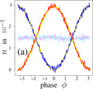
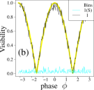
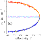
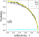
Figure 2: Entanglement visibility measurement versus a specified phase shift (top) and reflectivity (bottom) caused by an imaged object: (a,c) Photon counts at detectors $D_{A}$, $D_{B}$ (in red and blue), compared to photon numbers in the pre-beamsplitter signal fields $S_{1}$, $S_{2}$ (dashed, in cyan and magenta). (b,d) visibility based on detector measurements (black) compared against one calculated from signal fields (cyan). On (c,d), the $r=1$ end result gives the case of a blocking object, i.e. no entanglement. Statistical noise can be reduced by increasing the ensemble sizes from 256k, but are retained as-is to emphasise the necessity of the ensemble averaging. The results match the theoretical fits shown in the background as thick yellow lines.

Time averaging is a crucial part of any detection model used here, since real detectors are very slow (typically $\gg 100$ps) when compared to the temporal resolution of our simulations ($\sim$ps). Although more sophisticated models can easily be imagined, here we simply sum the time-binned amplitudes of each field over some chosen $m$-bin detector response time, before ensemble averaging to get the detected photons:

$$\bar{n}_{D} =<\bar{\alpha}^{\dagger}\bar{\alpha}^{\vphantom{\dagger}}>,\quad\textrm{with}~{}~{}\bar{\alpha}^{(\dagger)}={(\tfrac{1}{m})}^{\!{\scalebox{0.6}{1/2}}}{\sum}_{i=1}^{m}\alpha^{(\dagger)}(t_{i}).$$ (11)

Crucially, this averaging process in the detector helps expose correlations between time-bins that have become offset due to dispersion mismatches. Note that this summation is essentially the same as the process for combining multiple short time bins into a longer one; just as we need to do in numerical convergence checks. On fig. 3, the entanglement is always fully present, but has its visibility reduced by $v_{g}$ or GVF mismatch. However visibility can be recovered using longer averaging intervals; at least up to a ($v_{g}$) cut-off when the time difference exceeds the averaging windows.

Figure 3: Detectable entanglement is obscured by material dispersion, even though the entanglement itself remains: the no-object case, as group velocity ($v_{g}$) and GVD mismatches increase, for 100cm propagation with standard parameters, and comparing detection time-averaging intervals. Here the mismatch is applied to the signal field $S_{1}$, so that a $v_{g}$ mismatch causes a timing offset $\delta\tau_{s}$ at the beamsplitter. Circles ($\circ$) are “fast detector” un-averaged results, other symbols show the number of adjacent $0.5$ps time-bins averaged. For $v_{g}$ mismatches (a), the regular residual bumps in $\circ$ are a discretization artifact, and can be further suppressed by increasing the time resolution. The complicated effect of GVD mismatches (b) leads to smooth variations as different contributions de-phase or rephase.

Pulsed simulations: Here we standardise on an input 40ps pump pulse and a 512ps window divided into $2$ps bins. Simulation pulse intensities were chosen as low as practicable, given the constraints of computation time and the requirement for good simulation statistics. Further, the pump-idler pulses were ideally synchronised as they entered the NL2 stage. However, the signal fields are also mis-timed at the output beamsplitter by $\delta\tau_{s}={20}$ps (i.e. 10 time bins). This not only mimics imperfect experimental setup, it is also useful in providing an example where the detector averaging has more to recover. We also use a technique, described in the Supplementary Material, to reduce the effect of sampling error – something which would otherwise make positive-P simulations either problematic or computationally prohibitive.

Results for no object and standard material parameters, but also considering artificially reduced group velocity offsets, are shown on fig. 4(a-f), where they are compared with full parameter results. The displacement to negative $t$ of the visibility peak is a result of the group velocity walk-off of the signal field. We see that the detected photon rates $n$ decrease at larger group velocity mismatches – this is due to the increased spreading of the generated fields, and hence less effective nonlinear generation. Despite the decrease in detected $n$, we see that the reduction in detector-averaged entanglement visibility is relatively minor; whilst in stark contrast, the drop in un-averaged visibility is significant. Thus we see that sufficiently long averaging interval allows us to recover most of the maximum possible visibility, albeit not all; and as we would expect the averaging also helps reduce the significant statistical variation visible on the un-averaged data. Thus fig. 4 shows that group velocity mismatches are not as problematic as they might at first appear, since the generated entanglements, however scrambled they might be by the gradual nonlinear generation and significantly dispersive propagation, can be recovered to a significant extent by time-averaging at the detector.

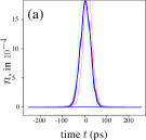
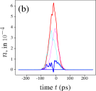
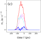
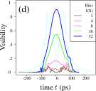
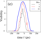
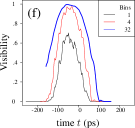
Figure 4: Pulsed simulations with no object ($r=0$) and artificially scaled ((a,d) 10%, (b,e) 50%) and true (c,f) group velocity offsets.  (a,b,c): detected photon numbers per 2ps, $n_{A},n_{B}$ (red and blue); dotted lines are $n_{s1},n_{s2}$ for the pre-beamsplitter signal fields; note the change in vertical axis scale.  (d,e,f): detected entanglement visibilities for different time averaging, at 2ps per bin; note that statistical fluctuations artificially increase the computed visibility. The 1(S) curve on (d) is a (false) visibility based on the pre-beamsplitter signal pulses, and has a value only because of their arrival-time mismatch.

In fig. 4 the simulations ensured the idler pulse arrived at the NL2 stage in correct synchronization with the pump pulse. We can see the effect of mis-timing the idler pulse at this point on fig. 5(a), where at least for these parameters – notably 40ps pulse widths – the fall off in averaged visibility is gradual. This is due to a combination of the pump pulse length ($40$ps), the averaging time ($64$ps), and the group velocity spreading ($\sim 80$ps). On fig. 5(b,c), and in broad agreement with trends in fig. 2, we see a fall-off of the time-dependent entanglement visibility with object phase depth and object reflectivity.

Dynamic objects further emphasise the potential role of time-dependence. Fig. 5(d) shows recovered entanglement visibility values for a range of interaction strengths $\eta^{\prime}$. At low $\eta^{\prime}$, idler field excitations are coupled into the object but not out again, leading to reduced visibility. However, as the $\eta^{\prime}$ increases even further, those excitations can also start being coupled back out, leading to a partial recovery. This non-trivial behaviour suggests the possibility of interesting trade-offs when considering the imaging of dynamic objects.

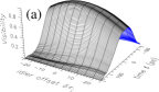
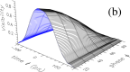
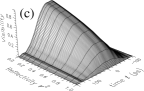
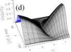
Figure 5: Time-dependent entanglement visibilities for pulsed simulations with 32 bin (64ps) averaging and a $40$ps mistiming at the output beamsplitter. In (a) we see how the visibility profile changes if the idler synchonisation $\delta\tau_{i}$ differs from the ideal value. Other frames show results for varying object properties, i.e. (b) phase, (c) reflectivity, and (d) interaction with a dynamic object as per (8) – (10).

In conclusion, we have shown how the time-averaging process inherent in slow detector response times enables recovery of the entanglement necessary quantum nonlinear interferometry, even when confounding effects such as group velocity differences, dispersion, mis-timing of pulse arrivals, or objects interposed in the idler beam are allowed for. Indeed, group velocity mismatches would normally be expected to play a critical role, seeing as they can rapidly de-synchronise mutually entangled time-slices of the light field. This can be seen in our simulation results (e.g. in figs. 3(a) and 4(f)) which show a significant improvement when changing from un-averaged to averaged visibilities. In contrast to visibilities, which are a ratio, nonlinear generation efficiencies suffer penalties from the effect of material dispersion regardless of averaging. Finally, our linearly coupled dynamic object model acts as a starting point for more sophisticated interactions; a feature likely to be important in systems relying on short pulses, resonant behaviour, and time-domain entanglement.

Acknowledgements: Support from the UK National Quantum Hub for Imaging (QUANTIC, EP/T00097X/1).

Supplementary Information:
 
The surprising persistence of time-dependent quantum entanglement

Paul Kinsler, Martin W. McCall, Rupert F. Oulton, and Alex S. Clark
Department of Physics, Imperial College London, United Kingdom

.1 Representation of entanglement

In the model used here, entanglement is represented as classical statistical correlations between complex field amplitudes which are capable of reproducing the off-diagonal elements of the density matrix – i.e. they can represent all the necessary quantum properties [38]. This is possible because each field is represented by two independent amplitudes $\alpha_{m}$ and $\alpha_{m}^{\dagger}$; and although they are complex conjugate on average, i.e. $<\alpha_{m}>=<\alpha_{m}^{\dagger}>^{*}$, in any given trajectory making up part of the large ensemble, they need not be.

By looking at the SDE’s for the nonlinearity (2) – (7), we can see that the non-daggered and the daggered amplitudes are driven by different noises. Thus both the mean photon numbers $<{\alpha}_{s}^{\dagger}\vphantom{{\alpha}_{s}^{\dagger}}{\alpha}_{s}\vphantom{{\alpha}_{i}^{\dagger}}>$ and $<{\alpha}_{i}^{\dagger}\vphantom{{\alpha}_{i}^{\dagger}}{\alpha}_{i}\vphantom{{\alpha}_{i}^{\dagger}}>$ could even remain nearly zero even whilst a significant quantum statistical correlation (i.e. entanglement) is being created between the signal and idler fields; i.e. between ${\alpha}_{s}\vphantom{{\alpha}_{i}^{\dagger}}$ and ${\alpha}_{s}^{\dagger}\vphantom{{\alpha}_{s}^{\dagger}}$, and between ${\alpha}_{s}^{\dagger}\vphantom{{\alpha}_{s}^{\dagger}}$ and ${\alpha}_{i}^{\dagger}\vphantom{{\alpha}_{i}^{\dagger}}$.

.2 Simulation statistics: reducing sampling error

It has long been known that that getting good simulation statistics with the fully quantum mechanical positive-P representation can be challenging [32], so that it is very common to resort to the much simpler, but approximate, truncated Wigner representation [40] in simulations. In cantrast to the positive-P, the truncated Wigner representation is essentially a semi-classical hidden variable model that represents the quantum uncertainty as simple statistical fluctuations in the field amplitudes [33, 34]. This halves the number of equations required by the simulation (needing only a single complex $\alpha$ rather than the double $\alpha$ and $\alpha^{\dagger}$), reducing the state space, and resulting in an effective and sufficiently accurate method when e.g. studying quadrature squeezing [42], and its generation using optical pulses in nonlinear materials [29, 30, 32, 36].

However, in this work, here we want to ensure an accurate representation of the quantum effects, and so we stay with the full positive-P model (cf the case of quantum tunnelling [33, 34] and nonlinearity and the quantum vacuum [35]). Since the subtler effects of quantum entanglement is addressed here, rather than the simpler quadrature moments, a truncated Wigner representation would not suffice, since it imposes an unavoidable linkage between correlations and photon number. This leaves us requiring the use of a full positive-P description and concommitant extremely long run times. This is especially problematic since we may need to resolve very low average photon numbers inside an extremely noisy background.

We address this using a hybrid strategy which allows us to use just one very high ensemble number $M_{B}$ simulation to get a good estimate of the background for some particular case, and then adjusting this using two more simulations with lower ensemble numbers $M_{R}$ but perfectly matched random noise generation. We call the $M_{B}$ simulation the “background”, and the other two the “reference” and “target” simulations. The reference simulation has identical parameters to the background simulations, and the target simulation has the parameters coresponding to the particular result we are interested in. The difference between the reference and target simulations only depends on the differences between the system parameters, with only “second-order” noise effects – resulting from how the noise influences propagation differently, and not from different random number sequences.

When trying to evaluate a photon number $n$ for some chosen target parameters, we proceed as follows, using the usual notation where a statistical average is denoted $<n>$, but additionally adding a subscript to denote the ensemble size, with $\infty$ to denote the idea infinite-ensemble case. Each trajectory in the background or reference ensembles returns a value $n^{\prime}_{j}$, and each in the target ensemble returns $n_{j}$.

Thus for $n^{\prime}$ we can have either a low sampling error, or a larger sampling error, as follows

$$\left<n^{\prime}\right>_{\infty} \simeq\left<n^{\prime}\right>_{M_{B}}=\frac{1}{M_{B}}\sum_{j=1}^{M_{B}}n^{\prime}_{j}$$ (12)

$$\approx\left<n^{\prime}\right>_{M_{R}}=\frac{1}{M_{R}}\sum_{j=1}^{M_{R}}n^{\prime}_{j},$$ (13)

with the sampling error reducing for each as $M_{B}$ and $M_{R}$ are increased; thus for large enough $M$ values we have

$$\left<n^{\prime}\right>_{M_{B}} \approx\left<n^{\prime}\right>_{M_{R}}$$ (14)

$$\textrm{i.e.}\qquad\left<n^{\prime}\right>_{M_{B}}-\left<n^{\prime}\right>_{M_{R}} \approx 0,$$ (15)

but noting that the noise-sampling error in this approximate equality (15) is dominated by the larger variation in the smaller reference ensemble.

Similarly, for $n$ we we have

$$\left<n\right>_{\infty} \approx\left<n\right>_{M_{R}}=\frac{1}{M_{R}}\sum_{j=1}^{M_{R}}n_{j}.$$ (16)

Since (15) should average to zero, we can now write

$$\left<n\right>_{\infty} =\left<n\right>_{\infty}-\left<n^{\prime}\right>_{\infty}+\left<n^{\prime}\right>_{\infty}$$ (17)

$$\approx\left<n\right>_{M_{R}}-\left<n^{\prime}\right>_{M_{R}}-\left<n^{\prime}\right>_{M_{B}},$$ (18)

which, given its dependence on both $\left<n\right>_{M_{R}}$ and $\left<n^{\prime}\right>_{M_{R}}$, would at first appear to suffer a larger sampling error based on the smaller $M_{R}$, not a small sampling error based on the large $M_{B}$.

However, the key point is that since we have exactly matched the simulation noise values between the reference simulations of $n^{\prime}_{j}$ and target simulations of $n_{j}$ then their difference is due to differences of the trajectory dynamics between the two simulations, and is only weakly dependent on the specific noise values. Since this cancels out the bulk of the sampling error due to the noise in these smaller-ensemble simulations, we can now write

$$\left<n\right>_{\infty} \simeq\left<n\right>_{M_{R}}-\left<n^{\prime}\right>_{M_{R}}-\left<n^{\prime}\right>_{M_{B}},$$ (19)

where now it is the sampling error from the background ensemble that dominates.

Thus for any parameter set, we only need to do one large ensemble $M_{B}$ background simulation, one smaller ensemble $M_{R}$ reference simulation otherwise identical to the background one, and then then many small $M_{R}$ target simulations which do have a parameter variation compared to the background simulation. Background parameters were of systems with perfectly transparent objects, and our target simulations varied only the object properties. This meant that all the results shown on fig. 5 could be generated from the same background simulation, a large and – in our case – very necessary reduction in total simulation time.

Here we typically did background simulations with $M_{B}$ sizes from $\sim 10^{6}$ (fig. 4(a,d)) to $\sim 16\times 10^{6}$ (figs. 4(c,f) and 5), and reference and target simulations with $M_{B}=128\times 10^{3}$. In the most extreme case, this gave us a factor of 125 improvement in effective simulation speed, as well as the crucial decrease in statistical error. Whilst it may be possible to vary other parameters, or perhaps even several parameters at once, this will induce a greater divergence between propagation in the reference and target systems, and so affect the extent of any improvement.

.3 Nonlinearity

As described in the main text, the key feature of the degenerate-pump spontaneous FWM interaction used in our simulations is that it produces pairs of entangled signal and idler fields (photons). It shares this feature with the more commonly used second order parametric nonlinearity [40] (usually denoted $\chi^{(2)}$), which generates the same kind of entangled pairs but from single pump photons, not pairs.

Although this difference is not trivial, the SDE equations for a $\chi^{(2)}$ nonlinearity are similar in form, although with no quantum noise term applied to the pump field. To test what differences might appear between the two models, some simulations were also done with this $\chi^{(2)}$ model and system parameters rescaled to match the nonlinear effects; the results were remarkably similar in character, indicating that our conclusions are not specific to the FWM model we present here.

Note that the nonlinear response is treated here as if it were instantaneous. This is a reasonable approximation since typical nonlinear response times in dielectrics are of the order of femtoseconds or less [43].

.4 Evolution: from density matrix to SDEs

Since to our knowledge the positive-P Fokker-Planck equation for the degenerate-pump FWM interaction Hamiltonian are not currently in the literature, so we now sumarize the derivation. This interaction Hamiltonian (1) gives a contribution to the density matrix evolution

$$\dot{\rho}_{\textup{int}} =\frac{\imath}{\,{\mathchar 22\relax\mkern-9.0muh}}\left[\hat{H}_{\textup{int}},\rho\right].$$ (20)

The expansion of the density matrix in terms of coherent states, albeit for just a single mode, is

$$\rho =\int\frac{\left|\alpha\right>\left<\alpha^{\dagger}\right|}{\left<\alpha|\alpha^{\dagger}\right>}P(\alpha,\alpha^{\dagger};t)~{}d^{2}\alpha~{}d^{2}\alpha^{\dagger}.$$ (21)

Using the standard positive-P operator correspondences, we can convert the density matrix dynamics into a dynamics for the corresponding positive-P distribution function [38, 39, 40]. which is a function of many complex coherent state amplitudes. The resulting Fokker-Planck equation for this $P(...;t)$ is

$$\partial_{t}P(...;t) =\mathscr{L}_{\textup{int}}P(...;t).$$ (22)

The derivative operators defining this part of the dynamics for the positive-P distribution $P$ is as follows. The first two lines result from the first commutator term $\hat{H}_{\textup{int}}\rho$, and the last two lines from $-\rho\hat{H}_{\textup{int}}$, are

$$\mathscr{L}_{\textup{int}} =-{\vphantom{\chi^{*}}\chi}\left({\alpha}_{u}^{\dagger}\vphantom{{\alpha}_{u}^{\dagger}}+\frac{\partial}{\partial{{\alpha}_{u}\vphantom{{\alpha}_{i}^{\dagger}}}}\right)^{2}{\alpha}_{s}\vphantom{{\alpha}_{i}^{\dagger}}{\alpha}_{i}\vphantom{{\alpha}_{i}^{\dagger}}$$

$$\quad+{\vphantom{\chi^{*}}\chi}^{*}{\alpha}_{u}\vphantom{{\alpha}_{i}^{\dagger}}{\alpha}_{u}\vphantom{{\alpha}_{i}^{\dagger}}\left({\alpha}_{s}^{\dagger}\vphantom{{\alpha}_{s}^{\dagger}}+\frac{\partial}{\partial{{\alpha}_{s}\vphantom{{\alpha}_{i}^{\dagger}}}}\right)\left({\alpha}_{i}^{\dagger}\vphantom{{\alpha}_{i}^{\dagger}}+\frac{\partial}{\partial{{\alpha}_{i}\vphantom{{\alpha}_{i}^{\dagger}}}}\right)$$

$$\quad\quad+{\vphantom{\chi^{*}}\chi}{\alpha}_{u}^{\dagger}\vphantom{{\alpha}_{u}^{\dagger}}{\alpha}_{u}^{\dagger}\vphantom{{\alpha}_{u}^{\dagger}}\left({\alpha}_{s}\vphantom{{\alpha}_{i}^{\dagger}}+\frac{\partial}{\partial{{\alpha}_{s}^{\dagger}\vphantom{{\alpha}_{s}^{\dagger}}}}\right)\left({\alpha}_{i}\vphantom{{\alpha}_{i}^{\dagger}}+\frac{\partial}{\partial{{\alpha}_{i}^{\dagger}\vphantom{{\alpha}_{i}^{\dagger}}}}\right)$$

$$\quad\quad\quad-{\vphantom{\chi^{*}}\chi}^{*}\left({\alpha}_{u}\vphantom{{\alpha}_{i}^{\dagger}}+\frac{\partial}{\partial{{\alpha}_{u}^{\dagger}\vphantom{{\alpha}_{u}^{\dagger}}}}\right)^{2}{\alpha}_{s}^{\dagger}\vphantom{{\alpha}_{s}^{\dagger}}{\alpha}_{i}^{\dagger}\vphantom{{\alpha}_{i}^{\dagger}}.$$ (23)

Expanded we have,

$$-{\vphantom{\chi^{*}}\chi}\left\{{\alpha}_{u}^{\dagger}\vphantom{{\alpha}_{u}^{\dagger}}{\alpha}_{u}^{\dagger}\vphantom{{\alpha}_{u}^{\dagger}}+{\alpha}_{u}^{\dagger}\vphantom{{\alpha}_{u}^{\dagger}}\frac{\partial}{\partial{{\alpha}_{u}\vphantom{{\alpha}_{i}^{\dagger}}}}+\frac{\partial}{\partial{{\alpha}_{u}\vphantom{{\alpha}_{i}^{\dagger}}}}{\alpha}_{u}^{\dagger}\vphantom{{\alpha}_{u}^{\dagger}}+\frac{\partial}{\partial{{\alpha}_{u}\vphantom{{\alpha}_{i}^{\dagger}}}}\frac{\partial}{\partial{{\alpha}_{u}\vphantom{{\alpha}_{i}^{\dagger}}}}\right\}{\alpha}_{s}\vphantom{{\alpha}_{i}^{\dagger}}{\alpha}_{i}\vphantom{{\alpha}_{i}^{\dagger}}$$

$$\quad+{\vphantom{\chi^{*}}\chi}^{*}{\alpha}_{u}\vphantom{{\alpha}_{i}^{\dagger}}{\alpha}_{u}\vphantom{{\alpha}_{i}^{\dagger}}\left\{{\alpha}_{s}^{\dagger}\vphantom{{\alpha}_{s}^{\dagger}}{\alpha}_{i}^{\dagger}\vphantom{{\alpha}_{i}^{\dagger}}+{\alpha}_{s}^{\dagger}\vphantom{{\alpha}_{s}^{\dagger}}\frac{\partial}{\partial{{\alpha}_{i}\vphantom{{\alpha}_{i}^{\dagger}}}}+\frac{\partial}{\partial{{\alpha}_{s}\vphantom{{\alpha}_{i}^{\dagger}}}}{\alpha}_{i}^{\dagger}\vphantom{{\alpha}_{i}^{\dagger}}+\frac{\partial}{\partial{{\alpha}_{s}\vphantom{{\alpha}_{i}^{\dagger}}}}\frac{\partial}{\partial{{\alpha}_{i}\vphantom{{\alpha}_{i}^{\dagger}}}}\right\}$$

$$\quad\quad+{\vphantom{\chi^{*}}\chi}{\alpha}_{u}^{\dagger}\vphantom{{\alpha}_{u}^{\dagger}}{\alpha}_{u}^{\dagger}\vphantom{{\alpha}_{u}^{\dagger}}\left\{{\alpha}_{s}\vphantom{{\alpha}_{i}^{\dagger}}{\alpha}_{i}\vphantom{{\alpha}_{i}^{\dagger}}+{\alpha}_{s}\vphantom{{\alpha}_{i}^{\dagger}}\frac{\partial}{\partial{{\alpha}_{i}^{\dagger}\vphantom{{\alpha}_{i}^{\dagger}}}}+\frac{\partial}{\partial{{\alpha}_{s}^{\dagger}\vphantom{{\alpha}_{s}^{\dagger}}}}{\alpha}_{i}\vphantom{{\alpha}_{i}^{\dagger}}+\frac{\partial}{\partial{{\alpha}_{s}^{\dagger}\vphantom{{\alpha}_{s}^{\dagger}}}}\frac{\partial}{\partial{{\alpha}_{i}^{\dagger}\vphantom{{\alpha}_{i}^{\dagger}}}}\right\}$$

$$\quad\quad\quad-{\vphantom{\chi^{*}}\chi}^{*}\left\{{\alpha}_{u}\vphantom{{\alpha}_{i}^{\dagger}}{\alpha}_{u}\vphantom{{\alpha}_{i}^{\dagger}}+\frac{\partial}{\partial{{\alpha}_{u}^{\dagger}\vphantom{{\alpha}_{u}^{\dagger}}}}{\alpha}_{u}\vphantom{{\alpha}_{i}^{\dagger}}+{\alpha}_{u}\vphantom{{\alpha}_{i}^{\dagger}}\frac{\partial}{\partial{{\alpha}_{u}^{\dagger}\vphantom{{\alpha}_{u}^{\dagger}}}}+\frac{\partial}{\partial{{\alpha}_{u}^{\dagger}\vphantom{{\alpha}_{u}^{\dagger}}}}\frac{\partial}{\partial{{\alpha}_{u}^{\dagger}\vphantom{{\alpha}_{u}^{\dagger}}}}\right\}{\alpha}_{s}^{\dagger}\vphantom{{\alpha}_{s}^{\dagger}}{\alpha}_{i}^{\dagger}\vphantom{{\alpha}_{i}^{\dagger}}.$$ (24)

Now all the terms without derivatives cancel, so that

$$-{\vphantom{\chi^{*}}\chi}\left\{{\alpha}_{u}^{\dagger}\vphantom{{\alpha}_{u}^{\dagger}}\frac{\partial}{\partial{{\alpha}_{u}\vphantom{{\alpha}_{i}^{\dagger}}}}+\frac{\partial}{\partial{{\alpha}_{u}\vphantom{{\alpha}_{i}^{\dagger}}}}{\alpha}_{u}^{\dagger}\vphantom{{\alpha}_{u}^{\dagger}}+\frac{\partial}{\partial{{\alpha}_{u}\vphantom{{\alpha}_{i}^{\dagger}}}}\frac{\partial}{\partial{{\alpha}_{u}\vphantom{{\alpha}_{i}^{\dagger}}}}\right\}{\alpha}_{s}\vphantom{{\alpha}_{i}^{\dagger}}{\alpha}_{i}\vphantom{{\alpha}_{i}^{\dagger}}$$

$$\quad+{\vphantom{\chi^{*}}\chi}^{*}{\alpha}_{u}\vphantom{{\alpha}_{i}^{\dagger}}{\alpha}_{u}\vphantom{{\alpha}_{i}^{\dagger}}\left\{{\alpha}_{s}^{\dagger}\vphantom{{\alpha}_{s}^{\dagger}}\frac{\partial}{\partial{{\alpha}_{i}\vphantom{{\alpha}_{i}^{\dagger}}}}+\frac{\partial}{\partial{{\alpha}_{s}\vphantom{{\alpha}_{i}^{\dagger}}}}{\alpha}_{i}^{\dagger}\vphantom{{\alpha}_{i}^{\dagger}}+\frac{\partial}{\partial{{\alpha}_{s}\vphantom{{\alpha}_{i}^{\dagger}}}}\frac{\partial}{\partial{{\alpha}_{i}\vphantom{{\alpha}_{i}^{\dagger}}}}\right\}$$

$$\quad\quad+{\vphantom{\chi^{*}}\chi}{\alpha}_{u}^{\dagger}\vphantom{{\alpha}_{u}^{\dagger}}{\alpha}_{u}^{\dagger}\vphantom{{\alpha}_{u}^{\dagger}}\left\{{\alpha}_{s}\vphantom{{\alpha}_{i}^{\dagger}}\frac{\partial}{\partial{{\alpha}_{i}^{\dagger}\vphantom{{\alpha}_{i}^{\dagger}}}}+\frac{\partial}{\partial{{\alpha}_{s}^{\dagger}\vphantom{{\alpha}_{s}^{\dagger}}}}{\alpha}_{i}\vphantom{{\alpha}_{i}^{\dagger}}+\frac{\partial}{\partial{{\alpha}_{s}^{\dagger}\vphantom{{\alpha}_{s}^{\dagger}}}}\frac{\partial}{\partial{{\alpha}_{i}^{\dagger}\vphantom{{\alpha}_{i}^{\dagger}}}}\right\}$$

$$\quad\quad\quad-{\vphantom{\chi^{*}}\chi}^{*}\left\{\frac{\partial}{\partial{{\alpha}_{u}^{\dagger}\vphantom{{\alpha}_{u}^{\dagger}}}}{\alpha}_{u}\vphantom{{\alpha}_{i}^{\dagger}}+{\alpha}_{u}\vphantom{{\alpha}_{i}^{\dagger}}\frac{\partial}{\partial{{\alpha}_{u}^{\dagger}\vphantom{{\alpha}_{u}^{\dagger}}}}+\frac{\partial}{\partial{{\alpha}_{u}^{\dagger}\vphantom{{\alpha}_{u}^{\dagger}}}}\frac{\partial}{\partial{{\alpha}_{u}^{\dagger}\vphantom{{\alpha}_{u}^{\dagger}}}}\right\}{\alpha}_{s}^{\dagger}\vphantom{{\alpha}_{s}^{\dagger}}{\alpha}_{i}^{\dagger}\vphantom{{\alpha}_{i}^{\dagger}}.$$ (25)

Now we organise the terms. Collecting the first derivative terms, which are deterministic “drift” terms, results in

$$-\frac{\partial}{\partial{{\alpha}_{u}\vphantom{{\alpha}_{i}^{\dagger}}}}\left[2{\vphantom{\chi^{*}}\chi}{\alpha}_{u}^{\dagger}\vphantom{{\alpha}_{u}^{\dagger}}{\alpha}_{s}\vphantom{{\alpha}_{i}^{\dagger}}{\alpha}_{i}\vphantom{{\alpha}_{i}^{\dagger}}\right]-\frac{\partial}{\partial{{\alpha}_{u}^{\dagger}\vphantom{{\alpha}_{u}^{\dagger}}}}\left[2{\vphantom{\chi^{*}}\chi}^{*}{\alpha}_{u}\vphantom{{\alpha}_{i}^{\dagger}}{\alpha}_{s}^{\dagger}\vphantom{{\alpha}_{s}^{\dagger}}{\alpha}_{i}^{\dagger}\vphantom{{\alpha}_{i}^{\dagger}}\right]$$

$$\quad+\frac{\partial}{\partial{{\alpha}_{s}\vphantom{{\alpha}_{i}^{\dagger}}}}\left[{\vphantom{\chi^{*}}\chi}^{*}{\alpha}_{u}\vphantom{{\alpha}_{i}^{\dagger}}{\alpha}_{u}\vphantom{{\alpha}_{i}^{\dagger}}{\alpha}_{i}^{\dagger}\vphantom{{\alpha}_{i}^{\dagger}}\right]+\frac{\partial}{\partial{{\alpha}_{s}^{\dagger}\vphantom{{\alpha}_{s}^{\dagger}}}}\left[{\vphantom{\chi^{*}}\chi}{\alpha}_{u}^{\dagger}\vphantom{{\alpha}_{u}^{\dagger}}{\alpha}_{u}^{\dagger}\vphantom{{\alpha}_{u}^{\dagger}}{\alpha}_{i}\vphantom{{\alpha}_{i}^{\dagger}}\right]$$

$$\quad\quad+\frac{\partial}{\partial{{\alpha}_{i}\vphantom{{\alpha}_{i}^{\dagger}}}}\left[{\vphantom{\chi^{*}}\chi}^{*}{\alpha}_{u}\vphantom{{\alpha}_{i}^{\dagger}}{\alpha}_{u}\vphantom{{\alpha}_{i}^{\dagger}}{\alpha}_{s}^{\dagger}\vphantom{{\alpha}_{s}^{\dagger}}\right]+\frac{\partial}{\partial{{\alpha}_{i}^{\dagger}\vphantom{{\alpha}_{i}^{\dagger}}}}\left[{\vphantom{\chi^{*}}\chi}{\alpha}_{u}^{\dagger}\vphantom{{\alpha}_{u}^{\dagger}}{\alpha}_{u}^{\dagger}\vphantom{{\alpha}_{u}^{\dagger}}{\alpha}_{s}\vphantom{{\alpha}_{i}^{\dagger}}\right].$$ (26)

These can be immediately converted into SDE drift terms where the leading derivative supplies the “which field” information and the argument (in square brackets “[…]”) supplies the change in that field.

Collecting the second derivative terms, which are noise-like diffusion terms, results in

$$-\frac{1}{2}\frac{\partial}{\partial{{\alpha}_{u}\vphantom{{\alpha}_{i}^{\dagger}}}}\frac{\partial}{\partial{{\alpha}_{u}\vphantom{{\alpha}_{i}^{\dagger}}}}\left\{2{\vphantom{\chi^{*}}\chi}{\alpha}_{s}\vphantom{{\alpha}_{i}^{\dagger}}{\alpha}_{i}\vphantom{{\alpha}_{i}^{\dagger}}\right\}-\frac{1}{2}\frac{\partial}{\partial{{\alpha}_{u}^{\dagger}\vphantom{{\alpha}_{u}^{\dagger}}}}\frac{\partial}{\partial{{\alpha}_{u}^{\dagger}\vphantom{{\alpha}_{u}^{\dagger}}}}\left\{2{\vphantom{\chi^{*}}\chi}^{*}{\alpha}_{s}^{\dagger}\vphantom{{\alpha}_{s}^{\dagger}}{\alpha}_{i}^{\dagger}\vphantom{{\alpha}_{i}^{\dagger}}\right\}$$

$$\quad+\frac{1}{2}\frac{\partial}{\partial{{\alpha}_{s}\vphantom{{\alpha}_{i}^{\dagger}}}}\frac{\partial}{\partial{{\alpha}_{i}\vphantom{{\alpha}_{i}^{\dagger}}}}\left\{2{\vphantom{\chi^{*}}\chi}^{*}{\alpha}_{u}\vphantom{{\alpha}_{i}^{\dagger}}{\alpha}_{u}\vphantom{{\alpha}_{i}^{\dagger}}\right\}+\frac{1}{2}\frac{\partial}{\partial{{\alpha}_{s}^{\dagger}\vphantom{{\alpha}_{s}^{\dagger}}}}\frac{\partial}{\partial{{\alpha}_{i}^{\dagger}\vphantom{{\alpha}_{i}^{\dagger}}}}\left\{2{\vphantom{\chi^{*}}\chi}{\alpha}_{u}^{\dagger}\vphantom{{\alpha}_{u}^{\dagger}}{\alpha}_{u}^{\dagger}\vphantom{{\alpha}_{u}^{\dagger}}\right\}.$$ (27)

These inform us as to the noise terms and their correlations that will appear in a SDE equivalent picture; the noise amplitudes being the square root of the argument in braces.

These Fokker-Planck equation terms can be converted into temporal SDEs using standard techniques [38, 39, 40], and by then transforming them into a co-moving frame [32], we can arrive at the set of spatially propagated SDE’s (2) – (7) used in the simulation model. Although reasonable in the case of weak dispersion, as is the case here, in general the conversion of a material’s dispersive response between the temporally propagated and spatially propagated domains is not straightforward [44, 45].

.5 Power dependence

As already stated, we have to run the simulations at a much higher pump power than in our nominal experimental target [28] so as to get good simulation statistics (i.e. at least $\sim 10^{6}$ higher). This means that we rely on the scaling behaviour of the FWM terms in (2) to (5), the weakness of the nonlinearity, and the simulation’s lack of any SPM term to nevertheless still give representative results.

However, it is important to remember that we are not here attempting some exact simulation of a QNI experiment based on Pearce et al [28], but instead we are using it as a representative scheme to test the generation and recovery of entanglement information under the influence of material dispersion. As a result, the specific pump power used is not of direct relevance to our conclusions regarding the recovery of useful entanglement information as a result of the time-averaging at the detector.

References

-
Zou et al. [1991]
X. Y. Zou, L. J. Wang, and L. Mandel,
Induced coherence and indistinguishability in optical interference,
Phys. Rev. Lett. 67, 318 (1991). -
Wang et al. [1991]
L. J. Wang, X. Y. Zou, and L. Mandel,
Induced coherence without induced emission,
Phys. Rev. A 44, 4614 (1991). -
Wiseman and Molmer [2000]
H. M. Wiseman and K. Molmer,
Induced coherence with and without induced emission,
Phys. Lett. A 270, 245 (2000), quant-ph/0001118 . -
Viswanathan et al. [2021]
B. Viswanathan, G. B. Lemos, and M. Lahiri,
Position correlation enabled quantum imaging with undetected photons,
ArXiv (2021), 2101.02761 . -
Fuenzalida et al. [2020]
J. Fuenzalida, A. Hochrainer, G. B. Lemos, E. Ortega,
R. Lapkiewicz, M. Lahiri, and A. Zeilinger,
Resolution of quantum imaging with undetected photons,
ArXiv (2020), 2010.07712 . -
Lahiri et al. [2019]
M. Lahiri, A. Hochrainer,
R. Lapkiewicz, G. B. Lemos, and A. Zeilinger,
Nonclassicality of induced coherence without induced emission,
Phys. Rev. A 100, 053839 (2019). -
Moreau et al. [2019]
P.-A. Moreau, E. Toninelli,
T. Gregory, and M. J. Padgett,
Imaging with quantum states of light,
Nature Reviews Physics 1, 367 (2019). -
Padgett and Boyd [2017]
M. J. Padgett and R. W. Boyd,
An introduction to ghost imaging: quantum and classical,
Phil. Trans. Roy. Soc. A 375, 2016.0233 (2017). -
Basset et al. [2019]
M. G. Basset, F. Setzpfandt,
F. Steinlechner, E. Beckert, T. Pertsch, and M. Gräfe,
Perspectives for applications of quantum imaging,
Laser and Photonics Reviews 13, 201900097 (2019). -
Chekhova and Ou [2016]
M. V. Chekhova and Z. Y. Ou,
Nonlinear interferometers in quantum optics,
Advances in Optics and Photonics 8, 104 (2016). -
Kolobov [2007]
M. I. Kolobov, ed.,
Quantum Imaging,
1st ed. (Springer, 2007) . -
Yang et al. [2021]
T.-H. Yang, C.-N. Zhang,
J.-P. Dou, X.-L. Pang, H. Li, W.-H. Zhou, Y.-J. Chang, and X.-M. Jin,
Time-bin entanglement built in room-temperature quantum memory,
Phys. Rev. A 103, 062403 (2021). -
Aumann et al. [2021]
P. Aumann, M. Prilmüller, F. Kappe, L. Ostermann,
D. Dalacu, P. J. Poole, H. Ritsch, W. Lechner, and G. Weihs,
Demonstration and modelling of time-bin entangled photons from a quantum dot in a nanowire,
ArXiv (2021), 2102.00283 . -
De et al. [2021]
S. De, J. Gil-Lopez,
B. Brecht, C. Silberhorn, L. L. Sanchez-Soto, Z. Hradil, and J. Rehacek,
Effects of coherence on temporal resolution,
ArXiv (2021), 2103.10833 . -
Tran and Nakajima [2021]
Q. H. Tran and K. Nakajima,
Learning temporal quantum tomography,
ArXiv (2021), 2103.13973 . -
Castellani [2021]
L. Castellani,
Entropy of temporal entanglement,
ArXiv (2021), 2104.05722 . -
Marcikic et al. [2004]
I. Marcikic, H. de Riedmatten, W. Tittel, H. Zbinden,
M. Legré, and N. Gisin, Distribution of time-bin entangled qubits over 50
km of optical fiber,
Phys. Rev. Lett. 93, 180502 (2004). -
Inagaki et al. [2013]
T. Inagaki, N. Matsuda,
O. Tadanaga, M. Asobe, and H. Takesue,
Entanglement distribution over 300 km of fiber,
Opt. Express 21, 23241 (2013). -
Yu et al. [2020]
Y. Yu, F. Ma, X.-Y. Luo, B. Jing, P.-F. Sun, R.-Z. Fang, C.-W. Yang, H. Liu, M.-Y. Zheng, X.-P. Xie, W.-J. Zhang, L.-X. You, Z. Wang, T.-Y. Chen,
Q. Zhang, X.-H. Bao, and J.-W. Pan,
Entanglement of two quantum memories via fibres over dozens of kilometres,
Nature 578, 240 (2020). -
Pirandola et al. [2017]
S. Pirandola, R. Laurenza,
C. Ottaviani, and L. Banchi,
Fundamental limits of repeaterless quantum communications,
Nat. Commun. 8, 15043 (2017). -
Zwerger et al. [2018]
M. Zwerger, A. Pirker,
V. Dunjko, H. J. Briegel, and W. Dür,
Long-range big quantum-data transmission,
Phys. Rev. Lett. 120, 030503 (2018). -
Khatri et al. [2019]
S. Khatri, C. T. Matyas,
A. U. Siddiqui, and J. P. Dowling,
Practical figures of merit and thresholds for entanglement distribution in quantum networks,
Phys. Rev. Research 1, 023032 (2019). -
Pittman et al. [1995]
T. B. Pittman, Y. H. Shih,
D. V. Strekalov, and A. V. Sergienko,
Optical imaging by means of two-photon quantum entanglement,
Phys. Rev. A 52, R3429 (1995). -
Erkmen and Shapiro [2010]
B. I. Erkmen and J. H. Shapiro,
Ghost imaging: from quantum to classical to computational,
Advances in Optics and Photonics 2, 405 (2010). -
Shirai et al. [2010]
T. Shirai, T. Setälä, and A. T. Friberg,
Temporal ghost imaging with classical non-stationary pulsed light,
J. Opt. Soc. Am. B 27, 2549 (2010). -
Ryczkowski et al. [2016]
P. Ryczkowski, M. Barbier,
A. T. Friberg, J. M. Dudley, and G. Genty,
Ghost imaging in the time domain,
Nat. Phot. 10, 167 (2016). -
Kolobov et al. [2017]
M. I. Kolobov, E. Giese,
S. Lemieux, R. Fickler, R. W. Boyd,
Controlling induced coherence for quantum imaging,
J. Opt. 19, 054003 (2017). -
Pearce et al. [2020]
E. Pearce, C. C. Phillips, R. F. Oulton, and A. S. Clark,
Heralded spectroscopy with a fiber photon-pair source,
Appl. Phys. Lett. 117, 054002 (2020). -
Drummond and Carter [1987]
P. D. Drummond and S. J. Carter,
Quantum field theory of squeezing in solitons,
J. Opt. Soc. Am. B 4, 1565 (1987). -
Carter et al. [1987]
S. J. Carter, P. D. Drummond, M. D. Reid, and R. M. Shelby,
Squeezing of quantum solitons,
Phys. Rev. Lett. 58, 1841 (1987). -
Carter [1993]
S. J. Carter,
The Raman modified nonlinear Schroedinger equation,
Ph.D. thesis, University of Queensland (1993). -
Carter [1995]
S. J. Carter,
Quantum theory of nonlinear fiber optics: Phase-space representations,
Phys. Rev. A 51, 3274 (1995). -
Kinsler and Drummond [1991a]
P. Kinsler and P. D. Drummond,
Quantum dynamics of the parametric oscillator,
Phys. Rev. A 43, 6194 (1991a). -
Kinsler and Drummond [1991b]
P. Kinsler and P. D. Drummond,
Comment on ‘Langevin equations for the squeezing of light by means of a parametric oscillator’,
Phys. Rev. A 44, 7848 (1991b). -
Kinsler [1996]
P. Kinsler,
Testing quantum mechanics using third order correlations,
Phys. Rev. A 53, 2000 (1996). -
Corney et al. [2008]
J. F. Corney, J. Heersink,
R. Dong, V. Josse, P. D. Drummond, G. Leuchs, and U. L. Andersen,
Simulations and experiments on polarization squeezing in optical fiber,
Phys. Rev. A 78, 023831 (2008). -
Werner and Drummond [1993]
M. J. Werner and P. D. Drummond,
Simulton solutions for the parametric amplifier,
J. Opt. Soc. Am. B 10, 2390 (1993). -
Drummond and Gardiner [1980]
P. D. Drummond and C. W. Gardiner,
Generalised P-representations in quantum optics,
J. Phys. A 13, 2353 (1980). -
Gardiner [2004]
C. W. Gardiner,
Handbook of Stochastic Methods,
3rd, Springer Series in Synergetics, Vol. 13 (Springer, 2004) . -
Drummond and Hillery [2014]
P. D. Drummond and M. Hillery,
Quantum Theory of Nonlinear Optics, The
(Cambridge University Press, 2014) . -
Kinsler and New [2005]
P. Kinsler and G. H. C. New,
Wideband pulse propagation: single-field and multi-field approaches to Raman interactions,
Phys. Rev. A 72, 033804 (2005) . -
Walls [1983]
D. F. Walls,
Squeezed states of light,
Nature 306, 141 (1983). -
Das et al. [2013]
S. K. Das, M. Bock, R. Grunwald, B. Borchers, J. Hyyti, G. Steinmeyer, D. Ristau, A. Harth, T. Vockerodt, T. Nagy, and U. Morgner,
First measurement of the non-instantaneous response time of a nonlinear optical effect,
Eur. Phys. J. Conf. 41, 12005 (2013). -
Kinsler [2018]
P. Kinsler,
Uni-directional optical pulses, temporal propagation, and spatial and temporal dispersion,
J. Opt. 20, 025502 (2018) . -
Kinsler [2018]
P. Kinsler,
A comparison of the factorization approach to temporal and spatial propagation in the case of some acoustic waves,
J. Phys. Commun.. 2, 025011 (2018) .