KCL-PH-TH/2021-76, CERN-TH-2021-154

ACT-4-21, MI-HET-765

UMN-TH-4105/21, FTPI-MINN-21/22

Flipped SU(5) GUT Phenomenology: Proton Decay and $\mathbf{g_{\mu}-2}$

John Ellis^a, Jason L. Evans^b, Natsumi Nagata^c,

Dimitri V. Nanopoulos^d and Keith A. Olive^e
aTheoretical Particle Physics and Cosmology Group, Department of Physics, King’s College London, London WC2R 2LS, United Kingdom;
Theoretical Physics Department, CERN, CH-1211 Geneva 23, Switzerland;
National Institute of Chemical Physics and Biophysics, Rävala 10, 10143 Tallinn, Estonia
^bTsung-Dao Lee Institute, Shanghai Jiao Tong University, Shanghai 200240, China
^cDepartment of Physics, University of Tokyo, Bunkyo-ku, Tokyo 113–0033, Japan
^dGeorge P. and Cynthia W. Mitchell Institute for Fundamental Physics and Astronomy, Texas A&M University, College Station, TX 77843, USA;
Astroparticle Physics Group, Houston Advanced Research Center (HARC),
Mitchell Campus, Woodlands, TX 77381, USA;
Academy of Athens, Division of Natural Sciences, Athens 10679, Greece
^eWilliam I. Fine Theoretical Physics Institute, School of Physics and Astronomy,
University of Minnesota, Minneapolis, MN 55455, USA

Abstract

We consider proton decay and $g_{\mu}-2$ in flipped SU(5) GUT models. We first study scenarios in which the soft supersymmetry-breaking parameters are constrained to be universal at some high scale $M_{in}$ above the standard GUT scale where the QCD and electroweak SU(2) couplings unify. In this case the proton lifetime is typically $\gtrsim 10^{36}$ yrs, too long to be detected in the foreseeable future, and the supersymmetric contribution to $g_{\mu}-2$ is too small to contribute significantly to resolving the discrepancy between the experimental measurement and data-driven calculations within the Standard Model. However, we identify a region of the constrained flipped SU(5) parameter space with large couplings between the 10- and 5-dimensional GUT Higgs representations where $p\to e^{+}\pi^{0}$ decay may be detectable in the Hyper-Kamiokande experiment now under construction, though the contribution to $g_{\mu}-2$ is still small. A substantial contribution to $g_{\mu}-2$ is possible, however, if the universality constraints on the soft supersymmetry-breaking masses are relaxed. We find a ‘quadrifecta’ region where observable proton decay co-exists with a (partial) supersymmetric resolution of the $g_{\mu}-2$ discrepancy and acceptable values of $m_{h}$ and the relic LSP density.

October 2021

1 Introduction

The flipped SU(5) Grand Unified Theory (GUT) was first proposed in [1], as a possible intermediate gauge group obtained from the breaking of an underlying SO(10) GUT group. Flipped SU(5) was subsequently investigated in [2] as a GUT group in its own right, independently of a possible SO(10) parent group. Gauge coupling unification and the predictions for $\sin^{2}\theta_{W}$ in flipped SU(5) models with and without supersymmetry were also studied in [2]. The supersymmetric version of flipped SU(5) was subsequently advocated in [3] on several grounds. One was that breaking the initial GUT symmetry down to the Standard Model (SM) SU(3)$\times$SU(2)$\times$U(1) gauge group via $\mathbf{10}$ and $\overline{\mathbf{10}}$ Higgs representations led to suppression of proton decay via dimension-5 operators thanks to an economical missing-partner mechanism. It was also argued that flipped SU(5) would fit naturally into string theory, as weakly-coupled string models could not accommodate the adjoint and larger Higgs representations required to break other GUT groups such as SU(5), SO(10) and E₆, but could accommodate the $\mathbf{10}$ and $\overline{\mathbf{10}}$ of flipped SU(5). Indeed, variants of flipped SU(5) were subsequently derived in the fermionic formulation of weakly-coupled heterotic string theory [4, 5].

Following the formulation of flipped SU(5) and its derivation from string theory, there have been many phenomenological studies of the model. These have included such particle-physics topics as proton decay [6, 7, 8] and neutrino masses and mixing [9, 10, 11, 12], as well as cosmological issues such as dark matter [13, 14], baryogenesis, inflation and entropy generation [15, 10, 11, 12, 16]. The upshot of these studies is that flipped SU(5) can provide a complete framework for particle physics and cosmology below the Planck scale. An additional topic of current interest in flipped SU(5) is the muon anomalous magnetic moment, $g_{\mu}-2$. It has been shown recently that the discrepancy between the experimental measurement [17, 18] and the data-driven theoretical calculation within the SM [19] can be partially resolved within a minimal flipped SU(5) model [20] (where many relevant references can be found), and that the discrepancy with the experimental measurement is completely resolved if the lattice SM calculation [21] is adopted. The discrepancy is also completely resolved within non-minimal flipped SU(5) models [22, 5] even if the data-driven SM calculation [19] is adopted.

Motivated by this encouraging backdrop, in this paper we pursue further studies of proton decay in supersymmetric flipped SU(5), which we link to an investigation of the muon anomalous magnetic moment, $g_{\mu}-2$. It was pointed out in the initial paper on the non-supersymmetric version of flipped SU(5) [1] that it predicted the same proton decay modes as conventional SU(5), but with characteristic differences in the branching fractions (see also [6]). As already mentioned, dimension-5 contributions to proton decay are suppressed in supersymmetric flipped SU(5), so the dimension-6 modes such as $p\to e^{+}\pi^{0}$ are expected to dominate proton decays in this model. A new generation of underground detectors with increased sensitivities to this and other proton decay modes are now under construction, led by Hyper-Kamiokande [23], so it is interesting to evaluate accurately the expected rates for $p\to e^{+}\pi^{0}$ and other proton decays. In this paper we address two important aspects of such calculations, namely the appropriate matching conditions at the GUT scale (see [14] for an earlier study), and the uncertainties associated with SM input parameters and calculations of hadronic matrix elements [24], which had been examined previously in the context of conventional SU(5) in [25].

The outline of this paper is as follows. In Section 2 we recall briefly the salient features of the minimal supersymmetric flipped SU(5) model. Then, in Section 3 we discuss the GUT-scale matching conditions for the gauge couplings, Yukawa couplings and soft supersymmetry-breaking parameters of the model, assuming that these are initially specified at some input scale, $M_{in}$, above the scale where the SU(3) and SU(2) couplings of the SM are unified. Section 4 presents the formulae for the expressions relevant to the calculations of the proton decay rates, including their uncertainties, and Section 5 presents our results.

In the first version of the model that we study, in Section 5.1, the values of the soft supersymmetry-breaking parameters used as inputs at the input scale $M_{in}>M_{GUT}$ are constrained to be universal [26, 27, 14, 28, 29, 30, 25]. In this case we find that the proton lifetime is generally beyond the reach of the next generation of experiments. However, the decay $p\to e^{+}\pi^{0}$ may be accessible if the couplings $\lambda_{4,5}$ between the GUT Higgs fields in the $\mathbf{10}$ and $\overline{\mathbf{10}}$ representations and the SM Higgs fields in the $\mathbf{5}$ and $\overline{\mathbf{5}}$ representations are both relatively large, $\lambda_{4,5}\sim 0.5$. However, even in this case the supersymmetric contribution to $g_{\mu}-2$ is far smaller than the discrepancy between the experimental value and that from data-driven or lattice theoretical calculations in the SM [20]. We therefore discuss in Section 5.2 the possibilities for the combination of detectable proton decay and a substantial contribution to $g_{\mu}-2$ in flipped SU(5) with non-universal input soft supersymmetry-breaking parameters. We find that the $p\to e^{+}\pi^{0}$ decay rate is quite insensitive to the degree of non-universality, whereas this can allow a much larger contribution to $g_{\mu}-2$, as illustrated previously in [20]. We exhibit ‘quadrifecta’ domains of the multi-dimensional unconstrained flipped SU(5) parameter space where observable proton decay can co-exist with a (partial) supersymmetric resolution of the $g_{\mu}-2$ discrepancy, while the calculated value of $m_{h}$ is compatible with experiment within conservative calculational uncertainties and the relic LSP density is similar to the observed value.

Finally, Section 6 summarizes our conclusions.

2 The Model

The model we consider is the minimal supersymmetric flipped SU(5)(FSU(5)) GUT with the gauge symmetry SU(5)$\times$U(1)_X [1, 2, 3, 4, 5, 14, 10, 11, 12, 20], where U(1)_X is an ‘external’ Abelian gauge factor. Here, we review only the essential components of the model. The model contains three generations of minimal supersymmetric Standard Model (MSSM) matter fields, together with three right-handed neutrino chiral superfields. These are embedded into $\mathbf{10}$, $\bar{\mathbf{5}}$ and $\mathbf{1}$ representations, which are denoted by $F_{i}$, $\bar{f}_{i}$, and $\ell^{c}_{i}$, respectively, with $i=1,2,3$ the generation index. The SU(5) and U(1)_X charges of the matter sector of the theory are

$$\bar{f}_{i}(\bar{\bf 5},-3) = \left\{U_{i}^{c},L_{j}\left(U_{l}\right)_{ji}\right\}$$

$$F_{i}({\bf 10},1) = \left\{Q_{i},V^{CKM}_{ij}e^{-i\varphi_{j}}D_{j}^{c},\left(U_{\nu^{c}}\right)_{ij}N_{j}^{c}\right\}\,,$$

$$l^{c}_{i}({\bf 1},5) = \left(U_{l^{c}}\right)_{ij}E_{j}^{c}\,.$$ (1)

A characteristic feature of the FSU(5) GUT is that the assignments of the quantum numbers for right-handed leptons and the right-handed up- and down-type quarks are “flipped” with respect to their assignments in standard SU(5). In Eq. (1), the $V^{CKM}_{ij}$ are the Cabibbo-Kobayashi-Maskawa (CKM) matrix elements, $U_{\nu^{c}}$, $U_{l}$, and $U_{l^{c}}$ are unitary matrices, and the phase factors $\varphi_{i}$ satisfy the condition $\sum_{i}\varphi_{i}=0$ [9]. The components of the doublet fields $Q_{i}$ and $L_{i}$ are written as

$$Q_{i}=\begin{pmatrix}u_{i}\\ V_{ij}d_{j}\end{pmatrix}~{},\qquad L_{i}=\begin{pmatrix}(U_{\rm PMNS})_{ij}\nu_{j}\\ e_{i}\end{pmatrix}~{},$$ (2)

where $U_{\rm PMNS}$ is the Pontecorvo-Maki-Nakagawa-Sakata (PMNS) matrix. 

The FSU(5) theory must be broken to the SM gauge symmetry. This is accomplished by including a pair of $\mathbf{10}$ and $\overline{\mathbf{10}}$ Higgs fields, $H$ and $\overline{H}$, respectively, with the decompositions

$$H({\bf 10},1)=\left\{Q_{H},D^{c}_{H},N_{H}^{c}\right\}\,,\quad\quad\bar{H}(\overline{\bf 10},-1)=\left\{\bar{Q}_{H},\bar{D}^{c}_{H},\bar{N}_{H}^{c}\right\}~{}.$$ (3)

We note that the phase transition associated with this symmetry breaking was discussed in detail in [15, 10, 11]. We recall also that the supersymmetric SM Higgs bosons are embedded in a pair of $\mathbf{5}$ and $\overline{\mathbf{5}}$ Higgs multiplets, $h$ and $\bar{h}$, respectively, with the decompositions

$$h({\bf 5},-2)=\left\{{H_{c}},H_{d}\right\}\,,\quad\quad\bar{h}(\overline{\bf 5},2)=\left\{{\bar{H}_{c}},H_{u}\right\}\,.$$ (4)

In addition, the theory has three (or more) SU(5) singlets $\phi_{a}$ that generate the masses of the right-handed neutrinos.

The superpotential for this theory is

$$W =\lambda_{1}^{ij}F_{i}F_{j}h+\lambda_{2}^{ij}F_{i}\bar{f}_{j}\bar{h}+\lambda_{3}^{ij}\bar{f}_{i}\ell^{c}_{j}h+\lambda_{4}HHh+\lambda_{5}\bar{H}\bar{H}\bar{h}$$

$$\quad+\lambda_{6}^{ia}F_{i}\bar{H}\phi_{a}+\lambda_{7}^{a}h\bar{h}\phi_{a}+\lambda_{8}^{abc}\phi_{a}\phi_{b}\phi_{c}+\mu_{\phi}^{ab}\phi_{a}\phi_{b}\,,$$ (5)

where the indices $i,j$ run over the three fermion families, the indices $a,b,c$ have ranges $\geq 3$, and for simplicity we have suppressed gauge group indices. We note that we have imposed a $\mathbb{Z}_{2}$ symmetry $H\rightarrow-H$ to prevent the Higgs colour triplets or elements of the Higgs decuplets from mixing with SM fields. This symmetry also suppresses the supersymmetric mass term for $H$ and $\overline{H}$, and thus suppresses dimension-five proton decay operators. The first three terms of the superpotential (5) provide the SM Yukawa couplings, and the fourth and fifth terms in (5) account for the splitting of the triplet and doublet masses in the Higgs 5-plets. The masses of the color triplets are

$$M_{H_{C}}=4\lambda_{4}V\quad\quad\quad M_{\bar{H}_{C}}=4\lambda_{5}V\,,$$ (6)

where $V$ is the common vacuum expectation value (vev) of the $H$ and $\overline{H}$ fields that break FSU(5), with $V=\langle N^{c}_{H}\rangle=\langle{\bar{N}}^{c}_{H}\rangle$. The sixth term in (5) accounts for neutrino masses, and the seventh term plays the role of the $\mu$-term of the MSSM. The last two terms may play roles in cosmological inflation, along with $\lambda_{6}$, and also play roles in neutrino masses. GUT symmetry breaking, inflation, leptogenesis, and the generation of neutrino masses in this model have been discussed recently in [10, 11, 12, 16], and are reviewed in [32].

3 Matching Conditions

As a preliminary to giving the gauge coupling matching conditions, we first specify the masses of the fields that get masses from the breaking of the unified gauge symmetries. After the symmetry breaks, just as in the minimal SU(5) case, the heavy $X,\overline{X}$ gauge bosons of the SU(5) symmetry will mediate proton decay. We recall that the conventional SM hypercharge is a linear combination of the U(1)_X gauge symmetry and the diagonal U(1) subgroup of SU(5):

$$\frac{Y}{2}=\frac{1}{\sqrt{15}}Y_{24}+\sqrt{\frac{8}{5}}Q_{X}\,,$$ (7)

where the $Q_{X}$ charge is in units of $\frac{1}{\sqrt{40}}$ and

$$Y_{24}=\sqrt{\frac{3}{5}}{\rm diag}\left(\frac{1}{3},\frac{1}{3},\frac{1}{3},-\frac{1}{2},-\frac{1}{2}\right)~{}.$$ (8)

The gauge bosons that acquire masses from the breaking of SU(5)$\times$U(1)$\to$ SU(3)$\times$SU(2)$\times$U(1) are $X(3,2)_{1/3},\bar{X}(\bar{3},2)_{-1/3}$ and a singlet $V_{1}$ with masses

$$M_{X}=g_{5}V\quad\quad\quad M_{V_{1}}=\sqrt{\frac{5}{2}}\left(\frac{24}{25}g_{5}^{2}+\frac{1}{25}g_{X}^{2}\right)^{1/2}V\,,$$ (9)

where $g_{5}$ and $g_{X}$ are the SU(5) and U(1)_X gauge coupling constants, respectively, and $V$ is the (common) vev of the $\mathbf{10}$ and $\overline{\mathbf{10}}$ Higgs fields.

The gauge coupling matching conditions are

$$\frac{1}{g_{1}^{2}}=\frac{1}{25}\frac{1}{g_{5}^{2}}+\frac{24}{25}\frac{1}{g_{X}^{2}}+\frac{1}{8\pi^{2}}\left(\frac{4}{5}\ln\left[\frac{M_{GUT}}{\sqrt{M_{H_{C}}M_{\bar{H}_{C}}}}\right]-\frac{2}{5}\ln\left[\frac{M_{GUT}}{M_{X}}\right]\right)\,,$$ (10)

$$\frac{1}{g_{2}^{2}}=\frac{1}{g_{5}^{2}}-\frac{6}{8\pi^{2}}\ln\left[\frac{M_{GUT}}{M_{X}}\right]\,,$$ (11)

$$\frac{1}{g_{3}^{2}}=\frac{1}{g_{5}^{2}}+\frac{1}{8\pi^{2}}\left(2\ln\left[\frac{M_{GUT}}{\sqrt{M_{H_{C}}M_{\bar{H}_{C}}}}\right]-4\ln\left[\frac{M_{GUT}}{M_{X}}\right]\right)\,,$$ (12)

with $M_{GUT}$ taken to be the renormalization scale where $g_{2}=g_{3}$. Using this scale simplifies the analysis of the gauge matching conditions. Combining Eq. (11) and (12), we find

$$M_{X}=\frac{\mu^{2}}{\sqrt{M_{H_{C}}M_{\bar{H}_{C}}}}\exp\left[4\pi^{2}\left(\frac{1}{g_{2}^{2}}-\frac{1}{g_{3}^{2}}\right)\right]\,,$$ (13)

where $\mu$ is a renormalization scale that we can choose equal to $M_{GUT}$, in which case the matching at the scale $g_{2}(M_{GUT})=g_{3}(M_{GUT})$ would cause the exponent to disappear, yielding the rather simple relationship $M_{X}=\mu^{2}/\sqrt{M_{H_{C}}M_{\bar{H}_{C}}}$. In our numerical calculations we match at a scale close to $M_{GUT}$, in which case the exponent has a small effect on this relationship. Keeping the exponential correction, we use the expression in Eq. (11) and (13) to obtain

$$\frac{1}{g_{5}^{2}}+\frac{3}{8\pi^{2}}\ln(g_{5})-\frac{3}{2}\frac{1}{g_{3}^{2}}+\frac{1}{2}\frac{1}{g_{2}^{2}}-\frac{3}{8\pi^{2}}\ln(4\sqrt{\lambda_{4}\lambda_{5}})=0\,.$$ (14)

We then solve this equation numerically for $g_{5}$, which can then be used in Eq. (13) to obtain the vev:

$$V=\frac{\mu}{2(\lambda_{4}\lambda_{5})^{1/4}g_{5}^{1/2}}\exp\left[2\pi^{2}\left(\frac{1}{g_{2}^{2}}-\frac{1}{g_{3}^{2}}\right)\right]\,.$$ (15)

Once we have the vev and $g_{5}$, we can obtain $M_{X}$ from Eq. (9). In general, the loop corrections used in the matching conditions are important when the scale $M_{in}$ at which universality is imposed on the soft supersymmetry-breaking parameters is $>M_{GUT}$.

The SM Yukawa couplings are also matched at $M_{GUT}$, to $\lambda_{1,2,3}$ [14, 20]:

$$h_{t}=h_{\nu}=\lambda_{2}/\sqrt{2}~{},\qquad h_{b}=4\lambda_{1}~{},\qquad h_{\tau}=\lambda_{3}~{}.$$ (16)

Unlike minimal SU(5), the neutrino Yukawa couplings are naturally fixed to be equal to the up-quark Yukawa couplings.  This is a consequence of the flipping that puts the right-handed neutrinos into decuplets in FSU(5), instead of being singlets as in minimal SU(5), where their Yukawa couplings would be viewed as independent parameters.

The supersymmetric FSU(5) GUT model is specified by the following GUT-scale parameters. There are two independent soft supersymmetry-breaking gaugino masses, namely a common mass $M_{5}$ for the SU(5) gauginos $\tilde{g},\tilde{W}$ and $\tilde{B}$, and another mass $M_{X1}$ for the ‘external’ gaugino $\tilde{B}_{X}$ that is independent a priori. There are also three independent soft supersymmetry-breaking scalar masses that we assume to be generation-independent, namely $m_{10}$ for the sfermions in the $\mathbf{10}$ representations of SU(5), $m_{\bar{5}}$ for the sfermions in the $\mathbf{\overline{5}}$ representations of SU(5), and $m_{1}$ for the right-handed sleptons in the SU(5)-singlet representations. We assume for simplicity that the trilinear soft supersymmetry-breaking parameters $A_{0}$ are universal.

We assume initially that the gaugino and scalar masses and trilinear parameters are universal at $M_{in}$ [14, 16], i.e., we take $M_{5}=M_{X1}=m_{1/2}$ and $m_{10}=m_{\bar{5}}=m_{1}=m_{0}$ at $M_{in}$. In general, as in the NUHM2 [33], one may assume independent soft supersymmetry-breaking for the $\mathbf{5}$ and $\mathbf{\overline{5}}$ Higgs representations, $m_{H_{1,2}}$. However, we begin by assuming that these are also universal so that $m_{H_{1}}=m_{H_{2}}=m_{10}=m_{\bar{5}}=m_{1}$. We treat the ratio of SM Higgs vevs, $\tan\beta$, as a free parameter. Finally, we assume that the Higgs mixing parameter $\mu>0$, so as to obtain a supersymmetric contribution to $g_{\mu}-2$ with the same sign as the discrepancy between the experimental measurement and the data-driven theoretical value in the SM.

The matching conditions for the the soft supersymmetry-breaking gaugino mass terms at $M_{GUT}$ are

$$M_{1} =\frac{1}{25}\frac{g_{1}^{2}}{g_{5}^{2}}M_{5}+\frac{24}{25}\frac{g_{1}^{2}}{g_{X}^{2}}M_{X1}-\frac{g_{1}^{2}}{16\pi^{2}}\left[\frac{2}{5}M_{5}-\frac{2}{5}\left(A_{4}+A_{5}\right)\right]\,,$$ (17)

$$M_{2} =\frac{g_{2}^{2}}{g_{5}^{2}}M_{5}-\frac{g_{2}^{2}}{16\pi^{2}}\left[6M_{5}\right]~{},$$ (18)

$$M_{3} =\frac{g_{3}^{2}}{g_{5}^{2}}M_{5}-\frac{g_{3}^{2}}{16\pi^{2}}\left[4M_{5}-\left(A_{4}+A_{5}\right)\right]~{},$$ (19)

where $A_{4}$ and $A_{5}$ are the trilinear $A$-terms associated with the superpotential couplings $\lambda_{4}$ and $\lambda_{5}$, respectively.

We note that there are additional 1-loop contributions to the gaugino masses that could in principle be as large as the those included in Eqs. (17-19). These are proportional to the soft mass term along the flat direction ($\Phi=\langle N^{c}_{H}\rangle=\langle{\bar{N}}^{c}_{H}\rangle$) that breaks the FSU(5) gauge symmetry. For example, $M_{2}$ includes an additional term, $+(g_{2}^{2}/16\pi^{2})[6m_{\Phi}/\sqrt{14}]$ on the right-hand side of Eq. (18), and there are similar contributions for $M_{1,3}$. As described in detail in [10, 11], this flat direction is lifted by a non-renormalizable superpotential term of the form $\lambda(H{\bar{H}})^{n}/M_{P}^{2n-3}$ with $n\geq 4$ to obtain a sufficiently large vev, where $M_{P}$ is the reduced Planck mass, $M_{P}^{2}=1/8\pi G_{N}$. We expect the soft mass for $\Phi$ to be of the same order as the other soft mass parameters, in which case the late decay of the flat direction releases entropy leading to a dilution factor of order $\Delta=10^{4}(m_{\Phi}/10~{}{\rm TeV})$, and a temperature (after decay) of about 1 MeV $\lambda_{i}^{2}$ ($m_{\Phi}/10~{}{\rm TeV})^{1/2}$. Lowering $m_{\Phi}$ would require some Yukawa coupling (e.g., $\lambda_{7}$) to be increased to maintain a temperature $\gtrsim$ 1 MeV, and would decrease $\Delta$ and the contribution to the gaugino masses. However, due to the model dependence of $m_{\Phi}$, we do not include this contribution in Eqs. (17-19).

The scalar soft masses are matched using [14, 20]:

$$m_{Q}^{2}=m_{D}^{2}=m_{N}^{2} =m_{10}^{2}~{},\quad m_{U}^{2}=m_{L}^{2}=m_{5}^{2}\,,\quad m_{E}^{2}=m_{1}^{2}~{},$$

$$m_{H_{u}}^{2} =m_{h_{2}}^{2}~{},\quad m_{H_{d}}^{2}=m_{h_{1}}^{2}\,.$$ (20)

The trilinear terms are initially set to be universal at $M_{in}$ with $A_{i}=A_{0}$, corresponding to the Yukawa couplings $\lambda_{i}$ for $i=1-5$. Each $A_{i}$ is run down to the GUT scale and matched using

$$A_{t}=A_{\nu}=A_{2},\qquad A_{b}=A_{1},\qquad A_{\tau}=A_{3}\,.$$ (21)

Finally, the magnitude of the MSSM $\mu$-term and the bilinear soft supersymmetry-breaking $B$-term are determined at the electroweak scale by the minimization of the Higgs potential. This also determines the pseudoscalar Higgs mass, $M_{A}$, which we use as an input in FeynHiggs 2.18.10 [34] to determine the masses of the remaining physical Higgs degrees of freedom. 

Our constrained FSU(5) model is therefore specified by the following set of parameters:

$$m_{1/2},\,m_{0},\,A_{0},\,\tan\beta,\,M_{in},\,\lambda_{4},\,\lambda_{5},\,\lambda_{6}\,.$$ (22)

Later, in Section 5.2, we generalize the model to allow $M_{5}\neq M_{X1}$, as well as allowing the soft masses $m_{H_{1}},m_{H_{2}},m_{10},m_{\bar{5}}$, and $m_{1}$ to differ from each other. The relevant RGEs for flipped SU(5) were given in [14]. In principle, it is also necessary to specify the mass of the heaviest left-handed neutrino, $m_{\nu_{3}}$, which we take to be 0.05 eV. This and $\lambda_{6}$ fix the right-handed neutrino mass and $\mu_{\phi}$. However, our results are quite insensitive to this choice.

4 Proton Decay and Error Estimates

4.1 Proton Lifetime

Proton decay in FSU(5) was discussed in detail in [6], and we quote here only the essential results from that work. Thanks to the suppression of dimension-5 operators by the FSU(5) missing-partner mechanism, the main contribution to nucleon decay is due to the exchanges of SU(5) gauge bosons.  The relevant gauge interaction terms are

$$K_{\rm gauge} =\sqrt{2}g_{5}\bigl{(}-\epsilon_{\alpha\beta}(U^{c}_{a})^{\dagger}X^{\alpha}_{a}U_{l}^{T}L^{\beta}+\epsilon^{abc}(Q^{a\alpha})^{\dagger}X^{\alpha}_{b}V^{CKM}P^{\dagger}{D}^{c}_{c}+\epsilon_{\alpha\beta}(N^{c})^{\dagger}U_{\nu^{c}}^{\dagger}X^{\alpha}_{a}Q^{a\beta}+{\rm h.c.}\bigr{)}~{},$$ (23)

where the $X_{a}^{\alpha}$ are the SU(5) gauge vector superfields, $P_{ij}\equiv e^{i\varphi_{i}}\delta_{ij}$, $\alpha,\beta$ are SU(2)_L indices, and $a,b,c$ are SU(3)_C indices. The relevant effective operator in FSU(5) below the electroweak scale is 

$${\cal L}(p\to\pi^{0}l^{+}_{i}) =C_{RL}(udul_{i})\bigl{[}\epsilon_{abc}(u_{R}^{a}d_{R}^{b})(u_{L}^{c}l_{Li})\bigr{]}~{},$$ (24)

where the Wilson coefficient can be written as

$$C_{RL}(udu\ell_{i})=\frac{g_{5}^{2}}{M_{X}^{2}}(U_{l})_{i1}V^{CKM*}_{11}e^{i\varphi_{1}}~{},$$ (25)

evaluated at the weak scale.

The partial proton decay widths to $\ell_{i}^{+}\pi^{0}$ can be expressed as follows in terms of these coefficients at the hadronic scale:

$$\Gamma(p\to\ell^{+}_{i}\pi^{0})=\frac{m_{p}}{32\pi}\biggl{(}1-\frac{m_{\pi}^{2}}{m_{p}^{2}}\biggr{)}^{2}|{\cal A}_{L}(p\to\ell^{+}_{i}\pi^{0})|^{2}~{},$$ (26)

where

$${\cal A}_{L}(p\to\ell^{+}_{i}\pi^{0}) =C_{RL}(udu\ell_{i})\langle\pi^{0}|(ud)_{R}u_{L}|p\rangle~{},$$ (27)

and we use the following determinations of the matrix elements by lattice calculations [24]:

$$\langle\pi^{0}|(ud)_{R}u_{L}|p\rangle_{e}=-0.131(4)(13),\;\;\langle\pi^{0}|(ud)_{R}u_{L}|p\rangle_{\mu}=-0.118(3)(12)\,.$$ (28)

For proton decays with a final-state lepton $\ell_{i}$ ($\ell_{1}=e,\,\ell_{2}=\mu$), we have

$$\Gamma(p\to\ell_{i}^{+}\pi^{0})_{\rm flipped} =\frac{g_{5}^{4}m_{p}|V_{ud}|^{2}|(U_{l})_{i1}|^{2}}{32\pi M_{X}^{4}}\biggl{(}1-\frac{m_{\pi}^{2}}{m_{p}^{2}}\biggr{)}^{2}A_{L}^{2}A_{S_{1}}^{2}\left(\langle\pi^{0}|(ud)_{R}u_{L}|p\rangle_{\ell_{i}}\right)^{2}~{},$$ (29)

where $m_{p}$ and $m_{\pi}$ denote the proton and pion masses, respectively, and the subscript on the hadronic matrix element indicates that it is evaluated at the corresponding lepton kinematic point. The renormalization factor between the GUT scale and the electroweak scale is [36, 37]

$$A_{S_{1}} =\biggl{[}\frac{\alpha_{3}(\mu_{\text{SUSY}})}{\alpha_{3}(\mu_{\rm GUT})}\biggr{]}^{\frac{4}{9}}\biggl{[}\frac{\alpha_{2}(\mu_{\text{SUSY}})}{\alpha_{2}(\mu_{\rm GUT})}\biggr{]}^{-\frac{3}{2}}\biggl{[}\frac{\alpha_{1}(\mu_{\text{SUSY}})}{\alpha_{1}(\mu_{\rm GUT})}\biggr{]}^{-\frac{1}{18}}$$

$$\times\biggl{[}\frac{\alpha_{3}(m_{Z})}{\alpha_{3}(\mu_{\rm SUSY})}\biggr{]}^{\frac{2}{7}}\biggl{[}\frac{\alpha_{2}(m_{Z})}{\alpha_{2}(\mu_{\rm SUSY})}\biggr{]}^{\frac{27}{38}}\biggl{[}\frac{\alpha_{1}(m_{Z})}{\alpha_{1}(\mu_{\rm SUSY})}\biggr{]}^{-\frac{11}{82}}~{},$$ (30)

where $m_{Z}$, $\mu_{\rm SUSY}$, and $\mu_{\rm GUT}$ denote the $Z$-boson mass, the SUSY scale and the GUT scale, respectively, and $\alpha_{A}\equiv g_{A}^{2}/(4\pi)$ with $g_{A}$ ($A=1,2,3$) the gauge coupling constants of the SM gauge groups. Below the electroweak scale, we take into account the perturbative QCD renormalization factor, which was computed in Ref. [38] at the two-loop level to be $A_{L}=1.247$.

Using Eq. (29), we can readily compute the partial lifetime of the $p\to e^{+}\pi^{0}$ mode as [6]:

$$\tau(p\to e^{+}\pi^{0})_{\rm flipped} \simeq 7.9\times 10^{35}\times|(U_{l})_{11}|^{-2}\biggl{(}\frac{M_{X}}{10^{16}~{}{\rm GeV}}\biggr{)}^{4}\biggl{(}\frac{0.0378}{\alpha_{5}}\biggr{)}^{2}~{}{\rm yrs}~{}.$$ (31)

A similar expression can be obtained for the partial lifetime of the $p\to\mu^{+}\pi^{0}$ mode:

$$\tau(p\to\mu^{+}\pi^{0})_{\rm flipped} \simeq 9.7\times 10^{35}\times|(U_{l})_{21}|^{-2}\biggl{(}\frac{M_{X}}{10^{16}~{}{\rm GeV}}\biggr{)}^{4}\biggl{(}\frac{0.0378}{\alpha_{5}}\biggr{)}^{2}~{}{\rm yrs}~{}.$$ (32)

As seen in the above expressions, the proton decay rates depend on the unitary matrix $U_{l}$ associated with the embedding of the left-handed lepton fields into the $\bar{\bf 5}$ fields (see Eq. (1)). As discussed in Ref. [6], for a light neutrino mass matrix that has a hierarchical structure that is either normally ordered (NO) or inversely ordered (IO), the relevant matrix elements of $U_{l}$ may be approximated by

$$(U_{l})_{11} \simeq\begin{cases}(U_{\rm PMNS}^{*})_{11}=c_{12}c_{13}&\qquad\text{(NO)}\\[5.0pt] (U_{\rm PMNS}^{*})_{13}=s_{13}e^{i\delta-i\frac{\alpha_{3}}{2}}&\qquad\text{(IO)}\end{cases}~{},$$ (33)

$$(U_{l})_{21} \simeq\begin{cases}(U_{\rm PMNS}^{*})_{21}=-s_{12}c_{23}-c_{12}s_{23}s_{13}e^{-i\delta}&\qquad\text{(NO)}\\[5.0pt] (U_{\rm PMNS}^{*})_{23}=s_{23}c_{12}e^{-i\frac{\alpha_{3}}{2}}&\qquad\text{(IO)}\end{cases}~{},$$ (34)

where $c_{ij}\equiv\cos\theta_{ij}$ and $s_{ij}\equiv\sin\theta_{ij}$ are the mixing angles, $\delta$ is the Dirac phase, and $\alpha_{3}$ is a Majorana phase in the PMNS matrix. We use these relations in the following calculation, in which case the ratio of the $\mu^{+}\pi^{0}$ and $e^{+}\pi^{0}$ partial decay widths is predicted to be

$$\frac{\Gamma(p\to\mu^{+}\pi^{0})_{\rm flipped}}{\Gamma(p\to e^{+}\pi^{0})_{\rm flipped}}\simeq\begin{cases}0.10&\mathrm{(NO)}\\ 22.9&\mathrm{(IO)}\end{cases}~{}.$$ (35)

Both of these values are much larger than the prediction in conventional supersymmetric SU(5), which is $\simeq 0.008$. The rate for $p\to\mu^{+}\pi^{0}$ in the IO scenario is expected to be similar to that for $p\to e^{+}\pi^{0}$ in the NO scenario, and the sensitivity of Hyper-Kamiokande to the $\mu^{+}\pi^{0}$ final state is expected to be similar to that to the $e^{+}\pi^{0}$ final state [23].

4.2 Error Estimates

We provide in this Section a brief derivation of the estimates of dominant errors in the proton lifetime. We look at two contributions to these error estimates, namely the effect of the uncertainty in $g_{3}$ on the mass of $M_{X}$ and the effects of the uncertainties in the matrix elements. To determine the effect of $g_{3}$, we look at the dependence of

$$M_{X}=g_{5}V=\frac{g_{5}^{1/2}M_{GUT}}{2(\lambda_{4}\lambda_{5})^{1/4}}\exp\left[2\pi^{2}\left(\frac{1}{g_{2}^{2}(M_{GUT})}-\frac{1}{g_{3}^{2}(M_{GUT})}\right)\right]$$ (36)

on $g_{3}$, ignoring the $g_{3}$ dependence of $g_{5}$. We have checked numerically that this can safely be ignored. Since (36) is determined at the scale $M_{GUT}$, the scale at which $g_{3}$ and $g_{2}$ unify, the variation of the exponential due to the error in $g_{3}$ has no effect. This means that the leading-order dependence of $M_{X}$ on $g_{3}$ is due to the change in the matching scale $M_{GUT}$. To approximate this effect on the lifetime, we need the one-loop expressions for the gauge couplings $g_{2},g_{3}$:

$$\frac{1}{g_{2}^{2}(M_{GUT})}=\frac{1}{g_{2}^{2}(M_{Z})}-\frac{1}{8\pi^{2}}\ln\left(\frac{M_{GUT}}{M_{Z}}\right)\,,$$ (37)

$$\frac{1}{g_{3}^{2}(M_{GUT})}=\frac{1}{g_{3}^{2}(M_{Z})}+\frac{3}{8\pi^{2}}\ln\left(\frac{M_{GUT}}{M_{Z}}\right)~{},$$ (38)

where $M_{GUT}$ is a function of $g_{3}$ defined by the relation $g_{2}(M_{GUT})=g_{3}(M_{GUT})$. The $g_{3}$ dependence of $M_{GUT}$ is given by the following expression

$$M_{GUT}=M_{Z}\exp\left[2\pi^{2}\left(\frac{1}{g_{2}^{2}(M_{Z})}-\frac{1}{g_{3}^{2}(M_{Z})}\right)\right]~{}.$$ (39)

The estimated error in $M_{X}$ is then

$$\Delta M_{X}=M_{X}\frac{\pi}{2}\frac{\Delta\alpha_{s}}{\alpha_{s}^{2}}\,,$$ (40)

where $\alpha_{s}$ is the strong coupling constant, and $\Delta\alpha_{s}$ is its uncertainty. Since the proton lifetime scales as $M_{X}^{4}$, we have 

$$\Delta_{g_{3}}\tau_{p\to\pi(e,\mu)}=\tau_{p\to(e,\mu)}2\pi\frac{\Delta\alpha_{s}}{\alpha_{s}^{2}}\,.$$ (41)

Estimating the error in the lifetime due to the uncertainties in the matrix elements is straightforward, as the lifetime scales as the inverse of the matrix element squared. This leads to an error estimate of

$$\Delta_{M}\tau_{p\to\pi(e,\mu)}=2\tau_{p\to\pi(e,\mu)}\frac{\Delta M_{i}}{M_{i}}\,,$$ (42)

where $M_{i}$ denotes the matrix elements and $\Delta M_{i}$ is their uncertainties.

The total error estimate is then

$$\Delta\tau_{p\to\pi(e,\mu)}=\sqrt{\Delta_{g_{3}}\tau_{p\to\pi(e,\mu)}^{2}+\Delta_{M}\tau_{p\to\pi(e,\mu)}^{2}}\,.$$ (43)

5 Results

5.1 Universal Boundary Conditions

We examine first a selection of $(m_{1/2},m_{0})$ planes when universal boundary conditions are applied at a high input scale $M_{in}>M_{GUT}$. Our baseline plane shown in Fig. 1 is similar to that considered in [16] with $\tan\beta=10$, $A_{0}=0$, $M_{in}=10^{16.5}$ GeV, $\lambda$ $\equiv(\lambda_{4},\lambda_{5})=(0.3,0.1)$, $\lambda_{6}=10^{-4}$, and $\mu>0$.  The pink shaded region at large $m_{0}\gg m_{1/2}$ is excluded by the absence of a consistent electroweak vacuum, and the brown shaded region where $m_{1/2}\gg m_{0}$ is excluded because the lighter stau is the LSP and/or tachyonic. The red dot-dashed lines are contours of constant Higgs masses between $m_{h}=121$ and 126 GeV in intervals of 1 GeV, as calculated using FeynHiggs 2.18.10 [34]. We consider calculated values of $m_{h}\in(122,128)$ GeV to be consistent with the measured value within conservative calculational uncertainties.

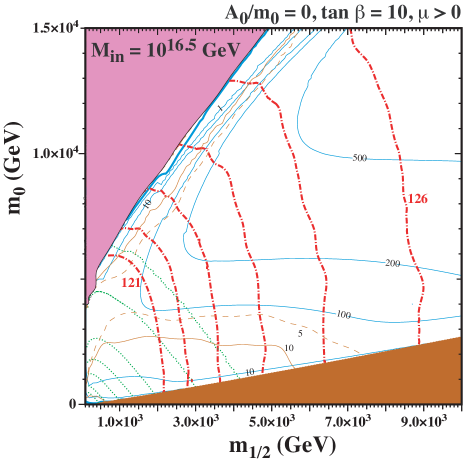
Figure 1: A representative $(m_{1/2},m_{0})$ plane in the flipped SU(5) GUT model, with $M_{in}=10^{16.5}$ GeV, $\tan\beta=10,A_{0}=0,\lambda_{4}=0.3,\lambda_{5}=0.1$ and $\lambda_{6}=0.0001$. Regions with a stau LSP and without electroweak symmetry breaking are shaded brown and pink, respectively. The red dot-dashed curves are contours of the Higgs mass from 121 - 126 GeV in intervals of 1 GeV, as calculated using FeynHiggs 2.18.1. The solid blue lines are contours of the relic density $\Omega_{LSP}h^{2}=0.1,1,10,100,200,500$. A thicker contour with $\Omega_{LSP}h^{2}=0.1$ is visible near the border of the no-electroweak symmetry breaking region, i.e., the focus-point region. The solid brown lines are where the central value of the $p\to e^{+}\pi^{0}$ lifetime is $10^{36}$ years (labelled 10 in units of $10^{35}$ years) and the dashed brown lines are where $\tau_{p}-\sigma_{\tau_{p}}=5\times 10^{35}$ years. The green dotted lines are contours of $\Delta a_{\mu}=1,2,5,10,20,50,100\times 10^{-11}$, increasing as $m_{1/2}$ and $m_{0}$ decrease.

The solid blue contours in Fig. 1 show values of the LSP relic density, $\Omega_{\chi}h^{2}$, as labeled, as calculated assuming that the Universe expands adiabatically. The contour for $\Omega_{\chi}h^{2}=0.1$, corresponding to the measured dark matter density, appears as a thick blue curve near the pale blue shaded area, and corresponds to the focus-point region [39]. There is also a short contour with $\Omega_{\chi}h^{2}=0.1$ just above the stau-LSP region with $m_{1/2}\lesssim 1$ TeV [40] that is almost invisible. As mentioned previously, the generation of a large amount ($\mathcal{O}(10^{4}$) ) of entropy in the early Universe due to the late decay of the flat direction responsible for the breaking of FSU(5) is a generic feature of FSU(5) cosmology [10, 11, 12, 16], so we do not interpret this adiabatic calculation of $\Omega_{\chi}h^{2}$ as a necessary constraint. Indeed when accounting for the late entropy production, we expect that parameters yielding $\Omega h^{2}\sim 100-1000$ would correspond better to the present relic density $\Omega h^{2}\simeq 0.1$. (See [41, 42] for related work.)

In addition, we show in Fig. 1 as the solid brown curve the contour where $\tau_{p}(p\to e^{+}\pi^{0})=10^{36}$ yrs, as calculated assuming normal ordering (NO) of the neutrino masses. This line appears at $m_{0}\approx 2.5$ TeV and also runs roughly parallel to the focus-point strip. The proton lifetime varies slowly across this plane, in general, and is always within the range 5 – 20 $\times 10^{35}$ yrs, beyond the foreseen experimental reach [23]. The brown dashed contour corresponds to $\tau_{p}-\sigma_{\tau_{p}}=5\times 10^{35}$ yrs, illustrating the effect of the uncertainty in the calculation of $\tau_{p}$ discussed in the previous Section.  Clearly, the relatively long proton lifetime in this plane makes detection difficult. Finally, we show a series of curves of constant $\Delta a_{\mu}$ as indicated in the caption, with the largest values appearing at small $m_{1/2}$ and $m_{0}$. We note that all values of $\Delta a_{\mu}>2\times 10^{-11}$ appear for values of $m_{h}<122$ GeV, outside the range that we consider compatible with the measured value of $m_{h}$.

In Fig. 2, we compare analogous planes with different values of $\tan\beta$. In the left panel, $\tan\beta=4$, while in the right panel $\tan\beta=35$. All other fixed parameters are the same as in Fig. 1. For $\tan\beta=4$, The Higgs mass is always less than 122 GeV, and only the $m_{h}=121$ GeV contour appears. The region without consistent electroweak symmetry breaking is pushed out beyond the range of the plot, so there is no visible focus-point region, and entropy production is required throughout the displayed plane. Compared to Fig. 1, the proton lifetime is longer and the values of $\Delta a_{\mu}$ are smaller for given values of $(m_{1/2},m_{0})$. In contrast, for the larger value of $\tan\beta=35$ shown in the right panel of Fig. 2, the region without electroweak symmetry breaking extends to lower values of $m_{1/2}$ and $m_{0}$, and the Higgs mass is higher, rising beyond 127 GeV in this plane. Though the proton lifetime is somewhat lower than in Fig. 2, it is still very large. On the other hand, values of $\Delta a_{\mu}$ are larger than in Fig. 2, and reach $10^{-10}$ for $m_{h}>122$ GeV.

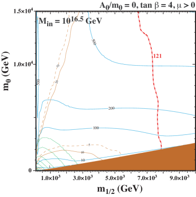
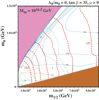
Figure 2: Representative $(m_{1/2},m_{0})$ planes in the FSU(5) GUT model. The parameters as the same as in Fig. 1 except that $\tan\beta=4$ in the left panel and $\tan\beta=35$ in the right panel. Regions with a stau LSP and without electroweak symmetry breaking are shaded brown and pink, respectively. The contours are as in Fig. 1, with the addition of contours for $\tau_{p}=2\times 10^{36}$ years and $\tau_{p}-\sigma_{\tau_{p}}=10^{36}$ years in the left panel.

We explore the dependence on $\lambda$ in Fig. 3. Keeping the other parameters fixed to the values used in Fig. 1, we take $\lambda$ = (0.1,0.3) in the upper left panel of Fig. 3, (0.3,0.3) (upper right), (0.3,0.5) (lower left), and (0.5,0.5) (lower right). None of the planes displays a constraint from electroweak symmetry breaking. This is tied to the larger value of $\lambda_{5}$ used here ($\geq 0.3$ vs the value of 0.1 used in Fig. 1). The Higgs mass and muon magnetic moment are relatively insensitive to $\lambda$. However, we see from Eq. (36) that the $X$ gauge boson mass is inversely proportional to $\sqrt{\lambda_{4}\lambda_{5}}$, so that increasing this product leads to a smaller mass and hence a shorter proton lifetime. Thus, whereas the lifetime for $\lambda$ = (0.1,0.3) is similar to the lifetime with (0.3,0.1), for $\lambda$ = (0.3,0.3) we see a mean lifetime contour of $5\times 10^{35}$ years and a 1$\sigma$-reduced lifetime of $2\times 10^{35}$ years running through the upper right panel. When the product $\sqrt{\lambda_{4}\lambda_{5}}$ is further increased, as in the lower left panel with $\lambda$ = (0.3,0.5), we see lifetime contours of 2, 5, and 10 $\times 10^{35}$ years, and reduced lifetime contours of 1, 2, and 5 $\times 10^{35}$ years. Finally, in the lower right panel with $\lambda$ = (0.5,0.5), we find proton lifetime contours of 1, 2, and 5 $\times 10^{35}$ years, and 1$\sigma$-reduced lifetimes of 0.5, 1, and 2 $\times 10^{35}$ years. We recall that lifetimes $\lesssim 10^{35}$ years open up the possibility of detection in the upcoming Hyper-Kamiokande experiment [23]. Finally, we note that higher values of $\lambda_{4,5}$ lead to problems in the running of the RGEs down from $M_{in}$ to $M_{GUT}$.

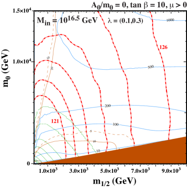
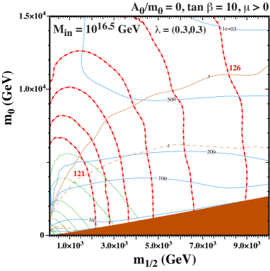
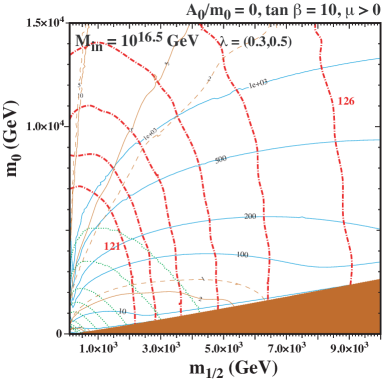
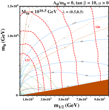
Figure 3: Representative $(m_{1/2},m_{0})$ planes in the FSU(5) GUT model. The fixed parameters as the same as in Fig. 1, except for $\lambda$ = (0.1,0.3) in the top left panel, $\lambda$ = (0.3,0.3) (top right), $\lambda$ = (0.3,0.5) (bottom left), and $\lambda$ = (0.5,0.5) (bottom right). Regions with a stau LSP are shaded brown. The contours are as in Fig. 1

The dependence on $M_{in}$ is considered in Fig. 4. The left panel assumes the same parameter values as in Fig. 1, with the exception of $M_{in}$, which is now set at the Planck scale. Electroweak symmetry breaking occurs throughout the plot, and the stau LSP region is pushed to the lower right corner of the panel. The Higgs mass, proton lifetime and relic density are all slightly larger than in Fig. 1. In the right panel, we again take $M_{in}=M_{P}$ but now with $\lambda$ = (0.3,0.3), which is near its upper limit for this value of $M_{in}$.

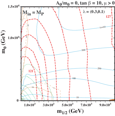
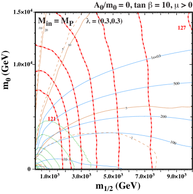
Figure 4: Representative $(m_{1/2},m_{0})$ planes in the FSU(5) GUT model. The fixed parameters as the same as in Fig. 1, except for $M_{in}=M_{P}$ and $\lambda$ = (0.3,0.1) in the left panel and $\lambda$ = (0.3,0.3) (right). The contours are as in Fig. 1.

The relation between the proton lifetime and $\sqrt{\lambda_{4}\lambda_{5}}$ is seen more clearly in Fig. 5, which shows a pair of $(\lambda_{4}=\lambda_{5},m_{0})$ planes for $m_{1/2}=5$ TeV, $A_{0}/m_{0}=0,\tan\beta=10$, $\mu>0$, $\lambda_{6}=0.0001$, with $M_{in}=10^{16.5}$ GeV (left panel) and $M_{in}=M_{P}$ (right panel). When $M_{in}=10^{16.5}$ GeV there is a small region in the upper left corner where electroweak symmetry breaking breaks down, which is shaded pink. Bordering this region, the focus-point strip with $\Omega h^{2}=0.1$ is the thick blue contour. Other blue contours correspond to larger values for the relic density, but we re-emphasize that larger values of $\Omega_{\chi}h^{2}$ would be allowed in the context of FSU(5) cosmology, in which substantial entropy is likely to have been generated in the early Universe. There is a stau LSP in the brown shaded region at low $m_{0}$ in the left panel. For $M_{in}=M_{P}$, the RGEs break down when $\lambda_{4}=\lambda_{5}\gtrsim 0.35$, as indicated by the red shading in the right panel. The red lines are contours of $m_{h}=125$ GeV. We note that $m_{h}$ varies slowly across this plane, so this is the only integer mass contour displayed. Finally, the solid brown lines are contours of $\tau(p\to e^{+}\pi^{0})$ in units of $10^{35}$ yrs. We see that values of the proton lifetime that are $\lesssim 3\times 10^{35}$ yrs, and hence potentially accessible to the next generation of experiment, are found in the right portions of the planes where $\lambda_{4}=\lambda_{5}\gtrsim 0.3$.

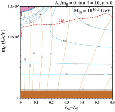
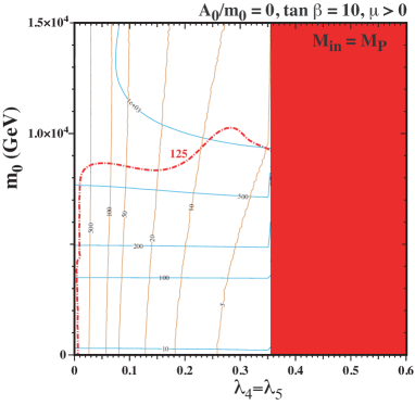
Figure 5: Representative $(\lambda_{4}=\lambda_{5},m_{0})$ planes in the FSU(5) GUT model with $M_{in}=10^{16.5}$ GeV ($M_{P}$) for the left (right) panel. The brown shaded region in the left panel is excluded because the LSP is charged, and there is no electroweak symmetry breaking in the pink shaded region, while the RGE equations break down in the red shaded band at large $\lambda_{4}=\lambda_{5}$ in the right panel. The contours are as in Fig. 1.

The parameter planes displayed above have all assumed $A_{0}=0$, and we present in Fig. 6 a pair of planes with non-zero $A_{0}$, specifically $A_{0}=3.8~{}m_{0}$. In the left panel, we take $M_{in}=10^{16.5}$ GeV and $\lambda$ = (0.5,0.5) to minimize the proton lifetime. In the right panel, $M_{in}=M_{P}$ and $\lambda$ = (0.3,0.3). These planes exhibit the possible importance of a compressed stop spectrum, which introduces the possibility of stop coannihilation [43], and can be compared with Fig. 12c of [16]. The brown shaded regions where $m_{0}>m_{1/2}$ are disallowed because the stop is either the LSP or tachyonic, and that in the left panel where $m_{1/2}>m_{0}$ has a stau LSP. As we have seen previously, the stau LSP region recedes to larger values of $m_{1/2}$ as $M_{in}$ increases, and is not visible in the right panel where $M_{in}=M_{P}$. We see very large values of $\Omega_{\chi}h^{2}$ in the bulk of the uncoloured region,  but there are strips close to the boundaries of the shaded regions where $\Omega_{\chi}h^{2}$ is reduced. Once again, the thick blue shaded contour running along the stop LSP region corresponds to $\Omega h^{2}=0.1$.

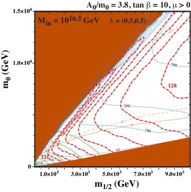
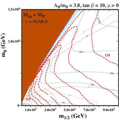
Figure 6: Representative $(m_{1/2},m_{0})$ planes in the FSU(5) GUT model. Parameters as in Fig. 1, except that $A_{0}/m_{0}=3.8$, $\lambda_{4}=\lambda_{5}=0.5$ (left), and $M_{in}=M_{P}$ with $\lambda_{4}=\lambda_{5}=0.3$, (right). Regions with a stau LSP, stop LSP or tachyonic stop/stau are shaded brown. The contours are as in Fig. 1.

It is important to note that we can find $\Omega h^{2}=0.1$ and $m_{h}=125$ GeV simultaneously in both panels in Fig. 6, but at very different values of $(m_{1/2},m_{0})$. For $M_{in}=10^{16.5}$ GeV, simultaneity occurs around $(m_{1/2},m_{0})\simeq(7,13)$ TeV where the proton lifetime $\tau_{p}\approx 5\pm 3\times 10^{35}$ years. However, for $M_{in}=M_{P}$, these conditions are both satisfied when $(m_{1/2},m_{0})\simeq(1.1,3.8)$ TeV.  Despite the lower sparticle masses, the proton lifetime is actually longer here (around $10^{36}$ years), mainly due to the lower values of $\lambda_{4,5}$ needed to ensure non-divergent running between $M_{P}$ and $M_{GUT}$. In both cases, the contribution to $\Delta a_{\mu}$ is small ($<10^{-11}$). We stress again, however, that as late-time entropy production is expected in this FSU(5) model, most of the displayed plane is viable cosmologically.

In Fig. 7, we show a pair of ($\lambda_{4,5},m_{0}$) planes with $A_{0}/m_{0}=3.8$ and $M_{in}=10^{16.5}$ GeV (left panel) and $M_{in}=M_{P}$ (right panel), as in Fig. 6. As previously, we see brown shaded regions where the lightest neutralino is not the LSP, and a red shaded region in the right panel where the RGEs break down. We again see stop strips. For the lower value of $M_{in}$, we choose $m_{1/2}=7$ TeV and for $M_{in}=M_{P}$, we take $m_{1/2}=2$ TeV. We find that $\Delta a_{\mu}$ is small everywhere in the left plane due to the large value of $m_{1/2}$, whereas in the right plane we see contours of $\Delta a_{\mu}=1$ and $2\times 10^{-11}$, also too small to make a significant contribution to resolving the discrepancy between experiment and the Standard Model calculation. As previously, we find that the proton lifetime is minimized, and potentially observable, for large $\lambda_{4}=\lambda_{5}$ and small $m_{0}$ when $M_{in}=10^{16.5}$ GeV, whereas the proton lifetime is generally longer when $M_{in}=M_{P}$.

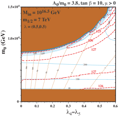
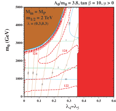
Figure 7: Representative ($\lambda_{4}=\lambda_{5},m_{0}$) planes in the FSU(5) GUT model, both with $A_{0}/m_{0}=3.8$. In the left panel $M_{in}=10^{16.5}$ GeV with $m_{1/2}=7$ TeV, whereas in the right panel $M_{in}=M_{P}$ with $m_{1/2}=2$ TeV. The brown shaded regions are excluded because the LSP is charged or tachyonic, and the RGEs break down in the red shaded region at large $\lambda_{4}=\lambda_{5}$ in the right panel. The contours are as in Fig. 1.

5.2 Non-Universal Models and $\mathbf{g_{\mu}-2}$

From the results in the previous subsection, it is clear that the contribution to $\Delta a_{\mu}$ is always small when universal boundary conditions applied for scalar and gaugino masses at $M_{in}$. Indeed, in all of the above planes, a significant contribution to $\Delta a_{\mu}$ occurs only at low supersymmetric masses that are in tension with LHC constraints and where the Higgs mass is well below the experimental value, even with a conservative assessment of the theoretical uncertainty in the calculation of $m_{h}$. On the other hand, previous analyses have shown that substantially larger contributions to $\Delta a_{\mu}$ are possible when some degree of universality is abandoned [20, 44].

Therefore, in this subsection, we depart from full gaugino and scalar mass universality at $M_{in}$, while retaining the constraints imposed by FSU(5). Thus, we include two independent gaugino masses, a common mass $M_{5}$ for the SU(5) gauginos $\tilde{g},\tilde{W}$ and $\tilde{B}$, and an independent mass $M_{X1}$ for the ‘external’ gaugino $\tilde{B}_{X}$. This is to be contrasted with our previous assumption that $M_{5}=M_{X1}=m_{1/2}$ at $M_{in}$. Similarly we now include five independent soft supersymmetry-breaking scalar masses, $m_{10}$ for sfermions in the $\mathbf{10}$ representations of SU(5), $m_{\bar{5}}$ for sfermions in the $\mathbf{\overline{5}}$ representations of SU(5), $m_{1}$ for the right-handed sleptons in the singlet representations, and two Higgs soft masses $m_{H_{u,d}}$ for the MSSM Higgs doublets stemming from $\mathbf{5}$ and $\mathbf{\overline{5}}$ representations of SU(5). Previously we had set $m_{10}=m_{\bar{5}}=m_{1}=m_{H_{u}}=m_{H_{d}}=m_{0}$. Guided by the results of [20], we make the illustrative choices $\tan\beta=35$, $A_{0}/m_{0}=1.8$, $M_{in}=10^{16.5}$ GeV, $M_{5}=2.4$ TeV, $m_{10}=1$ TeV, $m_{H_{d}}=-4.72$ TeV, and $m_{H_{u}}=-5.1$ TeV. For the latter two, the signs refer to the sign of mass-squared, and these choices correspond to the choice of $\mu=4.77$ TeV and a pseudo scalar mass, $m_{A}=2.1$ TeV for the example in [20]. These were found to optimize the value of $\Delta a_{\mu}$.

Some results are displayed in the $(M_{X1},m_{1})$ planes shown in Fig. 8. In the left panel, only the singlet masses $M_{X1}$ and $m_{1}$ break universality, i.e., we set $m_{\bar{5}}=m_{10}=1$ TeV in this case. The Higgs mass varies very little in this plane and is always slightly larger than 122 GeV (no contours are shown). Similarly the proton lifetime varies very little and is approximately $(1.2\pm 0.6)\times 10^{36}$ years. In contrast, the relic density (indicated by the labeled blue contours) varies significantly, reaching values as large as $\Omega h^{2}=500$ in the upper left corner of the panel. Also seen as vertical light blue lines are the lower limits to the mass of the lightest gaugino $m_{\chi}>100$ GeV (which is valid for generic slepton masses) and $>73$ GeV (which can be reached if the mass difference between the LSP and the lightest slepton $<2$ GeV). Finally, we show as green dotted lines some contours of $\Delta a_{\mu}$ in units of $10^{-11}$. In general, they are significantly larger than was found in the universal case, with contours of 10 and $15\times 10^{-11}$ appearing, the largest value of $\Delta a_{\mu}$ being $18\times 10^{-11}$. While an improvement over the universal case, these are still too small to account for the discrepancy between the Standard Model and experiment.

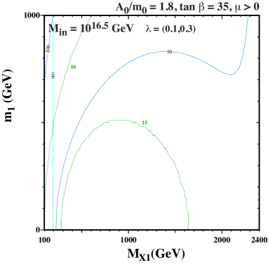
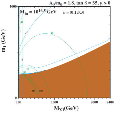
Figure 8: Some $(M_{X1},m_{1})$ planes in the FSU(5) GUT model with $M_{5}=2.4$ TeV, $m_{10}=1$ TeV, $\tan\beta=35$, $A_{0}/m_{10}=1.8$. We assume $m_{\bar{5}}=m_{10}$ in the left panel and $m_{\bar{5}}=m_{10}/2$ in the right panel. The contours are as in Fig. 1.

We can increase $\Delta a_{\mu}$ by choosing a lower value of $m_{\bar{5}}$ relative to $m_{10}$. As an example, in the right panel of Fig. 8 we take $m_{\bar{5}}=m_{10}/2$. The lower right portion of the figure, shaded brown, is excluded because the LSP is charged, namely the right-handed selectron/smuon. The $\Omega_{\chi}h^{2}=0.1$ contour appears along a selectron/smuon coannihilation strip running close to the boundary of the charged LSP region at small $m_{1}$. It is tracked by the $\Omega_{\chi}h^{2}=1$ contour at larger $m_{1}$. The Higgs mass values are similar to those in the left panel, varying very slowly and always about 122.3 GeV across the plane. The proton lifetime is also nearly constant at around $(1.1\pm 0.6)\times 10^{36}$ years. However, the contribution to $a_{\mu}$ is now significantly larger, as there are contours of 10 (in the upper left corner of the panel), 20, 50 and (in the lower left corner) 100, 150 and 200, again in units of $10^{-11}$. However, $\Delta a_{\mu}=200\times 10^{-11}$ appears outside the selectron/smuon LSP region only when the lightest gaugino mass is below its lower limit of 73 GeV. However, the $150\times 10^{-11}$ contour extends to the right of the vertical LSP mass limit of 100 GeV, in a region where the gaugino is the LSP and has a relic density $\Omega_{\chi}h^{2}\sim 0.1$. This region resembles the best $\Delta a_{\mu}$ point found in [20].

The sensitivity to $\lambda_{4,5}$ for similar choices of model parameters is shown in the left panel of Fig. 9, which displays a $(\lambda_{4,5},m_{1})$ plane with $M_{X1}=0.8$ TeV and other parameters the same as those used in the left panel of Fig. 8. In this case, we see only a single relic density contour, which has $\Omega_{\chi}h^{2}=10$. The Higgs mass is again slightly larger than 122 GeV across the plane, and $\Delta a_{\mu}\simeq(10-18)\times 10^{-11}$. However, we now see a large variation in the proton lifetime, which varies from $5\times 10^{37}$ years at low values of $\lambda_{4}=\lambda_{5}$, to $10^{35}$ years at large values.

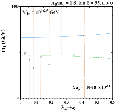
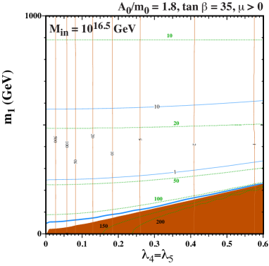
Figure 9: Representative $(\lambda_{4}=\lambda_{5},m_{1})$ planes in the FSU(5) GUT model. In both panels, $A_{0}/m_{0}=1.8$, $\tan\beta=35$ and $M_{in}=10^{16.5}$ GeV. In the left panel $M_{5}=2.4$ TeV, $M_{X1}=0.8$ TeV and $m_{10}=m_{\bar{5}}=1$ TeV, while in the right panel $M_{5}=2.4$ TeV, $M_{X1}=0.2$ TeV, $m_{10}=1$ TeV and $m_{\bar{5}}=0.5$ TeV. The contours are as in Fig. 1.

In contrast, in the right panel of Fig. 9 we fix $M_{X1}=200$ GeV, with $m_{10}=2m_{\bar{5}}=1$ TeV. The proton lifetime decreases as $\lambda_{4}=\lambda_{5}$ increase, becoming potentially observable for values $\gtrsim 0.4$ (taking into account the matrix element uncertainties). The Higgs mass is not very sensitive to the choice of $m_{\bar{5}}$ or the change in $M_{X1}$, with the Higgs mass being slightly above 122 GeV across the plane displayed. The relic density is decreased at low $m_{1}$, as the mass of the selectron is lower and there is now a long relic density selectron/smuon coannihilation strip where $\Omega h^{2}=0.1$ just above the brown shaded region where the LSP is a selectron or smuon. The value of $\Delta a_{\mu}$ is now larger as well, and we see contours of 10, 20, 50, $100\times 10^{-11}$ all lying above the selectron/smuon LSP region.  We note the appearance of a ‘quadrifecta’ strip at large $\lambda_{4}=\lambda_{5}$ close to the charged-LSP boundary, where $\Delta a_{\mu}\sim 100\times 10^{-11}$, $\tau(p\to e^{+}\pi^{0})$ is potentially detectable, $m_{h}$ is compatible with experiment and $\Omega_{\chi}h^{2}\sim 0.1$ (though the latter is not a requirement, as mentioned previously).

The sensitivities of the ‘quadrifecta’ region to some of the input parameters are shown in Fig. 10. In the upper pair of panels we explore the sensitivity to $A_{0}/m_{0}$, which is taken to be 1 and 3 in the left and right panels, respectively. We see that there is rather small sensitivity to $A_{0}/m_{0}$, with $\Delta a_{\mu}$ and the proton lifetime both increasing slightly with the value of $A_{0}/m_{0}$. In the lower pair of panels we explore the sensitivity to $\tan\beta$, which is taken to be 25 and 40 in the left and right panels, respectively. We see that $\Delta a_{\mu}$ is significantly smaller for $\tan\beta=25$ and larger for $\tan\beta=40$, whereas the proton lifetime is quite insensitive to $\tan\beta$. We recall that the validity of the perturbation regime is quite restricted for larger values of $\tan\beta$, and recall that our results are rather insensitive to the value of $\lambda_{6}$.

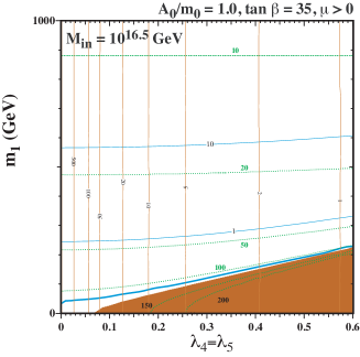
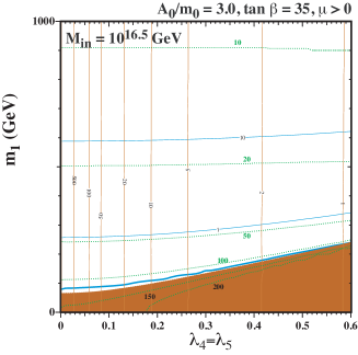
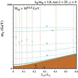
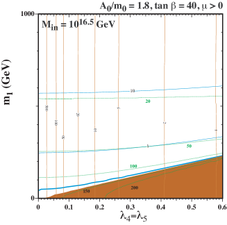
Figure 10: As in Fig. 9, but for different choices of $A_{0}/m_{0}=1,3$ (upper left and upper right panels) and of $\tan\beta=25,40$ (lower left and right panels). The contours are as in Fig. 1.

6 Conclusions

We have considered in this paper various aspects of the phenomenology of supersymmetric flipped SU(5) GUTs, focusing on predictions for proton decay and $g_{\mu}-2$. We have found that, if the soft supersymmetry-breaking parameters are constrained to be universal at some high scale $M_{in}$ above the GUT scale, the proton lifetime is typically $\gtrsim 10^{36}$ yrs and the supersymmetric contribution to $g_{\mu}-2$ is small. The proton lifetime is generally too long to be detected in the foreseeable future, and the model does not contribute significantly to reducing the tension between data-driven calculations of $g_{\mu}-2$ within the Standard Model and the experimental measurement. However, we have found that there is a region of the constrained flipped SU(5) parameter space with large $\mathbf{10\ 10\ 5}$ and $\mathbf{\overline{10}\ \overline{10}\ \overline{5}}$ couplings where $p\to e^{+}\pi^{0}$ decay may be detectable in the Hyper-Kamiokande experiment [23] now under construction. Nevertheless, the flipped SU(5) GUT contribution to $g_{\mu}-2$ is still small.

However, we have found that if the universality constraints on the soft supersymmetry-breaking masses are relaxed there is a region of flipped SU(5) GUT parameter space where the model contribution to $g_{\mu}-2$ can be large enough to reduce significantly the discrepancy between theory and experiment while $\tau(p\to e^{+}\pi^{0})$ may simultaneously be short enough to be detected in Hyper-Kamiokande. This region appears when $A_{0}/m_{0}\sim 1-3$ and $\tan\beta\sim 25-40$, for suitable values of the other flipped SU(5) parameters. We call this the ‘quadrifecta’ region, since the theoretical calculation of the light Higgs mass is compatible with the experimental measurement, within uncertainties, and the strip where the relic LSP density $\Omega_{\chi}h^{2}\simeq 0.12$ if the Universe expands adiabatically passes through the region. 

This ‘quadrifecta’ region was previously identified in a dedicated analysis of $g_{\mu}-2$ in the flipped SU(5) GUT [20], and it is encouraging that this region appears quite stable under mild variations in the input parameters. As pointed out in [20], in this region both the LSP and lighter smuon masses are very close to the LEP lower limits on their masses of $\sim 100$ GeV, and detection of the LSP, smuon and selectron should be possible at the LHC. Their discovery would be a striking success for the flipped SU(5) framework described here, which could be complemented by the detection of $p\to e^{+}\pi^{0}$ decay in the Hyper-Kamiokande experiment [23].

References

- [1] S. M. Barr, Phys. Lett. 112B (1982) 219; S. M. Barr, Phys. Rev. D 40, 2457 (1989).
- [2] J. P. Derendinger, J. E. Kim and D. V. Nanopoulos, Phys. Lett. 139B (1984) 170.
- [3] I. Antoniadis, J. R. Ellis, J. S. Hagelin and D. V. Nanopoulos, Phys. Lett. B 194 (1987) 231.
- [4] I. Antoniadis, J. R. Ellis, J. S. Hagelin and D. V. Nanopoulos, Phys. Lett. B 205 (1988) 459; Phys. Lett. B 208 (1988) 209 Addendum: [Phys. Lett. B 213 (1988) 562]; Phys. Lett. B 231 (1989) 65.
- [5] For a recent D-brane construction of flipped SU(5) and other references, see J. L. Lamborn, T. Li, J. A. Maxin and D. V. Nanopoulos, arXiv:2108.08084 [hep-ph].
- [6] J. Ellis, M. A. G. Garcia, N. Nagata, D. V. Nanopoulos and K. A. Olive, JHEP 05, 021 (2020) [arXiv:2003.03285 [hep-ph]].
- [7] M. Mehmood, M. U. Rehman and Q. Shafi, JHEP 02, 181 (2021) [arXiv:2010.01665 [hep-ph]].
- [8] N. Haba and T. Yamada, arXiv:2110.01198 [hep-ph].
- [9] J. R. Ellis, J. L. Lopez, D. V. Nanopoulos and K. A. Olive, Phys. Lett. B 308, 70 (1993) [hep-ph/9303307].
- [10] J. Ellis, M. A. G. Garcia, N. Nagata, D. V. Nanopoulos and K. A. Olive, JCAP 1707, no. 07, 006 (2017) [arXiv:1704.07331 [hep-ph]].
- [11] J. Ellis, M. A. G. Garcia, N. Nagata, D. V. Nanopoulos and K. A. Olive, JCAP 1904, no. 04, 009 (2019) [arXiv:1812.08184 [hep-ph]].
- [12] J. Ellis, M. A. G. Garcia, N. Nagata, D. V. Nanopoulos and K. A. Olive, Phys. Lett. B 797, 134864 (2019) [arXiv:1906.08483 [hep-ph]].
- [13] J. R. Ellis, J. S. Hagelin, S. Kelley, D. V. Nanopoulos and K. A. Olive, Phys. Lett. B 209, 283 (1988).
- [14] J. Ellis, A. Mustafayev and K. A. Olive, Eur. Phys. J. C 71, 1689 (2011) [arXiv:1103.5140 [hep-ph]].
- [15] B. A. Campbell, J. R. Ellis, J. S. Hagelin, D. V. Nanopoulos and K. A. Olive, Phys. Lett. B 197, 355 (1987); B. Campbell, J. R. Ellis, J. S. Hagelin, D. V. Nanopoulos and K. A. Olive, Phys. Lett. B 200, 483 (1988); J. R. Ellis, J. S. Hagelin, D. V. Nanopoulos and K. A. Olive, Phys. Lett. B 207, 451 (1988).
- [16] J. Ellis, M. A. G. Garcia, N. Nagata, D. V. Nanopoulos and K. A. Olive, JCAP 01 (2020), 035 [arXiv:1910.11755 [hep-ph]]; see also I. Antoniadis, D. V. Nanopoulos and J. Rizos, JCAP 03 (2021), 017 [arXiv:2011.09396 [hep-th]].
- [17] G. W. Bennett et al. [Muon g-2 Collaboration], Phys. Rev. D 73 (2006), 072003 [arXiv:hep-ex/0602035 [hep-ex]].
- [18] B. Abi et al. [Muon g-2 Collaboration] Phys. Rev. Lett. 126 (2021), 141801 [arXiv:2104.03281 [hep-ex]].
- [19] T. Aoyama, et al. Phys. Rept. 887 (2020), 1-166 [arXiv:2006.04822 [hep-ph]]; M. Davier, A. Hoecker, B. Malaescu and Z. Zhang, Eur. Phys. J. C 71 (2011), 1515 [erratum: Eur. Phys. J. C 72 (2012), 1874] [arXiv:1010.4180 [hep-ph]]; A. Kurz, T. Liu, P. Marquard and M. Steinhauser, Phys. Lett. B 734, 144-147 (2014) [arXiv:1403.6400 [hep-ph]]; M. Davier, A. Hoecker, B. Malaescu and Z. Zhang, Eur. Phys. J. C 77 (2017) no.12, 827 [arXiv:1706.09436 [hep-ph]]; A. Keshavarzi, D. Nomura and T. Teubner, Phys. Rev. D 97, no.11, 114025 (2018) [arXiv:1802.02995 [hep-ph]]; G. Colangelo, M. Hoferichter and P. Stoffer, JHEP 02, 006 (2019) [arXiv:1810.00007 [hep-ph]]; M. Hoferichter, B. L. Hoid and B. Kubis, JHEP 08, 137 (2019) [arXiv:1907.01556 [hep-ph]]; M. Davier, A. Hoecker, B. Malaescu and Z. Zhang, Eur. Phys. J. C 80 (2020) no.3, 241 [erratum: Eur. Phys. J. C 80 (2020) no.5, 410] [arXiv:1908.00921 [hep-ph]]; A. Keshavarzi, D. Nomura and T. Teubner, Phys. Rev. D 101, no.1, 014029 (2020) [arXiv:1911.00367 [hep-ph]].
- [20] J. Ellis, J. L. Evans, N. Nagata, D. V. Nanopoulos and K. A. Olive, arXiv:2107.03025 [hep-ph].
- [21] S. Borsanyi, Z. Fodor, J. N. Guenther, C. Hoelbling, S. D. Katz, L. Lellouch, T. Lippert, K. Miura, L. Parato and K. K. Szabo, et al. Nature 593 (2021) no.7857, 51-55 doi:10.1038/s41586-021-03418-1 [arXiv:2002.12347 [hep-lat]].
- [22] T. Li, J. A. Maxin and D. V. Nanopoulos, arXiv:2107.12843 [hep-ph].
- [23] K. Abe et al. [Hyper-Kamiokande Collaboration], arXiv:1805.04163 [physics.ins-det].
- [24] Y. Aoki, T. Izubuchi, E. Shintani and A. Soni, Phys. Rev. D 96 (2017) no.1, 014506 [arXiv:1705.01338 [hep-lat]].
- [25] J. Ellis, J. L. Evans, N. Nagata, K. A. Olive and L. Velasco-Sevilla, Eur. Phys. J. C 80 (2020) no.4, 332 [arXiv:1912.04888 [hep-ph]].
- [26] L. Calibbi, Y. Mambrini and S. K. Vempati, JHEP 0709, 081 (2007) [arXiv:0704.3518 [hep-ph]]; L. Calibbi, A. Faccia, A. Masiero and S. K. Vempati, Phys. Rev. D 74, 116002 (2006) [arXiv:hep-ph/0605139]; E. Carquin, J. Ellis, M. E. Gomez, S. Lola and J. Rodriguez-Quintero, JHEP 0905 (2009) 026 [arXiv:0812.4243 [hep-ph]].
- [27] J. Ellis, A. Mustafayev and K. A. Olive, Eur. Phys. J. C 69, 201 (2010) [arXiv:1003.3677 [hep-ph]]; J. Ellis, A. Mustafayev and K. A. Olive, Eur. Phys. J. C 69, 219-233 (2010) [arXiv:1004.5399 [hep-ph]].
- [28] J. Ellis, K. Olive and L. Velasco-Sevilla, Eur. Phys. J. C 76, no.10, 562 (2016) [arXiv:1605.01398 [hep-ph]]; J. Ellis, J. L. Evans, N. Nagata, K. A. Olive and L. Velasco-Sevilla, Eur. Phys. J. C 81, no.2, 120 (2021) [arXiv:2011.03554 [hep-ph]].
- [29] J. Ellis, J. L. Evans, A. Mustafayev, N. Nagata and K. A. Olive, Eur. Phys. J. C 76, no.11, 592 (2016) [arXiv:1608.05370 [hep-ph]].
- [30] J. Ellis, J. L. Evans, N. Nagata, D. V. Nanopoulos and K. A. Olive, Eur. Phys. J. C 77, no.4, 232 (2017) [arXiv:1702.00379 [hep-ph]].
- [31] P. A. Zyla et al. [Particle Data Group], PTEP 2020 (2020) no.8, 083C01.
- [32] J. Ellis, M. A. G. Garcia, N. Nagata, D. V. Nanopoulos, K. A. Olive and S. Verner, Int. J. Mod. Phys. D 29, no.16, 2030011 (2020) [arXiv:2009.01709 [hep-ph]].
- [33] J. Ellis, K. Olive and Y. Santoso, Phys. Lett. B 539 (2002) 107 [arXiv:hep-ph/0204192]; J. R. Ellis, T. Falk, K. A. Olive and Y. Santoso, Nucl. Phys. B 652 (2003) 259 [arXiv:hep-ph/0210205].
- [34] S. Heinemeyer, W. Hollik and G. Weiglein, Comput. Phys. Commun. 124 (2000) 76 [arXiv:hep-ph/9812320]; S. Heinemeyer, W. Hollik and G. Weiglein, Eur. Phys. J. C 9 (1999) 343 [arXiv:hep-ph/9812472]; G. Degrassi, S. Heinemeyer, W. Hollik, P. Slavich and G. Weiglein, Eur. Phys. J. C 28 (2003) 133 [arXiv:hep-ph/0212020]; M. Frank et al., JHEP 0702 (2007) 047 [arXiv:hep-ph/0611326]; T. Hahn, S. Heinemeyer, W. Hollik, H. Rzehak and G. Weiglein, Comput. Phys. Commun. 180 (2009) 1426; T. Hahn, S. Heinemeyer, W. Hollik, H. Rzehak and G. Weiglein, Phys. Rev. Lett. 112 (2014) 14, 141801 [arXiv:1312.4937 [hep-ph]]; H. Bahl and W. Hollik, Eur. Phys. J. C 76 (2016) no.9, 499 [arXiv:1608.01880 [hep-ph]]; H. Bahl, S. Heinemeyer, W. Hollik and G. Weiglein, Eur. Phys. J. C 78 (2018) no.1, 57 [arXiv:1706.00346 [hep-ph]]. H. Bahl, T. Hahn, S. Heinemeyer, W. Hollik, S. Passehr, H. Rzehak and G. Weiglein, Comput. Phys. Commun. 249 (2020) 107099 [arXiv:1811.09073 [hep-ph]]. See http://www.feynhiggs.de for updates.
- [35] K. Hamaguchi, S. Hor and N. Nagata, JHEP 11, 140 (2020) [arXiv:2008.08940 [hep-ph]].
- [36] C. Munoz, Phys. Lett. B 177, 55 (1986).
- [37] L. F. Abbott and M. B. Wise, Phys. Rev. D 22, 2208 (1980).
- [38] T. Nihei and J. Arafune, Prog. Theor. Phys. 93, 665 (1995) [hep-ph/9412325].
- [39] J. L. Feng, K. T. Matchev and T. Moroi, Phys. Rev. Lett. 84, 2322 (2000) [arXiv:hep-ph/9908309]; H. Baer, T. Krupovnickas, S. Profumo and P. Ullio, JHEP 0510 (2005) 020 [hep-ph/0507282]; J. L. Feng, K. T. Matchev and D. Sanford, Phys. Rev. D 85, 075007 (2012) [arXiv:1112.3021 [hep-ph]]; P. Draper, J. Feng, P. Kant, S. Profumo and D. Sanford, Phys. Rev. D 88, 015025 (2013) [arXiv:1304.1159 [hep-ph]].
- [40] J. Ellis, T. Falk, and K.A. Olive, Phys. Lett. B444 (1998) 367 [arXiv:hep-ph/9810360]; J. Ellis, T. Falk, K.A. Olive, and M. Srednicki, Astr. Part. Phys. 13 (2000) 181 [Erratum-ibid. 15 (2001) 413] [arXiv:hep-ph/9905481]; M. Citron, J. Ellis, F. Luo, J. Marrouche, K. A. Olive and K. J. de Vries, Phys. Rev. D 87, no. 3, 036012 (2013) [arXiv:1212.2886 [hep-ph]], and references therein; N. Desai, J. Ellis, F. Luo and J. Marrouche, Phys. Rev. D 90, no. 5, 055031 (2014) [arXiv:1404.5061 [hep-ph]].
- [41] J. T. Giblin, G. Kane, E. Nesbit, S. Watson and Y. Zhao, Phys. Rev. D 96, no.4, 043525 (2017) [arXiv:1706.08536 [hep-th]].
- [42] R. Allahverdi and J. K. Osiński, [arXiv:2108.13136 [hep-ph]].
- [43] C. Boehm, A. Djouadi and M. Drees, Phys. Rev. D 62, 035012 (2000) [arXiv:hep-ph/9911496]; J. R. Ellis, K. A. Olive and Y. Santoso, Astropart. Phys. 18, 395 (2003) [arXiv:hep-ph/0112113]; J. L. Diaz-Cruz, J. R. Ellis, K. A. Olive and Y. Santoso, JHEP 0705, 003 (2007) [arXiv:hep-ph/0701229]; I. Gogoladze, S. Raza and Q. Shafi, Phys. Lett. B 706, 345 (2012) [arXiv:1104.3566 [hep-ph]]; M. A. Ajaib, T. Li and Q. Shafi, Phys. Rev. D 85, 055021 (2012) [arXiv:1111.4467 [hep-ph]]; J. Harz, B. Herrmann, M. Klasen, K. Kovarik and Q. L. Boulc’h, Phys. Rev. D 87 (2013) 5, 054031 [arXiv:1212.5241]; J. Harz, B. Herrmann, M. Klasen and K. Kovarik, Phys. Rev. D 91 (2015) 3, 034028 [arXiv:1409.2898 [hep-ph]]; A. Ibarra, A. Pierce, N. R. Shah and S. Vogl, Phys. Rev. D 91, no. 9, 095018 (2015) [arXiv:1501.03164 [hep-ph]].
- [44] A. K. Forster and S. F. King, arXiv:2109.10802 [hep-ph].