Reactor antineutrino anomaly in light of recent flux model refinements

Abstract

We study the status of the reactor antineutrino anomaly in light of recent reactor flux models obtained with the conversion and summation methods. We present a new improved calculation of the IBD yields of the standard Huber-Mueller (HM) model and those of the new models. We show that the reactor rates and the fuel evolution data are consistent with the predictions of the Kurchatov Institute (KI) conversion model and with those of the Estienne-Fallot (EF) summation model, leading to a plausible robust demise of the reactor antineutrino anomaly. We show that the results of several goodness of fit tests favor the KI and EF models over other models that we considered. We also discuss the implications of the new reactor flux models for short-baseline neutrino oscillations due to active-sterile mixing. We show that reactor data give upper bounds on active-sterile neutrino mixing that are not very different for the reactor flux models under consideration and are in tension with the large mixing required by the Gallium anomaly that has been refreshed by the recent results of the BEST experiment.

I Introduction

Electron antineutrinos from nuclear reactors have been widely used to study the fundamental properties of neutrinos [1]. Reactor antineutrinos are produced from beta decays of neutron-rich fission fragments generated by the heavy fissionable isotopes ${}^{235}\text{U}$, ${}^{238}\text{U}$, ${}^{239}\text{Pu}$, and ${}^{241}\text{Pu}$ (see the reviews in Refs. [2, 3, 4]). Nuclear reactors are divided in two types: research reactors with nuclear fuel made of practically pure ${}^{235}\text{U}$ and commercial reactors that have typical fuel compositions that are dominated by ${}^{235}\text{U}$ ($\sim 50-60\%$) and ${}^{239}\text{Pu}$ ($\sim 25-35\%$), with small amounts of ${}^{238}\text{U}$ ($\lesssim 8\%$) and ${}^{241}\text{Pu}$ ($\lesssim 6\%$). Therefore, the most important antineutrino fluxes are those produced by the fissions of ${}^{235}\text{U}$ and ${}^{239}\text{Pu}$.

The antineutrino fluxes produced by the four fissionable isotopes have been calculated several times since the discovery of neutrinos in the reactor Cowan and Reines experiment [5] (see, for example, Ref. [6] and references therein). In 2011 new calculations by Mueller et al. [7] and Huber [8] (HM model) predicted reactor antineutrino fluxes that are about 5% larger than previous estimations and larger than the fluxes measured in several short-baseline reactor neutrino experiments with different fission fractions and different baselines. This discrepancy is known as the “reactor antineutrino anomaly” (RAA) [9].

The calculations of the reactor antineutrino fluxes are based on two methods: the summation method and the conversion method (see the reviews in Refs [3, 4]). The summation method (sometimes called ab initio) uses the fission fraction and $\beta$-decay information in nuclear databases to calculate the contribution of each single branch of the $\beta$-decay chains. Since nuclear databases are incomplete and sometimes inaccurate, the inferred reactor antineutrino spectra have potentially large and unknown uncertainties. In the conversion method the ${}^{235}\text{U}$, ${}^{239}\text{Pu}$, and ${}^{241}\text{Pu}$ antineutrino spectra are inferred from the corresponding $\beta$ spectra measured in the 1980’s at the Institut Laue-Langevin (ILL) [10, 11, 12]. The converted ${}^{238}\text{U}$ antineutrino spectrum was obtained in 2013 from the $\beta$ spectrum measured by an experiment at the scientific neutron source FRM II in Garching [13]. The conversion method was considered as more reliable and with small uncertainties (about 2-3%; see Refs. [2, 14]) before the discovery of the so-called “5 MeV bump” in 2014 (see the reviews in Refs [3, 4]) in the RENO [15], Double Chooz [16], and Daya Bay [17] experiments.

Mueller et al. [7] first used the summation method to obtain the antineutrino spectra of ${}^{235}\text{U}$, ${}^{238}\text{U}$, ${}^{239}\text{Pu}$ and ${}^{241}\text{Pu}$. In a second step, they corrected the ${}^{235}\text{U}$, ${}^{239}\text{Pu}$ and ${}^{241}\text{Pu}$ spectra adding the missing contributions obtained from the conversion of the ILL $\beta$-spectra [11, 10, 12]. These spectra were further corrected with an improved conversion method by Huber [8]. Therefore, in the HM model the ${}^{235}\text{U}$, ${}^{239}\text{Pu}$ and ${}^{241}\text{Pu}$ antineutrino spectra are those obtained by Huber [8] with the conversion method and the ${}^{238}\text{U}$ antineutrino spectrum is that obtained by Mueller et al. [7] with the summation method.

Nuclear databases have been improved in recent years, especially through the application of the Total Absorption Gamma-ray Spectroscopy (TAGS) technique for a better identification of the $\beta$ decay branches. In 2019 Estienne, Fallot et al [18] (EF model), using updated nuclear database information, obtained a ${}^{235}\text{U}$ reactor antineutrino flux that is smaller than that of the HM model and roughly in agreement with the experimental measurements. A similar result has been obtained in Ref. [19]. If these predictions describe correctly the real reactor antineutrino fluxes, the reactor antineutrino anomaly disappears. Let us however note that low predictions of the reactor antineutrino fluxes with the summation method may be due to residual incompleteness of the nuclear database that is used in the calculation. Moreover, it has been shown that the analytical approximation of the single beta spectrum using the Fermi function and additional corrections may induce a reactor spectral variation at the level of 2% with the summation method [20]. The EF fluxes give a better fit of the Daya Bay antineutrino spectrum [21] than the HM fluxes, but they give a worse fit of the 5 MeV bump. Therefore, it is uncertain if the EF fluxes are more reliable than the HM fluxes.

An opposite result concerning the reactor antineutrino anomaly is obtained by using the 2019 calculation of the reactor antineutrino fluxes in Ref. [22] (HKSS model) using the conversion method. The authors of this paper improved the conversion method by considering forbidden transitions calculated with the nuclear shell model, that give a partial explanation of the 5 MeV bump. The resulting antineutrino fluxes are larger than those of the HM model and lead to an increase of the reactor antineutrino anomaly. Note that also another conversion calculation [23] found that taking account the forbidden transitions could partially explain the bump feature and result in a larger flux anomaly.

More recently, in the beginning of 2021, Kopeikin et al. [24] corrected the ${}^{235}\text{U}$ $\beta$ spectrum measured at ILL [10, 11] using new relative measurements of the ratio of the ${}^{235}\text{U}$ and ${}^{239}\text{Pu}$ $\beta$ spectra performed with a research reactor at the Kurchatov Institute (KI model). These measurements show an excess of the ILL ratio of the ${}^{235}\text{U}$ and ${}^{239}\text{Pu}$ $\beta$ spectra by a factor $1.054\pm 0.002$. Kopeikin et al. argued that it is likely that the normalization of the ILL ${}^{235}\text{U}$ $\beta$ spectrum was overestimated. Therefore, the KI model predicts a converted ${}^{235}\text{U}$ antineutrino flux that is smaller than that in the HM model and converted ${}^{239}\text{Pu}$ and ${}^{241}\text{Pu}$ antineutrino fluxes that are similar to those of the HM model. For the ${}^{238}\text{U}$ antineutrino flux, Kopeikin et al. applied the conversion method to the Garching ${}^{238}\text{U}$ $\beta$ spectrum [13], revising the normalization of the Garching ${}^{238}\text{U}$ $\beta$ spectrum to the ILL ${}^{235}\text{U}$ spectrum. The resulting ${}^{238}\text{U}$ antineutrino flux is slightly smaller than that in the HM model. In total, the KI model predicts antineutrino rates in short-baseline reactor experiments that are smaller than those predicted by the HM model and in approximate agreement with the EF predictions, hinting for a demise of the reactor antineutrino anomaly.

In this paper we consider, besides the HM, EF, HKSS and KI models, also a model that we call “HKSS-KI”, that is a modification of the HKSS model that we calculated taking into account the KI correction to the normalization of the ${}^{235}\text{U}$ antineutrino flux. Considering this hybrid model is justified by the interesting better fit of the 5 MeV bump in the HKSS model with respect to the HM model due to the inclusion of forbidden transitions (see the discussion in Section VIII.A of Ref. [22]).

The reduction of the ${}^{235}\text{U}$ antineutrino flux in the KI model with respect to the HM model is in agreement with the indications obtained by the measurements of the evolution of the antineutrino detection rate with the fuel composition in the Daya Bay [25, 26] and RENO [27] experiments, with the confirmation of a suppression of the ${}^{235}\text{U}$ antineutrino flux with respect to the HM model found in the recent PROSPECT [28, 29] and STEREO [30, 29] experiments at research reactors with practically pure ${}^{235}\text{U}$ fuel, and with the summation calculations in Refs. [18, 19] (see also the discussions in Refs. [31, 32, 33, 34, 35, 36, 37]). Let us however note that the KI suppression of the ratio of the ${}^{235}\text{U}$ and ${}^{239}\text{Pu}$ $\beta$ spectra with respect to the ILL measurements is not certain, at least until it is confirmed by another independent experiment. Moreover, it could also be explained with an enhancement of the ${}^{239}\text{Pu}$ $\beta$ spectrum, that would lead to a ${}^{239}\text{Pu}$ antineutrino flux higher than that in the HM model, with an enhancement of the reactor antineutrino anomaly. It is interesting that fits of the reactor data that include neutrino oscillations do not disfavor this possibility [34, 36].

Neutrino oscillations can explain the reactor antineutrino anomaly if there is at least one non-standard neutrino with a mass of the order of 1 eV or larger. These non-standard massive neutrinos must be mainly sterile, in order to preserve the well-established neutrino oscillation explanation of the data of solar, atmospheric and long-baseline neutrino oscillation experiments (see the reviews in Refs. [38, 39, 40, 41, 42]). In this case, a suppression of the rate measured in short-baseline reactor neutrino experiments with respect to the theoretical prediction is due to the disappearance of active $\bar{\nu}_{e}$’s. This mechanism can be distinguished from an explanation of the reactor antineutrino anomaly based on a suppression of the production of one or more of the four fluxes (mainly the dominant ${}^{235}\text{U}$ flux) through the following two important features: A) it acts in an equal way on the four fluxes; B) it has an oscillatory dependence on the distance $L$ from the reactor to the detector. Here we consider the simplest 3+1 model, with an effective mixing of the three standard neutrinos with one non-standard neutrino $\nu_{4}$ with a mass of the order of 1 eV or larger. In this model, the effective short-baseline survival probability of electron neutrinos and antineutrinos is given by

$$P_{ee}\simeq 1-\sin^{2}2\vartheta_{ee}\,\sin^{2}\left(\frac{\Delta m_{41}^{2}L}{4E}\right),$$ (1)

where $\Delta m_{41}^{2}=m_{4}^{2}-m_{1}^{2}\gtrsim 1\,\text{eV}^{2}$ is the squared-mass splitting between the non-standard massive neutrino $\nu_{4}$ and the three standard massive neutrinos $\nu_{1}$, $\nu_{2}$, $\nu_{3}$ that have lighter masses with the much smaller solar and atmospheric squared-mass splittings $\Delta m_{21}^{2}\approx 7.4\times 10^{-5}\,\text{eV}^{2}$ and $|\Delta m_{31}^{2}|\approx 2.5\times 10^{-3}\,\text{eV}^{2}$ (see Ref. [1] and the recent three-neutrino global analyses in Refs. [43, 44, 45]). The effective mixing angle $\vartheta_{ee}$ depends on the element $U_{e4}$ of the $4\times 4$ mixing matrix $U$ through the relation $\sin^{2}2\vartheta_{ee}=4|U_{e4}|^{2}(1-|U_{e4}|^{2})$.

The goal of this paper is to compare the fits of the reactor rate and fuel evolution data with the HM, EF, HKSS, KI and HKSS-KI models, to assess the status of the reactor antineutrino anomaly and short-baseline oscillations generated by a sterile neutrino at the eV mass scale. As far as we know there is not an established deviation from a standard value that defines an anomaly. For the discussion, we will consider as anomalous a deviation larger than $2\sigma$. However, this value is not very large, corresponding to a probability of about 5% of a type-I error, that is not very safe. Therefore, the statement that there is an anomaly must be weighted by the number of $\sigma$’s.

This paper is organized as follows. In Section II we present the results of a new improved calculation of the predictions of the HM, EF, HKSS, KI and HKSS-KI models. In Section III we discuss the method of analysis of the reactor antineutrino data. In Sections IV and V we present, respectively, the results of the fits of the reactor rates and the Daya Bay and RENO evolution data. In Section VI we discuss how to select the best-fit reactor flux model. In Section VII we discuss the implications for neutrino oscillations. Finally, the concluding remarks are presented in Section VIII.

II Model predictions

The event rate measured in reactor neutrino experiments can be expressed in a convenient way as a “cross section per fission” $\sigma_{f,a}$, often called “inverse beta decay (IBD) yield”:

$$\sigma_{f,a}=\sum_{i}f_{i}^{a}\sigma_{i},$$ (2)

where $a$ is the experiment label, $\sigma_{i}$ is the IBD yield for the fissionable isotope $i$ (with $i=235$, $238$, $239$, and $241$ for ${}^{235}\text{U}$, ${}^{238}\text{U}$, ${}^{239}\text{Pu}$, and ${}^{241}\text{Pu}$, respectively), and $f_{i}^{a}$ is the effective fission fraction of the isotope $i$ for the experiment $a$. For each fissionable isotope $i$, the individual IBD yield is given by

$$\sigma_{i}=\int_{E_{\nu}^{\text{thr}}}^{E_{\nu}^{\text{max}}}dE_{\nu}\,\Phi_{i}(E_{\nu})\,\sigma_{\text{IBD}}(E_{\nu}),$$ (3)

where $E_{\nu}$ is the neutrino energy, $\Phi_{i}(E_{\nu})$ is the neutrino flux generated by the fissionable isotope $i$, and $\sigma_{\text{IBD}}(E_{\nu})$ is the detection cross section. The neutrino energy is integrated from the threshold energy $E_{\nu}^{\text{thr}}=1.806\,\text{MeV}$ to a maximum value $E_{\nu}^{\text{max}}\geq 8\,\text{MeV}$. The numerical values of the $\sigma_{i}$’s predicted by a theoretical model depend on the way in which the integral in Eq. (3) is performed, taking into account that the neutrino fluxes are given in tabulated bins.

Model	$\bm{\sigma_{235}}$	$\bm{\sigma_{238}}$	$\bm{\sigma_{239}}$	$\bm{\sigma_{241}}$
HM	$6.69\pm 0.14$	$10.10\pm 0.82$	$4.40\pm 0.11$	$6.03\pm 0.13$
EF	$6.28\pm 0.31$	$10.14\pm 1.01$	$4.42\pm 0.22$	$6.23\pm 0.31$
HKSS	$6.74\pm 0.17$	$10.33\pm 0.85$	$4.43\pm 0.13$	$6.07\pm 0.16$
KI	$6.27\pm 0.13$	$9.34\pm 0.47$	$4.33\pm 0.11$	$6.01\pm 0.13$

Table 1: The original theoretical IBD yields of the four fissionable isotopes in units of $10^{-43}\text{cm}^{2}/\text{fission}$ predicted by the HM [7, 9, 8, 46], EF [18], HKSS [22], and KI [24] models.

Model	$\bm{\sigma_{235}}$	$\bm{\sigma_{238}}$	$\bm{\sigma_{239}}$	$\bm{\sigma_{241}}$
HM	$6.60\pm 0.14$	$10.00\pm 1.12$	$4.33\pm 0.11$	$6.01\pm 0.13$
EF	$6.17\pm 0.13$	$9.94\pm 1.09$	$4.32\pm 0.11$	$6.10\pm 0.13$
HKSS	$6.67\pm 0.15$	$10.08\pm 1.14$	$4.37\pm 0.12$	$6.06\pm 0.14$

Table 2: The theoretical IBD yields of the four fissionable isotopes in units of $10^{-43}\text{cm}^{2}/\text{fission}$ recalculated in Ref. [37] for the HM, EF, and HKSS models.

Model	$\bm{\sigma_{235}}$	$\bm{\sigma_{238}}$	$\bm{\sigma_{239}}$	$\bm{\sigma_{241}}$
HM	$6.74\pm 0.17$	$10.19\pm 0.83$	$4.40\pm 0.13$	$6.10\pm 0.16$
EF	$6.29\pm 0.31$	$10.16\pm 1.02$	$4.42\pm 0.22$	$6.23\pm 0.31$
HKSS	$6.82\pm 0.18$	$10.28\pm 0.84$	$4.45\pm 0.13$	$6.17\pm 0.16$
KI	$6.41\pm 0.14$	$9.53\pm 0.48$	$4.40\pm 0.13$	$6.10\pm 0.16$
HKSS-KI	$6.48\pm 0.14$	$10.28\pm 0.84$	$4.45\pm 0.13$	$6.17\pm 0.16$

Table 3: Our estimations of the theoretical IBD yields of the four fissionable isotopes in units of $10^{-43}\text{cm}^{2}/\text{fission}$ predicted by different models.

Table 3 gives the original theoretical IBD yields of the four fissionable isotopes predicted by the HM [7, 9, 8, 46], EF [18], HKSS [22], and KI [24] models. Since the uncertainties of the EF model are not given in Ref. [18], we considered the uncertainties associated with the summation spectra estimated in Ref. [33]: 5% for ${}^{235}\text{U}$, ${}^{239}\text{Pu}$, and ${}^{241}\text{Pu}$, and 10% for ${}^{238}\text{U}$.

The HM, EF, and HKSS predictions have been recently recalculated in Ref. [37], with some differences in the interpolation of the tabulated neutrino fluxes, the detection cross section, and considering $E_{\nu}^{\text{max}}=8\text{MeV}$. The resulting IBD yields shown in Table 3 are slightly smaller than the corresponding original IBD yields in Table 3. The uncertainties are similar, except for the uncertainties of $\sigma_{235}$, $\sigma_{239}$, and $\sigma_{241}$ in the EF model, for which the authors of Ref. [37] adopted the relative systematic uncertainties of the HM model. We do not agree with this choice, since the conversion and summation methods have different uncertainties. We think that the systematic uncertainties of the values of $\sigma_{235}$, $\sigma_{239}$, and $\sigma_{241}$ obtained with the conversion method in the HM model underestimate the corresponding uncertainties of the summation method following from the incomplete information in the nuclear databases.

Taking into account that an accurate estimation of the IBD yields and their uncertainties is crucial for a reliable assessment of the reactor antineutrino anomaly, we performed a new calculation for each of the different models. The results are presented in Table 3.

For all models, we calculated the IBD yields in Eq. (3) using the Strumia and Vissani IBD cross section [47], that improved the often-used Vogel and Beacom IBD cross section [48]. Historically, the reference IBD cross section is that in the famous 1971 review of Llewellyn Smith [49], which neglected contributions of order $(m_{n}-m_{p})/E_{\nu}$, that is not small for reactor neutrinos near the neutrino energy threshold, since $m_{n}-m_{p}=1.293\,\text{MeV}$ ($m_{n}$ and $m_{p}$ are, respectively, the neutron and proton masses). The Vogel and Beacom IBD cross section [48] considers these contributions, but it was calculated at first order in $E_{\nu}/m_{p}$. This is a good approximation for most calculations concerning reactor neutrinos, for which $E_{\nu}/m_{p}\lesssim 10^{-2}$. However, since the RAA is an effect of a few percent, it is better to use the more precise Strumia and Vissani IBD cross section [47] that was calculated without any approximation concerning $E_{\nu}/m_{p}$ and $(m_{n}-m_{p})/E_{\nu}$. In the implementation of the Strumia and Vissani formula for the IBD cross section, we considered the PDG 2020 [1] updated values of all the parameters. We also considered the radiative corrections calculated in Ref. [50], that are well approximated by Eq. (14) of Ref. [47].

$a$	Experiment	$f^{a}_{235}$	$f^{a}_{238}$	$f^{a}_{239}$	$f^{a}_{241}$	$\sigma_{f,a}^{\text{exp}}$	$R_{a,\text{HM}}^{\text{exp}}$	$R_{a,\text{EF}}^{\text{exp}}$	$R_{a,\text{HKSS}}^{\text{exp}}$	$R_{a,\text{KI}}^{\text{exp}}$	$R_{a,\text{HKSS-KI}}^{\text{exp}}$	$\delta_{a}^{\text{exp}}$ [%]	$\delta_{a}^{\text{cor}}$ [%]	$L_{a}$ [m]
$1$

& $0.538$ $0.078$ $0.328$ $0.056$ $5.75$ $0.927$ $0.962$ $0.916$ $0.962$ $0.944$ $1.4$ }220pt[1.4] $15$ $2$ Rovno91 $0.614$ $0.074$ $0.274$ $0.038$ $5.85$ $0.924$ $0.965$ $0.914$ $0.962$ $0.945$ $2.8$

$18$ $3$ Rovno88-1I $0.607$ $0.074$ $0.277$ $0.042$ $5.70$ $0.902$ $0.941$ $0.892$ $0.939$ $0.921$ $6.4$ }220pt[3.1] }520pt[2.2] $18$ $4$ Rovno88-2I $0.603$ $0.076$ $0.276$ $0.045$ $5.89$ $0.931$ $0.971$ $0.920$ $0.969$ $0.951$ $6.4$

$17.96$ $5$ Rovno88-1S $0.606$ $0.074$ $0.277$ $0.043$ $6.04$ $0.956$ $0.997$ $0.945$ $0.995$ $0.976$ $7.3$ }345pt[3.1] $18.15$ $6$ Rovno88-2S $0.557$ $0.076$ $0.313$ $0.054$ $5.96$ $0.956$ $0.994$ $0.945$ $0.993$ $0.974$ $7.3$

$25.17$ $7$ Rovno88-3S $0.606$ $0.074$ $0.274$ $0.046$ $5.83$ $0.922$ $0.962$ $0.911$ $0.960$ $0.942$ $6.8$

$18.18$ $8$ Bugey-3-15 $0.538$ $0.078$ $0.328$ $0.056$ $5.77$ $0.930$ $0.966$ $0.920$ $0.966$ $0.947$ $4.2$ }320pt[4.0] $15$ $9$ Bugey-3-40 $0.538$ $0.078$ $0.328$ $0.056$ $5.81$ $0.936$ $0.972$ $0.926$ $0.972$ $0.953$ $4.3$

$40$ $10$ Bugey-3-95 $0.538$ $0.078$ $0.328$ $0.056$ $5.35$ $0.861$ $0.895$ $0.852$ $0.894$ $0.877$ $15.2$

$95$ $11$ Gosgen-38 $0.619$ $0.067$ $0.272$ $0.042$ $5.99$ $0.949$ $0.992$ $0.939$ $0.988$ $0.971$ $5.4$ }320pt[2.0] }420pt[3.8] $37.9$ $12$ Gosgen-46 $0.584$ $0.068$ $0.298$ $0.050$ $6.09$ $0.975$ $1.016$ $0.964$ $1.014$ $0.995$ $5.4$

$45.9$ $13$ Gosgen-65 $0.543$ $0.070$ $0.329$ $0.058$ $5.62$ $0.909$ $0.945$ $0.899$ $0.944$ $0.927$ $6.7$

$64.7$ $14$ ILL $1.000$ $0.000$ $0.000$ $0.000$ $5.30$ $0.787$ $0.843$ $0.777$ $0.827$ $0.818$ $9.1$

$8.76$ $15$ Krasnoyarsk87-33 $1$ $0$ $0$ $0$ $6.20$ $0.920$ $0.986$ $0.909$ $0.967$ $0.957$ $5.2$ }220pt[4.1] $32.8$ $16$ Krasnoyarsk87-92 $1$ $0$ $0$ $0$ $6.30$ $0.935$ $1.002$ $0.924$ $0.983$ $0.972$ $20.5$

$92.3$ $17$ Krasnoyarsk94-57 $1$ $0$ $0$ $0$ $6.26$ $0.929$ $0.995$ $0.918$ $0.977$ $0.966$ $4.2$ 0 $57$ $18$ Krasnoyarsk99-34 $1$ $0$ $0$ $0$ $6.39$ $0.948$ $1.016$ $0.937$ $0.997$ $0.986$ $3.0$ 0 $34$ $19$ SRP-18 $1$ $0$ $0$ $0$ $6.29$ $0.934$ $1.000$ $0.923$ $0.982$ $0.971$ $2.8$ 0 $18.2$ $20$ SRP-24 $1$ $0$ $0$ $0$ $6.73$ $0.998$ $1.070$ $0.987$ $1.050$ $1.038$ $2.9$ 0 $23.8$ $21$ Nucifer $0.926$ $0.008$ $0.061$ $0.005$ $6.67$ $1.007$ $1.074$ $0.995$ $1.056$ $1.044$ $10.8$ 0 $7.2$ $22$ Chooz $0.496$ $0.087$ $0.351$ $0.066$ $6.12$ $0.990$ $1.025$ $0.979$ $1.027$ $1.007$ $3.2$ 0 $\approx 1000$ $23$ Palo Verde $0.600$ $0.070$ $0.270$ $0.060$ $6.25$ $0.991$ $1.033$ $0.980$ $1.031$ $1.012$ $5.4$ 0 $\approx 800$ $24$ Daya Bay $0.564$ $0.076$ $0.304$ $0.056$ $5.94$ $0.950$ $0.988$ $0.939$ $0.987$ $0.968$ $1.5$ 0 $\approx 550$ $25$ RENO $0.571$ $0.073$ $0.300$ $0.056$ $5.85$ $0.936$ $0.974$ $0.925$ $0.973$ $0.954$ $2.1$ 0 $\approx 411$ $26$ Double Chooz $0.520$ $0.087$ $0.333$ $0.060$ $5.71$ $0.918$ $0.952$ $0.907$ $0.953$ $0.934$ $1.1$ 0 $\approx 415$ $27$ STEREO $1$ $0$ $0$ $0$ $6.34$ $0.941$ $1.008$ $0.930$ $0.989$ $0.978$ $2.5$ 0 $9-11$

Table 4: List of the experiments which measured the absolute reactor antineutrino flux. For each experiment numbered with the index $a$: $f^{a}_{235}$, $f^{a}_{238}$, $f^{a}_{239}$, and $f^{a}_{241}$ are the effective fission fractions of the four isotopes ${}^{235}\text{U}$, ${}^{238}\text{U}$, ${}^{239}\text{Pu}$, and ${}^{241}\text{Pu}$, respectively; $\sigma_{f,a}^{\text{exp}}$ is the experimental IBD yield in units of $10^{-43}\text{cm}^{2}/\text{fission}$; $R_{a,\text{HM}}^{\text{exp}}$, $R_{a,\text{EF}}^{\text{exp}}$, $R_{a,\text{HKSS}}^{\text{exp}}$, $R_{a,\text{KI}}^{\text{exp}}$, and $R_{a,\text{HKSS-KI}}^{\text{exp}}$ are the ratios of measured and predicted rates for the IBD yields of the five models in Table 3; $\delta_{a}^{\text{exp}}$ is the total relative experimental statistical plus systematic uncertainty, $\delta_{a}^{\text{cor}}$ is the part of the relative experimental systematic uncertainty which is correlated in each group of experiments indicated by the braces; $L_{a}$ is the source-detector distance.

We calculated the integral in Eq. (3) up to $E_{\nu}^{\text{max}}=10\,\text{MeV}$. Thus, we extended the range of integration with respect to that in Ref. [37] by considering the small contributions above 8 MeV: about 0.3% for ${}^{235}\text{U}$, 0.9% for ${}^{238}\text{U}$, 0.2% for ${}^{239}\text{Pu}$, and 0.3% for ${}^{241}\text{Pu}$. Further details of each model calculation are:

HM

For the neutrino spectrum we used the ${}^{235}\text{U}$, ${}^{239}\text{Pu}$, and ${}^{241}\text{Pu}$ converted spectra from Ref. [8] and the ${}^{238}\text{U}$ summation spectrum from Ref. [7], as in the original HM model. These neutrino spectra are tabulated in Refs. [7, 8] in energy bins with $250\,\text{keV}$ width from 2 to 8 MeV. We calculated the integral in Eq. (3) up to $E_{\nu}^{\text{max}}=10\,\text{MeV}$ in intervals of $5\,\text{keV}$. From 2 to 8 MeV we used a linear interpolation of the logarithm of the tabulated fluxes and we took into account the tabulated uncertainties. We extrapolated linearly the logarithm of the neutrino flux in the small range from 1.8 to 2 MeV. Since for energies larger than 8 MeV mathematical extrapolations of the tabulated values are not reliable from a physical point of view, we considered the most recent EF spectra obtained with the summation method, that are tabulated up to 10 MeV in Ref. [18]. We assigned to these small contributions a very conservative 100% uncertainty. For the ${}^{235}\text{U}$, ${}^{239}\text{Pu}$, and ${}^{241}\text{Pu}$ converted spectra we took into account the off-equilibrium corrections given in Table VII of Ref. [7] considering the 450 days approximation of the spectrum at equilibrium. We neglected the small difference of the correction for research reactors with an almost pure ${}^{235}\text{U}$ fuel composition, for which refueling occurs at intervals of about 30-50 days [51, 30]. We calculated the covariance matrix of the model uncertainties using the correlation matrix in Eq. (2.2) of Ref. [37].

EF

The neutrino spectra from the four fissionable isotopes are tabulated in the Supplemental Material of Ref. [18] in energy bins with a 100 keV width from 0 keV to 10.1 MeV. In order to perform an accurate integration in Eq. (3), we interpolated linearly the logarithm of the spectra in bins with a 5 keV width. As in Table 3, we adopted the uncertainties associated with the summation spectra estimated in Ref. [33]: $5\%$ for ${}^{235}\text{U}$, ${}^{239}\text{Pu}$, and ${}^{241}\text{Pu}$, and $10\%$ for ${}^{238}\text{U}$, without any correlation.

HKSS

The neutrino spectra are given in Tables VI-IX of Ref. [22] as differences with respect to the HM neutrino spectra. Therefore, we applied these corrections and we calculated the IBD yields with the same method that we used for the HM model. Above 8 MeV we considered the EF spectra, as we have done for the HM model.

KI

The ${}^{235}\text{U}$ and ${}^{238}\text{U}$ neutrino spectra are given in Table I of Ref. [24] in 250 keV energy bins from 2 to 8 MeV. We calculated the corresponding IBD yields with the same method that we used for the HM model, including the small contribution above 8 MeV obtained from the EF spectra. Note, however, that the KI ${}^{238}\text{U}$ neutrino spectrum has been obtained converting the Garching $\beta$ spectrum [13], instead of using the summation method as in the HM model [7]. For this spectrum we neglected the small off-equilibrium corrections that have not been calculated so far. The ${}^{239}\text{Pu}$ and ${}^{241}\text{Pu}$ IBD yields are the same as in the HM model.

HKSS-KI

In this model we reduced the ${}^{235}\text{U}$ IBD yield of the HKSS model by the KI factor $1.054\pm 0.002$ [24]. The other IBD yields are the same as in the HKSS model. In particular, the ${}^{238}\text{U}$ IBD yield is the same as that in the HKSS model because the HKSS ${}^{238}\text{U}$ flux is given in Ref. [22] as a correction to the HM ${}^{238}\text{U}$ flux, that was calculated with the summation method and, therefore, is not affected by the KI correction.

The IBD yields in Table 3, that we obtained for the EF model are close to the original ones in Table 3, taken from Table I of Ref. [18]: there is only a very slight increase of $0.2\%$ for the ${}^{235}\text{U}$ and ${}^{238}\text{U}$ IBD yields. This is a confirmation of the reliability of our calculation of the integral in Eq. (3).

The IBD yields in Table 3, that we obtained for the HM model are slightly larger than the original ones in Table 3, taken from Table XX of Ref. [46]: there are only the slight increases of $0.7\%$, $0.9\%$, and $1.2\%$, for the ${}^{235}\text{U}$, ${}^{238}\text{U}$, and ${}^{241}\text{Pu}$ IBD yields, respectively, that are smaller than the corresponding uncertainties.

The difference between the HKSS IBD yields in Table 3 and the original ones in Table 3 is larger: $1.2\%$, $0.5\%$, $0.5\%$, and $1.6\%$, for the ${}^{235}\text{U}$, ${}^{238}\text{U}$, ${}^{239}\text{Pu}$, and ${}^{241}\text{Pu}$ IBD yields, respectively. This may be due to the fact that we estimated the original HKSS IBD yields in Table 3 applying to the HM IBD yields the corrections in Table III of Ref. [22], and these corrections may have been underestimated.

There are significant differences between the KI IBD yields in Table 3 and the original ones in Table 3, taken from Ref. [24]: our IBD yields are larger by $2.2\%$, $2.0\%$, $1.6\%$, and $1.5\%$, for the ${}^{235}\text{U}$, ${}^{238}\text{U}$, ${}^{239}\text{Pu}$, and ${}^{241}\text{Pu}$ IBD yields, respectively. In particular, the increase of the most important ${}^{235}\text{U}$ IBD yield is approximately equal to its uncertainty. Part of the differences is due to the omission of the off-equilibrium effects in the IBD yields given in Ref. [24]. However, there is an increase of $2.0\%$ for the ${}^{238}\text{U}$ IBD yield for which we neglected the off-equilibrium effects (see footnote 1). Hence, we suspect that the main difference is the method of calculation of the integral in Eq. (3) and the use in Ref. [24] of an old version of the IBD cross section.

There are also significant differences between the IBD yields in Table 3 and those in Table 3 from Ref. [37]. For example, for the most important ${}^{235}\text{U}$ IBD yield, the values that we obtained for the HM, EF, and HKSS models are larger by $2.1\%$, $1.9\%$, and $2.2\%$, respectively, than those obtained in Ref. [37]. We think that the reason is a cumulative effect due to the contribution of the flux for $E_{\nu}^{\text{max}}\geq 8\,\text{MeV}$ and the off-equilibrium effects that have not been taken into account in Ref. [37], and possible effects due to the different ways of calculating the integral in Eq. (3) and the IBD cross section, including the radiative corrections.

In the following we adopt our estimates of the IBD yields in Table 3 for the analysis of the data of the short-baseline reactor neutrino experiments.

III Method of analysis

Reactor antineutrino data are traditionally analyzed with a least-squares function (also called “$\chi^{2}$”) that has an asymptotic $\chi^{2}$ distribution under the standard assumptions of Wilks’ theorem [52]. In practice these assumptions may be not entirely satisfied, but a least-squares analysis is considered as a reasonable way to get an indication of which is the model that gives the better explanation of the data and which is the favored region of the model parameters. There is, however, the ambiguity of choosing how the systematic theoretical uncertainties are treated in the least-squares function. There are three main approaches: (A) consider a covariance matrix with experimental and theoretical uncertainties added in quadrature (for example, in Refs. [9, 53]); (B) calculate the fit results taking into account only the experimental uncertainties and add by hand a global theoretical uncertainty to the final result (for example, in Refs. [54, 21]); (C) take into account the theoretical uncertainties with appropriate pull terms (for example, in Refs. [34, 36, 55, 37]).

Method (A) is often considered as the best or preferred one, since it treats the systematic theoretical uncertainties in the same way as the experimental uncertainties, that include systematic uncertainties. However, it suffers of the problem called “Peelle’s Pertinent Puzzle” (PPP) after its discovery in 1987 in the field of nuclear data analysis [56] (see, for example, Ref. [57]): if the data are discrepant and strongly correlated, the best-fit average can be lower than most of the data, or even lower than all of the data. This happens in the case of the reactor antineutrino data when the theoretical uncertainties that are fully correlated among the different experiments are added in quadrature to the covariance matrix of the experimental uncertainties, that are mostly uncorrelated among different experiments (small correlations due to the use of the same reactor or the same detector in different experiments are taken into account as described, for example, in Refs. [9, 53]).

Method (B) avoids PPP, but it requires the estimation of a global theoretical uncertainty to be added by hand to the final result. Since obviously there is no rigorous way to calculate such global theoretical uncertainty independently from the least-squares analysis, this method cannot be considered as very reliable.

Method (C) avoids PPP in a smart way (see the discussion in Ref. [58]) and allows to take into account the systematic theoretical uncertainties in the least-squares analysis without any arbitrary assumption. In practice PPP is avoided by decoupling the minimization of the least-squares function with respect of the physical parameters from the minimization with respect of the pull coefficients that take into account the correlated systematic theoretical uncertainties. In this paper we adopt this method considering the general least-squares function

$$\chi^{2}=\hbox{} \hbox{}\sum_{a,b}\left(\sigma_{f,a}^{\text{exp}}-R_{\text{NP}}^{a}\sigma_{f,a}^{\text{th}}\right)\left(V^{\text{exp}}\right)^{-1}_{ab}\left(\sigma_{f,b}^{\text{exp}}-R_{\text{NP}}^{b}\sigma_{f,b}^{\text{th}}\right)$$

$$\hbox{}+\sum_{i,j}\left(r_{i}-1\right)\left(\widetilde{V}^{\text{mod}}\right)^{-1}_{ij}\left(r_{j}-1\right),$$ (4)

where $a,b$ are the experiment labels in Table II, $i,j=235,238,239,241$, and

$$\sigma_{f,a}^{\text{th}}=\sum_{i}r_{i}f_{i}^{a}\sigma_{i}^{\text{mod}}.$$ (5)

Here $\sigma_{i}^{\text{mod}}$ denotes the IBD yield of the antineutrino flux generated by the fissionable isotope $i$ in the model under consideration and $\widetilde{V}^{\text{mod}}$ is the corresponding fractional covariance matrix ($\widetilde{V}^{\text{mod}}_{ij}=V^{\text{mod}}_{ij}/(\sigma_{i}^{\text{mod}}\sigma_{j}^{\text{mod}})$, where $V^{\text{mod}}$ is the covariance matrix. The coefficient $R_{\text{NP}}^{a}$ in front of the theoretical IBD yield is a possible suppression factor of the IBD yield in the experiment $a$ that is due to new physics that acts in the same way on the four fluxes. In the case of neutrino oscillations, we have $R_{\text{NP}}^{a}=P_{ee}^{a}$, which is given by an appropriate average over the energy spectrum and distance uncertainties of experiment $a$ of the electron antineutrino survival probability in Eq. (1).

The prevention of PPP can be easily seen by considering the simplest case of a constant new physics suppression $R_{\text{NP}}^{a}=\overline{R}$, that is usually adopted for the quantification of the reactor antineutrino anomaly (see the discussion and results in Section IV). In this case, by considering the derivatives of $\chi^{2}$ with respect to $\overline{R}$ and the coefficients $r_{i}$, one can see that $\overline{R}$ is determined only by the first term containing the experimental data and uncertainties and the coefficients $r_{i}$’s are constrained to values close to 1 by the pull term.

This mechanism is even more clear if we restrict the fit to the data of research reactors that have a pure ${}^{235}\text{U}$ fuel. In that case one can find analytically that the best-fit value of $r_{235}$ is fixed to exactly 1 by the pull term. Therefore, the best-fit value of $\overline{R}$ is determined only by the first term containing the experimental data and uncertainties and is independent from the value of the systematic theoretical uncertainty on $\sigma_{235}^{\text{mod}}$, in spite of its full correlation among the experiments. Of course the systematic theoretical uncertainty on $\sigma_{235}^{\text{mod}}$ is not irrelevant, because it determines the uncertainty of $\overline{R}$. The important fact is that PPP cannot occur, because the best-fit of $\overline{R}$ does not depend on the systematic theoretical uncertainty.

IV Fit of reactor rates

In this section, we consider the experimental reactor rates that determine the reactor antineutrino anomaly, as first discussed in Ref. [9]. We consider the data listed in Table II, which reports for each experiment the effective fuel fractions, the ratios of the measured rate and the predictions of the five models that we consider (with the IBD yields in Table 3), the experimental uncertainties, and the source-detector distance. With respect to previous analyses [53, 34, 36, 59], we updated the absolute flux measurements of the Day Bay [26], Double Chooz [60], and RENO [61] experiments and we took into account the new absolute flux measurement of the STEREO [30] experiment.

Figure 1: $\Delta\chi^{2}=\chi^{2}-\chi^{2}_{\text{min}}$ as a function of the average ratio $\overline{R}$ obtained in our least-squares analysis of short-baseline reactor rates considering the IBD yields of the HM, EF, HKSS, KI, and HKSS-KI models given in Table 3.

Model	Rates		Evolution		Rates + Evolution
	$\bm{\overline{R}_{\text{mod}}}$	RAA	$\bm{\overline{R}_{\text{mod}}}$	RAA	$\bm{\overline{R}_{\text{mod}}}$	RAA
HM	$0.936{}^{+0.024}_{-0.023}$	$2.5\,\sigma$	$0.933{}^{+0.025}_{-0.024}$	$2.6\,\sigma$	$0.930{}^{+0.024}_{-0.023}$	$2.8\,\sigma$
EF	$0.960{}^{+0.033}_{-0.031}$	$1.2\,\sigma$	$0.975{}^{+0.032}_{-0.030}$	$0.8\,\sigma$	$0.975{}^{+0.032}_{-0.030}$	$0.8\,\sigma$
HKSS	$0.925{}^{+0.025}_{-0.023}$	$2.9\,\sigma$	$0.925{}^{+0.026}_{-0.024}$	$2.8\,\sigma$	$0.922{}^{+0.024}_{-0.023}$	$3.0\,\sigma$
KI	$0.975{}^{+0.022}_{-0.021}$	$1.1\,\sigma$	$0.973{}^{+0.023}_{-0.022}$	$1.2\,\sigma$	$0.970\pm 0.021$	$1.4\,\sigma$
HKSS-KI	$0.964{}^{+0.023}_{-0.022}$	$1.5\,\sigma$	$0.955{}^{+0.024}_{-0.023}$	$1.9\,\sigma$	$0.960{}^{+0.022}_{-0.021}$	$1.8\,\sigma$

Table 5: Average ratio $\overline{R}_{\text{mod}}$ obtained from the least-squares analysis of the reactor rates in Table II and of the Daya Bay [25] and RENO [27] evolution data for the IBD yields of the five models in Table 3. The RAA columns give the corresponding statistical significance of the reactor antineutrino anomaly.

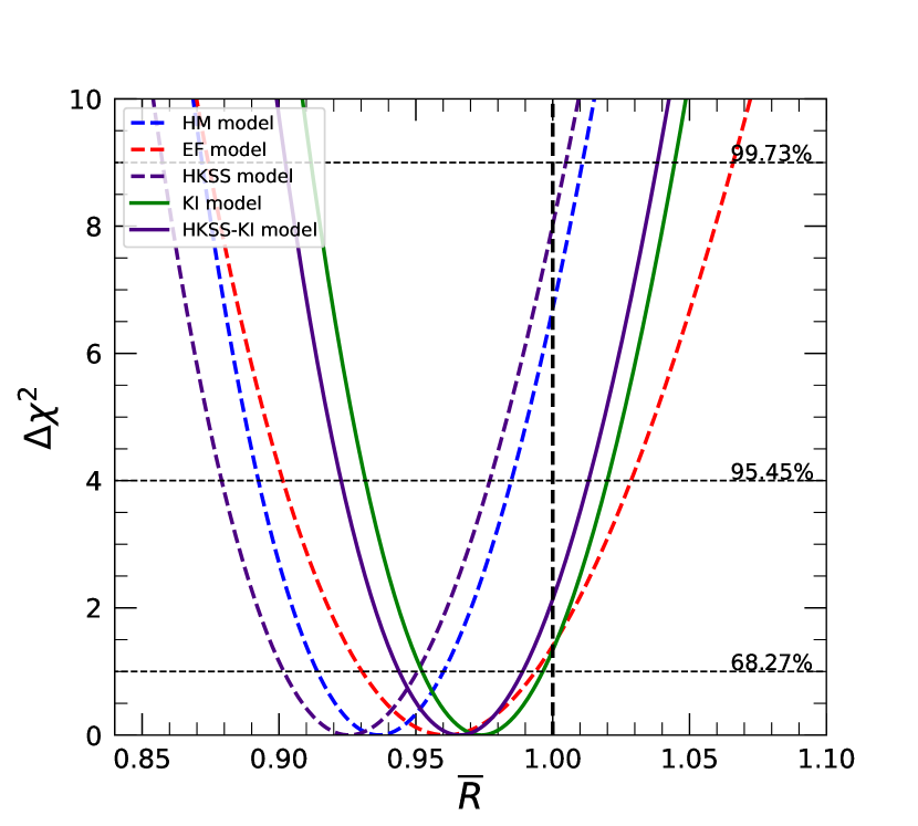
We performed the fit of the reactor rates considering a constant new physics suppression $R_{\text{NP}}^{a}=\overline{R}$ in the least-squares function (4). Figure 1 shows the value of $\Delta\chi^{2}=\chi^{2}-\chi^{2}_{\text{min}}$ as a function of the average ratio $\overline{R}$ obtained in our least-squares analysis for the five models listed in Section II, considering the IBD yields given in Table 3. The best-fit value of $\overline{R}$ for each of the five models and the corresponding statistical significance of the reactor antineutrino anomaly are given in Table 5.

Figure 2: Ratio $R_{a,\text{HM}}^{\text{exp}}$ of measured and expected IBD yields for the reactor experiments considered in our analysis as a function of the reactor-detector distance $L$ for the HM model. The error bars show the experimental uncertainties. The horizontal green band shows the average ratio $\overline{R}_{\text{HM}}$ and its uncertainty, that gives a $2.5\,\sigma$ RAA.

(a)  EF model [18]: no RAA ($1.2\,\sigma$).

(b)  HKSS model [22]: RAA ($2.9\,\sigma$).

(c)  KI model [24]: no RAA ($1.1\,\sigma$).

(d)  HKSS-KI model: no RAA ($1.5\,\sigma$).

Figure 3: Ratio of measured and expected IBD yields for the reactor experiments considered in our analysis as a function of the reactor-detector distance $L$ for the EF, HKSS, KI, and HKSS-KI models. The error bars show the experimental uncertainties. The horizontal green bands show the average ratio $\overline{R}$ and its uncertainty that we obtained for each model.

Figure 4: Red: results of the linear fits of 4+4 the Daya Bay [25] evolution data and 4+4 the RENO [27] evolution data. Blue: the corresponding predictions of the five models in Table 3.

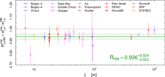
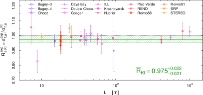
Let us discuss first our results for the HM model, that can be considered as the benchmark model, since it is the original model that gave rise to the reactor antineutrino anomaly. Figure 2 shows the ratios of measured and expected rates for the reactor experiments considered in our analysis and the result for the average ratio $\overline{R}_{\text{HM}}$ obtained with the HM model: $\overline{R}_{\text{HM}}=0.936{}^{+0.024}_{-0.023}$. This value of $\overline{R}_{\text{HM}}$ shows that the HM model implies a reactor antineutrino anomaly with a statistical significance of about $2.5\,\sigma$.

The statistical significance of the HM RAA that we have obtained is similar to that obtained using the original HM IBD yields in Table 3, which give $\overline{R}_{\text{HM}}^{\text{orig}}=0.943{}^{+0.021}_{-0.020}$, corresponding to a $2.6\,\sigma$ RAA.

The $2.5\,\sigma$ that we have obtained for the statistical significance of the HM RAA is smaller than that obtained using the least-squares function constructed with the method (A) described in Section III, which gives $\overline{R}_{\text{HM}}^{\text{(A)}}=0.922\pm 0.024$, corresponding to a $3.3\,\sigma$ RAA. The smallness of $\overline{R}_{\text{HM}}^{\text{(A)}}$ is a manifestation of the PPP problem discussed in Section III: the average ratio is smaller than most of the experimental ratios and generates a misleading larger value of the statistical significance of the HM RAA.

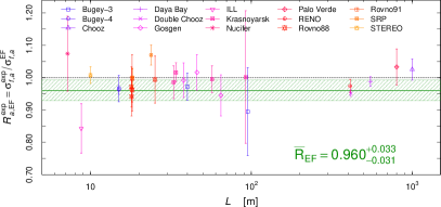
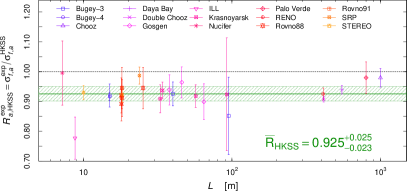
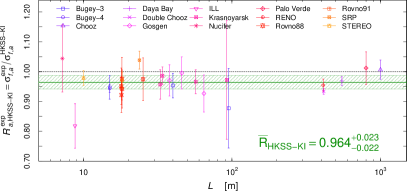
Let us now consider the four new models EF, HKSS, KI, and HKSS-KI discussed in Section II. The four panels in Figure 3 show the ratios of measured and expected rates for the reactor experiments considered in our analysis and the result for the average ratio in each model.

Figure 3(a) shows that with the EF calculation of the reactor antineutrino fluxes there is practically no RAA, since $\overline{R}_{\text{EF}}$ differs from unity by only $1.2\,\sigma$. This difference is almost equal to that given by the original EF IBD yields in Table 3. Note that using the least-squares function constructed with the method (A) described in Section III one would get a very misleading result: $\overline{R}_{\text{EF}}^{\text{(A)}}=0.911\pm 0.023$, corresponding to a spurious indication of a $3.9\,\sigma$ RAA. This strong effect of PPP is due to the large uncertainties of the EF fluxes that generate a strongly correlated covariance matrix when they are added in quadrature to the experimental uncertainties according to the prescription of method (A).

On the other hand, Figure 3(b) shows that with the HKSS model we obtain $\overline{R}_{\text{HKSS}}=0.925{}^{+0.025}_{-0.023}$, corresponding to a $2.9\,\sigma$ RAA, that is larger than the $2.5\,\sigma$ RAA obtained with the HM model. Also in this case the method (A) gives an unbalanced average value $\overline{R}_{\text{HKSS}}^{\text{(A)}}=0.910\pm 0.024$, corresponding to an excessive $3.7\,\sigma$ RAA.

Figure 3(c) shows that the reduced KI ${}^{235}\text{U}$ IBD yield leads to the practical disappearance of the RAA, since $\overline{R}_{\text{KI}}$ differs from unity by only $1.1\,\sigma$. From Figure 3(d) one can see that the addition of the HKSS corrections due to forbidden $\beta$ decays slightly increases the RAA to $1.5\,\sigma$. Also for these two models the estimation of the RAA would be misleading by adopting the least-squares method (A), that gives the unbalanced ratios $\overline{R}_{\text{KI}}^{\text{(A)}}=0.962\pm 0.022$ ($1.8\,\sigma$) and $\overline{R}_{\text{HKSS-KI}}^{\text{(A)}}=0.950\pm 0.022$ ($2.2\,\sigma$).

Summarizing the results of this Section, we have shown in a quantitative way that the HM and HKSS conversion models of the reactor antineutrino fluxes give a reactor antineutrino anomaly that is, however, not very large: $2.5\,\sigma$ and $2.9\,\sigma$, respectively. On the other hand, we do not have a significant anomaly if we assume the EF reactor antineutrino fluxes obtained from the nuclear databases with the summation method. Also the KI reduction of the ${}^{235}\text{U}$ IBD yield obtained with the conversion method leads to the practical disappearance of the reactor antineutrino anomaly, especially without the HKSS corrections. Therefore, there is an approximate agreement between the results of the summation method implemented in the EF model and the conversion method with the KI reduction of the ${}^{235}\text{U}$ IBD yield. There is, however, some concern regarding the problem of the 5 MeV bump, that is not fitted by the EF summation spectra and the KI conversion spectra. Since the HKSS corrections give only a partial explanation of the 5 MeV bump, the problem of the calculation of the reactor antineutrino fluxes needs further studies. We also think that the KI reduction of the ${}^{235}\text{U}$ IBD yield should be checked at least by an independent experiment.

V Fit of reactor fuel evolution data

The Daya Bay [25] and RENO [27] collaborations have published measurements of the IBD yield during the evolution of the reactor fuel in multiple cycles. These data provide important information on the reactor fluxes and can constrain reactor flux models and new physics [32, 33, 34, 35, 36, 37].

To compare the flux evolution data with the different model predictions, we first fit the evolution data with a linear function describing the IBD yield as a function of $f_{239}$, as done by the Daya Bay [25] and RENO [27] collaborations:

$$\sigma_{f,a}^{\text{lin}}=\bar{\sigma}_{f}+\dfrac{d\sigma_{f}}{df_{239}}\left(f_{239}^{a}-\bar{f}_{239}\right),$$ (6)

where $\overline{\sigma}_{f}$ is the average IBD yield and $d\sigma_{f}/df_{239}$ is the change in the IBD yield per unit change in the ${}^{239}\text{Pu}$ fission fraction. The linear approximation is justified by the approximately linear variations of the ${}^{235}\text{U}$, ${}^{238}\text{U}$, and ${}^{241}\text{Pu}$ fission fractions as function of the ${}^{239}\text{Pu}$ fission fraction in Daya Bay (see Figure 1 of Ref. [25]) and RENO (see Figure 1 of Ref. [27]). The model predictions for the average IBD yields and $d\sigma_{f}/df_{239}$ are obtained from the uncertainty propagation taking into account the experimental fission fraction variations and theoretical model correlations.

We performed the linear analysis of the Daya Bay and RENO evolution data with the least-squares function

$$\chi^{2}_{\text{lin}}=\sum_{a,b}\left(\sigma_{f,a}^{\text{exp}}-\sigma_{f,a}^{\text{lin}}\right)\left(V^{\rm exp}\right)_{ab}^{-1}\left(\sigma_{f,b}^{\text{exp}}-\sigma_{f,b}^{\text{lin}}\right),$$ (7)

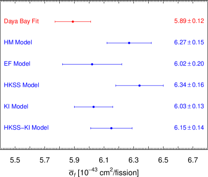
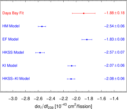
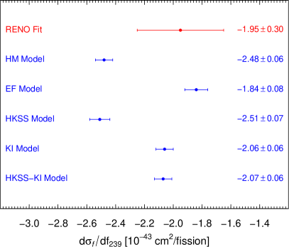
where $V^{\rm exp}$ is the experimental covariance matrix with statistical and systematic uncertainties added in quadrature. The results are shown in Figure 4, in comparison with the predictions of the five models in Table 3.

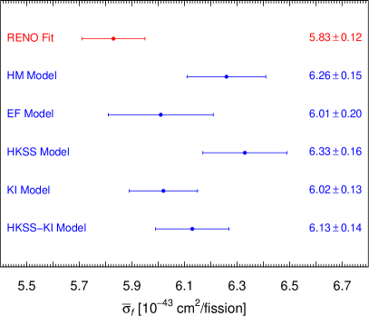
One can see from Figure 4 that the HM and HKSS models give values of $\bar{\sigma}_{f}$ and $d\sigma_{f}/df_{239}$ that are in tension with the linear fits of the evolution data. The discrepancies in $\bar{\sigma}_{f}$ are equivalent to the average suppressions of the Daya Bay and RENO IBD yields in the reactor antineutrino anomaly. The discrepancy of $d\sigma_{f}/df_{239}$ is an additional information that tells us that there are different suppressions of the ${}^{235}\text{U}$, ${}^{238}\text{U}$, ${}^{239}\text{Pu}$ and ${}^{241}\text{Pu}$ fluxes with respect to those predicted by the HM and HKSS models. The determination of the different suppressions has been discussed in several papers [25, 32, 33, 34, 35, 27, 36, 37]. Here we note that the $d\sigma_{f}/df_{239}$ tension for the HM and HKSS models is especially strong for the Daya Bay evolution data, as shown in Figure 4: $3.5\,\sigma$ for the HM model and $3.6\,\sigma$ for the HKSS model. Therefore, the HM and HKSS models are disfavored by the evolution data.

On the other hand, Figure 4 shows that the EF, KI and HKSS-KI models give values of $\bar{\sigma}_{f}$ and $d\sigma_{f}/df_{239}$ that agree with the fit of the evolution data within the uncertainties. Therefore these models are preferred by the evolution data not only for the absence of the reactor antineutrino anomaly, but also for a better fit of the slope $d\sigma_{f}/df_{239}$.

It is also interesting to fit the evolution data with the least-squares function in Eq. (4) and a constant new physics suppression $R_{\text{NP}}^{a}=\overline{R}$ as we have done in Section IV for the reactor rates. Table 5 shows the results for the five models under consideration, by comparing the values of the fits of the reactor rates, the evolution data and the combined rates and evolution data. The combined fit is done by considering the Daya Bay and RENO evolution data instead of the corresponding rates in Table II. One can see that the inclusion in the analysis of the evolution data confirms the existence of a reactor antineutrino anomaly for the HM ($2.8\,\sigma$) and HKSS ($3.0\,\sigma$) models and the absence of the anomaly for the EF model (only $0.8\,\sigma$). This is due to the good fit of the evolution data by the EF model, that has the smallest ${}^{235}\text{U}$ IBD yield, with a ratio of about 0.940 with respect to that in the original HM model in Table 3. This ratio is close to the best-fit ratio of $0.925\pm 0.015$ [36], obtained assuming the HM model for the other IBD yields, which, however, are not very different in the EF and original HM model (in the EF model, for the other important ${}^{239}\text{Pu}$ IBD yield there is only the very small increase of 0.5% with respect to the original HM model).

The KI and HKSS-KI models do not fit the evolution data as well as the EF model, because they have larger ${}^{235}\text{U}$ IBD yields and similar ${}^{239}\text{Pu}$ IBD yields. Therefore, the inclusion in the analysis of the evolution data increases the differences of $\overline{R}_{\text{KI}}$ and $\overline{R}_{\text{HKSS-KI}}$ from unity. However, the resulting $1.4\,\sigma$ for the KI model and $1.8\,\sigma$ for the HKSS-KI model are still too small to claim an anomaly.

VI Best-fit reactor flux model

It is useful to establish which of the five models in Table 3 provides the best fit of the reactor rates and the evolution data. We have already seen in Sections IV and V that the predictions of the HM and HKSS models are in tension with the reactor rates and with the Daya Bay and RENO evolution data. The EF models appears to be favorite as the best-fit model, with a difference of $\overline{R}_{\text{EF}}$ from unity of only $0.8\,\sigma$ considering the reactor rates and evolution data. Among the conversion models the KI model seems to be favorite, with a difference of $\overline{R}_{\text{KI}}$ from unity of $1.4\,\sigma$, and the addition of the HKSS corrections are disfavored by the $1.8\,\sigma$ difference of $\overline{R}_{\text{HKSS-KI}}$ from unity. In this section we apply goodness of fit tests to the reactor rates and evolution data with the aims to check these indications and to select the best-fit model.

If the fluctuations of the data with respect to the model prediction are Gaussian, the probability distribution function is given by

$$p(\sigma_{f,1}^{\text{exp}},\ldots,\sigma_{f,N}^{\text{exp}})=\dfrac{e^{-\chi^{2}_{\text{tot}}/2}}{\sqrt{(2\pi)^{N}|V^{\text{tot}}|}},$$ (8)

with

$$\chi^{2}_{\text{tot}}=\sum_{a,b}\left(\sigma_{f,a}^{\text{exp}}-\sigma_{f,a}^{\text{mod}}\right)\left(V^{\text{tot}}\right)^{-1}_{ab}\left(\sigma_{f,b}^{\text{exp}}-\sigma_{f,b}^{\text{mod}}\right),$$ (9)

where $N$ is the number of data points and $V^{\text{tot}}$ is the total covariance matrix with experimental and theoretical uncertainties added in quadrature. Note that Eq. (9) considered as a least-squares function would correspond to method (A) discussed in Section III, which suffers of the PPP problem in the determination of the average suppression of the data with respect to the model predictions. Since here we discuss the goodness of fit of the data for fixed model predictions, there is no PPP problem and it is appropriate to consider the Gaussian probability distribution function in Eqs. (8) and (9).

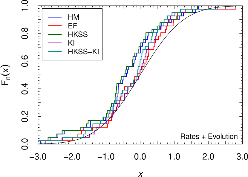
Table 6 shows that the standard $\chi^{2}$ goodness of fit test is not able to reject any of the five models under consideration if we consider the usual minimum $p$-value of 5% corresponding to a confidence level of 95%. However, if the distribution of the data is Gaussian, there should be an approximately equal number of positive and negative deviations of the data from the model predictions. This characteristic is not taken into account by the standard $\chi^{2}$ goodness of fit test, that is not sensitive to the signs of the deviations of the data with respect to the model predictions. From Figures 2 and 3(b) one can see that most of the reactor rates are smaller than the corresponding predictions of the HM and HKSS models (corresponding to $R_{a,\text{mod}}^{\text{exp}}=1$), whereas Figures 3(a), 3(c), and 3(d) show that the signs of the fluctuations of the reactor rates are more balanced for the EF, KI, and HKSS-KI models, especially for the EF model. Therefore statistical tests that are sensitive to the signs of the deviations should disfavor the HM and HKSS models with respect to the EF, KI, and HKSS-KI models and hopefully indicate which of these models provides the best fit of the data.

In order to perform statistical tests that probe the Gaussian distribution of the data taking into account the signs of the deviations from the model predictions, we need to transform the data to a univariate normal distribution. This is achieved by considering the transformed data

$$x_{a}^{\text{mod}}=\sum_{b}\left(V^{\text{tot}}\right)^{-1/2}_{ab}\left(\sigma_{f,b}^{\text{exp}}-\sigma_{f,b}^{\text{mod}}\right),$$ (10)

that should have a Gaussian distribution with zero mean and unit standard deviation.

We first checked with the Shapiro-Wilk test (SW) that the transformed data $x_{a}^{\text{mod}}$ have an empirical Gaussian distribution around the sample mean. Table 6 shows that the transformed data pass this test with a $p$-value larger than 5% for all the models under consideration, except the reactor rates for the EF model, that have a $p$-value of $4\%$. This is somewhat puzzling, because the other tests discussed below confirm the expectation that the EF model is currently the best one.

We applied the following statistical tests that are sensitive to the sign and size of the deviations of the transformed data with respect to the Gaussian distribution with zero mean and unit standard deviation:

Test	HM	EF	HKSS	KI	HKSS-KI
	Rates
$\bm{\chi^{2}}$	$0.21$	$0.08$	$0.12$	$0.43$	$0.21$
SW	$0.14$	$0.04$	$0.13$	$0.20$	$0.13$
sign	$0.01$	$0.50$	$<10^{-3}$	$0.22$	$0.12$
KS	$0.01$	$0.77$	$0.004$	$0.36$	$0.19$
CVM	$0.01$	$0.74$	$0.005$	$0.37$	$0.17$
AD	$0.02$	$0.50$	$0.006$	$0.39$	$0.17$
$\bm{Z_{\textbf{K}}}$	$<10^{-3}$	$0.004$	$<10^{-3}$	$0.06$	$0.01$
$\bm{Z_{\textbf{C}}}$	$0.01$	$0.02$	$0.005$	$0.41$	$0.06$
$\bm{Z_{\textbf{A}}}$	$0.02$	$0.13$	$0.009$	$0.38$	$0.12$
weighted average	$0.06$	$0.29$	$0.04$	$0.45$	$0.16$
	Evolution
$\bm{\chi^{2}}$	$0.08$	$0.86$	$0.05$	$0.86$	$0.71$
SW	$0.70$	$0.94$	$0.66$	$0.19$	$0.20$
sign	$0.11$	$0.23$	$0.04$	$0.40$	$0.11$
KS	$0.13$	$0.45$	$0.06$	$0.46$	$0.21$
CVM	$0.05$	$0.56$	$0.02$	$0.37$	$0.10$
AD	$0.03$	$0.64$	$0.01$	$0.36$	$0.09$
$\bm{Z_{\textbf{K}}}$	$<10^{-3}$	$0.02$	$<10^{-3}$	$0.003$	$<10^{-3}$
$\bm{Z_{\textbf{C}}}$	$0.03$	$0.54$	$0.01$	$0.19$	$0.08$
$\bm{Z_{\textbf{A}}}$	$0.05$	$0.63$	$0.02$	$0.16$	$0.05$
weighted average	$0.08$	$0.50$	$0.05$	$0.27$	$0.11$
	Rates + Evolution
$\bm{\chi^{2}}$	$0.13$	$0.22$	$0.08$	$0.68$	$0.44$
SW	$0.32$	$0.13$	$0.35$	$0.59$	$0.41$
sign	$0.03$	$0.38$	$0.006$	$0.38$	$0.11$
KS	$0.04$	$0.84$	$0.02$	$0.39$	$0.20$
CVM	$0.02$	$0.67$	$0.006$	$0.38$	$0.14$
AD	$0.02$	$0.57$	$0.006$	$0.40$	$0.13$
$\bm{Z_{\textbf{K}}}$	$<10^{-3}$	$0.05$	$<10^{-3}$	$0.05$	$0.008$
$\bm{Z_{\textbf{C}}}$	$0.02$	$0.11$	$0.005$	$0.55$	$0.15$
$\bm{Z_{\textbf{A}}}$	$0.03$	$0.20$	$0.01$	$0.41$	$0.12$
weighted average	$0.05$	$0.35$	$0.03$	$0.42$	$0.16$

Table 6: $p$-values of goodness of fit tests of the reactor rates in Table II and of the Daya Bay [25] and RENO [27] evolution data for the five models in Table 3. The tests are: $\chi^{2}$, Shapiro-Wilk (SW), sign test (sign), Kolmogorov-Smirnov test (KS), Cramer-von Mises test (CVM), Anderson-Darling test (AD), and the $Z_{\text{K}}$, $Z_{\text{C}}$, and $Z_{\text{A}}$ tests [62]. The weighted averages are calculated by averaging for each model the $p$-values of the different tests normalized to unity.

(a) Reactor rates.

(b) Daya Bay and RENO evolution.

(c) Rates + evolution.

Figure 5: Empirical cumulative distribution functions of 5(a) the reactor rates in Table II, 5(b) the Daya Bay [25] and RENO [27] evolution data, and 5(c) the rates and evolution data, assuming Gaussian distributions with respect to the predictions of the five models in Table 3. The black curves shows the cumulative distribution function of the Gaussian distribution with zero mean and unit standard deviation.

Sign test

This classical test depends on the quantities of positive and negative deviations of the transformed data with respect to the Gaussian distribution with zero mean and unit standard deviation, that should be approximately equal. Table 6 shows that the sign test excludes the HM and HKSS models, that have $p$-values smaller than 5% for the reactor rates and in the combined analysis of the rates and evolution data. The HKSS model has also a $p$-value smaller than 5% in the analysis of the evolution data alone. The other models perform well under this test, with the EF model preferred by the reactor rates, the KI model preferred by the evolution data and equal $p$-values for the two models in the combined analysis of the rates and evolution data.

Kolmogorov-Smirnov test (KS)

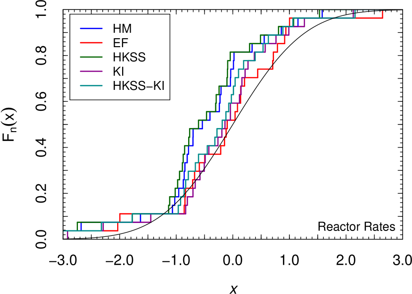
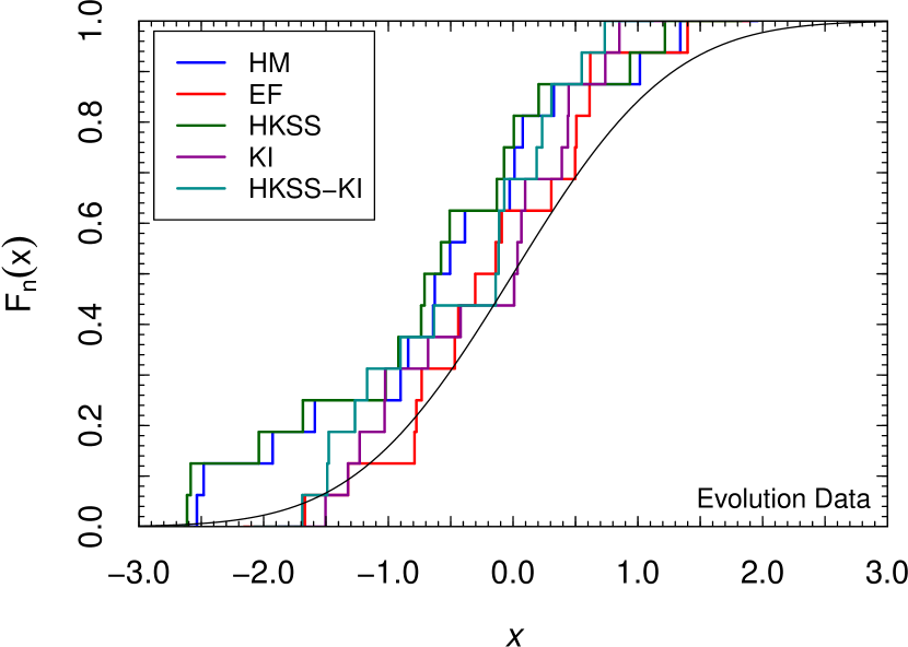
This classical test depends on the maximum distance between the empirical cumulative distribution function of the sample and the theoretical cumulative distribution function (see Figure 5). Since the KS test does not probe the whole differences of the two cumulative distribution functions it is not very powerful. However, as one can see from Table 6, the KS test disfavors the HM and HKSS model, that have $p$-values smaller than 5% for the reactor rates and in the combined analysis of the rates and evolution data. The reactor rates and the combined analysis of the rates and evolution data favor the EF model. However, the EF and KI models have practically equal $p$-values in the analysis of the the evolution data alone.

Cramer-von Mises test (CVM)

This classical test depends on the integral difference between the empirical cumulative distribution function of the sample and the theoretical cumulative distribution function (see Figure 5). Table 6 shows that, considering $p$-values smaller than 5%, the CVM test disfavors the HM and HKSS models in the analysis of the reactor rates and in the combined analysis of the rates and evolution data. The evolution data alone disfavor the HKSS model, with the HM model having the borderline $p$-value of 5%. The other models pass the test, but the EF model is favorite by all the three data analyses.

Anderson-Darling test (AD)

Also this classical test depends on the integral difference between the empirical cumulative distribution function of the sample and the theoretical cumulative distribution function (see Figure 5). It differs from the CVM test by placing more weight on observations in the tails of the distribution. As one can see from Table 6, this test disfavors the HM and HKSS models, that have $p$-values smaller than 5%, and favor the EF model in all the three data analyses.

$Z_{\text{K}}$, $Z_{\text{C}}$, and $Z_{\text{A}}$ tests

These tests [62] are relatively new tests that are similar, respectively, to the classical KS, CVM, and AD tests, with more powerful measures, based on the likelihood ratio, of the difference between the empirical cumulative distribution function of the sample and the theoretical cumulative distribution function. One can see from Table 6 that in particular the $Z_{\text{K}}$ test is very powerful for rejecting the HM and HKSS models, that have $p$-values smaller than 0.1% in all the three data analyses. The $Z_{\text{K}}$ test disfavors also the HKSS-KI model, with a $p$-value of 0.1% for the reactor rates and smaller $p$-value for the other two data analyses. For the reactor rates, the three tests favor the KI model, with the EF model performing very badly in the $Z_{\text{K}}$ test ($0.4\%$ $p$-value) and badly in the $Z_{\text{C}}$ test ($2\%$ $p$-value). On the other hand, for the evolution data the three tests prefer the EF model, although it has a $Z_{\text{K}}$ $p$-value of only $2\%$. The $Z_{\text{K}}$ $p$-value of the KI model is worse: $0.3\%$. Both the EF and KI models are accepted by the three tests in the combined analysis of the rates and evolution data, with a preference for the KI model in the $Z_{\text{C}}$ and $Z_{\text{A}}$ tests.

Figure 6: Contours of the $2\sigma$ allowed regions in the ($\sin^{2}\!2\vartheta_{ee},\Delta{m}^{2}_{41}$) plane obtained from the neutrino oscillation fit of 6 the reactor rates in Table II and 6 the combined fit of the reactor rates and the Daya Bay [25] and RENO [27] evolution data. The blue, red, green, magenta, and cyan curves correspond, respectively, to the HM, EF, HKSS, KI, and HKSS-KI models in Table 3. Also shown are the contour of the $2\sigma$ allowed regions of the Gallium anomaly obtained in Ref. [63] from the combined analysis of the GALLEX, SAGE and BEST data (orange curve), and the $2\sigma$ bound obtained from the analysis of solar neutrino data in Ref. [64] (dark red vertical line).

Considering the overall performance of the five models under consideration under the goodness of fit tests that we have performed, we can conclude that the HM and HKSS models are excluded by the data with a high confidence level. Note that this conclusion is supported not only by the powerful relatively new $Z_{\text{K}}$ test, but also by the classical sign test and, especially for the HKSS model, by the classical KS, CVM and AD tests. The HM and HKSS models are rejected with these classical tests by the analysis of the reactor rates and the combined analysis of reactor rates and evolution data. The evolution data alone are less powerful in rejecting these models, because they are less numerous, they have a smaller variability of the fuel fractions, and they have large correlated systematic uncertainties.

We have seen that among the other models, the HKSS-KI model is not the best one for any test and it is strongly disfavored by the $Z_{\text{K}}$ test applied to the combined analysis of reactor rates and evolution data.

The EF and KI models are alternatively the best for some test in each of the three data analyses. In order to try to establish a ranking, we consider the weighted averages of the $p$-values of the tests for each of the three analyses in Table 6. These weighted averages have been obtained by averaging for each model the $p$-values of the different tests normalized to unity. Such normalization is necessary in order to weight equally the different tests, including those that give small $p$-values for all the models. Let us however emphasize that these weighted averages do not have a statistical meaning and are only helpful for establishing an indicative ranking of the models. From the values of the weighted averages reported in Table 6 one can see that the KI model is favored by the reactor rates and the EF model is favored by the evolution data. The combined analysis of reactor rates and evolution data slightly favors the KI model, with an average $p$-value of $42\%$, but the EF model has the almost as good average $p$-value of $35\%$.

In conclusion of this attempt to find the best-fit reactor flux model, since the EF and KI models are preferred by different tests and sets of data, with similar overall performances in the combined analysis of reactor rates and evolution data, it is fair to consider both as favorite, specifying that they have been obtained with different methods: the EF model has been obtained entirely with the summation method, and the KI model has been obtained entirely with the conversion method. The strongly disfavored HM and HKSS models can be considered in practice as conversion models, because only the minor ${}^{238}\text{U}$ neutrino flux has been calculated with the summation method. Since we obtained the HKSS-KI model by reducing the ${}^{235}\text{U}$ IBD yield of the HKSS model by the KI factor and keeping the same ${}^{238}\text{U}$, ${}^{239}\text{Pu}$, and ${}^{241}\text{Pu}$ neutrino fluxes of the HKSS model (see Section II), also the HKSS-KI model can be considered in practice as a conversion model. Therefore, from our analysis we conclude that the KI model is the best among the conversion models and the only summation model that we considered, the EF model, is practically equally good.

VII Neutrino oscillations

In this section we discuss the implications of the reactor neutrino flux models for the neutrino oscillation analysis of the short-baseline reactor neutrino data. We consider the effective 3+1 survival probability of electron neutrinos and antineutrinos in Eq. (1). However, since the reactor neutrino measurements can probe only the disappearance of electron antineutrinos the results apply to any model of neutrino masses and mixing that predicts an effective two-neutrino-like survival probability of the type in Eq. (1), that depends only on an effective mixing angle $\vartheta_{ee}$ and a squared-mass difference $\Delta m_{41}^{2}$.

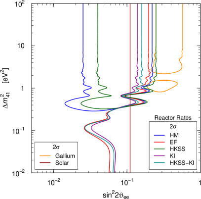
Figure 6 shows the contours of the $2\sigma$ allowed regions in the ($\sin^{2}\!2\vartheta_{ee},\Delta{m}^{2}_{41}$) plane obtained from the neutrino oscillation fit of the reactor rates in Table II considering the IBD yields of the HM, EF, HKSS, KI, and HKSS-KI models in Table 3. One can see that there is an indication in favor of neutrino oscillations only for the HM and HKSS models that give a significant reactor rate anomaly above $2\sigma$, as discussed in Section IV (see Table 5). Considering the EF, KI, and HKSS-KI models, for which the reactor rate anomaly is smaller than $2\sigma$, we obtained the $2\sigma$ exclusion curves shown in Figure 6, that allow only small values of $\sin^{2}2\vartheta_{ee}$, including $\sin^{2}2\vartheta_{ee}=0$, that corresponds to the absence of short-baseline oscillations.

For all the reactor flux models, there are upper bounds for the value of the mixing parameter $\sin^{2}2\vartheta_{ee}$ that depend on the value of $\Delta m_{41}^{2}$. For $\Delta m_{41}^{2}\gtrsim 2\,\text{eV}^{2}$ the upper bounds for $\sin^{2}2\vartheta_{ee}$ are between $0.14$ and $0.25$ for all the reactor flux models.

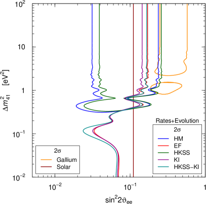
In Figure 6 we also reproduced the contours of the regions that are allowed at $2\sigma$ by the Gallium anomaly, according to the combined analysis in Ref. [63] of the new data of the BEST experiment and the old data of the GALLEX [65] and SAGE [66] experiments. One can see that the Gallium anomaly region lies at rather large values of $\sin^{2}2\vartheta_{ee}$ and is in tension with the reactor upper bounds on $\sin^{2}2\vartheta_{ee}$ for all the reactor flux models. The Gallium anomaly region is also in strong tension with the more stringent $2\sigma$ solar electron neutrino upper bound $\sin^{2}2\vartheta_{ee}<0.11$ [64] shown in Figure 6 (see Refs. [67, 68, 69, 70, 53, 71, 72] for previous analyses that constrained $\sin^{2}2\vartheta_{ee}$ using the solar electron neutrino data).

Figure 6 shows the contours of the $2\sigma$ allowed regions in the ($\sin^{2}\!2\vartheta_{ee},\Delta{m}^{2}_{41}$) plane obtained from the combined neutrino oscillation fit of the reactor rates and the Daya Bay [25] and RENO [27] evolution data. One can see that the allowed regions are similar to those obtained in Figure 6 without the evolution data. The reason is that the main information on neutrino oscillations coming from the Daya Bay and RENO evolution data is given by the comparison of the measured average rates with the model predictions, that is already taken into account in the rate analysis.

Considering the EF and KI models that are favored according to the discussion in Section VI assuming the absence of neutrino oscillations, the $2\sigma$ upper bounds on $\sin^{2}2\vartheta_{ee}$ for $\Delta m_{41}^{2}\gtrsim 2\,\text{eV}^{2}$ are, respectively, $0.20$ and $0.14$ from the rates analysis, and $0.17$ and $0.14$ from the combined rates and evolution analysis. Therefore, there is a significant tension with the $2\sigma$ allowed region of the Gallium anomaly, that lies above $\sin^{2}2\vartheta_{ee}\approx 0.2$.

The tension between the Gallium anomaly obtained in Ref. [63] and the exclusion curves of the DANSS [73], PROSPECT [74], and STEREO [75], experiments is shown in Figure 2 of Ref. [76], where one can see that, however, there is a partial compatibility for $\Delta m_{41}^{2}\approx 9\,\text{eV}^{2}$. The exclusion curves of these experiments are obtained comparing the reactor neutrino induced spectrum at different distances around 10 m. They disappear for $\Delta m_{41}^{2}\gtrsim 10\,\text{eV}^{2}$. Therefore, these experiments cannot probe the high-$\Delta m_{41}^{2}$ part of the Gallium anomaly region. The results of our analyses of the reactor rates and the reactor evolution data fills this gap and extends the tension between the reactor neutrino data and the Gallium anomaly to large values of $\Delta m_{41}^{2}$.

VIII Summary and conclusions

In this paper we revisited the reactor antineutrino anomaly in light of the recent reactor antineutrino flux calculations.

We have first performed, in Section II, an improved calculation of the IBD yields of five reactor antineutrino flux models: the HM [7, 8], HKSS [22], KI [24], and HKSS-KI conversion models and the EF [18] summation model. The HM model has been considered the standard one since 2011 and is the basis of the reactor antineutrino anomaly [9, 46]. The HKSS model was proposed in 2019 as an improvement of the HM model that gives a partial explanation of the 5 MeV bump obtained by taking into account forbidden $\beta$ decays. The KI model, proposed in 2021, is based on a decrease of the ${}^{235}\text{U}$ antineutrino flux obtained with the conversion method motivated by new relative measurements of the ratio of the ${}^{235}\text{U}$ and ${}^{239}\text{Pu}$ $\beta$ spectra at the Kurchatov Institute. The HKSS-KI model is a model that we obtained by applying to the HKSS model the KI suppression of the ${}^{235}\text{U}$ antineutrino flux. The EF model is the most updated summation model, that was published in 2019. The improved IBD yields that we obtained for the EF model agree very well with the original ones [18], whereas those of the HM, HKSS, and KI model are slightly larger than the original ones (see Tables 3 and 3).

Then, after a discussion in Section III of the proper statistical method for the analysis of the data, we calculated the suppression of the reactor antineutrino flux predicted by each of the 5 models that is necessary for fitting the rates measured by the experiments listed in Table II (Section IV). We found that, the reactor antineutrino anomaly is larger than $2\sigma$ only for the HM and HKSS models. The difference between the data and the predictions of the EF and KI models is slightly larger than $1\sigma$ (see Table 5). It slightly increases to $1.5\,\sigma$ for the HKSS-KI model. Therefore there is practically no anomaly for the EF, KI, and HKSS-KI models. The addition of the Daya Bay [25] and RENO [27] evolution data discussed in Section V confirms these conclusions, but establish a more pronounced ranking of the models, with the EF model having the smallest deviation from the data ($0.8\,\sigma$), followed by the KI model ($1.4\,\sigma$), and the HKSS-KI model ($1.8\,\sigma$).

In Section VI we further explored the question of which is the best-fit model by applying several goodness of fit tests. This is an important question, because although there is an approximate agreement of the new EF summation model and the new KI and HKSS-KI conversion models on the demise of the reactor antineutrino anomaly, the models are different and have different IBD yields (see Table 3). We found that the EF and KI models are favored, with the EF model fitting better the evolution data and the KI model fitting better the reactor rates. Therefore, we can consider EF as the best summation model and KI as the best conversion model, leaving the decision of a clear preference between the two models to future studies with more data.

We finally discussed the implications of the five models for short-baseline neutrino oscillations due to active-sterile neutrino mixing. We have shown that the five models imply upper bounds that are not very different for the mixing generating the oscillations. Hence, this is a robust constraint given by reactor antineutrino data.

The reactor bound on active-sterile neutrino mixing agrees with the solar bound [64] and both bounds are in tension with the large mixing [63] required to explain the anomaly of the GALLEX [65], SAGE [66], and BEST [63] Gallium experiments with short baseline neutrino oscillations. This is a puzzling new development in the phenomenology of short-baseline neutrino oscillations that may require an explanation that goes beyond the simplest model of active-sterile neutrino mixing.