Applying quantum approximate optimization to
the heterogeneous vehicle routing problem

Abstract

Quantum computing offers new heuristics for combinatorial problems. With small- and intermediate-scale quantum devices becoming available, it is possible to implement and test these heuristics on small-size problems. A candidate for such combinatorial problems is the heterogeneous vehicle routing problem (HVRP): the problem of finding the optimal set of routes, given a heterogeneous fleet of vehicles with varying loading capacities, to deliver goods to a given set of customers. In this work, we investigate the potential use of a quantum computer to find approximate solutions to the HVRP using the quantum approximate optimization algorithm (QAOA). For this purpose we formulate a mapping of the HVRP to an Ising Hamiltonian and simulate the algorithm on problem instances of up to 21 qubits. We find that the number of qubits needed for this mapping scales quadratically with the number of customers. We compare the performance of different classical optimizers in the QAOA for varying problem size of the HVRP, finding a trade-off between optimizer performance and runtime.

I Introduction

Devices utilizing quantum-mechanical effects provide a new computational paradigm that enables novel algorithms and heuristics Shor (2002); Harrow et al. (2009); Montanaro (2016); Wendin (2017); Bharti et al. (2021). The ongoing development of such devices Arute et al. (2019); Bruzewicz et al. (2019); Kjaergaard et al. (2020); Zhong et al. (2020) provides an opportunity to test these algorithms on small problem instances, which could lead to new solutions to hard optimization problems. In this work, we show how a quantum approximate optimization algorithm (QAOA) Farhi et al. (2014) can be employed to find approximate solutions for the heterogeneous vehicle routing problem (HVRP) Koç et al. (2016). Our approach can be utilized on both noisy intermediate-scale quantum (NISQ) Preskill (2018) computers and quantum annealers Hauke et al. (2020). It also paves the way for implementing challenging instances of the HVRP on larger quantum computers in the future.

The HVRP belongs to the well known and extensively studied class of optimization problems known as the vehicle routing problem (VRP) Golden et al. (2008) in the field of logistics. The VRP captures the problem of finding the optimal set of routes for a fleet of vehicles to travel in order to deliver goods to a given set of customers. This problem is also found in supply-chain management and scheduling Caunhye et al. (2012). Variants of the VRP include the capacitated vehicle routing problem (CVRP), in which the vehicles have a limited carrying capacity Golden et al. (2008), and the HVRP studied here, in which the fleet composition is unknown and capacity constraints are given Koç et al. (2016); Ghandriz et al. (2021). All these VRPs are very challenging since they belong to the complexity class NP-hard Lenstra and Kan (1981).

Due to its industrial relevance, there has been tremendous effort devoted to finding good approximate solutions to the VRP and its variants through various heuristics Laporte et al. (2014); Tavares et al. (2009), e.g., construction heuristics Hwang et al. (1999), improvement heuristics Van Breedam (1995), and metaheuristic top-level strategies Brandstätter and Reimann (2018). In construction heuristics, e.g., the Clarke and Wright saving algorithm Clarke and Wright (1964), one starts from an empty solution and iteratively extends it until a complete solution is obtained. In improvement heuristics, one instead starts from a complete solution (often generated by a construction heuristic) and then try to improve further through local moves. There are several software libraries and tools that implement ready-to-use solvers for all these methods Lougee (2003); Groër et al. (2010); Perron and Furnon . Moreover, exact methods for solving the VRP and its variants have also been investigated Baldacci and Mingozzi (2009).

In this article, we instead investigate a heuristic method for solving the HVRP on a quantum computer. Such devices, including both programmable quantum processors Wendin (2017); Jazaeri et al. (2019); Kjaergaard et al. (2020) and quantum annealers Hauke et al. (2020), are gradually becoming available due to the recent advances in controlling quantum systems. The current quantum computers are known as NISQ devices Preskill (2018), since they are largely limited by their intermediate number (several tens Arute et al. (2019); Pino et al. (2021); Mooney et al. (2021); Blinov et al. (2021); Pogorelov et al. (2021); Wu et al. (2021)) of controllable qubits, limited connectivity, imperfect qubit control, short coherence times, and minimal error correction. Only a subset of known quantum algorithms can run on these near-term devices Kandala et al. (2017); Bharti et al. (2021); other algorithms require more advanced hardware.

The heuristic method we apply to the HVRP here is an example of a variational quantum algorithm (VQA) Cerezo et al. (2020), which is a promising class of quantum algorithms that are compatible with NISQ devices. These algorithms generally need access to a description of the problem, and also possibly to a set of training data. With this in hand, the first step is to define a cost (or loss) function $C$, which encodes the solution to the problem. Next, one proposes an ansatz, i.e., a quantum operation depending on a set of continuous or discrete parameters $\boldsymbol{\theta}$ that can be optimized. This ansatz is then optimized in a hybrid quantum-classical loop to solve the optimization task

$$\boldsymbol{\theta^{*}}=\underset{\boldsymbol{\theta}}{\text{argmin }}C(\boldsymbol{\theta}).$$ (1)

Such algorithms have emerged as a leading contender for obtaining quantum advantage Cerezo et al. (2020) within the constraints of NISQ devices. By now, variational quantum algorithms (VQAs) have been proposed for numerous applications that researchers have envisioned for quantum computers, e.g., in chemistry, logistics, and finance Stamatopoulos et al. (2020); Vikstål et al. (2020); Braine et al. (2021); Choi et al. (2019); Egger et al. (2021).

The type of VQA we employ here is the QAOA Farhi et al. (2014), which is a heuristic that can approximate the solution to many combinatorial problems, including VRPs. Current research in this area ranges from applications on large-scale VRP instances with a quantum annealer Syrichas and Crispin (2017) to more specific variants of the VRP, such as the CVRP Feld et al. (2019) or the multi-depot capacitated VRP Harikrishnakumar et al. (2020). These approximation algorithms have been tested on quantum annealers Feld et al. (2019) and NISQ devices Utkarsh et al. (2020). There have also been several experimental realizations of the QAOA applied to other optimization problems Harrigan et al. (2021); Bengtsson et al. (2020); Abrams et al. (2020); Willsch et al. (2020); Otterbach et al. (2017).

However, a problem description suited for the QAOA, an Ising Hamiltonian Ising (1925); Brush (1967); Lucas (2014) (describing the energy of interacting two-level systems), seems to be lacking for the case of the HVRP. In this work, we provide such a mapping for the HVRP, which can be utilized on both NISQ computers and quantum annealers. We show that, in this formulation, the number of qubits scales quadratically with the number of customers. To explore the performance of the QAOA applied to the HVRP, we simulate problem instances with up to 21 qubits. We check how this performance depends both on the choice of classical optimizer and on the depth of the quantum circuit. This work lays the foundation for finding approximate solutions to large problem instances of the HVRP when sufficiently advanced quantum-computing hardware becomes available.

The paper is organized as follows. In Sec. II, we introduce the HVRP and its mathematical formulation. Then, in Sec. III, we develop the Ising formulation of the HVRP. In Sec. IV, we review the QAOA and describe how it can be used to find approximate solutions to the HVRP. In Sec. V, we present numerical results from applying the QAOA to a few HVRPs of different sizes. Finally, we conclude the paper and give an outlook for future work in Sec. VI.

II The heterogeneous vehicle routing problem

The HVRP can be formulated as follows Koç et al. (2016). A fleet of vehicles is available at a depot, which becomes node 0 of a complete graph $\mathcal{G}=(\mathcal{N},\mathcal{E})$ (we do not consider multiple depots). Here, $\mathcal{N}=\{0,...,n\}$ is the set of nodes or vertices, such that the $n$ customers that the fleet of vehicles should deliver goods to constitute the customer set $\mathcal{N}_{0}=\mathcal{N}\setminus\{0\}$, and $\mathcal{E}=\{(i,j):0\leq i,j\leq n,i\neq j\}$ denotes the set of edges or arcs. Each customer $i$ has a positive demand $q_{i}$.

The set of available vehicle types is $\mathcal{V}=\{1,...,k\}$, with $m_{v}$ vehicles of type $v\in\mathcal{V}$. When using these vehicles to deliver goods to meet the customer demand, there are several costs and constraints that need to be taken into account. First, there is the fixed vehicle cost $t^{v}$, i.e., the cost that is independent of the distance travelled by the vehicle of type $v$. Then, there is the vehicle capacity $Q^{v}$. Note that different vehicle types can have the same capacities, but differ in, e.g., the type of powertrain used Ghandriz et al. (2021). Finally, there is the cost $c_{ij}^{v}$ of travelling on edge $(i,j)$ with the vehicle of type $v$. To describe all constraints, it is also useful to introduce the binary variables $x^{v}_{ij}$, which are equal to 1 if and only if a vehicle of type $v$ travels on edge $(i,j)$. Furthermore, we denote by $f_{ij}^{v}$ the amount of goods that are leaving node $i$ to go to node $j$ using truck $v$, while the amount of goods entering the node is denoted $f_{ji}^{v}$.

Using this notation, the HVRP is to minimize the cost

$$C_{\rm tot}=\sum_{v\in\mathcal{V}}\sum_{j\in\mathcal{N}_{0}}t^{v}x^{v}_{0j}+\sum_{v\in\mathcal{V}}\sum_{(i,j)\in\mathcal{E}}c^{v}_{ij}x^{v}_{ij}\,,$$ (2)

subject to the constraints

$$\sum_{j\in\mathcal{N}_{0}}x^{v}_{0j}\leq m_{v}\quad v\in\mathcal{V}\,,$$ (3)

$$\sum_{v\in\mathcal{V}}\sum_{j\in\mathcal{N}}x^{v}_{ij}=1\quad i\in\mathcal{N}_{0}\,,$$ (4)

$$\sum_{v\in\mathcal{V}}\sum_{i\in\mathcal{N}}x^{v}_{ij}=1\quad j\in\mathcal{N}_{0}\,,$$ (5)

$$\sum_{j\in\mathcal{N}_{0}}x^{v}_{j0}=\sum_{j\in\mathcal{N}_{0}}x^{v}_{0j}\quad v\in\mathcal{V}\,,$$ (6)

$$\sum_{v\in\mathcal{V}}\sum_{j\in\mathcal{N}}f^{v}_{ji}-\sum_{v\in\mathcal{V}}\sum_{j\in\mathcal{N}}f^{v}_{ij}=q_{i}\quad i\in\mathcal{N}_{0}\,,$$ (7)

$$q_{j}x_{ij}^{v}\leq f^{v}_{ij}\leq(Q_{v}-q_{i})x_{ij}^{v}\quad(i,j)\in\mathcal{E},v\in\mathcal{V}\,,$$ (8)

$$x_{ij}^{v}\in\{0,1\}\quad(i,j)\in\mathcal{E},v\in\mathcal{V}\,,$$ (9)

$$f^{v}_{ij}\geq 0\quad(i,j)\in\mathcal{E},v\in\mathcal{V}\,.$$ (10)

The objective function in Eq. (2) is the sum of the fixed vehicle cost for the vehicles used to deliver goods and the total (variable) travel cost for those vehicles. The constraint in Eq. (3) ensures that the maximum number of available vehicles for a specific vehicle type is not exceeded. The constraints in Eqs. (4) and (5) make sure that each customer is visited exactly once, and the constraint in Eq. (6) sees to that all vehicles leaving the depot return to it after delivering their goods. The constraints in Eqs. (7) and (8) ensure a correct commodity flow that meets all customer demands. Finally, the constraints in Eqs. (9) and (10) enforce the binary form and non-negativity restrictions on the variables.

III Ising formulation for the HVRP

All optimization problems in the complexity class NP can be reformulated as the problem of finding the ground state (lowest-energy configuration) of a quantum Hamiltonian Lucas (2014). This is also the method we use for the HVRP in this work. Since the HVRP combines two distinct problems, a routing problem and a capacity problem, we have to derive an Ising Hamiltonian that captures both these problems simultaneously.

III.1 Routing problem

For the routing problem, we start from the travelling salesperson problem (TSP) formulation given in Ref. Lucas (2014) with the Hamiltonian $H$ encoding the total cost:

$$H =H_{A}+H_{B}\,,$$ (11)

$$H_{A} =A\sum_{i=1}^{N}\left(1-\sum_{\alpha=1}^{N}y_{i\alpha}\right)^{2}+A\sum_{\alpha=1}^{N}\left(1-\sum_{i=1}^{N}y_{i\alpha}\right)^{2}$$

$$+A\sum_{(i,j)\notin\mathcal{E}}\sum_{\alpha=1}^{N}y_{i\alpha}y_{j\alpha+1}\,,$$ (12)

$$H_{B} =B\sum_{(i,j)\in\mathcal{E}}W_{ij}\sum_{\alpha=1}^{N}y_{i\alpha}y_{j\alpha+1}\,,$$ (13)

where $N=|\mathcal{N}|$ is the number of nodes including the depot, $A$ and $B$ are positive constants, and $W$ encodes the distances between the nodes. The index $i$ represents the nodes and $\alpha$ the order in a prospective cycle. The binary variables $y_{i\alpha}$ can be referred to as ’routing variables’ indicating in which order of the cycle node $i$ is visited. There are $N^{2}$ variables, with $y_{i,N+1}\equiv y_{i,1}$ for all $i$, such that the route ends where it starts. The last term in Eq. (12), which ensures that non-existent edges are not used, can be neglected for the problem we investigate because we assume a fully connected graph.

To combine this formulation with the mathematical formulation of the HVRP given in Eqs. (2)–(10), we need a map from the decision variable $y$ to $x$. The map we use is

$$x_{ij}^{v} =\sum_{\alpha=1}^{N_{0}-1}y_{i\alpha}^{v}y_{j\alpha+1}^{v}\,,$$ (14)

$$x_{0i}^{v} =y_{i1}^{v}+\sum_{\alpha=2}^{N_{0}}\left(1-\sum_{\begin{subarray}{c}j=1\\ j\neq i\end{subarray}}^{N_{0}}y_{j\alpha-1}^{v}\right)y_{i\alpha}^{v}\,,$$ (15)

$$x_{i0}^{v} =y_{iN_{0}}^{v}+\sum_{\alpha=1}^{N_{0}-1}y_{i\alpha}^{v}\left(1-\sum_{\begin{subarray}{c}j=1\\ j\neq i\end{subarray}}^{N_{0}}y_{j\alpha+1}^{v}\right)\,.$$ (16)

The summation in Eq. (14) is not equal 0 if and only if $i$ and $j$ are subsequent stops on the same route. Equations (15) and (16) ensure that the first and last stops are automatically connected to the depot (assuming a single depot). Remember that the index 0 denotes the depot and the index 1 the first city (node) in the list of cities (nodes).

We can now write the Ising formulation for the routing problem. Here we extend the formulation compared to previous works to capture different types of trucks, not just multiple trucks of the same type (having the same capacity) Lucas (2014); Roch et al. (2020). Let $V=|\mathcal{V}|$ be the number of trucks, where $\mathcal{V}$ now is the set of vehicles chosen for the optimization (instead of the set of vehicle types, as in Section II), and denote by $N_{0}=|\mathcal{N}_{0}|$ the number of customers to visit. The indices $v$ now represent a specific truck of a specific type (instead of just a specific type, as in Section II). The Ising Hamiltonian we derive is then

$$H =H_{A}+H_{B}+H_{C}+H_{D}\,,$$ (17)

$$H_{A} =A\sum_{v=1}^{V}\sum_{i=1}^{N_{0}}\sum_{j=1}^{N_{0}}c^{v}_{ij}\sum_{\alpha=1}^{N_{0}-1}y_{i\alpha}^{v}y_{j\alpha+1}^{v}$$

$$+A\sum_{v=1}^{V}\sum_{i=1}^{N_{0}}c_{0i}^{v}\left[y_{i1}^{v}+\sum_{\alpha=2}^{N_{0}}\left(1-\sum_{\begin{subarray}{c}j=1\\ j\neq i\end{subarray}}^{N_{0}}y_{j\alpha-1}^{v}\right)y_{i\alpha}^{v}\right]$$

$$+A\sum_{v=1}^{V}\sum_{i=1}^{N_{0}}c_{i0}^{v}\left[y_{iN_{0}}^{v}+\sum_{\alpha=1}^{N_{0}-1}y_{i\alpha}^{v}\left(1-\sum_{\begin{subarray}{c}j=1\\ j\neq i\end{subarray}}^{N_{0}}y_{j\alpha+1}^{v}\right)\right]\,,$$ (18)

$$H_{B} =B\sum_{j=1}^{N_{0}}\sum_{v=1}^{V}t^{v}\sum_{\alpha=2}^{N_{0}}\left(1-\sum_{i=1}^{N_{0}}y_{i\alpha-1}^{v}\right)y_{j\alpha}^{v}\,,$$ (19)

$$H_{C} =C\sum_{i=1}^{N_{0}}\left(1-\sum_{\alpha=1}^{N_{0}}\sum_{v=1}^{V}y_{i\alpha}^{v}\right)^{2}\,,$$ (20)

$$H_{D} =D\sum_{\alpha=1}^{N_{0}}\left(1-\sum_{i=1}^{N_{0}}\sum_{v=1}^{V}y_{i\alpha}^{v}\right)^{2}\,.$$ (21)

The Hamiltonian $H$ in Eq. (17) is composed of different parts. Here, $H_{A}$ in Eq. (18) captures the first part of the original mathematical formulation, i.e., the minimization of the variable cost. The first term estimates the variable cost for traveling between the different customers/cities, while the second and third terms measure the cost of leaving and arriving at the depot. For this particular mapping it is necessary to define the set of vehicles that are used for the optimization beforehand. Therefore, we can neglect the inequality constraint defined in Eq. (3) from the original formulation, which ensures that the number of vehicles of a specific type does not exceed the number of available vehicles. Similarly, $H_{B}$ in Eq. (19) estimates the fixed costs of each vehicle leaving the depot [see Eq. (2)]. Note that the prefactors $A$ and $B$ must be equal, in order not to rescale the relative fixed versus variable costs. The constraint given by $H_{C}$ in Eq. (20) ensures that each city is visited exactly once. Furthermore, $H_{D}$ in Eq. (21) ensures that each city has a unique position in the cycle and that not more than one city can be travelled to at the same time. To make sure that the constraints are not violated, we require $0<\text{max}(H_{A}+H_{B})<C,D$.

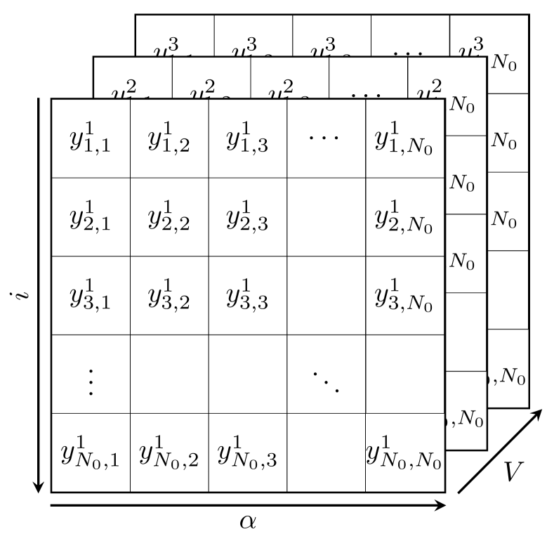
Figure 1: Visualization of the decision variables $y_{ij}^{v}$ in the Ising formulation of the routing problem.

The decision variables $y_{ij}^{v}$ are positioned as shown in Fig. 1. This picture allows us to see the operations that are taking place when summing over specific indices. As an example, consider Eq. (20). First summing over the indices $v$ and $\alpha$ corresponds to a summation over these two axes. After the summation it is easy to see that if the goal is to visit each customer/city once, then each element of the length $N_{0}$ array must be one.

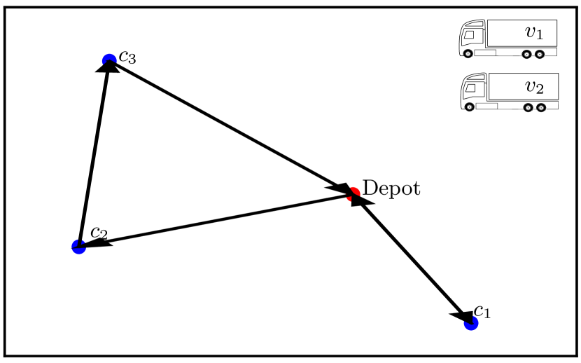
Figure 2: Visualization of a problem instance with a suggested solution. The first truck $v_{1}$ visits city $c_{2}$ and the city $c_{3}$ before returning to the depot. The second truck $v_{2}$ only visits city $c_{1}$.

One notable technicality about the formulation is that certain solutions that may be considered valid are excluded by the constraint in Eq. (21). However, the excluded solutions are physically equivalent to some allowed solution, as illustrated by the following simple example (see Fig. 2) with two trucks over three cities

$$y=\left[\begin{pmatrix}0&0&0\\ 1&0&0\\ 0&1&0\end{pmatrix},\begin{pmatrix}0&0&1\\ 0&0&0\\ 0&0&0\end{pmatrix}\right]\,,$$ (22)

and

$$y=\left[\begin{pmatrix}0&0&0\\ 1&0&0\\ 0&1&0\end{pmatrix},\begin{pmatrix}0&1&0\\ 0&0&0\\ 0&0&0\end{pmatrix}\right]\,.$$ (23)

In both cases, the two different matrices describe the routes of the two different vehicles and the order in which they visit the different customers $c_{i}$. They both represent a physically valid solution where the first truck visits first the second and then the third customer ($v_{1}:c_{2}\rightarrow c_{3}$), while the second truck goes from the depot to the first customer and then back to the depot ($v_{2}:c_{1}$). The constraint in Eq. (21), however, rules out the latter representation as it has two non-zero entries for $\alpha=2$. If we want to allow this larger set of viable representations, physically equivalent to solutions already allowed by Eq. (21), we can replace that constraint by a reformulated one,

$$H^{\prime}_{D}=D\sum_{v=1}^{V}\sum_{\alpha=1}^{N_{0}}\left(u_{\alpha}^{v}-\sum_{i=1}^{N_{0}}y_{i\alpha}^{v}\right)^{2}\,,$$ (24)

where we have introduced $N_{0}^{2}$ additional auxiliary qubits $u_{\alpha}^{v}$. Especially in the NISQ era, where quantum resources are scarce, it is important to encode the problem with as few qubits as possible. Thus we do not consider Eq. (24) a viable route for implementations, but use Eq. (21) for the simulations in Section V.

III.2 Capacity problem

The capacity constraint is of a similar nature as the constraints for the knapsack problem — both are described by an inequality constraint, which for the knapsack problem is to not add too many items to the knapsack and for the trucks to not overload the vehicles. Therefore, we can use the formulation given in Ref. Lucas (2014) to model the inequality constraint introduced by the capacities.

The knapsack problem with integer weights is the following. We have a list of $N$ objects, labeled by $i$, with the weight of each object given by $w_{i}$ and its value by $c_{i}$. The knapsack has a limited capacity of $W$. The binary decision variable $x_{i}$ denotes whether an item is contained (1) in the knapsack or not (0). The total weight of the knapsack is

$$\mathcal{W}=\sum_{i=1}^{N}w_{i}x_{i}$$ (25)

with a total value of

$$\mathcal{C}=\sum_{i=1}^{N}c_{i}x_{i}\,.$$ (26)

The NP-hard knapsack problem is to maximize $\mathcal{C}$ while satisfying the inequality constraint $\mathcal{W}\leq W$.

We can write an Ising formulation of the knapsack problem as follows. Let $z_{n}$ for $1\leq n\leq W$ be a binary variable which is 1 if the final weight of the knapsack is $n$ and 0 otherwise Lucas (2014). The Hamiltonian whose energy we seek to minimize is then

$$H =H_{A}+H_{B}\,,$$ (27)

$$H_{A} =A\left(1-\sum_{n=1}^{W}z_{n}\right)^{2}+A\left(\sum_{n=1}^{W}nz_{n}-\sum_{i=1}^{N}w_{i}x_{i}\right)^{2}\,,$$ (28)

$$H_{B} =-B\sum_{i=1}^{N}c_{i}x_{i}\,.$$ (29)

To make sure that the hard constraint is not violated, we require $0<\text{max}(|H_{B}|)<A$.

III.2.1 Reducing the number of auxiliary qubits

It is possible to reduce the number of variables required for the auxiliary variable $z_{n}$. We want to encode a variable which can take the values from 0 to $W$. Let $M\equiv\lfloor\text{log}_{2}(N)\rfloor$. We then require $M+1$ binary variables instead of $N$ binary variables:

$$\sum_{n=1}^{N}nz_{n}\rightarrow\sum_{n=0}^{M-1}2^{n}z_{n}+\left(N+1-2^{M}\right)z_{M}\,.$$ (30)

Note that if $N\neq 2^{M+1}-1$, degeneracies are possible Lucas (2014). Within this log formulation, several of the auxiliary variables can be 1, so the first part of Eq. (28) should not be included as this constraint enforces a one-hot encoding (exactly one element of the bitstring is one and the rest are zero) of the bitstrings.

We can make use of the inequality constraint given in the knapsack formulation [see Eq. (28)] to encode the capacity constraints for the HVRP. Therefore, we can neglect $H_{B}$ [see Eq. (29)] and only consider $H_{A}$ [see Eq. (28)]. Let $Q^{v}$ be the maximum capacity of vehicle $v$. The Hamiltonian then becomes

$$H_{A} =A\sum_{v}\left(1-\sum_{k=0}^{Q^{v}}z_{k}^{v}\right)^{2}+A\sum_{v}\left(\sum_{k=0}^{Q^{v}}k\cdot z_{k}^{v}-\sum_{\alpha,i}q_{i}y_{i\alpha}^{v}\right)^{2},$$ (31)

or equivalently using the log formulation,

$$H_{A} =A\sum_{v}\left(\sum_{k=0}^{M^{v}-1}2^{k}z_{k}^{v}+(Q^{v}+1-2^{M^{v}})z_{M^{v}}^{v}-\sum_{\alpha,i}q_{i}y_{i\alpha}^{v}\right)^{2}.$$ (32)

Note that by using the log trick, the decision variable $z_{k}^{v}$ switches from a one-hot encoding to a binary representation.

III.3 The full Ising Hamiltonian for the HVRP

We are now ready to write down the full Hamiltonian for the HVRP. The full Ising Hamiltonian $H_{\mathcal{C}}$ contains five terms, where the first term $H_{A}$ captures the actual optimization problem and the other terms are penalty terms to ensure that invalid configurations are penalized with a high energy:

$$H_{\mathcal{C}} =H_{A}+H_{B}+H_{C}+H_{D}+H_{E}\,,$$ (33)

$$H_{E} =E\sum_{v=1}^{V}\left(\sum_{k=0}^{M^{v}-1}2^{k}z_{k}^{v}+(Q^{v}+1-2^{M^{v}})z_{M^{v}}^{v}\right.$$

$$\left.-\sum_{\alpha=1}^{N_{0}}\sum_{i=1}^{N_{0}}q_{i}y_{i\alpha}^{v}\right)^{2}$$ (34)

For the terms $H_{A}$ to $H_{D}$, see Eqs. (18)–(21).

The formulation presented in this paper combines the capacity problem and the routing problem in one Ising Hamiltonian. Similarly, a unified approach is also attempted in Ref. Feld et al. (2019) with the difference that the authors add a constraint for clustering the customers as well. Here, by using the decision variables $y_{i\alpha}^{v}$ that indicate the position in a prospective cycle instead of $x^{v}$ that is 1 if and only if a vehicle traverses from customer $i$ to $j$, we circumvent the subtour-elimination constraint. This constraint needs to loop through all possible subtours as it is presented in Ref. Harikrishnakumar et al. (2020). Moreover, a solution obtained with our mapping does not necessarily use all the vehicles that are available. It can find the most cost efficient subset of vehicles needed to solve the task.

III.4 Resources

The required resources (qubits) for solving the HVRP with our approach can be separated into three parts. The first part comes from encoding the connections between the customers and scales with $N_{0}^{2}\cdot V$. Additionally, auxiliary qubits are required for the constraining term $H_{E}$. The overall number of qubits, $\#q$, required are

$$\#q=N_{0}^{2}\cdot V+\underbrace{\sum_{v=1}^{V}\lfloor\log_{2}Q^{v}\rfloor+1}_{H_{E}}\,.$$ (35)

Using the alternative formulation for $H_{D}$ [see Eq. (24)] adds more auxiliary qubits ($N_{0}\cdot V$), yielding

$$\#q=(N_{0}+1)N_{0}V+\sum_{v=1}^{V}\lfloor\log_{2}Q^{v}\rfloor+1\,.$$ (36)

As a comparison, we note that modern high-performance optimizers (classical computers) for the HVRP can solve problem instances with more than 1,000 customers Uchoa et al. (2017); Barman et al. (2015). For a quantum computer to solve problem instances of this size, it would need at least millions of controllable qubits. Systems of this size are likely still several years away from being realized.

IV The quantum approximate optimization algorithm

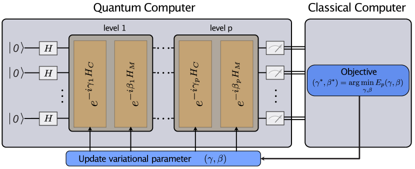
Figure 3: A schematic description of the QAOA, visualizing the interplay between the quantum device and the classical computer. The quantum computer implements a variational state formed by applying $p$ parameterized layers of operations. Each layer has operations involving the cost Hamiltonian $H_{C}$ and a mixing Hamiltonian $H_{M}$, weighted by the angles $\gamma$ and $\beta$, respectively. Measurements of the variational state and calculations of its resulting energy are used to guide the classical optimizer, which minimizes the energy in a closed-loop optimization.

The QAOA belongs to the class of hybrid quantum-classical algorithms, which combine quantum and classical processing. The closed-loop optimization of the classical and quantum devices is visualized in Fig. 3. The quantum subroutine, operating on $n$ qubits, consists of a consecutive application of two non-commuting operators defined as Farhi et al. (2014)

$$U(\gamma) \equiv e^{-i\gamma H_{\mathcal{C}}}\quad\gamma\in[0,2\pi]\,,$$ (37)

$$U(\beta) \equiv e^{-i\beta H_{M}}=\prod_{j=1}^{n}e^{-i\beta\sigma^{x}_{j}}\quad\beta\in[0,\pi]\,,$$ (38)

where $\sigma^{x}$ denotes the Pauli $X$ matrix Nielsen and Chuang (2000). This operation is analogous to the classical NOT gate. It changes the $\ket{0}$ state to the $\ket{1}$ state, and vice versa. The operator $U(\gamma)$ gives a phase rotation to each bit string depending on the cost of the string, while the mixing term $U(\beta)$ scrambles the bit strings. We call $H_{\mathcal{C}}$ the cost Hamiltonian and $H_{M}$ the mixing Hamiltonian. The bounds for $\gamma$ and $\beta$ are valid if $H_{\mathcal{C}}$ has integer eigenvalues Farhi et al. (2014). The formulation of $H_{\mathcal{C}}$ for the HVRP is given by Eq. (33).

The initial state for the algorithm is a superposition of all possible computational basis states. This superposition can be obtained by first preparing the system in the initial state $\ket{0}^{\otimes n}=\ket{00\ldots 0}$ for all qubits and then applying the Hadamard gate on each qubit:

$$\left(\tilde{H}\ket{0}\right)^{\otimes n} =\left(\frac{\ket{0}+\ket{1}}{\sqrt{2}}\right)^{\otimes n}\equiv\ket{+}^{\otimes n}\,,$$ (39)

where $\otimes$ denotes the tensor product and $\tilde{H}$ the Hadamard gate.

For any integer $p\geq 1$ and $2p$ angles $\gamma_{1}\dots\gamma_{p}\equiv\boldsymbol{\gamma}$ and $\beta_{1}\dots\beta_{p}\equiv\boldsymbol{\beta}$, we define the angle-dependent quantum state

$$\ket{\boldsymbol{\gamma,\beta}}=U(\beta_{p})U(\gamma_{p})\dots U(\beta_{1})U(\gamma_{1})\ket{+}^{\otimes n}.$$ (40)

The quantum circuit parametrized by $\boldsymbol{\gamma}$ and $\boldsymbol{\beta}$ is then optimized in a closed loop using a classical optimizer. The objective is to minimize the expectation value of the cost Hamiltonian $H_{\mathcal{C}}$ Farhi et al. (2014), i.e.,

$$(\boldsymbol{\gamma^{*},\beta^{*}}) =\underset{\boldsymbol{\gamma,\beta}}{\text{argmin }}E(\boldsymbol{\gamma,\beta})\,,$$ (41)

$$E(\boldsymbol{\gamma,\beta}) =\bra{\boldsymbol{\gamma,\beta}}H_{\mathcal{C}}\ket{\boldsymbol{\gamma,\beta}}\,.$$ (42)

The problem of calculating the energy of $2^{\#q}$ possible bit strings (solutions) is thus reduced to a variational optimization over $2p$ parameters.

V Benchmarking quantum approximate optimization for the heterogeneous vehicle routing problem

Table 1: Information about the three different problem instances used in simulations.

Problem instance	I	II	III
Number of cities	3	4	3
Number of trucks	1	1	2
Number of qubits for routing	9	16	18
Number of qubits for capacities	2	3	3
Total number of qubits	11	19	21

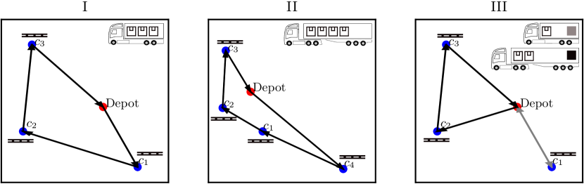
Figure 4: The three problem instances and some solutions for them obtained with low-depth QAOA. A visual representation, with correct scaling, of the three problem instances that are considered for the simulations. The optimal solution is shown. Each truck carries a predefined amount of goods and brings it to the respective customers. The pallets indicate that one item has to be carried to the customer. The crates show how much goods is carried by each truck. A color coding indicates the route assignment for problem instance III. The optimal order in which the customers are visited is indicated by arrows (the reverse order is also optimal).

In this section, we show numerical results from noise-free simulations of the QAOA applied to the HVRP. We examine three different problem instances, labelled I, II, and III, which use 11, 19, and 21 qubits, respectively. Table 1 contains information about the number of cities, available trucks, and the overall number of qubits needed to encode these problem instances in an Ising Hamiltonian using the scheme we have described in Section III. For the simulations, we consider realistic fuel consumption, gas prices, and fixed costs for each truck type, as detailed in Appendix A. A graphical representation of the problem instances is shown in Fig. 4.

For the simulations we consider two different approaches. One is to only solve for satisfying the constraints. The other is to solve the full problem, optimizing not only for feasible solutions, but for the best solution. This stepwise approach, starting with the constraints [Eqs. (20), (21), and (34)] and then including the optimization part [(Eqs. (18)–(19)], helps us understand whether some parts of the full problem contribute more to its difficulty than others.

For the first approach, finding satisfying solutions, we neglect the actual optimization part of the problem, i.e., minimizing the cost of the routing for the solution. We set the prefactors of the different parts of the Hamiltonian [Eqs. (20), (21), and (34)] to 1. The eigenvalues of the Hamiltonian are integers. This allows us to restrict the search space for $\beta$ and $\gamma$ in Eqs. (37)–(38) to $[0,\pi]$ and $[0,2\pi]$, respectively. For the full problem, we cannot make use of this simplification.

The second approach is to solve the full problem with the optimization included [Eqs. (18)–(21) and Eq. (34)]. Additionally, we rescale the cost function of the optimization [Eqs. (18)–(19)] such that it only takes values between 0 and 1. Note that for rescaling the cost, we have to evaluate the cost for each possible solution, which makes it necessary to brute-force the problem. This is only feasible for small problem instances. In a real-world application, this rescaling procedure cannot be applied and therefore it might be necessary to optimize over the penalty weights as well Roch et al. (2020); Svensson et al. (2021). The eigenvalues are not integer values anymore and therefore the entire search space for the variational parameters must be explored.

V.1 Energy landscape

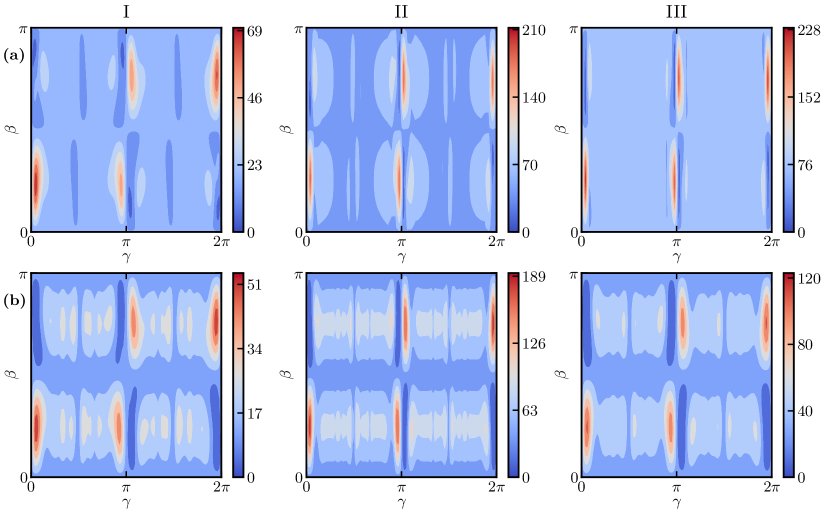
Figure 5: Energy landscapes for the three problem instances with circuit depth $p=1$. (a) The energy landscape for the full HVRP [Eqs. (18)–(21) and Eq. (34)]. The expectation value $E(\gamma,\beta)$ for the total cost depends on the classically optimized angles $\gamma$ and $\beta$. The periodicity is broken due to the non-integer eigenvalues for the cost Hamiltonian. (b) The energy landscape for the capacity constraint only [Eq. (34)]. Here, the expectation value $E(\gamma,\beta)$ describes the energy penalty for breaking the capacity constraint.

To illustrate the difficulty of finding good variational parameters for the QAOA, we show in Fig. 5 the energy landscape for $p=1$ for each problem instance considering the full problem [Fig. 5(a)] and the capacity constraint in isolation [Fig. 5(b)]. We evaluate the expectation value $E(\gamma,\beta)$ of the cost Hamiltonian on a grid $\{\gamma,\beta\}\in[0,2\pi]\times[0,\pi]$. Note that for the full problem, the entire space of variational parameters must be considered, but for this visualization we constrain it to the range mentioned.

The states with the lowest energy are marked with dark blue in Fig. 5. Each surface plot shows four distinct optima. Moreover, the variational parameters are concentrated in the same region for all three problem instances, both for the full problem and for only the capacity constraint. The range for optimal parameters narrows with increasing problem size. Similar behaviour has been observed in Ref. Streif and Leib (2020). The overall shape of the energy landscape does not change significantly with varying problem size, but the overall expectation value increases. This is not surprising, since with increasing problem size there are many more constraints to satisfy, goods to deliver, and trucks to choose from.

As discussed in Section III, the HVRP consists of two problems, a routing problem and a capacity problem. The capacity problem is analogous to the constraints of the knapsack problem Lucas (2014). To better understand the energy landscapes for the capacity part of the three problem instances shown in Fig. 5(b), we now take a closer look at the landscape of a particular knapsack problem. The problem is: given a knapsack with a maximum capacity of 5, choose from the list of items $[4,3,2,1]$ the ones that satisfy the capacity constraint. Seven qubits are needed to encode the problem, making use of the log trick introduced in Section III.2.1.

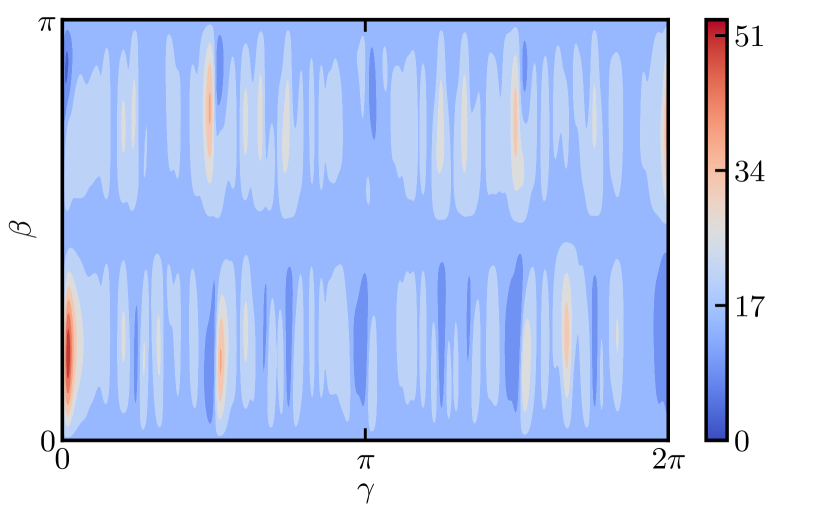
Figure 6: The energy landscape for the knapsack problem [see Eq. (28)] discussed in the main text with a circuit depth of $p=1$. The energy landscape is highly non-convex and finding the global optimum is difficult for a classical optimizer.

Figure 6 shows the energy landscape for this knapsack problem. The plot shows a rapidly oscillating energy landscape. It is clear that many optimizers will struggle to find the global optimum in this landscape. We argue that with increasing complexity of the problem instances for the HVRP, maneuvering the landscape of the capacity constraint becomes a difficult problem. In Fig. 5(b) we do not observe this behaviour yet, but this is simply due to the fact that the problem instances we consider are small (see Table 1). To obtain a landscape that is easier to handle for the classical optimizer, it might be necessary to relax the knapsack constraint or to find a different formulation to encode the capacity constraint de la Grand’rive and Hullo (2019).

V.2 Increasing the circuit depth

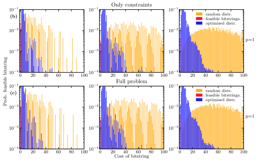
Figure 7: (a) The probability distribution of the optimized variational state (red, blue) for $p=1$. The color red shows the probability for finding a valid solution to the routing problem, i.e., a solution satisfying all constraints. The blue color indicates the overall outline of the optimized probability distribution. As a comparison, we show the probability distribution for a variational state in the $\ket{+}^{\otimes n}$ state, meaning all bitstrings are sampled with uniform probability (orange). (b) The probability distribution of the optimized variational state considering the full problem (red, blue) for $p=1$. The probability distribution is binned such that $i$ is the largest possible integer where $i\leq x$ holds, also denoted as $\lfloor x\rfloor$. That results in all feasible solutions being binned to zero and all the others being binned to integers indicating the number of constraint violations.

It has been shown that for a circuit depth of $p=1$, the QAOA cannot outperform classical optimization algorithms Farhi et al. (2014, 2020). For actual applications of the QAOA, it is therefore necessary to go to a circuit depth beyond $p=1$.

Before we investigate $p>1$, we start with the lowest possible circuit depth of $p=1$. In Fig. 7(a) and Fig. 7(b), we show a histogram of the probability distribution created by the variational circuit for finding solutions satisfying all constraints, in the cases where the cost function encodes only the constraints and the full problem, respectively. We show the probability of sampling bitstrings with a specific cost. Note that there can be several bitstrings leading to a particular cost. The probability of sampling any of the feasible bitstrings is shown in red and the rest of the optimized distribution is depicted in blue. As a comparison, we show the probability distribution for a variational state in the $\ket{+}$ state, meaning all bitstrings are sampled with uniform probability (orange). The difference between these two distributions is marginal. Thus, adding the cost terms [Eqs. (18)–(19)] to the optimization problem does not alter the overall performance of the algorithm when it comes to satisfying the constraints. This is perhaps not so surprising when considering that due to the rescaling of the cost Hamiltonian, the costs not associated with constraints impact the overall shape of the energy landscape less.

The optimized probability distribution is shifted to the left compared to the random distribution. Thus, sampling from the optimized variational state gives solutions with overall lower energy compared to random sampling of bitstrings. Moreover, for the small problem instance with 11 qubits, it is possible to sample valid bitstrings with a probability of approximately 3 %. For the 19- and 21-qubit problem instances, the probability of sampling a valid bitstring is about an order of magnitude less. This is not surprising since we are limiting the algorithm to a shallow circuit depth.

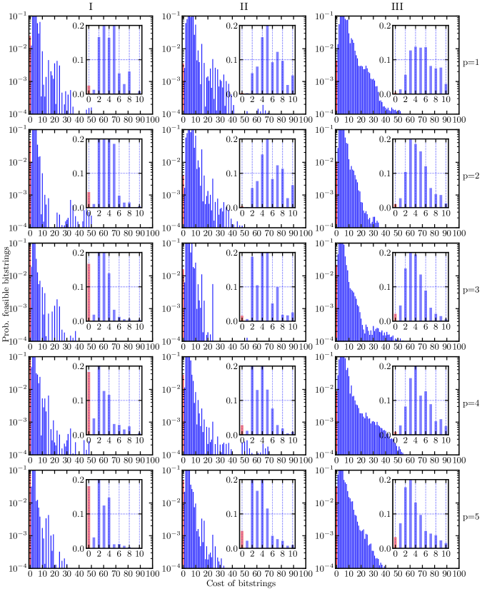
Figure 8: The probability distribution of the variational state $\ket{\boldsymbol{\gamma,\beta}}$ for the 11- (left), 19- (middle) and 21-qubit (right) problem instances as a function of the circuit depth $p$ for obtaining feasible tours. The circuit depth increases from top $p=1$ to bottom $p=5$ and shifts to lower-energy eigenstates with increasing circuit depth. The probability of sampling bitstrings that encode the optimal solution is marked with red. The simulations were conducted with the classical optimizer basinhopping with the local optimizer BFGS (see Section V.3).

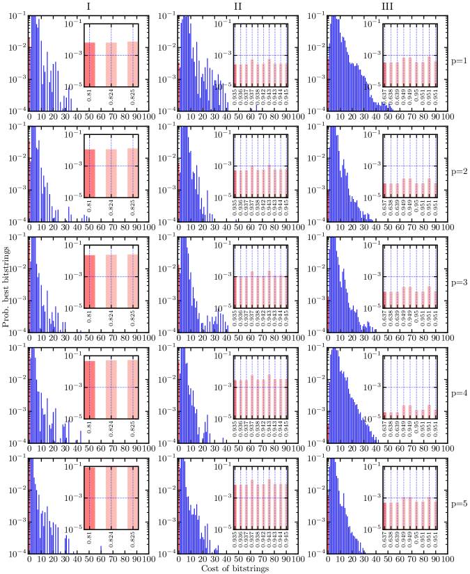
Figure 9: The probability distribution of the variational state $\ket{\boldsymbol{\gamma,\beta}}$ for the 11- (left), 19- (middle), and 21-qubit (right) problem instances as a function of the circuit depth $p$ for finding the best tour. The circuit depth increases from top $p=1$ to bottom $p=5$ and shifts to lower-energy eigenstates with increasing circuit depth. The probability of sampling the best bitstrings is marked with red. The binning is done in the same way as in Fig. 7(b). The inset shows the probability for sampling any of the two best bitstrings (dark red, leftmost bin) and the probabilities for sampling any of the other feasible bitstrings (light red). The simulations were conducted with the classical optimizer basinhopping with the local optimizer BFGS (see Section V.3).

Next, we go to a circuit depth above $1$. Here we consider in Fig. 8 and Fig. 9 finding feasible solutions and the best solutions, respectively. We shows how the variational state changes with increasing circuit depth from $p=1$ to $p=5$ for the three problem instances [see Fig. 4]. Additionally, we show for Fig. 8 an inset focusing on the low-energy part of the distribution of the variational state and for Fig. 9 an inset focusing on all feasible bitstrings. Again, the bitstrings we are aiming to sample are marked in red and the rest of the optimized distribution is depicted in blue.

For the 11-qubit instance, the probability of sampling a valid bitstring reaches values up to 18 % for $p=5$. For the slightly larger instances (19 and 21 qubits), the probability of sampling a valid bitstring does not exceed 5 % (see Fig. 8). For the more difficult problem of actually finding the optimal tour (not just a feasible tour), the probability drops to 9 % for the 11-qubit instance, while for the 19- and 21-qubit instances the probability of sampling the ideal bitstring is below 1 % (see Fig. 9).

The inset in Fig. 9 shows that the algorithm cannot distinguish between the different feasible solutions and thus fails to optimize for the best solution. This might be due to the very small energy gap between the lowest and next lowest energy eigenstate, which is an artifact of the rescaling of the cost we introduced earlier. The point of this rescaling is to ensure that all feasible solutions have lower energy than any solution violating any constraint. Rigorous hyperparameter optimization might be necessary to weight the cost and the constraints to circumvent the problems introduced by the chosen rescaling Roch et al. (2020).

The probability of sampling bitstrings with low cost increases with increasing circuit depth, meaning that the probability distribution shifts to lower-energy eigenstates. This trend is visible in Fig. 8 and Fig. 9 as the probability distribution shifts increasingly to the left with increasing depth. It might be possible with increasing circuit depth to obtain higher probabilities of sampling optimal solutions at the expense of optimizing more variational parameters. This is in accordance with the theory of adiabatic quantum optimization (AQO) — the performance of the algorithm becomes better with more variational parameters. The drawback is that the optimization problem becomes increasingly difficult and time-consuming. It is therefore important to select a good optimization method.

V.3 Performance comparison of classical optimizers

Optimizers for finding the variational parameters play an important role in the context of VQAs. Much of the current research aims to find optimizers that perform well on these quantum circuits Barkoutsos et al. (2020); Kübler et al. (2019); Spall (1992); Verdon et al. (2019). There is a rich literature on optimizers for variational circuits proposing different optimizers for different problems Cerezo et al. (2020); Lavrijsen et al. (2020).In the following, we analyze the performance of simulations using four different well-known optimizers: Nelder-Mead Nelder and Mead (1965), Powell Powell (1964), differential evolution Storn and Price (1996), and basinhopping Wales and Doye (1998). The selected optimizers work differently: some use global search mechanisms consisting of multiple random initial guesses while others use only a single random initial guess as a starting point for the optimization. These characteristics are crucial to understand why the performance of the optimizer varies.

The Nelder-Mead method uses a geometrical shape called a simplex to search the function space. With each step of the optimization, the simplex shifts, ideally, towards the region with a minimum. The Nelder-Mead algorithm belongs to the class of gradient-free optimizers. The Powell optimzer works for non-differentiable functions; no derivatives are needed for the optimization. The method minimises the function by a bi-directional search along each search vector. The initial search vectors are typically the normals aligned to each axis. The differential evolution algorithm is stochastic in nature and does not rely on derivatives to find the minimum. This algorithm often requires larger numbers of function evaluations than conventional gradient-based techniques. The basinhopping optimization algorithm is a two-phase method, which couples a global search algorithm with a local minimization at each step. For the simulations here (including in the preceding sections), we used the BFGS algorithm Frédéric Bonnans et al. (2006) as a local optimizer. This framework has been proven useful for hard nonlinear optimization problems with multiple variables Olson et al. (2012).

To speed up the optimization routines, we use the optimized parameters from $p-1$ as an intial guess for the optimization of the variational circuits for $p>1$, as well as the optimized parameters from the 11-qubit problem instance as an initial guess for the 19- and 21-qubit instances. The concentration of variational parameters for the QAOA has been observed by many researchers Streif and Leib (2020); Akshay et al. (2021). It has been shown for a circuit depth of $p=1,2$ that the variational parameters for small problem instances can be used to infer parameters for larger problem instances Akshay et al. (2021). This can significantly speed up the optimization of the QAOA.

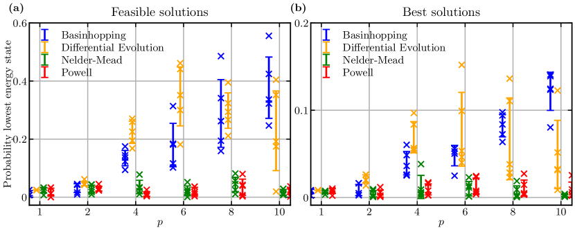
Figure 10: Comparing different optimizers for the HVRP on the 11-qubit problem instance shown in Fig. 4. A probability of 1 means that a feasible bitstring is always sampled. (a) Success probability for finding a valid solution with increasing circuit depth $p$. (b) Success probability for finding the best solution with increasing circuit depth $p$.

In Fig. 10(a), we show the success probability of finding a viable bitstring as a function of the circuit depth $p$ for the 11-qubit problem instance. Similarly, we show the success probability of sampling one of the two optimal tours as a function of the circuit depth $p$ in Fig. 10(b). One of the optimal tours is shown in Fig. 4. The other optimal solution is following the same path in reverse order.

The results show in Fig. 10 clearly favours the optimizers basinhopping and differential evolution. They perform significantly better than the Nelder-Mead and Powell optimization algorithms. This difference in performance might be due to the global optimization routine that these latter two algorithms use to find the optima. The performance of the Nelder-Mead algorithm strongly depends on the initial simplex and the simplex is usually randomly generated. Depending on the starting point, the performance can vary, but it usually cannot compete with the solution quality of the basinhopping or differential-evolution algorithms.

V.4 Runtime comparison of the classical optimizers

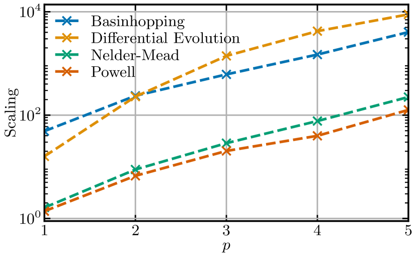
Figure 11: Runtime comparison for the four classical optimizers tested in this work. The plot shows the runtime as a function of circuit depth $p$.

For applications it is also important to understand the scaling of the runtime of the optimization routine with increasing circuit depth. Here we benchmark the classical optimizers from the preceding subsection on this measure. The result is shown in Fig. 11.

We see that the optimizers basinhopping and differential evolution need roughly one order of magnitude more time for the optimization than the Nelder-Mead and Powell algorithms. This is due to the many circuit queries the former optimizers have to perform. The tradeoff between the runtime of the algorithm and its performance becomes evident, as the slowest optimizers in terms of runtime performed best in terms of success probability (see Fig. 10). Moreover, the linear increase for all optimizers on the semi-log scale in Fig. 11 indicates that the amount of time needed for the optimzation scales exponentially with $p$. However, further investigation is needed to confirm this statement. It might become a difficult problem to tackle when a circuit depth beyond $p=20$ is considered.

As mentioned earlier, researchers are already investigating how the optimization could be simplified or circumvented completely Streif and Leib (2020); Akshay et al. (2021). The results here further underlines the importance of such research.

VI Conclusion

We have derived an Ising formulation for the heterogeneous vehicle routing problem (HVRP) under consideration of all relevant constraints, enabling this problem to be solved on a quantum computer. In our formulation, the number of qubits needed to encode a problem instance scales quadratically with the number of customers. Therefore, quantum computers will need to have at least millions of qubits to use our suggested encoding scheme to solve problem instances that are at the limit of what today’s classical high-performance optimizers can solve. A quantum advantage could still be had with fewer qubits for smaller problems if they could be solved faster on a quantum computer than on a classical one, but the present work did not give indications of such speed-ups for small problems.

We simulated solving small instances of the HVRP and with the quantum approximate optimization algorithm (QAOA). We considered three distinct problems, requiring 11, 19, and 21 qubits, respectively. We investigated the performance of the algorithm with respect to two design choices: the classical optimizer and the depth $p$ of the quantum circuit.

For the choice of optimizer, we found that the basinhopping and differential-evolution algorithms seem well suited to optimize the variational parameters of the quantum circuit. However, this performance came at the expense of comparably long optimization times. Furthermore, our data indicates that the optimization time needed to find suitable angles for the variational quantum circuit increases exponentially with $p$, but further investigation is needed to verify this scaling.

We have seen that routing with additional capacity constraints is a difficult problem for the hybrid quantum-classical approach to handle. The problem becomes more evident when isolating the inequality constraint. Then we can see that the energy landscape has multiple scattered local minima. In future work, one might want to consider a different formulation for the capacity constraint de la Grand’rive and Hullo (2019).

Moreover, Fig. 9 shows that the QAOA fails to distinguish solutions that satisfy all constraints but differ in cost. This failure may be due to the small energy gap between the different feasible solutions and could be circumvented by restating the problem such that feasible solutions are separated by larger energy gaps. One way of achieving this goal is to conduct a rigorous hyperparameter optimization to weight the cost and the constraints accordingly. Similar ideas were explored for the knapsack problem in Ref. Roch et al. (2020).

VII Outlook

The classical optimization procedure is a central component in all variational algorithms and key to their success. Therefore, finding new optimizers is one interesting area of research. Several works have investigated machine-learning-based optimizers Verdon et al. (2019); Yao et al. (2020); Garcia-Saez and Riu (2019). A study of such optimizers for the HVRP could boost the performance of the algorithm.

Even though we assumed a noise-free system, the performance is not competitive with modern high-performance heuristics Perron and Furnon ; Uchoa et al. (2017) which can solve instances with more than 1,000 customers. Such optimizers are not limited in the number of decision variables, but rather by the running time for the optimization. However, the problems we considered are too small for a meaningful comparison. Furthermore, the assumption of a noise-free system does not hold for NISQ computers and a decrease in performance can be expected if the algorithm is executed on such a device Preskill (2018); Streif et al. (2021). An interesting topic for future work would be to investigate the HVRP in combination with QAOA under the assumption of a noisy system. Moreover, running small problems on an actual quantum computer could give a better view on the applicability of the QAOA to the HVRP and its competitiveness with classical heuristics.

In Fig. 6, we could see that the knapsack constraint creates an energy landscape with rapidly oscillating local minima. This makes it difficult for many optimizers to find a good approximate solution. It would be interesting to investigate why this particular problem is difficult and if it is possible to relax the knapsack constraint or reformulate it such that the optimization landscape becomes easier to maneuver.

Furthermore, the QAOA can be expanded to the quantum alternating operator ansatz Hadfield et al. (2019). Investigating different mixer Hamiltonians for the HVRP could lead to a better overall performance. Ideally, the mixer Hamiltonian would provide a framework that keeps the algorithm in the subspace of allowed solutions Wang et al. (2020). Currently, the standard mixer Hamiltonian used in this work makes the algorithms explore every possible bitstring.

Finally, we note that for real-world applications it might be necessary to consider multiple depots. Therefore, another avenue to explore are more Ising formulations that allow for solving different variations of VRPs.

Appendix A Additional information for the simulation of the QAOA

The information used to determine the fixed and variable cost for the QAOA simulations in this work is shown in Table 2. The table shows the fuel consumption and cost per 100 km, the price of the chassis, and loading capacity Ghandriz (2018) for the two truck types we consider in Fig. 4: a rigid truck (rt) and a tractor–semitrailer (ts).

Table 2: Fuel consumption $f$ and corresponding cost $c_{\rm road}$ per 100km, the price $c_{\rm chass}$ of the chassis as well as the loading capacity Ghandriz (2018) for each of the two different truck types considered in the simulations of this paper. Note that the loading capacity does not take into account the size or weight of items that can be carried by the truck. The information in this table is used to determine the variable and fixed costs in Eqs. 18 and 19.

	rt	ts
$f$ [l/100 km]	28.6 sit (2020)	34.5 Clausen et al. (2015)
$c_{\rm road}$ [€/100 km]	34.32	41.4
$c_{\rm chass}[$€$]$	75,000	150,000
$m_{\rm max}$ [items]	3	4

References

- Shor (2002) P. Shor, “Algorithms for quantum computation: discrete logarithms and factoring,” in Proceedings 35th Annual Symposium on Foundations of Computer Science (IEEE Comput. Soc. Press, 2002) pp. 124–134.
- Harrow et al. (2009) A. W. Harrow, A. Hassidim, and S. Lloyd, “Quantum Algorithm for Linear Systems of Equations,” Physical Review Letters 103, 150502 (2009), arXiv:0811.3171 .
- Montanaro (2016) A. Montanaro, “Quantum algorithms: An overview,” npj Quantum Information 2, 15023 (2016), arXiv:1511.04206 .
- Wendin (2017) G. Wendin, “Quantum information processing with superconducting circuits: a review.” Reports on progress in physics. Physical Society (Great Britain) 80, 106001 (2017), arXiv:1610.02208 .
- Bharti et al. (2021) K. Bharti, A. Cervera-Lierta, T. H. Kyaw, T. Haug, S. Alperin-Lea, A. Anand, M. Degroote, H. Heimonen, J. S. Kottmann, T. Menke, W.-K. Mok, S. Sim, L.-C. Kwek, and A. Aspuru-Guzik, “Noisy intermediate-scale quantum (NISQ) algorithms,” (2021), arXiv:2101.08448 .
- Arute et al. (2019) F. Arute et al., “Quantum supremacy using a programmable superconducting processor,” Nature 574, 505 (2019), arXiv:1911.00577 .
- Bruzewicz et al. (2019) C. D. Bruzewicz, J. Chiaverini, R. McConnell, and J. M. Sage, “Trapped-ion quantum computing: Progress and challenges,” Applied Physics Reviews 6, 021314 (2019), arXiv:1904.04178 .
- Kjaergaard et al. (2020) M. Kjaergaard, M. E. Schwartz, J. Braumüller, P. Krantz, J. I.-J. Wang, S. Gustavsson, and W. D. Oliver, “Superconducting Qubits: Current State of Play,” Annual Review of Condensed Matter Physics 11, 369–395 (2020), arXiv:1905.13641 .
- Zhong et al. (2020) H.-S. Zhong, H. Wang, Y.-H. Deng, M.-C. Chen, L.-C. Peng, Y.-H. Luo, J. Qin, D. Wu, X. Ding, Y. Hu, P. Hu, X.-Y. Yang, W.-J. Zhang, H. Li, Y. Li, X. Jiang, L. Gan, G. Yang, L. You, Z. Wang, L. Li, N.-L. Liu, C.-Y. Lu, and J.-W. Pan, “Quantum computational advantage using photons,” Science 370, 1460 (2020), arXiv:2012.01625 .
- Farhi et al. (2014) E. Farhi, J. Goldstone, and S. Gutmann, “A Quantum Approximate Optimization Algorithm,” (2014), arXiv:1411.4028 .
- Koç et al. (2016) Ç. Koç, T. Bektaş, O. Jabali, and G. Laporte, “Thirty years of heterogeneous vehicle routing,” European Journal of Operational Research, 249, 1–21 (2016).
- Preskill (2018) J. Preskill, “Quantum Computing in the NISQ era and beyond,” Quantum 2, 79 (2018), arXiv:1801.00862 .
- Hauke et al. (2020) P. Hauke, H. G. Katzgraber, W. Lechner, H. Nishimori, and W. D. Oliver, “Perspectives of quantum annealing: Methods and implementations,” Reports on Progress in Physics 83, 054401 (2020), arXiv:1903.06559 .
- Golden et al. (2008) B. Golden, S. Raghavan, and E. Wasil, “The vehicle routing problem: Latest advances and new challenges,” Operations Research/ Computer Science Interfaces Series 43, 3–27 (2008).
- Caunhye et al. (2012) A. M. Caunhye, X. Nie, and S. Pokharel, “Optimization models in emergency logistics: A literature review,” Socio-Economic Planning Sciences 46, 4–13 (2012).
- Ghandriz et al. (2021) T. Ghandriz, B. Jacobson, M. Islam, J. Hellgren, and L. Laine, “Transportation-Mission-Based Optimization of Heterogeneous Heavy-Vehicle Fleet Including Electrified Propulsion,” Energies 14, 3221 (2021).
- Lenstra and Kan (1981) J. K. Lenstra and A. H. Kan, “Complexity of vehicle routing and scheduling problems,” Networks 11, 221–227 (1981).
- Laporte et al. (2014) G. Laporte, S. Ropke, and T. Vidal, “Chapter 4: Heuristics for the Vehicle Routing Problem,” in Vehicle Routing, September (Society for Industrial and Applied Mathematics, Philadelphia, PA, 2014) pp. 87–116.
- Tavares et al. (2009) L. G. Tavares, H. S. Lopes, and C. R. Lima, “Construction and improvement heuristics applied to the capacitated vehicle routing problem,” 2009 World Congress on Nature and Biologically Inspired Computing, NABIC 2009 - Proceedings , 690–695 (2009).
- Hwang et al. (1999) C. P. Hwang, B. Alidaee, and J. D. Johnson, “A tour construction heuristic for the travelling salesman problem,” Journal of the Operational Research Society 50, 797–809 (1999).
- Van Breedam (1995) A. Van Breedam, “Improvement heuristics for the Vehicle Routing Problem based on simulated annealing,” European Journal of Operational Research 86, 480–490 (1995).
- Brandstätter and Reimann (2018) C. Brandstätter and M. Reimann, “Performance analysis of a metaheuristic algorithm for the line-haul feeder vehicle routing problem,” Journal on Vehicle Routing Algorithms 1, 121–138 (2018).
- Clarke and Wright (1964) G. Clarke and J. W. Wright, “Scheduling of Vehicles from a Central Depot to a Number of Delivery Points,” Operations Research 12, 568–581 (1964).
- Lougee (2003) R. Lougee, “The common optimization interface for operations research: Promoting open-source software in the operations research community,” IBM Journal of Research and Development 47, 57–66 (2003).
- Groër et al. (2010) C. Groër, B. Golden, and E. Wasil, “A library of local search heuristics for the vehicle routing problem,” Math. Prog. Comp 2, 79–101 (2010).
- (26) L. Perron and V. Furnon, “Or-tools,” .
- Baldacci and Mingozzi (2009) R. Baldacci and A. Mingozzi, “A unified exact method for solving different classes of vehicle routing problems,” Mathematical Programming 120, 347–380 (2009).
- Jazaeri et al. (2019) F. Jazaeri, A. Beckers, A. Tajalli, and J. M. Sallese, “A Review on Quantum Computing: From Qubits to Front-end Electronics and Cryogenic MOSFET Physics,” in Proceedings of the 26th International Conference ”Mixed Design of Integrated Circuits and Systems”, MIXDES 2019 (IEEE, 2019) pp. 15–25, arXiv:1908.02656v1 .
- Pino et al. (2021) J. M. Pino, J. M. Dreiling, C. Figgatt, J. P. Gaebler, S. A. Moses, M. S. Allman, C. H. Baldwin, M. Foss-Feig, D. Hayes, K. Mayer, C. Ryan-Anderson, and B. Neyenhuis, “Demonstration of the trapped-ion quantum CCD computer architecture,” Nature 592, 209 (2021), arXiv:2003.01293 .
- Mooney et al. (2021) G. J. Mooney, G. A. L. White, C. D. Hill, and L. C. L. Hollenberg, “Whole-device entanglement in a 65-qubit superconducting quantum computer,” (2021), arXiv:2102.11521 .
- Blinov et al. (2021) S. Blinov, B. Wu, and C. Monroe, “Comparison of Cloud-Based Ion Trap and Superconducting Quantum Computer Architectures,” (2021), arXiv:2102.00371 .
- Pogorelov et al. (2021) I. Pogorelov, T. Feldker, C. D. Marciniak, L. Postler, G. Jacob, O. Krieglsteiner, V. Podlesnic, M. Meth, V. Negnevitsky, M. Stadler, B. Höfer, C. Wächter, K. Lakhmanskiy, R. Blatt, P. Schindler, and T. Monz, “A compact ion-trap quantum computing demonstrator,” PRX Quantum 2, 020343 (2021), arXiv:2101.11390 .
- Wu et al. (2021) Y. Wu et al., “Strong quantum computational advantage using a superconducting quantum processor,” (2021), arXiv:2106.14734 .
- Kandala et al. (2017) A. Kandala, A. Mezzacapo, K. Temme, M. Takita, M. Brink, J. M. Chow, and J. M. Gambetta, “Hardware-efficient variational quantum eigensolver for small molecules and quantum magnets,” Nature 549, 242–246 (2017), arXiv:1704.05018 .
- Cerezo et al. (2020) M. Cerezo, A. Arrasmith, R. Babbush, S. C. Benjamin, S. Endo, K. Fujii, J. R. McClean, K. Mitarai, X. Yuan, L. Cincio, and P. J. Coles, “Variational Quantum Algorithms,” arXiv, (2020), arXiv:2012.09265 .
- Stamatopoulos et al. (2020) N. Stamatopoulos, D. J. Egger, Y. Sun, C. Zoufal, R. Iten, N. Shen, and S. Woerner, “Option pricing using quantum computers,” Quantum 4, 291 (2020), arXiv:1905.02666 .
- Vikstål et al. (2020) P. Vikstål, M. Grönkvist, M. Svensson, M. Andersson, G. Johansson, and G. Ferrini, “Applying the quantum approximate optimization algorithm to the tail-assignment problem,” Physical Review Applied 14, 034009 (2020), arXiv:1912.10499 .
- Braine et al. (2021) L. Braine, D. J. Egger, J. Glick, and S. Woerner, “Quantum Algorithms for Mixed Binary Optimization Applied to Transaction Settlement,” IEEE Transactions on Quantum Engineering, 2, 3101208 (2021), arXiv:1910.05788 .
- Choi et al. (2019) H. Choi, K. S. Sohn, M. Pyo, K. C. Chung, and H. Park, “Predicting the Electrochemical Properties of Lithium-Ion Battery Electrode Materials with the Quantum Neural Network Algorithm,” Journal of Physical Chemistry C 123, 4682–4690 (2019).
- Egger et al. (2021) D. J. Egger, C. Gambella, J. Marecek, S. McFaddin, M. Mevissen, R. Raymond, A. Simonetto, S. Woerner, and E. Yndurain, “Quantum Computing for Finance: State-of-the-Art and Future Prospects,” IEEE Transactions on Quantum Engineering, 1, 3101724 (2021), arXiv:2006.14510 .
- Syrichas and Crispin (2017) A. Syrichas and A. Crispin, “Large-scale vehicle routing problems: Quantum Annealing, tunings and results,” Computers and Operations Research 87, 52–62 (2017).
- Feld et al. (2019) S. Feld, C. Roch, T. Gabor, C. Seidel, F. Neukart, I. Galter, W. Mauerer, and C. Linnhoff-Popien, “A Hybrid Solution Method for the Capacitated Vehicle Routing Problem Using a Quantum Annealer,” Frontiers in ICT 6, 13 (2019), arXiv:1811.07403 .
- Harikrishnakumar et al. (2020) R. Harikrishnakumar, S. Nannapaneni, N. H. Nguyen, J. E. Steck, and E. C. Behrman, “A Quantum Annealing Approach for Dynamic Multi-Depot Capacitated Vehicle Routing Problem,” (2020), arXiv:2005.12478 .
- Utkarsh et al. (2020) Utkarsh, B. K. Behera, and P. K. Panigrahi, “Solving Vehicle Routing Problem Using Quantum Approximate Optimization Algorithm,” (2020), arXiv:2002.01351 .
- Harrigan et al. (2021) M. P. Harrigan et al., “Quantum approximate optimization of non-planar graph problems on a planar superconducting processor,” Nature Physics 17, 332–336 (2021), arXiv:2004.04197 .
- Bengtsson et al. (2020) A. Bengtsson, P. Vikstål, C. Warren, M. Svensson, X. Gu, A. F. Kockum, P. Krantz, C. Križan, D. Shiri, I.-M. Svensson, G. Tancredi, G. Johansson, P. Delsing, G. Ferrini, and J. Bylander, “Improved Success Probability with Greater Circuit Depth for the Quantum Approximate Optimization Algorithm,” Physical Review Applied 10, 34010 (2020).
- Abrams et al. (2020) D. M. Abrams, N. Didier, B. R. Johnson, M. P. Silva, and C. A. Ryan, “Implementation of XY entangling gates with a single calibrated pulse,” Nature Electronics 3, 744–750 (2020).
- Willsch et al. (2020) M. Willsch, D. Willsch, F. Jin, H. De Raedt, and K. Michielsen, “Benchmarking the quantum approximate optimization algorithm,” Quantum Information Processing 19, 197 (2020), arXiv:1907.02359 .
- Otterbach et al. (2017) J. S. Otterbach et al., “Unsupervised Machine Learning on a Hybrid Quantum Computer,” arXiv, (2017), arXiv:1712.05771 .
- Ising (1925) E. Ising, “Beitrag zur Theorie des Ferromagnetismus,” Zeitschrift für Physik 31, 253 (1925).
- Brush (1967) S. G. Brush, “History of the Lenz-Ising Model,” Reviews of Modern Physics 39, 883 (1967).
- Lucas (2014) A. Lucas, “Ising formulations of many NP problems,” Frontiers in Physics 2, 5 (2014), arXiv:1302.5843 .
- Roch et al. (2020) C. Roch, A. Impertro, T. Phan, T. Gabor, S. Feld, and C. Linnhoff-Popien, “Cross entropy hyperparameter optimization for constrained problem hamiltonians applied to QaoA,” Proceedings - 2020 International Conference on Rebooting Computing, ICRC 2020 , 50–57 (2020), arXiv:2003.05292 .
- Uchoa et al. (2017) E. Uchoa, D. Pecin, A. Pessoa, M. Poggi, T. Vidal, and A. Subramanian, “New benchmark instances for the Capacitated Vehicle Routing Problem,” European Journal of Operational Research 257, 845–858 (2017).
- Barman et al. (2015) S. E. Barman, P. Lindroth, and A.-B. Strömberg, “Modeling and Solving Vehicle Routing Problems with Many Available Vehicle Types,” in Optimization, Control, and Applications in the Information Age, edited by A. Migdalas and A. Karakitsiou (Springer International Publishing, Cham, 2015) pp. 113–138.
- Nielsen and Chuang (2000) M. A. Nielsen and I. L. Chuang, Quantum computation and quantum information (Cambridge University Press, 2000).
- Svensson et al. (2021) M. Svensson, M. Andersson, M. Grönkvist, P. Vikstål, D. Dubhashi, G. Ferrini, and G. Johansson, “A Heuristic Method to solve large-scale Integer Linear Programs by combining Branch-and-Price with a Quantum Algorithm,” (2021), arXiv:2103.15433 .
- Streif and Leib (2020) M. Streif and M. Leib, “Training the quantum approximate optimization algorithm without access to a quantum processing unit,” Quantum Science and Technology 5, 034008 (2020), arXiv:1908.08862 .
- de la Grand’rive and Hullo (2019) P. D. de la Grand’rive and J.-F. Hullo, “Knapsack Problem variants of QAOA for battery revenue optimisation,” (2019), arXiv:1908.02210 .
- Farhi et al. (2020) E. Farhi, D. Gamarnik, and S. Gutmann, “The Quantum Approximate Optimization Algorithm Needs to See the Whole Graph: Worst Case Examples,” (2020), arXiv:2005.08747 .
- Barkoutsos et al. (2020) P. K. Barkoutsos, G. Nannicini, A. Robert, I. Tavernelli, and S. Woerner, “Improving Variational Quantum Optimization using CVaR,” Quantum 4, 256 (2020), arXiv:1907.04769 .
- Kübler et al. (2019) J. M. Kübler, A. Arrasmith, L. Cincio, and P. J. Coles, “An adaptive optimizer for measurement-frugal variational algorithms,” Quantum 4, 263 (2019), arXiv:1909.09083 .
- Spall (1992) J. C. Spall, IEEE Transactions on Automatic Control, Tech. Rep. 3 (1992).
- Verdon et al. (2019) G. Verdon, M. Broughton, J. R. McClean, K. J. Sung, R. Babbush, Z. Jiang, H. Neven, and M. Mohseni, “Learning to learn with quantum neural networks via classical neural networks,” (2019), arXiv:1907.05415 .
- Lavrijsen et al. (2020) W. Lavrijsen, A. Tudor, J. Muller, C. Iancu, and W. De Jong, “Classical Optimizers for Noisy Intermediate-Scale Quantum Devices,” in Proceedings - IEEE International Conference on Quantum Computing and Engineering, QCE 2020 (2020) pp. 267–277, arXiv:2004.03004 .
- Nelder and Mead (1965) J. A. Nelder and R. Mead, “A Simplex Method for Function Minimization,” The Computer Journal 7, 308–313 (1965).
- Powell (1964) M. J. D. Powell, “An efficient method for finding the minimum of a function of several variables without calculating derivatives,” The Computer Journal 7, 155–162 (1964).
- Storn and Price (1996) R. Storn and K. Price, “Differential Evolution – A Simple and Efficient Heuristic for Global Optimization over Continuous Spaces,” Journal of Global Optimization (1996).
- Wales and Doye (1998) D. Wales and J. Doye, “Global Optimization by Basin-Hopping and the Lowest Energy Structures of Lennard-Jones Clusters Containing up to 110 Atoms,” The Journal of Physical Chemistry A 101, 5111–5116 (1998), arXiv:9803344 [cond-mat] .
- Frédéric Bonnans et al. (2006) J. Frédéric Bonnans, J. Charles Gilbert, C. Lemaréchal, and C. A. Sagastizábal, Numerical Optimization: Theoretical and Practical Aspects (2006) pp. 1–494.
- Olson et al. (2012) B. Olson, I. Hashmi, K. Molloy, and A. Shehu, “Basin Hopping as a General and Versatile Optimization Framework for the Characterization of Biological Macromolecules,” Advances in Artificial Intelligence 2012, 674832 (2012).
- Akshay et al. (2021) V. Akshay, D. Rabinovich, E. Campos, and J. Biamonte, “Parameter concentrations in quantum approximate optimization,” Physical Review A 104, L010401 (2021), arXiv:2103.11976 .
- Yao et al. (2020) J. Yao, M. Bukov, and L. Lin, “Policy Gradient based Quantum Approximate Optimization Algorithm,” Proceedings of Machine Learning Research 107, 1–30 (2020), arXiv:2002.01068 .
- Garcia-Saez and Riu (2019) A. Garcia-Saez and J. Riu, “Quantum Observables for continuous control of the Quantum Approximate Optimization Algorithm via Reinforcement Learning,” (2019), arXiv:1911.09682 .
- Streif et al. (2021) M. Streif, M. Leib, F. Wudarski, E. Rieffel, and Z. Wang, “Quantum algorithms with local particle-number conservation: Noise effects and error correction,” Physical Review A 103, 042412 (2021), arXiv:2011.06873 .
- Hadfield et al. (2019) S. Hadfield, Z. Wang, B. O’Gorman, E. Rieffel, D. Venturelli, and R. Biswas, “From the Quantum Approximate Optimization Algorithm to a Quantum Alternating Operator Ansatz,” Algorithms 12, 34 (2019), arXiv:1709.03489 .
- Wang et al. (2020) Z. Wang, N. C. Rubin, J. M. Dominy, and E. G. Rieffel, “XY mixers: Analytical and numerical results for the quantum alternating operator ansatz,” Physical Review A 101, 012320 (2020), arXiv:1904.09314 .
- Ghandriz (2018) T. Ghandriz, Transportation Mission Based Optimization of Heavy Vehicle Fleets including Propulsion Tailoring, Licentiate thesis, Chalmers University of Technology (2018).
- sit (2020) “Average fuel consumption in Australia,” (2020).
- Clausen et al. (2015) U. Clausen, H. Friedrich, C. Thaller, and C. Geiger, Commercial Transport: Proceedings of the 2nd Interdisciplinary Conference on Production Logistics and Traffic 2015, Lecture Notes in Logistics (Springer International Publishing, 2015).
- fue (2020) “Germany Diesel prices, 09-Mar-2020,” (2020).