Analysis of the gradual transition from the near to the far field in single-slit diffraction

Abstract

In Optics it is common to split up the formal analysis of diffraction according to two convenient approximations, in the near and far fields (also known as the Fresnel and Fraunhofer regimes, respectively). Within this scenario, geometrical optics, the optics describing the light phenomena observable in our everyday life, is introduced as the short-wavelength limit of near-field phenomena, assuming that the typical size of the aperture (or obstacle) that light is incident on is much larger than the light wavelength. With the purpose to provide an alternative view on how geometrical optics fits within the context of the diffraction theory, particularly how it emerges, the transition from the near to the far field is revisited here both analytically and numerically. Accordingly, first this transition is investigated in the case of Gaussian beam diffraction, since its full analyticity paves the way for a better understanding of the paradigmatic (and typical) case of diffraction by sharp-edged single slits. This latter case is then tackled both analytically, by means of some insightful approximations and guesses, and numerically. As it is shown, this analysis makes explicit the influence of the various parameters involved in diffraction processes, such as the typical size of the input (diffracted) wave or its wavelength, or the distance between the input and output planes. Moreover, analytical expressions have been determined for the critical turnover value of the slit width that separates typical Fraunhofer diffraction regimes from the behaviors eventually leading to the geometrical optics limit, finding a good agreement with both numerically simulated results and experimental data extracted from the literature.

1 Introduction

Due to the wave nature of light, and more specifically the phenomenon of diffraction, the intensity distribution observed behind a sharp opening is not homogeneous. Consider the paradigmatic case of a very long rectangular slit [1, 2]. As is well known [2], the intensity distribution generated by this slit exhibits a series of alternating bright and dark light fringes aligned parallel to the slit. Accordingly, when observed along the transverse direction (perpendicular to the fringes), the profile of this intensity distribution is described by a succession of maxima and minima, with the maxima decreasing in intensity from the center of the pattern to the sides. This phenomenon is observable whenever the wavelength of the incident light is comparable with the dimensions of the slit (in this case, with respect to its width along the transverse direction). Furthermore, it is also known [3] that, as the projection screen where the intensity is observed moves further away from the slit, the intensity distribution gradually changes from a highly oscillatory pattern, at distances relatively close to the slit, to a stationary, scale invariant distribution, far enough from the slit. At the experimental level, a very detailed account on this continuous transition from the near field (Fresnel regime) to the far field (Fraunhofer regime) was reported by Harris et al. [4] in the late 1960s. In particular, by considering slits with different width (which, in turn, leads to a gradual change of the distance along the Cornu spiral), these authors showed how the diffraction pattern describing the irradiance distribution smoothly changes from a typical Fraunhofer single-slit pattern to something that closely resembles (neglecting highly oscillatory features) the light distribution right behind a sharp-edge opening. As expected, these results were in agreement with numerical simulations carried out alongside.

The different oscillatory behavior observed in the Fresnel and Fraunhofer regimes arises from the dependence of phase contributions in each case on the transverse coordinate in relation to the distance between the slit and the projection screen [1]. In the Fraunhofer regime, the linear dependence on this coordinate turns into a constant aspect ratio in relative terms, which explains the scale-invariance of the intensity pattern. On the contrary, in the Fresnel regime, a quadratic dependence produces fast phase variations from a distance to the next one, which translates, in turn, into a rapidly oscillatory pattern. As it has been mentioned above concerning the experiment reported in [4], this pattern resembles the sharp shadow produced in the domain of geometrical optics, where the presence of the slit has no effect on the incident collimated ray bundle, other than preventing the passage of rays beyond the slit boundaries. This effect becomes more apparent as the observation distance becomes closer and closer to the slit.

As it is shown in [5], the above situation naturally leads to the question on how the transition from wave optics (represented by Fraunhofer diffraction) to geometrical optics (somehow related to the first stages of a Fresnel regime) takes place, that is, whether there is a distinctive trait in such a transition which might help us to uniquely discriminate when we are in each regime (other than, of course, the semiqualitative, well-known Rayleigh criterion). Thus, following standard wave optics arguments [3], we know that at a fixed distance, $z$, from the projection screen (and for monochromatic light), the width of the principal Fraunhofer diffraction maximum produced by a single slit shows a dependence with the inverse of the slit width, henceforth denoted by $a$. The width of this maximum thus falls as $a$ increases. However, since $z$ is kept constant, such increase also implies that the Fraunhofer condition is gradually lost; the Fresnel regime starts playing a role, making such a fall with $a$ to be no longer valid. There is not a precise analytical way to determine the width of the main intensity maximum in the Fresnel regime in relation to $a$, because of the fast oscillations that the intensity distribution undergoes even with slight changes in $a$. Nonetheless, to some extent it roughly resembles a distribution more typical of geometrical optics, as mentioned above, with the shadow boundaries being determined by $a$. In other words, it is reasonable to assume that, for large enough values of $a$, the width of the main intensity maximum should increase linearly with $a$.

If those two arguments for the far and near fields must be satisfied, clearly the intensity distribution should present a turnover (minimum) as $a$ is gradually increased, which is precisely the result experimentally reproduced in [5]. More recently, further numerical analyses have shown [6] the good agreement between those experimental data and the simple expression provided by the scalar theory of diffraction for single-slit diffraction in the paraxial approximation [2, 3]. Traditionally, this transition from the Fresnel regime to the Fraunhofer one is explained by means of the Fresnel linear-zone model and the concept of Cornu spiral [3]. This methodology has been rather convenient from an algebraic point of view to understand the diffraction phenomenon in the Fresnel regime, at least, when one tries to skip in as much as possible numerical computations. However, from an intuitive point of view, simpler analytical comparative models can help us to better understand this transition, particularly taking into account that this is a general trend, independent of the specific transmission properties of the opening (although they might influence other aspects, such as the diffraction expansion rate or the overall profile displayed by the intensity distribution).

With the purpose to provide an alternative understanding of such a transition and, in particular, the appearance of the turnover as the slit width increases, here we report on both analytical and numerical investigations of diffraction with two different types of slits. More specifically, first we present an analytical study and discussion of the phenomenon in the case of Gaussian beam diffraction (which somehow mimics the behavior of a slit with a Gaussian transmission function). The simplicity of this fully analytical problem provides us with an intuitive first approach to the issue, where it is readily seen that any diffraction process can be split up into three different regimes depending on the expansion rate displayed by the diffracted beam, which shall be denoted as the Huygens, Fresnel, and Fraunhofer regimes following the analysis presented earlier on in [6]. The outcomes from this analysis are then applied to the case of the well-known sharp-edged single-slit diffraction, which is numerically investigated in terms of the quantity also considered in [5], namely the full width at the 20% of the principal maximum (FW02M) in order to compare the results from our simulations with the experimental data reported by these authors. It is seen that, when proceeding in a systematic way, while the dependence of the FW02M on $a$ within the Fraunhofer regime is smooth, after crossing the turnover, a staircase structure is seen to characterize the Fresnel regime, with shorter and shorter steps as $a$ increases and the system gets into the Huygens (geometrical) regime.

In both cases, the analytical expressions and numerical simulations considered show evidence that the geometrical optics regime is always characterized by a linear increase of the extension of the irradiance distribution, which is independent of the wavelength or the distance between input and output planes (for long distances), and regardless of the profile displayed by the diffracted field amplitude. Interestingly, this behavior arises after the typical size of the diffracted beam (or the slit width, in the case of sharp-edged slits) has overcome a critical turnover value, which is here analytically determined and compared with numerically simulated results as well as with experimental data extracted from the literature. Finally, the present analysis has also unveiled staircase structures in the near field, which seem to characterize the trend towards the geometrical optics limit in this standardized diffraction problem, in sharp contrast to the smooth behaviors characterizing the far field.

The work is organized as follows. The analysis and discussion of Gaussian-slit diffraction is presented in Sec. 2. Section 3 is devoted to diffraction by a very long rectangular slit, first introducing a theoretical analysis and then discussing a series of experimental results obtained with a simple arrangement (which is also described). These results are also compared with the experimental data reported earlier on by Panuski and Mungan [5], finding a good agreement at the level of resolution of the experiment. To conclude, the main findings observed here and some remarks connected to their extrapolation to matter waves (where they should also be observable) are summarized in Sec. 4.

2 Gaussian-slit diffraction

It is known [7, 8] that the Helmholtz equation in paraxial form is isomorphic to the time-dependent Schrödinger equation, with the longitudinal coordinate playing the role of the evolution parameter (time in the of Schrödinger’s equation). Accordingly, a Gaussian beam displays the same dispersion along the transverse direction than a quantum Gaussian wave packet does along time. Actually, both solutions can be exchanged if the factor $\hbar t/m$ that rules the behavior of a quantum Gaussian wave packet is substituted by a factor $z/k$ (or, equivalently, $\lambda z/2\pi$, with $k=2\pi/\lambda$), where $z$ denotes the longitudinal coordinate along which the optical beam propagates [8]. A paradigmatic example of Gaussian diffraction is that of a single-mode laser beam released in free space.

Let us thus consider the electric field associated with such a laser beam [8],

$${\bf E}({\bf r},z)=E_{0}\ \frac{w_{0}}{w_{z}}\ e^{-r^{2}/w_{z}^{2}-i(kz+kr^{2}/2R_{z})+i\varphi_{z}}\hat{\bf r},$$ (1)

where ${\bf r}=(x,y)$ accounts for the radial (transverse) vector coordinate, $w_{0}$ is the beam waist, and the other parameters are functions of the longitudinal $z$-coordinate, which accounts for the distance between the output (observation) and input (launch) planes (the latter is taken as the origin of the reference system). In Eq. (1) there are several $z$-dependent functions, namely, the width of the beam at the output plane,

$$w_{z}=w_{0}\sqrt{1+\frac{z^{2}}{z_{R}^{2}}},$$ (2)

the radius of curvature of the beam at such a plane,

$$R_{z}=z\left(1+\frac{z_{R}^{2}}{z^{2}}\right),$$ (3)

and the Gouy phase,

$$\varphi_{z}=\left(\tan\right)^{-1}\left(\frac{z}{z_{R}}\right),$$ (4)

all of them given in terms of the so-called Rayleigh range or distance,

$$z_{R}=\frac{kw_{0}^{2}}{2}=\frac{\pi w_{0}^{2}}{\lambda}.$$ (5)

Accordingly, the irradiance or intensity distribution at the ouput plane $z$ is

$$I(r,z)=\frac{1}{2}\sqrt{\frac{\epsilon_{0}}{\mu_{0}}}\left|{\bf E}({\bf r},z)\right|^{2}=\frac{1}{2}\sqrt{\frac{\epsilon_{0}}{\mu_{0}}}\ \frac{w_{0}^{2}}{w_{z}^{2}}e^{-2r^{2}/w_{z}^{2}},$$ (6)

with $r=\sqrt{x^{2}+y^{2}}$. In this analysis the interest relies on the changes undergone by the intensity distribution as the output plane, so we will consider relative intensities, i.e.,

$$I_{\rm rel}(r,z)=\frac{I(r,z)}{I(r=0,z)}=e^{-2r^{2}/w_{z}^{2}}.$$ (7)

Since the intensity (7) only depends on $z$ through $w_{z}$, from now on we shall only focus on discussing its behavior in term of this parameter. Thus, by inspecting (2), three different stages or regimes in the propagation of the beam along the $z$-direction can be distinguished, each one characterized by very specific features:

• The geometrical or Huygens regime, for $z_{R}\ggg z$, where the beam does not exhibit any remarkable dispersion, but remains essentially with the same width, since $w_{z}\approx w_{0}$:

  $$I_{\rm rel}(r,z)\approx e^{-2r^{2}/w_{0}^{2}}.$$ (8)

  In this regime, diffraction effects are negligible (Huygens principle applies, strictly speaking) and, therefore, the wavefronts are plane parallel ($R_{z}\approx z_{R}^{2}/z\to\infty$). Thus, although diffraction-free propagation is typically associated with the size of the wavelength, this case shows that the phenomenon also appears at the very early stages of the field propagation, in close and direct analogy to the Ehrenfest regime in quantum mechanics [9]. Also note that the Gouy phase (4) can be neglected ($\varphi_{z}\approx 0$) and hence it has no influence on the beam propagation.

• The far field or Fraunhofer regime, the opposite limit, for $z_{r}\ll z$, where the beam width increases linearly with the $z$-coordinate, $w_{z}\approx w_{0}z/z_{R}=\lambda z/\pi w_{0}^{2}$, and the wavefronts are nearly spherical, with their radius increasing linearly with $z$ ($R_{z}\approx z$). In this case, the relative intensity distribution remains invariant due to its dependence on the ratio $x/z$, i.e.,

  $$I_{\rm rel}(r,z)\approx e^{-2r^{2}z_{R}^{2}/w_{0}^{2}z^{2}}=e^{-(2\pi w_{0}^{2}/\lambda^{2})(r/z)^{2}}.$$ (9)

  In other words, the distance between two points in the distribution increases at the same rate independently of the distance $z$ at which the distribution is observed. As it is inferred from (4), also here the phase remains essentially constant along the field propagation, being $\varphi_{z}\approx\pi/2$.

• The near field or Fresnel regime, at intermediate ranges, where the curvature of the wavefronts is undefined and the Gouy phase is a varying function of the $z$-coordinate. Specifically, in this regime the beam dispersion undergoes a rather fast boost, which provokes an also fast increase of the beam width. Thus, as $z$ increases, this boost phase leads the beam from an almost dispersion-free behavior to another one characterized by a slower asymptotic linear increase. This regime is still within the range of small $z$ ($z_{r}\gg z$), so that

  $$w_{z}\approx w_{0}\left(1+\frac{z^{2}}{z_{R}^{2}}\right).$$ (10)

  This quadratic dependence on the longitudinal coordinate resembles an acceleration, which depends quadratically on the time variable. Nonetheless, it is seen from (5) that the smaller the waist and the larger the wavelength, the shorter the Rayleigh range, which indicates that the boost phase takes place at shorter distances from the input plane. It can also be shown that local phase variations in (1) are actually ruled by a quadratic dependence on the transverse coordinates $(x,y)$, unlike the Fraunhofer regime, where such dependence is linear.

Of course, the transition from negligible to large $z$ is continuous, and hence there are intermediate regimes. Yet, the three regimes described above can always be clearly identified in any diffraction process regardless of the initial shape of the beam, thus becoming distinctive spatial traits of diffraction. Therefore, although they have been determined on the basis of a Gaussian-slit diffraction process, because of its full analyticity (and hence because of analytical convenience), the same conclusions apply to the standard case of diffraction of a plane wave by a sharp-edged slit, as it will be seen next, in Sec. 3. These considerations are not only in agreement with the analysis and discussion presented in [6], in the context of the current experiment, but there is also a close connection with the spreading of Gaussian wave packets in quantum mechanics [9, 10].

The general features discussed above help us to understand how the width of a diffracted beam evolves as it propagates. Leaving aside the position of the output plane, the width of any beam essentially depends on both the wavelength $\lambda$ of the incident radiation and the input width (the waist $w_{0}$ at the input plane $z=0$, in the case of the Gaussian beam), which can be related, in turn, to the size of the diffracting opening. These quantities have an influence on the beam diffraction, measurable in terms of the size of the beam at a given $z$ and the relative intensity. In order to quantify the diffractive effect on the beam, we have considered the above-mentioned measure of the full width at the 20% of the maximum, FW02M, which depends on both physical parameters, as it is seen below. In particular, in the case of the Gaussian beam, we have

$${\rm FW02M}(z;w_{0},\lambda)=\sqrt{2\ln 5}\ w_{z}=\sqrt{2\ln 5}\ w_{0}\ \sqrt{1+\left(\frac{\lambda z}{\pi w_{0}^{2}}\right)^{2}}.$$ (11)

Note in this expression that the effect of increasing/decreasing $\lambda$ or $z$ is equivalent; in both cases, the trend is analogous to the one discussed above for $z$ (in relation to $z_{R}$), that is, the FW02M displays a hyperbolic dependence on the corresponding parameter (nearly constant beginning and asymptotic linear increase, with an intermediate boost in between). If the input waist $w_{0}$ is considered instead, a rather different behavior is observed on a projection screen at an output distance $z$ (and also for a fixed $\lambda$):

• For $w_{0}\ll\sqrt{\lambda z/\pi}$, i.e., for a relatively narrow input Gaussian beam, the width of the observed intensity distribution decreases with $w_{0}$, as

  $${\rm FW02M}\approx\sqrt{2\ln 5}\ \frac{\lambda z}{\pi w_{0}},$$ (12)

  which is exactly what is expected from a typical Fraunhofer regime. From this relation, it is seen that $z$ has been chosen in such a way that the intensity distribution is well inside the Fraunhofer regime.

• For $w_{0}\gg\sqrt{\lambda z/\pi}$, i.e., for a relatively wide input Gaussian beam, the width of the intensity distribution increases linearly with $w_{0}$, as

  $${\rm FW02M}\approx\sqrt{2\ln 5}\ w_{0}.$$ (13)

  This result is in correspondence with typical geometrical optics regime, where the effective extension of the irradiance distribution at the output plane $z$ is proportional to its extension at the input plane (diffraction-free behavior).

In sum, a clear transition from a fully diffractive (Fraunhofer) regime to a seemingly geometrical-optics one, each one with a very specific dependence on $w_{0}$, is observed. Accordingly, at some point in between there should be a minimum in the width, denoting a turnover. Getting back to Eq. (11), for fixed $\lambda$ and $z$, we find that it has a minimum when the input waist $w_{0}$ reaches the critical value

$$w_{c}=\sqrt{\frac{\lambda z}{\pi}}.$$ (14)

Substituting this value into Eq. (11) leads to the FW02M turnover value,

$${\rm FW02M}_{t}=2\sqrt{\ln 5}\ w_{c}=2\sqrt{\ln 5}\ \sqrt{\frac{\lambda z}{\pi}}\approx 1.4315\sqrt{\lambda z}\ .$$ (15)

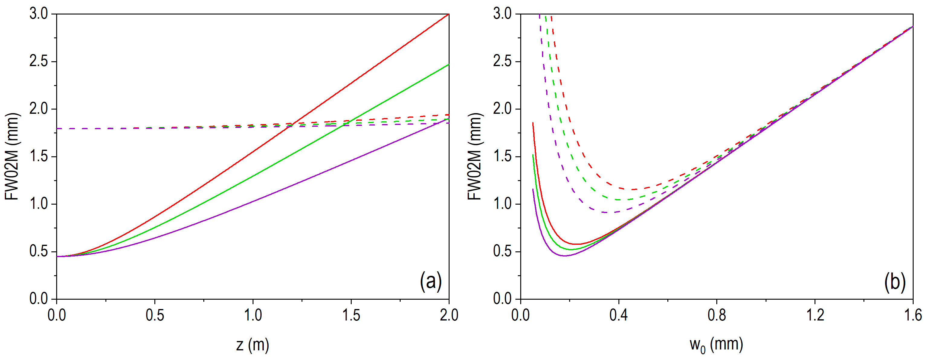
Figure 1: Full width at 20% the maximum intensity (FW02M) for a diffracted Gaussian beam in terms of its distance between the input and output planes (a) and the size of its waist (b) for three different values of the wavelength: $\lambda=650$ nm (red), $\lambda=532$ nm (green), and $\lambda=405$ nm (violet). To compare with, in panel (a) two input waist sizes are considered: $w_{0}=0.25$ mm (solid lines) and $w_{0}=1$ mm (dashed lines). Similarly, in panel (b) two input-output distances are considered: $z=0.25$ m (solid lines) and $z=1$ m (dashed lines).

e numerical representation of Eq. (11), describing the behavior of the FW02M, is displayed in Fig. 1. Although no experimental outcomes are reported here (all results shown arise from numerical calculations), realistic values have been chosen for the physical parameters involved, so that they can easily be reproduced even in a basic Optics laboratory. Thus, the three wavelengths considered correspond to values of standard laser pointers, $\lambda=650$ nm, $\lambda=532$ nm, and $\lambda=405$ nm, with maximum output power below 5 mW and uncertainties of the order of $\pm 10$ nm, but that basically cover the visible spectral range. The FW02M dependence on the distance between the input and output planes, $z$, as given by Eq. (11), is shown in Fig. 1(a) for two values of the input waist, $w_{0}=0.25$ mm (solid lines) and $w_{0}=1$ mm (dashed lines), and the above three wavelengths (each curve with the corresponding color: red, green, and violet). As it can be noticed, the wider the Gaussian beam at the input plane the lesser its spreading at the output plane, which implies an also lesser difference among the results for the three wavelengths. Furthermore, it is also clearly seen that, as the beam size decreases, its three characteristic regimes, Huygens, Fresnel, and Fraunhofer, are more clearly distinguishable. For instance, for $w_{0}=0.25$ mm, the FW02M remains basically constant up to $z\approx 0.05$ m, then it undergoes a nearly quadratic (hyperbolic) increase up to $z\approx 0.3$ m, and finally it exhibits a linear increase regardless of the value of $z$. For the wider beam, though, with $w_{0}=1$ mm, the linear regime is not reached within the range of 2 m here considered, but we can only observe the nearly constant width characterizing the Huygens regime for the three wavelengths. Note that, if we consider an average wavelength $\bar{\lambda}=529$ nm, the Rayleigh range corresponding to $w_{0}=0.25$ mm is $\bar{z}_{R}=0.37$ m, while for $w_{0}=1$ m we have $\bar{z}_{R}=5.94$ m, both is agreement with the values inferred from the numerical results. Yet, the gradual increase observed with $z$ does not allow us to set a clear distinction between the Fraunhofer regime and the geometrical optics one. The same happens if, instead of varying $z$, we had chosen to vary $\lambda$, according to Eq. (11).

In order to make apparent the transition from the Fraunhofer regime to a seemingly geometrical optics regime, let us now analyze the dependence of Eq. (11) on the value of the input waist $w_{0}$. The numerical representation of Eq. (11) is shown in Fig. 1(b) for the same three wavelengths (same color code) and two different distances between the input and output planes, $z$: $z=0.25$ m (solid lines) and $z=1$ m (dashed lines). The picture that emerges this time is quite different, with two well-defined trends for the two distances and all wavelengths, one of them falling down with $w_{0}$, in agreement with Eq. (12), and another one exhibiting a linear increase with $w_{0}$, as described by Eq. (13). Furthermore, it is also clearly seen how an increase in the wavelength or in the distance to the output plane produce an increase in the position of the transition input waist, $w_{c}$, in agreement with the fact that decreasing any of these quantities (or both) enhances the wave (Fraunhofer diffraction) behavior of the beam, i.e., the FW02M will increase very quickly as a consequence of the fast dispersion of the beam at the Fraunhofer regime. On the contrary, this also implies that, to observe features typical of a geometrical optics regime, the width of the input beam should be pretty larger. Nonetheless, interestingly, in this latter case, in agreement with Eq. (13), the FW02M becomes asymptotically independent of the wavelength $\lambda$ or the input-output distance $z$, which is the distinctive trait of a typically geometrical optics regime. These simple numerical examples thus show us how the same field (a Gaussian beam, in this case) can transition from a behavior typical of the wave optics to another characteristic of the geometrical optics by only gradually changing a single parameter. Furthermore, while in the latter regime the behavior is invariant with the wavelength or the observation distance, in agreement with the outcomes extracted from the traditional scalar theory of diffraction, in the fully wave (Fraunhofer) regime there is a clear dependence on those parameters, making the FW02M highly sensitive to small variations of them. This is clearly seen as $w_{0}$ decreases, getting closer to the critical value determining the transition threshold. Note that this critical value undergoes a displacement towards larger values of the input waist as either $\lambda$ or $z$ (or both) increase. For instance, with the values here considered, for the same wavelength, this displacement doubles when the projection screen is moved from $z=0.25$ m to $z=1$ m.

Before concluding this section, we would like to briefly mention that the general shape displayed by the graphs in Fig. 1(b), and particularly the presence of a turnover that separates two physically different trends or behaviors, to some extent resembles a result found in quantum gravity, for micro-black holes, in the context of the so-called generalized uncertainty principle [11]. Within this scenario, the quantity that plays the role of the critical beam width $w_{0}$ is the Planck energy, observing a similar trend between a given space region of a certain width and the energy that it contains. If quantum fluctuations are important, then there is an inverse relation between the two quantities; if classical gravitation is relevant, then they are proportional. The critical length at which these two behaviors coincide is precisely the Planck length (for energy uncertainties of the order of the Planck energy), at which a micro black hole could originate.

3 Diffraction by a long rectangular slit

3.1 Theoretical analysis

Let us now consider the diffraction through a very long rectangular slit, with the $x$-axis in the direction of the shorter opening, with a width $a$, and the $y$-axis along the longer one, with a width $b\gg a$. Due to translation symmetry along the $y$-direction, the problem can be solved and explained, in a good approximation, within the $XZ$-plane, where $x$ will denote the transverse coordinate and $z$ the longitudinal (propagation) one. Appealing again to paraxial conditions, the electric field amplitude, solution of the (paraxial) Helmholtz equation, can be recast [1] as

$$E(x,z)\propto E_{0}\int_{-a/2}^{a/2}e^{i\pi(x-x^{\prime})^{2}/\lambda z}dx^{\prime},$$ (16)

in the case of an incident field with constant amplitude within the opening determined by the slit, from $-a/2$ to $a/2$, and where prefactors and global phase factors are neglected for simplicity, but without any loss of generality (a detailed derivation of the general paraxial solution can be found in [12] in the context of matter waves and the Schrödinger equation). If the output plane $z$ is fixed, Eq. (16) can be rewritten as

$$E(x,z)\propto E_{0}\int_{-a/2}^{a/2}e^{i(x-x^{\prime})^{2}/w_{c}^{2}}dx^{\prime},$$ (17)

where $w_{c}$ coincides with the value given by Eq. (14). Nonetheless, note that this parameter now describes a general distance that can be used to compare with, i.e., it is not the waist of a Gaussian beam.

As in Sec. 2, here we also consider the relative intensity distribution,

$$I_{\rm rel}(x,z)=\frac{I^{2}(x,z)}{I^{2}(0,z)}\propto\left|\int_{-a/2}^{a/2}e^{i(x-x^{\prime})^{2}/w_{c}^{2}}dx^{\prime}\right|^{2},$$ (18)

where $I(x,z)\propto|E(x,z)|^{2}$, $x^{\prime}$ and $x$ describe positions on the input and output plane, respectively (which correspond to the planes where the slit and the projection screen are accommodated). In principle, the next step in the analysis would consist, also as in Sec. 2, in investigating the behavior of (18) and determining the different propagation regimes. However, this task is not analytical for intermediate stages at the Fresnel regime, which requires the use of numerical techniques. Yet, the integral is simple enough to allow us extracting some physical insight leaving aside further calculations (even though they are eventually necessary to determine and understand the full trend). Thus, consider the integral

$$\mathcal{I}(x,z)=\int_{-a/2}^{a/2}e^{i({x^{\prime}}^{2}-2xx^{\prime})/w_{c}^{2}}dx^{\prime},$$ (19)

where the factor $e^{ix^{2}/w_{c}^{2}}$ is disregarded, because it is eventually suppressed in (18), and hence it has no physical relevance at all here. In order to make apparent the three regimes described in Sec. 2, the question to be addressed now is whether, for a given $z$ (or, in general, a given value of the typical length scale $w_{c}$), the phase factors ${x^{\prime}}^{2}$ and $2xx^{\prime}$ are relevant, and, in the affirmative case, which one of them is the leading one. When proceeding in this way, the following scenarios readily arise for a given wavelength of interest:

• If $z\approx 0$, the integrand becomes a very rapidly oscillatory function. On average, one could then assume that only when this function is evaluated over the actual point $x$ [i.e., $x^{\prime}\approx x$ in the integrand of Eq. (18)], there is a non-vanishing contribution to the integral; otherwise, it is rapidly vanishing. If this is extended to the full integration range, in a good approximation the result of the integral (19) is a constant, namely, $\mathcal{I}(x,z)\approx a$. This corresponds to a geometrical regime, where there is a nearly constant irradiance in front of the slit, surrounded on either side by a region of geometrical shadow. This thus corresponds to the Huygens regime, ruled out by geometrical optics, which holds for either small distances between input and output planes, but also, if $z$ is fixed, for negligible wavelengths.

• For longer but small enough values of $z$, so that the values $x$ of interest (where the intensity is important) are still within the $(-a/2,a/2)$ interval or nearby, the trend is similar, although the phase terms start playing a role, particularly, the ${x^{\prime}}^{2}$ term, which is typically smaller and hence leads to important oscillations. This quadratic dependence on the slit coordinate is typical of the Fresnel regime and physically manifests as the appearance of rather prominent oscillations in the intensity distribution, with some leaks towards the geometrical shadow region, even though it still mainly concentrates within the area covered by the slit. Note that, if the second phase term is neglected in Eq. (19), the Fresnel integrals readily appear, which leads to the usual methods in wave optics developed to determine analytically the on-axis intensity (Fresnel zones and the Cornu spiral).

• Finally, at rather long values of $z$ , far beyond the slit input plane, it is the second phase term the one that becomes prominent, since $x$ may acquire values beyond the interval $(-a/2,a/2)$. In this case, the integral (19) has a simple analytical solution:

  $$\mathcal{I}(x,z)\sim\int_{-a/2}^{a/2}e^{-2ixx^{\prime}/w_{c}^{2}}dx^{\prime}\propto{\rm sinc}\left(\frac{\pi ax}{\lambda z}\right).$$ (20)

  With this, the intensity (18) becomes

  $$I_{\rm rel}(x,z)={\rm sinc}^{2}\left(\frac{\pi ax}{\lambda z}\right),$$ (21)

  which is the typical intensity distribution generated by a single slit in the Fraunhofer regime. The profile displayed by this intensity distribution at the output plane, regardless of the value of $z$, only depends on the ratio $x/z$, which determines the observation angle, $\theta\approx x/z$, in paraxial approximation.

We thus see in a simple and intuitive manner that, effectively, the three regimes are a general trait of any diffraction process, independently of the shape of the initially diffracted field (the field at the input plane).

Let us know get back to the question of determining the width of the intensity distribution at a fixed output plane $z$, also measured in terms of the FW02M. From the above discussion, and following the reasoning given in [5], a suitable guess in the geometrical optics regime for the FW02M is

$${\rm FW02M}\propto a,$$ (22)

assuming that Fresnel diffraction features are negligible, at least, at first approximation. Of course, some deviations should be expected, but in the limit a very large slit width, the approximation should be good enough. On the contrary, for tiny slit widths, one should expect Fraunhofer diffraction to be dominant and a decreasing trend for FW02M with increasing $a$, as it is inferred from Eq. (21). In order to determine an analytical expression for the FW02M in this case, let us consider the sine approximation formula developed by the VIIth-century Indian astronomer and mathematician Bhaskara I [13],

$$\sin u\approx\frac{16u(\pi-u)}{5\pi^{2}-4u(\pi-u)},$$ (23)

where $u$ is measured in radians ($0\leq u\leq\pi$). From this formula, it follows that the sinc-function can be approximated as

$${\rm sinc}\ \!u\approx\frac{16(\pi-u)}{5\pi^{2}-4u(\pi-u)}.$$ (24)

Here, we have $u=\pi ax/\lambda z$. If we search for the value of $u$, such that ${\rm sinc}^{2}\ \!u=\beta^{2}$, we find

$$u=\frac{1}{2}\left(\pi-\frac{4}{\beta}+\frac{2}{\beta}\sqrt{4+2\pi\beta-\pi^{2}\beta^{2}}\right).$$ (25)

After substituting $\beta=\sqrt{0.2}=1/\sqrt{5}$ into this latter expression, we find

$$u=\frac{\pi}{2}-2\sqrt{5}+\sqrt{20-\pi^{2}+2\pi\sqrt{5}}\approx 2.01598$$ (26)

(the negative root is neglected, because of the domain of definition for $u$ indicated above). Therefore, the expression of the FW02M in the Fraunhofer regime reads as

$${\rm FW02M}\approx\frac{2u\lambda z}{\pi a}\approx 1.28341\ \frac{\lambda z}{a},$$ (27)

which shows the expected dependence on the inverse of the slit width $a$. Since there is not an analytical expression for the FW02M when the full range of slit widths is covered, as it happens with Gaussian slits, to determine in an approximate manner the critical width $a_{c}$ we assume that, for this value, Eqs. (22) and (27) must be equal. This renders a critical slit-width value

$$a_{c}\approx 1.13288\ \sqrt{\lambda z}\approx 2.00797\ \sqrt{\frac{\lambda z}{\pi}}.$$ (28)

If this value is substituted into Eq. (27), we obtain the approximated value for the turnover FW02M,

$${\rm FW02M}_{t}\approx 1.13287\ \sqrt{\lambda z}\approx 2.007966\ \sqrt{\frac{\lambda z}{\pi}},$$ (29)

which is about twice the turnover value found for the Gaussian beam.

Of course, the above conclusions are just reasonable analytical conjectures, which do not provide further details about the transition that we are studying here, and that must be validated in some way. Here, this will be done by numerically determining the FW02M. In particular, in order to get a deeper insight, next two intertwined routes are considered, namely, a numerical analysis, which renders some light on the trends analytically found (as it was done in the case of Gaussian slits), and then a (numerical) comparison with the experiment, with the purpose to verify the validity of such numerical analysis.

3.2 Numerical analysis

As in Sec. 2, in Fig. 2 we show the dependence of the FW02M on the distance between the input and output planes (a), and on the slit width $a$ (b), which is the analog to the Gaussian beam waist $w_{0}$. In each case, the same three wavelengths have been considered. More specifically, given the lack of analyticity of the FW02M along the full range of slit widths considered, it has to be numerically computed. Thus, to carry out the integral (19) that the intensity (18) is based on, a simple on-purpose Fortran code was programmed (based on the trapezoid rule, which suffices by far in this case), considering both a large box (in order to accommodate wide intensity distributions in both limits) and a large number of sampling points (to resolve the fastest oscillations in the Fresnel regime). Fixing the value of two parameters, the code automatically runs over a large set of values of the remaining parameter, thus rendering a smooth graph for the FW02M, analogous to the the graphs obtained from the analytical expressions for the Gaussian slit. In particular, the code computes the relative intensity distribution. (18), normalizes its maximum to unity, and then finds the $x$-positions ($x_{1}$ and $x_{2}$, symmetrically distributed around $x=0$) at which the latter equals 0.2 in order to determine the FW02M.

Proceeding in that way, we have thus obtained the results shown in Fig. 2(a) for two slit widths: $a=0.25$ mm (solid lines) and $a=1$ mm (dashed lines). Consider the case for the smallest slit width. Unlike the smooth dependence exhibited by the Gaussian beam, it is observed that there is a very short Huygens regime, followed by a saw-tooth structure characterizing the intermediate Fresnel regime; immediately afterwards, the Fraunhofer regime starts, which is clearly distinguished by its distinctive linear trend. If the slit width increases, the same behavior is observed, although the distance $z$ at which the Fraunhofer regime is reached increases very rapidly. Note that, on average, an increase from 0.25 mm to 1 mm in $a$ implies an increase from $\sim 0.05$ mm to $\sim 1$ mm. Although the near field structure is more complex than the same region for the Gaussian beam, we find again the same lack: it is difficult to observe the transition that we are investigating, because we cannot see a clear turnover.

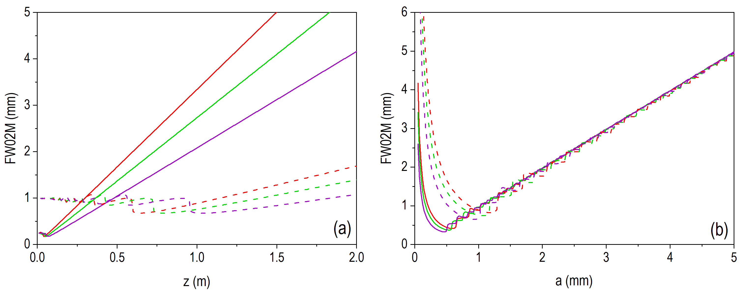
Figure 2: Full width at 20% the maximum intensity (FW02M) for the diffraction of a monochromatic plane waves incident on a very long rectangular slit in terms of the distance between the input and output planes $z$ (a) and the slit width $a$ (b) for three different values of the wavelength: $\lambda=650$ nm (red), $\lambda=532$ nm (green) and $\lambda=405$ nm (violet). To compare with, in panel (a) two slit widths are considered: $a=0.25$ mm (solid lines) and $a=1$ mm (dashed lines). Similarly, in panel (b) two distances are considered: $z=0.25$ m (solid lines) and $z=1$ m (dashed lines).

To overcome that problem, we proceed as before and compute the FW02M against the slit width, which is shown in Fig. 2(b) for the same three wavelengths and two values of the distance between the input and output planes: $z=0.25$ m (solid lines) and $z=1$ m (dashed lines). Thus, the numerical simulations render two important general trends. First, an initial falloff with increasing (but small values of) $a$, which is in compliance with the behavior described by Eq. (27), i.e., with the inverse of the slit width. Second, an incipient overall linear trend is observed for large values of $a$, which is in correspondence with the guess (22). Furthermore, we also find that there is a turnover denoted by the presence of a minimum in the representation, as in the case of the Gaussian beam [see Fig. 1(b)], which approximately coincides with the values estimated above for $a_{c}$ and ${\rm FW02M}_{t}$. For instance, if we consider the average wavelength $\bar{\lambda}=529$ nm, the turnover is obtained at $a_{c}\approx 0.4$ mm for $z=0.25$ m, and at $a_{c}\approx 0.8$ for $z=1$ m, which coincides with what we observe in Fig. 2(b). In either case, though, these values are larger than for a Gaussian beam, because the expansion of “top-hat” type diffracted beams is typically faster, which requires larger openings to observe slower diffractive rates. Nonetheless, it seems that the preliminary analytical treatment, based on a series of reasonable work hypotheses, is not that bad. However, what such an analytical treatment does not describe is the presence of the staircase structure that starts at the transition between the end of the Fraunhofer regime and the beginning of the Fresnel one, and somehow influences the turnover region, avoiding us to unambiguously identify a minimum (note that the minimum observable now is affected by such a staircase structure). Yet the extrapolation of a linear regression at large values of $a$, where the steps become smaller and smaller, allows us to determine the turnover from the intersection between this linear fitting and the Fraunhofer falloffs, which render basically the estimated values mentioned before.

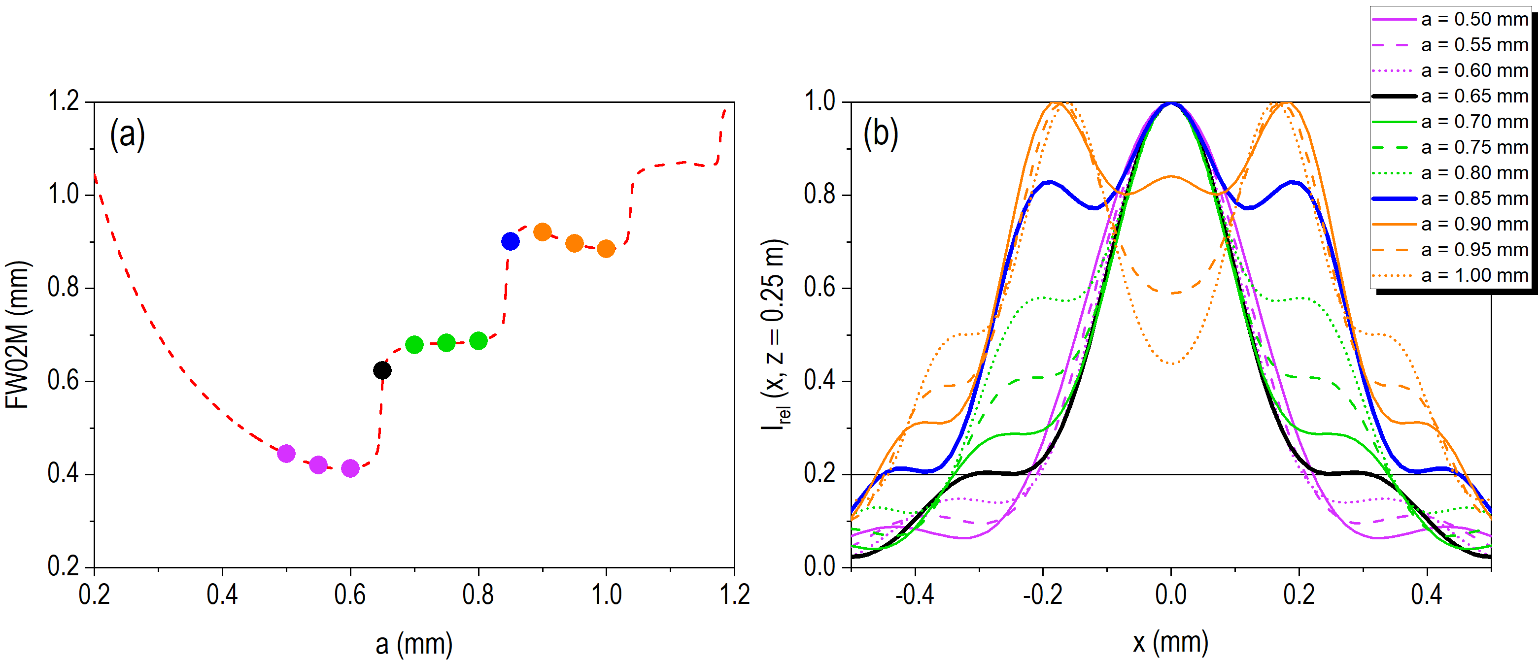
Figure 3: (a) Detail of the full width at 20% the maximum intensity (FW02M) displayed in Fig. 2 for $\lambda=650$ nm and $z=0.25$ m. Solid circles denote the sampling values considered to analyze the staircase structure displayed by the FW02M around the turnover region. (b) Relative intensity distributions (at $z=0.25$ m) associated with the selected values of slit widths shown in panel (a). Same color line (but different type) is used for values on the same step; thicker lines correspond to values at the jump.

The staircase structure of Fig. 2(b) is connected to the systematic method employed by our numerical code, which determines the precise value where the relative intensity reaches the 20% of its maximum value. In order to determine the origin of this distinctive structure, absent in the case of Gaussian beams, let us focus on an enlargement of Fig. 2(b) around the turnover region, displayed in Fig. 3(a). In the latter figure, the turnover region is seen for a wavelength $\lambda=650$ nm and a distance $z=0.25$ m. The numerical simulation is denoted with the black solid line. Some sampling values associated with different slit widths are also shown (red and blue solid circles), which cover three step levels and will be used to elucidate the origin of these steps (in particular, the blue circles are markers related to the border between one step and the next one). The relative intensities associated with each marker are shown in Fig. 3(b) with different colors, for slit widths ranging from 0.5 mm to 1 mm, in tiny increments of 0.05 mm. As it can be noticed, because the turnover region is fully immersed in the Fresnel regime (actually, for moderate values of $a$, we should talk about the intermediate regime between the Fraunhofer and Fresnel ones [3]), such small increments may induce important changes, as it is seen near the sudden jumps from one step to the next one. What happens is that the intensity is characterized by marginal oscillating “wings”, as seen in Fig. 3(b), which start developing as the Fraunhofer regime blurs, and diffraction minima no longer vanish, particularly those adjacent to the principal maximum. The general behavior of these minima is that they start increasing, progressively elevating with them the secondary maxima and generating a highly wavy intensity distribution as $a$ increases. Each time that one of these secondary maxima reaches the 20% intensity threshold, we observe a sudden increase in the corresponding FW02M. For example, in Fig. 3(b), this is seen to happen for $a=0.65$ mm (green thick solid line) and $a=0.85$ mm (black thick solid line); in the first case, the jump is associated with the disappearance of the first adjacent secondary maxima, while in the latter case the jump is connected to the second one. Note that, eventually, the intensity pattern displays the well-known profile of a nearly flat distribution, approximately along the same extension covered by the slit, modulated by a series of small-amplitude and rapidly-varying oscillations both at the top and also on the sides (in the regions of geometrical shadow). This is the typical behavior that is provided in Optics textbooks to illustrate the Fresnel regime [2, 1, 3], although, as seen in Fig. 2(b), it quickly approaches a nearly linear trend as $a$ increases well above $a_{c}$.

3.3 Comparison with the experiment

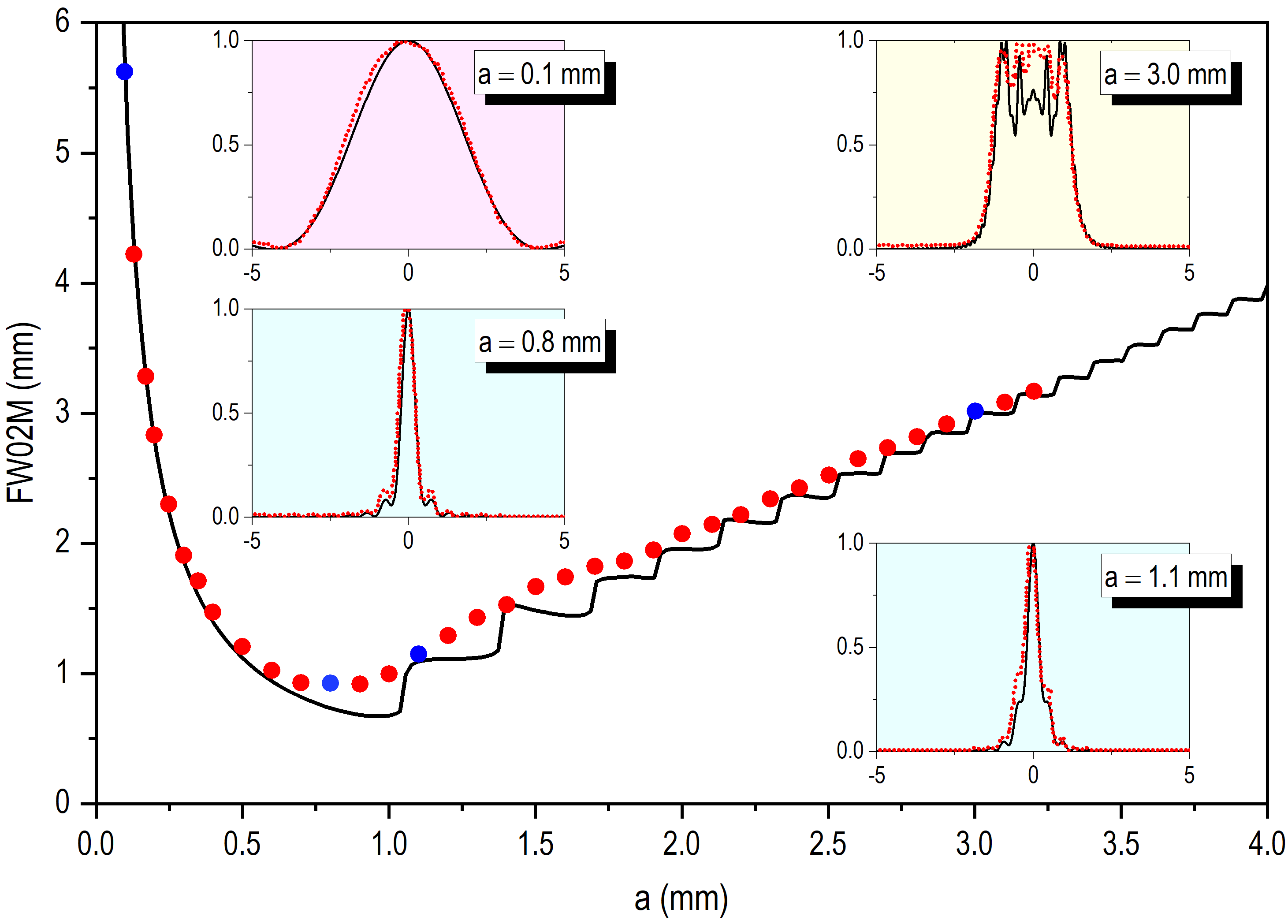
Figure 4: Comparison with the experimental data reported in [5], with $\lambda_{\rm exp}=660$ nm and $z_{\rm exp}=0.656$ m. In the main panel, the experimental data are denoted by solid circles, while the theoretical simulation following Eq. (18) is described by the black solid line. In the insets, relative intensity for four different values of the slit width $a$: $a=0.1$ mm, $a=0.8$ mm, $a=1.1$ mm, and $a=3.0$ mm. Again here the red solid circles refer to experimental data, while the solid line indicates the intensity rendered by the theoretical model, Eq. (18). These four particular cases are denoted in the main panel with blue solid circles and have been picked up in different regimes, two in the limiting cases (Fraunhofer and geometrical optics regimes) and two in the turnover region.

In order to test the validity of the approach that we have followed here, let us now compare with the experimental data reported in [5]. An alternative theoretical analysis has been previously reported in [6] considering the variation of the intensity distribution in terms of the Fresnel number (zones), $FN=a^{2}/4\lambda z$. In Fig. 4 we show the numerically computed FW02M as a function of the slit width, which has been obtained by using the same raw values for $\lambda$ and $z$ considered in the experiment reported in [5], namely $\lambda_{\rm exp}=660$ nm and $z_{\rm exp}=0.656$ m, without any extra fitting and/or numerical treatment. As it is seen, the theoretical (numerical) representation exhibits the typical staircase structure beyond the turnover region above described, which gradually approaches a nearly linear tail for large $a$. Comparing the experimental data (solid circles), directly extracted from [5] and inserted in the representation (also without any extra treatment), with the theoretical (numerical) results, it is found that there is a good agreement, in particular, concerning the overall trend. The staircase structure, though, is not observed in the experiment. After closely inspecting and analyzing the experimental data, particularly observing the slight discrepancies between the theoretical and experimental intensity distributions (some of which are represented in the insets for the slit widths indicated), we come to the conclusion that, in order to observe the staircase structure, the quality of the data recording procedure requires some further refinement, for small fluctuations around the sudden jumps will suppress the effect. Nonetheless, getting back to the experimental data shown in Fig. 4, we find that the turnover region is around the critical value that we directly obtain from Eq. (28) for $\lambda_{\rm exp}$ and $z_{\rm exp}$, namely, $a_{c}\approx 0.74$ mm, which is closer to the experimental turnover than the former estimate, $a_{c}\approx 0.931$ mm, provided in [5].

4 Final remarks

In this work, an analysis of the transition from the Fraunhofer diffraction regime to the geometrical optics limit has been carried out with the purpose to better understand the meeting point between wave optics and geometrical optics, and hence to get a deeper insight into the physical origin and consequences of the latter, alternative to wavelength-based considerations. Motivated by the experiments carried out by Panuski and Mungan [5], which show how this transition takes place in a nice manner, beyond such wavelength-based considerations, here we have tackled the issue by first investigating the behavior of Gaussian beams and then the case of single slit diffraction. In both cases it has been observed how, by means of analytical treatments, whenever the width of the intensity profile is analyzed in terms of the effective slit width (the beam waist or the actual slit width), a turnover critical value for this width readily arises, which depends on two parameters, namely, the wavelength $\lambda$ of the monochromatic source considered, and the distance $z$ between the input (slit) and output (projection screen) planes. Analytical expressions have been found for the critical values in the two cases considered, both being proportional to $\sqrt{\lambda z}$. Accordingly, it is seen that the rapid falloff with the inverse of the slit width, which characterizes the width of the intensity distribution in the Fraunhofer regime, gives rise to a linearly increasing width of such a distribution beyond the critical value, in correspondence with the expectations from a geometrical optics point of view.

Theoretical (numerical) results have also been compared to experimental data extracted from [5], finding a good agreement and, in particular, a systematic way to determine the value of the turnover condition from a theoretical model. Actually, the numerical results have shown evidence that, while the Fraunhofer falloff is clearly seen, the transition towards the geometrical regime goes through a staircase structure with shorter and shorter steps, starting within the turnover region. This structure is directly related to the gradual suppression of the typical Fraunhofer diffraction pattern, where each step in the staircase corresponds to a sort of quantized increase of the FW02M coming from the adjacent secondary maxima. Although the experimental data reported in [5] do not allow to observe this structure, they fit pretty well the asymptotic behavior towards the geometrical regime.

To conclude, it is worth mentioning that the treatments and findings account for here can be straightforwardly extended to matter waves. As it was mentioned above, in Sec. 2, the isomorphism between the paraxial Helmholtz equation and the time-dependent Schrödinger equation enables a direct translation of the findings reported here to matter waves, which, in principle, should be observable with the appropriate experimental conditions. Since fundamental aspects of interference have been explored with electrons [14, 15] and large molecular complexes [16, 17, 18], these systems could also be used to investigate the behaviors here observed. Another interesting extension of the present study is that of the so-called fractional Schrödinger equation [19, 20, 21], which also applies to both massive quantum particles and light (where it is used in the form of a fractional paraxial Helmholtz equation), and is governed by a fractional spatial derivative. In this latter regard, the action of a fractional Laplacian over the diffracted beam is expected to render novel limits in both the Fraunhofer diffraction regime and the geometrical optics one.

References

References

- [1] Born M and Wolf E 1999 Principles of Optics. Electromagnetic Theory of Propagation, Interference and Diffraction of Light 7th ed (Cambridge: Cambridge University Press)
- [2] Hecht E 2002 Optics 4th ed (New York: Addison-Wesley Longman)
- [3] Elmore W C and Heald M A 1969 Physics of Waves (New York: McGraw-Hill)
- [4] F S Harris J, Tavenner M S and Mitchell R L 1969 J. Opt. Soc. Am. 59 293–296
- [5] Panuski C L and Mungan C E 2016 Phys. Teacher 54 356–359
- [6] Davidović M D and Božić M 2019 Phys. Teacher 57 176–178
- [7] Sanz A S and Miret-Artés S 2012 A Trajectory Description of Quantum Processes. I. Fundamentals (Lecture Notes in Physics vol 850) (Berlin: Springer)
- [8] Sanz A S, Davidović M and Božić M 2020 Appl. Sci. 10 1808(1–25)
- [9] Sanz A S and Miret-Artés S 2012 Am. J. Phys. 80 525–533
- [10] Sanz A S 2012 J. Phys.: Conf. Ser. 361 012016(1–11)
- [11] Scardigli F 199 Phys. Lett. B 452 39–44
- [12] Sanz A S, Davidović M and Božić M 2015 Ann. Phys. 353 205–221
- [13] Shirali S A 2011 Math. Mag. 84 98–107
- [14] Bach R, Pope D, Liou S H and Batelaan H 2013 New J. Phys. 15 033018(1–7)
- [15] Beierle P J, Zhang L and Batelaan H 2018 New J. Phys. 20 113030(1–12)
- [16] Arndt M, Nairz O, Vos-Andreae J, Keller C, van der Zouw G and Zeilinger A 1999 Nature 401 680–682
- [17] Gerlich S, Eibenberger S, Tomandl M, Nimmrichter S, Hornberger K, Fagan P J, Tüxen J, Mayor M and Arndt M 2011 Nat. Commun. 2:263 1–5
- [18] Juffmann T, Milic A, Müllneritsch M, Asenbaum P, Tsukernik A, Tüxen J, Mayor M, Cheshnovsky O and Arndt M 2012 Nat. Nanotech. 7 297–300
- [19] Longhi S 2015 Opt. Lett. 40 1117–1120
- [20] Zhang Y, Liu X, Belić M R, Zhong W, Zhang Y and Xiao M 2015 Phys. Rev. Lett. 115 180403(1–5)
- [21] Zhang Y, Zhong H, Belić M R, Zhu Y, Zhong W, Zhang Y, Christodoulides D N and Xiao M 2016 Laser Photonics Rev. 10 526-531