Technical Report: A Totally Asynchronous Algorithm for Tracking Solutions to Time-Varying Convex Optimization Problems

Abstract

This paper presents a decentralized algorithm for a team of agents to track time-varying fixed points that are the solutions to time-varying convex optimization problems. The algorithm is first-order, and it allows for total asynchrony in the communications and computations of all agents, i.e., all such operations can occur with arbitrary timing and arbitrary (finite) delays. Convergence rates are computed in terms of the communications and computations that agents execute, without specifying when they must occur. These rates apply to convergence to the minimum of each individual objective function, as well as agents’ long-run behavior as their objective functions change. Then, to improve the usage of limited communication and computation resources, we optimize the timing of agents’ operations relative to changes in their objective functions to minimize total fixed point tracking error over time. Simulation results are presented to illustrate these developments in practice and empirically assess their robustness to uncertainties in agents’ update laws.

I Introduction

Time-varying convex optimization problems arise in machine learning, signal processing, robotics, power systems, and others [1, 2, 3, 4, 5]. Such problems can model, for example, time-varying demands in power systems [6], and uncertain, dynamic environments for real-time control of autonomous vehicles [7]. Often, these problems are solved with networks of agents, e.g., the robots that are given a time-varying task specification or a network of processors across which computations have been parallelized. Such instances then require a multi-agent algorithm to solve time-varying problems.

Many multi-agent systems face asynchrony in agents’ communications and computations. For example, asynchronous communications can result from environmental hazards that impede communications and/or interference among communication signals. Asynchronous computations onboard agents can result from clock mismatches and different computational hardware. As a result, agents may generate and share information with unpredictable timing. Asynchrony has been studied for static optimization problems in numerous ways, e.g., [8, 9, 10, 11, 12]. In particular, [13] establishes conditions for the convergence of static optimization under total asynchrony, namely communications and computations with arbitrary delays. To the best of our knowledge, total asynchrony remains unaddressed in time-varying optimization, and this paper fills this gap.

The algorithm we present uses totally asynchronous gradient descent to track time-varying fixed points that are the solutions to time-varying convex optimization problems. It is block-based, in the sense that each agent updates and communicates only a small subset of the decision variables in a problem. Due to total asynchrony, these operations can occur with arbitrary timing, which precludes the development of convergence rates that depend on delay bound parameters [14, 15, 16, 17]. In this work, convergence rates are instead derived that depend upon how agents’ communications and computations are interleaved over time. These results enable the quantification of the quality of agents’ fixed point tracking in terms of what they execute, without specifying when operations must occur.

While it may be difficult to control the exact timing of all agents’ operations, it is easier for individual agents to control the sequence of their own local operations (without needing to control their exact timing). To leverage this capability, the aforementioned convergence rates are used to optimize the sequence of agents’ operations. This is done by optimizing (in a way made precise in Section V) the order of communications and computations, both relative to each other and relative to the timing of changes in objective functions. Specifically, a constrained optimization problem is formulated and solved in closed form to minimize agents’ convergence rates (through their dependence on agents’ operations) under constraints on communicating and computing.

Summary of Contributions: In summary, the contributions of this paper are:

• We show that the totally asynchronous gradient descent algorithm can track solutions to time-varying convex optimization problems (Section IV).

• We derive tracking bounds of the proposed algorithm in both the asymptotic and finite-time cases. These bounds quantify the dependence of agents’ performance upon their communications and computations, as well as problem parameters (Theorem 2 and Corollary 1).

• For problems in which agents can execute a limited number of computations and communications, we optimize the sequence of agents’ operations to achieve desired tracking error. Namely, a constrained optimization problem is solved in closed form to determine the optimal sequence of communications and computations to enforce a desired bound on fixed point tracking error (Theorems 3 and 4 and Corollary 2).

• We empirically demonstrate the robustness to noise of the totally asynchronous gradient descent algorithm in a time-varying problem (Section VI).

Related Work There is a large corpus of research on multi-agent optimization, and we cite only a few representative examples. Asynchronous block-based algorithms include seminal work in [18, 13, 19] and recent developments in [20, 21, 22, 23, 24], which all consider static optimization problems. We differ by studying time-varying problems.

This paper is also closely related to a growing body of research on feedback optimization, which often includes time-varying optimization problems. Relevant work develops prediction-correction algorithms for problems with time-varying objective functions in both the centralized [25, 26] and distributed cases [27, 28]. Specifically, [27] considers an objective function that is the sum of locally available functions at each node and uses higher-order information to perform the prediction step. The present work considers objective functions of an arbitrary form and requires only first-order information. Moreover, the objective functions we consider change discretely in time and they need not be sampled from an objective function that varies continuously in time. Changes in the objective function thus cannot be predicted reliably, and we do not use a prediction step.

In [27, Section 1], it is noted that correction-only algorithms (which we consider) cannot effectively mitigate tracking error of the optimizer if the optimization problem and algorithm do not have sufficient timescale separation. In this work, some timescale separation is indeed required, in the sense that objective functions must not vary in time faster than agents can perform computations and communications (Section III provides a detailed discussion). We note that the need for timescale separation is motivated by feasibility rather than technical convenience: if objectives can change faster than agents can compute and communicate, then agents will be unable to track time-varying fixed points and we cannot hope to prove anything useful.

In [28, Remark 3], it is noted that distributed time-varying optimization by agents with different computational abilities is subject to ongoing research. To the best of our knowledge, this problem remains open, and we present a solution to it by allowing agents to both compute and communicate totally asynchronously.

The rest of the paper is organized as follows. Section II states the problems of interest. Section III states the algorithm for solving them. Then, Section IV develops convergence rates for agents’ short-term and asymptotic behavior. Section V optimizes agents’ communications and computations to improve tracking over time. After that, Section VI provides simulation results, and Section VII concludes.

II Problem Formulation

This section gives a formal problem statement and the assumptions placed on it. Throughout, this paper solves problems with a network of $N$ agents indexed over the set $[N]:=\{1,\ldots,N\}$. We consider problems of the following form over a time horizon $\mathcal{T}=\{0,\ldots,T\}$ for $T\in\mathbb{N}$.

Problem 1.

With $N$ agents, over a time horizon $\mathcal{T}$,

$$\begin{split}\underset{u}{\textnormal{minimize}}&\ f(u,t)\\ \textnormal{subject to}&\ u\in U,\end{split}$$ (1)

where $U\subseteq\mathbb{R}^{n}$, $f:\mathbb{R}^{n}\times\mathbb{N}\rightarrow\mathbb{R}$, and $t\in\mathcal{T}$ is time.

We make the following assumptions about Problem 1.

Assumption 1.

For all $t\in\mathcal{T}$, the function $f(\cdot,t)$ is twice continuously differentiable.

Assumption 1 guarantees the existence and continuity of both the gradient and the Hessian of $f(\cdot,t)$. Many functions satisfy this assumption, such as polynomials of all orders.

Assumption 2.

The constraint set $U$ can be decomposed via

$$U=U_{1}\times U_{2}\times\cdots\times U_{N},$$ (2)

where $U_{i}\subseteq\mathbb{R}^{n_{i}}$, $n_{i}\in\mathbb{N}$, is non-empty, compact, and convex.

Assumption 2 permits constraints such as box constraints, and it implies that $U$ is also non-empty, compact, and convex. It also ensures that each agent can update its block of decision variables independently, which will be used to develop a distributed gradient projection law for enforcing the set constraint $u\in U$. Similarly, $u\in U$ can be decomposed via

$$u=\left(\begin{array}[]{c}u_{1}\\ \vdots\\ u_{N}\end{array}\right),$$ (3)

where $u_{i}\in U_{i}\subseteq\mathbb{R}^{n_{i}}$. We define

$$p_{u}=[n_{1},n_{2},\ldots,n_{N}]\in\mathbb{N}^{N}$$ (4)

to be the vector of dimensions of the blocks into which $u$ is partitioned. From Assumptions 1-2, we have that ${H(\cdot,t)\coloneqq\nabla^{2}f(\cdot,t)}$ is continuous and $U$ is compact. Therefore, ${\nabla f}(\cdot,t)$ is Lipschitz continuous. For each $t\in\mathcal{T}$, we use $L_{t}$ to denote the bound on ${\|H(\cdot,t)\|_{2}}$ over $U$, and this $L_{t}$ is the Lipschitz constant of ${\nabla f}(\cdot,t)$ over $U$.

The next assumption uses strict block diagonal dominance of partitioned matrices. Suppose a matrix $A\in\mathbb{R}^{n\times n}$ is partitioned into blocks according to the partition vector ${p_{u}=[n_{1},\ldots,n_{N}]}$, where $\sum_{i=1}^{N}n_{i}=n$ (we allow $n_{i}\neq n_{j}$ for all $i\neq j$). Let $\left[A\right]_{p_{u}}$ denote the partitioned matrix, i.e.,

$$\left[A\right]_{p_{u}}=\begin{bmatrix}A_{11}&A_{12}&\cdots&A_{1N}\\ A_{21}&A_{22}&\cdots&A_{2N}\\ \vdots&\vdots&\ddots&\vdots\\ A_{N1}&A_{N2}&\cdots&A_{NN}\end{bmatrix}.$$ (5)

The $i^{th}j^{th}$ block, denoted $A_{ij}\in\mathbb{R}^{n_{i}\times n_{j}}$, is the matrix block of the rows of $[A]_{p_{u}}$ with indices $\sum_{k=1}^{i-1}n_{k}+1$ through $\sum_{k=1}^{i}n_{k}$ and the columns of $[A]_{p_{u}}$ with indices $\sum_{k=1}^{j-1}n_{k}+1$ through $\sum_{k=1}^{j}n_{k}$, i.e., $A_{11}$ is the first $n_{1}$ columns of the first $n_{1}$ rows, $A_{12}$ is the next $n_{2}$ columns of the first $n_{1}$ rows, etc.

Assumption 3.

The matrix $H(u,t)$ can be partitioned with respect to $p_{u}$ from Equation (4), and $H_{ii}(u,t)$ is symmetric and positive definite for all $u\in U$ and each $t\in\mathcal{T}$, i.e., $H_{ii}(u,t)=H_{ii}(u,t)^{T}\succ 0$. Moreover, for each $t\in\mathcal{T}$, $H(u,t)$ is $\beta_{t}$-strictly block diagonally dominant, i.e., for some $\beta_{t}>0$

$$\left(\left\|H_{ii}(u,t)^{-1}\right\|_{2}\right)^{-1}\geq\underset{j\neq i}{\sum_{j=1}^{n}}\left\|H_{ij}(u,t)\right\|_{2}+\beta_{t}.$$ (6)

As noted in [13, Section 6.3.2], Assumption 3 is sufficient to ensure that agents’ iterates contract towards the minimizer of $f(\cdot,t)$ (in an appropriate norm) for fixed $t$. And, in a way made precise in [13, Section 6.3.1], a problem is unlikely to be solvable by a totally asynchronous algorithm if it fails to satisfy Assumption 3. Thus, we enforce it here. One consequence of Assumption 3 is given next.

Lemma 1.

Let Assumptions 1-3 hold. Then $f(\cdot,t)$ is $\beta_{t}$-strongly convex and it has a unique minimizer, denoted $\hat{u}^{t}$.

Proof: From [21, Lemma 4], it immediately follows that

$$\lambda_{min}\big{[}H(u,t)\big{]}\geq\big{(}\|H_{ii}(u,t)^{-1}\|_{2}\big{)}^{-1}-\underset{j\neq i}{\sum_{j=1}^{n}}\left\|H_{ij}(u,t)\right\|_{2}$$ (7)

for all $u\in U$ and $t\in\mathcal{T}$. Therefore by Assumption 3,

$$\lambda_{min}\big{[}H(u,t)\big{]}\geq\beta_{t}$$ (8)

for all $u\in U$ and $t\in\mathcal{T}$. This implies that $f(\cdot,t)$ is $\beta_{t}$-strongly convex [29, Section 9.1.2], from which the uniqueness of the minimum $\hat{u}^{t}\coloneqq\underset{u\in U}{\text{argmin}}\ f(u,t)$ follows. $\blacksquare$

Regarding changes over time, the following is assumed.

Assumption 4.

For each $t\in\mathcal{T}$, there exists a constant ${\sigma_{t}\geq 0}$ such that $\left\|\hat{u}^{t+1}-\hat{u}^{t}\right\|_{2}\leq\sigma_{t}$.

Without Assumption 4, a problem could change by arbitrarily large amounts, and it would not be possible to track the solution of Problem 1.

III Asynchronous Update Law

In this section we develop the totally asynchronous algorithm for tracking time-varying fixed points. First, we describe the relationship between the times at which the objective function changes and the times at which agents execute communications and computations.

III-A Time and Timescale Separation

Problem 1 evolves over time, indexed by the discrete time index $t$, and, in defining agents’ algorithm, we will index their operations over the discrete time index $k$. The reason is that the timing of agents’ computations and communications need not coincide with changes in their objective functions. For example, agents may execute several communications and computations when minimizing $f(\cdot,t)$ for each $t\in\mathcal{T}$. If this were not done, then the problem could evolve faster than agents compute and communicate, and tracking a time-varying fixed point would be infeasible. Thus, it is necessary to adopt a formalism that enables agents to perform multiple operations to minimize $f(\cdot,t)$ for each $t\in\mathcal{T}$.

In particular, we require some timescale separation between the ticks of $t$, the time index for changes in the objective function, and the ticks of $k$, the index of agents’ operations. For for each $t\in\mathcal{T}$, some number of ticks $\kappa_{t}\geq 1$ of $k$ elapse before $t$ increments to $t+1$. Agents may compute and/or communicate something at each tick of $k$, though this is not guaranteed due to asynchrony. In other words, timescale separation allows for the possibility that agents perform multiple communications and computations for each $t$, though we by no means assume that they do so. As will be shown below, our analysis allows for (and quantifies the effects of) scenarios in which agents perform no operations at all. Of course, timescale separation is not new to this work, and has been used, e.g., in optimization and model predictive control in [30, 31, 32].

III-B Formal Algorithm Statement

We consider a block-based gradient algorithm with totally asynchronous computations and communications to solve Problem 1 over a network of $N$ agents. Each agent updates only a subset of the entire decision vector and communicates the values of their sub-vector with the rest of the network over time. Asynchrony implies that agents receive different information at different times, and thus we expect them to have differing values for decision variables onboard. At any time $k$, agent $i\in\left[N\right]$ has a local copy of its decision vector, denoted $u^{i}(k)\in\mathbb{R}^{n}$. Due to computation and communication delays, we allow $u^{i}(k)\neq u^{j}(k)$ for $j\neq i$. Within the vector $u^{i}(k)$, agent $i$ computes updates only to $u_{i}^{i}(k)\in\mathbb{R}^{n_{i}}$. At any time $k$, agent $i$ has (possibly old) values for agent $j$’s sub-vector of the decision variables, denoted $u_{j}^{i}(k)\in\mathbb{R}^{n_{j}}$. These are updated only by agent $j$ and then shared with the rest of the network.

At time $k$, if agent $i$ computes an update to $u^{i}_{i}(k)$, its computations are in terms of the decision vector $u^{i}(k)$. The entries of $u_{j}^{i}(k)$ for $j\neq i$ are obtained by communications from agent $j$, which may be subject to delays. Therefore, agent $i$ may (and often will) compute updates to $u^{i}_{i}$ based on outdated information from other agents.

Let $K^{i}$ be the set of times at which agent $i$ computes an update to $u^{i}_{i}$. Similarly, let $C^{i}_{j}$ be the set of times at which agent $j$ receives a transmission of $u^{i}_{i}$ from agent $i$; due to communication delays, these transmissions can be received at any time after they are sent, and they can be received at different times by different agents. We emphasize that the sets $K^{i}$ and $C^{i}_{j}$ are only defined to simplify discussion and analysis. Agents do not know and do not need to know $K^{i}$ and $C^{i}_{j}$. We define $\tau_{j}^{i}(k)$ to be the time at which agent $j$ originally computed the value of $u^{i}_{j}$ that agent $i$ has onboard at time $k$; agents $i$ and $j$ also do not need to know $\tau^{i}_{j}$. Formally,

$$u^{i}_{j}(k)=u^{j}_{j}\big{(}\tau^{i}_{j}(k)\big{)}.$$ (9)

Then $k-\tau_{j}^{i}(k)$ is the length of communication delay, and we emphasize that we do not assume any bound on agents’ delays. Instead, only the following is enforced.

Assumption 5.

For all $i\in[N]$, the set $K^{i}$ is infinite. Let $\{k_{d}\}_{d\in\mathbb{N}}$ be a non-decreasing sequence in $K^{i}$ tending to infinity. Then for all $i\in[N]$ and $j\in[N]\backslash\{i\}$, we have

$$\lim_{d\to\infty}\tau^{i}_{j}(k_{d})=\infty.$$ (10)

And messages are received in the order they were sent.

Assumption 5 ensures that (i) no agent ever stops computing updates (because $K^{i}$ is infinite), (ii) no agent ever stops sharing its updates with other agents (because $\tau^{i}_{j}(k_{d})$ tends to infinity), and (iii) arbitrarily old information cannot be received arbitrarily late into the run of an algorithm. This assumption is one of feasibility: there is no tracking of fixed points (and nothing to prove) if any agent ever permanently stops computing and/or communicating, or if arbitrarily old information can be received at any time.

We propose to use a gradient-based update law for agent $i$, which takes the form

$$u_{i}^{i}(k+1) =\begin{cases}\Pi_{U_{i}}\!\left[u_{i}^{i}(k)\!-\!\gamma_{t}\left(\nabla_{u_{i}}f(u^{i}(k),t)\right)\right]&k\!\in\!K^{i}\\ u_{i}^{i}(k)&k\!\notin\!K^{i}\end{cases}$$ (11)

$$u_{j}^{i}(k+1) =\begin{cases}u_{j}^{j}(\tau_{j}^{i}(k))&k\in C^{j}_{i}\\ u_{j}^{i}(k)&k\notin C^{j}_{i}\end{cases},$$ (12)

where $\gamma_{t}>0$ is the stepsize used when minimizing $f(\cdot,t)$. Bounds on $\gamma_{t}$ are established later in Proposition 1. Algorithm 1 provides pseudocode for agents’ updates; for notational convenience, we set $\kappa_{-1}=0$.

Input: $u_{j}^{i}(0)$ for all $i,j\in[N]$, $T\in\mathbb{N}$

1

2$k_{loop,-1}=-1$

3for t=0:T do

4       $k_{loop,t}=k_{loop,t-1}+\kappa_{t-1}$

5      for $k=k_{loop,t}+1:k_{loop,t}+\kappa_{t}$ do

6             for i=1:N do

7                   for j=1:N do

8                         if $k\in C^{j}_{i}$ then

9                                $u_{j}^{i}(k+1)=u_{j}^{j}(\tau^{i}_{j}(k))$

10                         end if

11                        else

12                                $u_{j}^{i}(k+1)=u_{j}^{i}(k)$

13                         end if

14                        

15                   end for

16                  if k $\in K^{i}$  then

17                         ​​​${u_{i}^{i}(k\!+\!1)\!=\!\Pi_{U_{i}}\!\left[u_{i}^{i}(k)\!-\!\gamma_{t}\left(\nabla_{u_{i}}f(u^{i}(k),t)\right)\right]}$

18                   end if

19                  else

20                          $u_{i}^{i}(k+1)\!=\!u_{i}^{i}(k)$

21                   end if

22                  

23             end for

24            

25       end for

26      

27 end for

Algorithm 1 Totally Asynchronous Algorithm for Tracking Time-Varying Fixed Points

The remainder of the paper focuses on analyzing and optimizing the execution of Algorithm 1.

IV Convergence Results

This section establishes error bounds for Algorithm 1 by first deriving convergence rates for time-invariant problems. Then, those results are extended to the time-varying case to bound error when tracking time-varying fixed points. First, we define block-maximum norms.

Definition 1 (Block-maximum norm).

Let $u\in\mathbb{R}^{n}$ be partitioned according to $p_{u}$ as in Equation (4). Then define

$$\left\|u\right\|_{2,\infty}\coloneqq\max_{i\in[N]}\left\|u_{i}\right\|_{2}.$$ (13)

This definition allows for the quantification of the worst-performing agent in the network, which will be considered in the convergence analysis.

For a time-invariant objective function, it has been shown in [13, Section 6.2, Prop. 2.1] that if one can construct a sequence of sets $\left\{U(s)\right\}_{s\in\mathbb{N}}$ that satisfy the properties of Definition 2 below, then Algorithm 1 asymptotically converges to a minimizer of that objective function. We will leverage that analysis for each fixed $t$ and each fixed $f(\cdot,t)$ individually. Then we will use these analyses to bound tracking error when $f$ evolves over time. For any fixed $t$, we have the following.

Definition 2.

Fix $t\in\mathcal{T}$ and fix $f(\cdot,t)$. A collection of sets $\{U(s)\}_{s\in\mathbb{N}}$ is called admissible if it satisfies:

1. For all $s\in\mathbb{N}$, $U(s)$ can be decomposed as $U(s)=U_{1}(s)\times\cdots\times U_{N}(s)$, where $U_{i}(s)\subseteq U_{i}$.

2. $U(s+1)\subset U(s)$ for all $s\in\mathbb{N}$

3. $\underset{s\rightarrow\infty}{\lim}\ U(s)=\left\{\hat{u}^{t}\right\}$

4. For all $y\in U(s)$ and $i\in\left[N\right]$, the update $z_{i}=\Pi_{U_{i}}\left[y_{i}-\gamma\nabla_{y_{i}}f(y,t)\right]$ gives $z_{i}\in U_{i}(s+1)$.

Definition 2.1 allows for the agents to independently update their local sub-vectors asynchronously without violating set constraints. Definitions 2.2 and 2.3 guarantee that the collection of sets $\left\{U(s)\right\}_{s\in\mathbb{N}}$ is nested and converges to a singleton containing $\hat{u}^{t}$. Definition 2.4 guarantees that each update of an agent’s sub-vector makes progress toward $\hat{u}^{t}$.

In the analysis of Proposition 1 below, we fix a ${t\in\mathcal{T}}$ in order to only analyze the convergence of Algorithm 1 for $f(\cdot,t)$. After proving convergence to the optimizer of a fixed $f(\cdot,t)$, we will extend these results to the time-varying case. We introduce the symbol $\eta_{t}\in\mathbb{N}$ for this analysis, and it denotes the total number of ticks of $k$ that elapse before $t$ increments to $t+1$, i.e., $\eta_{t}=\sum_{\ell=0}^{t}\kappa_{t}$.

Proposition 1.

Let Assumptions 1-4 hold. Fix $t\in\mathcal{T}$ and fix $f(\cdot,t)$. Consider the collection $\{U(s)\}_{s\in\mathbb{N}}$ with

$$U(s)\!=\!\left\{y\in\mathbb{R}^{n}:\left\|y-\hat{u}^{t}\right\|_{2,\infty}\leq q_{t}^{s}\max\limits_{i\in[N]}\left\|u^{i}(\eta_{t-1})-\hat{u}^{t}\right\|_{2,\infty}\!\right\},$$ (14)

where the stepsize $\gamma_{t}>0$ satisfies

$$\gamma_{t}<\frac{1}{\max\limits_{u\in U}\max\limits_{i\in[N]}\sum\limits_{\begin{subarray}{c}j=1\\ j\neq i\end{subarray}}^{n}\left\|H_{ij}(u,t)\right\|_{2}},$$ (15)

and $q_{t}\coloneqq\max\{\left|1-\gamma_{t}\beta_{t}\right|,\left|1-\gamma_{t}L_{t}\right|\}$, which satisfies $q_{t}\in(0,1)$. This collection is admissible in the sense of Definition 2.

Proof: See Appendix -A. $\blacksquare$

This construction of sets will be used to derive a convergence rate in terms of the number of communication cycles agents complete, defined next.

Definition 3 ([33, Definition 4]).

A communication cycle has occurred after (a) for all $i$, agent $i$ has computed at least one update to $x^{i}_{i}$, and then (b) that updated value has been sent to and received by the other agents that need it. The number of communication cycles started and finished when minimizing $f(\cdot,t)$ before switching to $f(\cdot,t+1)$ is denoted by ${c(t)\in\mathbb{N}}$.

Note that some agents may compute and share many updates within one cycle because a cycle is only completed after all agents have computed and shared at least one update.

The following constants are used in the forthcoming analysis:

$$q_{max} \coloneqq\max_{t\in\mathcal{T}}q_{t}$$ (16)

$$D_{0} \coloneqq\max_{i\in[N]}\left\|u^{i}(0)-\hat{u}^{0}\right\|_{2,\infty}$$ (17)

$$D_{t} \coloneqq q_{t-1}^{c(t-1)}D_{t-1}+\sigma_{t-1},\textnormal{ for all }t\geq 1$$ (18)

$$B \coloneqq\max\left\{\max_{t\in\mathcal{T}}\sigma_{t},\ D_{0}\right\}.$$ (19)

We first analyze convergence for $f(\cdot,0)$ held fixed, then iterate this analysis forward in time to account for time-varying problems. The convergence rate for $f(\cdot,0)$ is as follows.

Theorem 1 (Time-Invariant Convergence Bound).

Let Assumptions 1-3 and 5 hold. Then, for $N$ agents executing Algorithm 1, just before $f$ switches from $f(\cdot,0)$ to $f(\cdot,1)$, for all $i\in[N]$ we have

$$\left\|u^{i}(\eta_{0})-\hat{u}^{0}\right\|_{2,\infty}\leq q_{0}^{c(0)}D_{0}.$$ (20)

Proof: This follows from applying [21, Theorem 1] to $f(\cdot,0)$ when agent $i$ has the initial condition $u^{i}(0)$. $\blacksquare$

Using Theorem 1, the next result accounts for changes in the objective function and bounds tracking error across finite time horizons under such changes.

Theorem 2 (Finite-Time Tracking Bound).

Let Assumptions 1-5 hold. Then, for any $t\in\mathcal{T}$ and $\eta_{t}=\sum_{\ell=0}^{t}\kappa_{\ell}$, the iterates produced by $N$ agents executing Algorithm 1 satisfy

$$\left\|u^{i}(\eta_{t})-\hat{u}^{t}\right\|_{2,\infty}\leq D_{0}\prod_{\theta=0}^{t}q_{\theta}^{c(\theta)}+\sum_{p=1}^{t}\sigma_{p-1}\prod_{r=p}^{t}q_{r}^{c(r)}.$$ (21)

Proof: For all $i\in[N]$, Theorem 1 gives

$$\left\|u^{i}(\eta_{0})-\hat{u}^{0}\right\|_{2,\infty}\leq q_{0}^{c(0)}D_{0}.$$ (22)

After the objective function changes from $f(\cdot,0)$ to $f(\cdot,1)$ (and before the next tick of $k$), the tracking error for agent $i$ can be written as

$$\left\|u^{i}(\eta_{0})-\hat{u}^{1}\right\|_{2,\infty} \leq\|u^{i}(\eta_{0})-\hat{u}^{0}\|_{2,\infty}+\|\hat{u}^{1}-\hat{u}^{0}\|_{2,\infty}$$ (23)

$$\leq q^{c(0)}_{0}D_{0}+\sigma_{0},$$ (24)

which follows from the triangle inequality, Theorem 1, Assumption 4, and the fact that $\|v\|_{2,\infty}\leq\|v\|_{2}$ for $v\in\mathbb{R}^{n}$. Next, $\kappa_{1}$ ticks of $k$ will elapse before $f(\cdot,1)$ switches to $f(\cdot,2)$, during which time agents will complete some number of cycles, denoted $c(1)$. Then, just before $f(\cdot,1)$ switches to $f(\cdot,2)$, for all $i\in[N]$ we find

$$\left\|u^{i}(\eta_{1})-\hat{u}^{1}\right\|_{2,\infty}\leq q_{1}^{c(1)}\left(q_{0}^{c(0)}D_{0}+\sigma_{0}\right).$$ (25)

Applying this recursively to all $t\in\mathcal{T}$ completes the proof. $\blacksquare$

Increasing the number of communication cycles performed to minimize $f(\cdot,t)$, namely $c(t)$, will decrease the value of $q_{t}^{c(t)}$, shrinking the error on the right-hand side of Equation (21). Therefore, the completion of more communication cycles will lead to better tracking of the minimizer $\hat{u}^{t}$. Indeed, the long-term tracking error depends on the value of $c(t)$ for every previous $t\in\mathcal{T}$, which is intuitive because cycles count agents’ total operations over time.

The following result bounds tracking error as the length of time horizon $T$ grows arbitrarily large. It assumes that $c(t)\geq 1$, i.e., that agents complete at least one communicate cycle per objective function. Without such an assumption, it is possible for agents to perform no computations and communications, and no tracking would be possible.

Corollary 1 (Asymptotic Tracking Bound).

Let Assumptions 1-5 hold and suppose that N agents are executing Algorithm 1 with $c(t)\geq 1$ for all $t$. Then

$$\underset{t\rightarrow\infty}{\lim}\left\|u^{i}(\eta_{t})-\hat{u}^{t}\right\|_{2,\infty}\leq B\frac{q_{max}}{1-q_{max}}.$$ (26)

Proof: Equations (16) and (19) imply that

$$B \geq D_{0},\quad B\geq\sigma_{t}\textnormal{ for all }t\in\mathcal{T},\quad\textnormal{ and }$$ (27)

$$q_{max} \geq q_{t}\textnormal{ for all }t\in\mathcal{T}.$$ (28)

Then the result in Theorem 2 can be upper bounded via

$$\left\|u^{i}(\eta_{t})-\hat{u}^{t}\right\|_{2,\infty} \leq B\prod_{\theta=0}^{t}q_{max}^{c(\theta)}+\sum_{p=1}^{t}B\prod_{r=p}^{t}q_{max}^{c(r)}$$ (29)

$$=B\left(\prod_{\theta=0}^{t}q_{max}^{c(\theta)}+\sum_{p=1}^{t}\prod_{r=p}^{t}q_{max}^{c(r)}\right).$$ (30)

With $c(t)\geq 1$ for all $t\in\mathcal{T}$, we have

$$\left\|u^{i}(\eta_{t})-\hat{u}^{t}\right\|_{2,\infty} \leq B\left(\prod_{\theta=0}^{t}q_{max}+\sum_{p=1}^{t}\prod_{r=p}^{t}q_{max}\right)$$ (31)

$$\leq B\left(\prod_{\theta=0}^{t}q_{max}+\sum_{p=1}^{t}q_{max}^{p}\right).$$ (32)

The results follows by taking the limit as $t\rightarrow\infty$ and using the fact ${\sum_{k=1}^{\infty}r^{k}=\frac{r}{1-r}}$ for $|r|<1$. $\blacksquare$

Remark 1.

A similar result to Corollary 1 can be found in [28, Theorem 2], which considers a synchronous model of computation. Corollary 1 thus shows that, under mild conditions, one can achieve similar tracking performance with a computational model that permits total asynchrony in computations and communications among agents. Thus, total asynchrony can be permitted without sacrificing performance.

Resource-constrained agents may only be able to complete a limited number of total communications and computations, e.g., due to limited fuel or battery power onboard a mobile robot. The long-run dependence upon all values of $c(t)$ then leads to the question of how communications and computations should be interleaved over time to tune the values of each $c(t)$ to lead to optimal tracking overall. This is the subject of the next section.

V Cycle Optimization

In this section, we determine when agents should compute and communicate in order to minimize the error bound in Theorem 2. In particular, we optimize the number of communication cycles $c(t)$ that agents should perform when minimizing $f(\cdot,t)$. This is done under constraints on the number of communications and computations that agents can perform, which can represent limits on total energy and/or bandwidth. This is done for two cases: (i) when $c(t)\equiv c$, i.e., when the number of cycles is the same for all $t$, and (ii) when the number of cycles can differ for each value of $t$. We emphasize that the completion of cycles is determined by the order of agents’ operations, and each agent can locally control the sequence of its own operations. Hence, cycles can be optimized without making assumptions about controlling the exact timing of agents’ operations.

V-A Optimizing over Constant $c(t)$

Suppose we wish to drive agents’ iterates within a ball centered on the minimizer, $\hat{u}^{t}$, for all $t\in\mathcal{T}$. In particular, for all $t$, we would like agents’ tracking error to be bounded by a given $\rho>0$ before the objective function changes from $f(\cdot,t)$ to $f(\cdot,t+1)$. This is first done for $c(t)\equiv c$ for all $t\in\mathcal{T}$. This corresponds to the case in which agents are able to do the same amount of communicating and computing for each objective function, as could happen if changes in the objective function were evenly spaced in time.

Theorem 3 (Finite Time Communication Cycle Requirement).

Let Assumptions 1-5 hold and let $\rho>0$. Suppose that N agents are executing Algorithm 1 with $c(t)\equiv c$ for all $t\in\mathcal{T}$. If

$$c\geq\frac{\ln\left(\frac{q_{max}^{\left(T+2\right)c}+\frac{\rho}{B}}{1+\frac{\rho}{B}}\right)}{\ln\left(q_{max}\right)},$$ (33)

then $\left\|u^{i}(\eta_{t})-\hat{u}^{t}\right\|_{2,\infty}\leq\rho$ for all $t\in\mathcal{T}$.

Proof: From Theorem 2, we have

$$\left\|u^{i}(\eta_{t})-\hat{u}^{t}\right\|_{2,\infty}\leq D_{0}\prod_{\theta=0}^{t}q_{\theta}^{c(\theta)}+\sum_{p=1}^{t}\sigma_{p-1}\prod_{r=p}^{t}q_{r}^{c(r)},$$ (34)

where $\eta_{t}=\sum_{\ell=0}^{t}\kappa_{\ell}$. For $c(t)\equiv c$, this bound simplifies to

$$\left\|u^{i}(\eta_{t})-\hat{u}^{t}\right\|_{2,\infty}\leq D_{0}\prod_{\theta=0}^{t}q_{\theta}^{c}+\sum_{p=1}^{t}\sigma_{p-1}\prod_{r=p}^{t}q_{r}^{c}.$$ (35)

Equation (35) can be upper bounded via

$$\left\|u^{i}(\eta_{t})-\hat{u}^{t}\right\|_{2,\infty} \leq B\prod_{\theta=0}^{t}q_{max}^{c}+\sum_{p=1}^{t}B\prod_{r=p}^{t}q_{max}^{c}$$ (36)

$$\leq B\left(q_{max}^{(t+1)c}+q_{max}^{tc}+\ldots+q_{max}^{c}\right)$$ (37)

$$\leq Bq_{max}^{c}\sum_{\theta=0}^{t}q_{max}^{\theta c},$$ (38)

where the first line follows from the definition of $B$, the second line expands the sum and products, and the third line combines like terms. To bound the left-hand side by $\rho$, it is sufficient to have

$$Bq_{max}^{c}\sum_{\theta=0}^{t}q_{max}^{\theta c}\leq\rho.$$ (39)

From the fact that ${\sum_{m=0}^{n-1}ar^{mc}=a\left(\frac{r^{cn}-1}{r^{c}-1}\right)}$ when $r<1$, the bound in Equation (39) holds if and only if

$$Bq_{max}^{c}\left(\frac{q_{max}^{(t+1)c}-1}{q_{max}^{c}-1}\right)\leq\rho.$$ (40)

Setting $t=T$ maximizes the left-hand side, and then solving for $c$ provides a bound that holds for all $t\in\mathcal{T}$. $\blacksquare$

Extending this bound to the asymptotic case gives the following.

Corollary 2 (Asymptotic Communication Cycle Requirement).

Let Assumptions 1-5 hold and let $\rho>0$. Suppose that N agents are executing Algorithm 1 with $c(t)\equiv c$ for all $t\in\mathcal{T}$. If

$$c\geq\frac{\ln\left(\frac{\frac{\rho}{B}}{1+\frac{\rho}{B}}\right)}{\ln\left(q_{max}\right)}$$ (41)

then $\left\|u^{i}(\eta_{t})-\hat{u}^{t}\right\|_{2,\infty}\leq\rho$ for all $t\in\mathbb{N}$.

Proof: In Theorem 4, use $\lim_{T\to\infty}q_{max}^{c\left(T+2\right)}=0$. $\blacksquare$

V-B Optimizing over Time-Varying $c(t)$

Lastly, we optimize the number of communication cycles the network should complete for each objective function to minimize dynamic regret subject to a constraint on the number of cycles agents can complete. This can model, for example, the limits of finite battery life upon the operations an agent can execute over the time horizon $\mathcal{T}$. Although exact tracking error is not known in general, we can minimize the bound on tracking error in Equation (21) because that bound is computable, and this is what we will do. In particular, we solve the following optimization problem to calculate the optimal number of cycles to complete for $f(\cdot,t)$, denoted $c^{*}(t)$.

Problem 2.

For $N$ agents running Algorithm 1 over a time horizon $\mathcal{T}$,

$$\begin{split}\underset{\{c(t)\}_{t\in\mathcal{T}}}{\text{minimize}}&\ \sum_{t=0}^{T}q_{t}^{c(t)}D_{t}\\ \text{subject to}&\ \sum_{t=0}^{T}c(t)\leq K,\end{split}$$ (42)

where $K\in\mathbb{N}$ is the total number of communication cycles agents can complete over the time horizon $\mathcal{T}$.

Problem 2 is a constrained convex optimization problem whose solution is derived next.

Theorem 4 (Optimal Number of Communication Cycles).

Let Assumptions 1-5 hold, and define

$$F_{t} \coloneqq\sum_{\theta=t}^{T}\left(\prod_{i=0}^{t-1}q_{i}^{c^{*}(i)}\prod_{j=t+1}^{\theta}q_{j}^{c^{*}(j)}\right)$$ (43)

$$E_{t} \coloneqq\sum_{i=0}^{t-1}\sigma_{i}\sum_{j=1}^{T-t+1}\prod_{k=i+1}^{t-1}q_{k}\prod_{l=t+1}^{j+t-1}q_{l}.$$ (44)

Then, for each $t\in\mathcal{T}$, the optimal number of cycles for N agents executing Algorithm 1 to complete when minimizing $f(\cdot,t)$ is

$$c^{*}(t)=\frac{\ln\left(-\frac{\mu^{*}}{\ln\left(q_{t}\right)\left[D_{0}F_{t}+E_{t}\right]}\right)}{\ln\left(q_{t}\right)}.$$ (45)

The value of $\mu^{*}$ can be computed along with $c^{*}(t)$ by solving the system of equations we derive at the end of the following proof.

Proof: Problem 2’s objective function is twice continuously differentiable in each $c(t)$. And, for each $c(t)$, we find

$$\frac{\partial^{2}}{\partial c(t)^{2}}q_{t}^{c(t)}D_{t}=\big{(}\ln(q_{t})\big{)}^{2}q_{t}^{c(t)}D_{t}>0,$$ (46)

and thus the objective function in Problem 2 is strictly convex. The Lagrangian associated with Problem 2 is

$$L(c(t),\mu)=\sum_{t=1}^{T}q_{t}^{c(t)}D_{t}+\mu\left(\sum_{t=1}^{T}c(t)-K\right),$$ (47)

where $\mu\geq 0$ is the dual variable. Because the constraint is affine, it satisfies the Linearity Constraint Qualification. Combined with the strict convexity of the cost, this implies that the Karush-Kuhn-Tucker (KKT) conditions are sufficient to find the unique minimizer for Problem 2.

To solve for the optimal primal-dual pair $\left(c^{*}(t),\mu^{*}\right)$, we use the KKT first-order optimality conditions, ${\nabla_{c(t)}L(c(t)^{*},\mu^{*})=0}$ and ${\nabla_{\mu}L(c(t)^{*},\mu^{*})=0}$. For a fixed $t\in\mathcal{T}$, computing the derivatives of $L\big{(}c(t),\mu\big{)}$ with respect to $c(t)$ and $\mu$ gives

$$\frac{\partial L}{\partial c(t)} =q_{t}^{c(t)}\ln(q_{t})\left[D_{0}F_{t}+E_{t}\right]+\mu$$ (48)

$$\frac{\partial L}{\partial\mu} =\sum_{t=0}^{T}c(t)-K.$$ (49)

Using the KKT first-order optimality conditions, we set these derivatives equal to 0 for each $t\in\mathcal{T}$ to find

$$0 =q_{0}^{c^{*}(0)}\ln(q_{0})\left[D_{0}F_{0}+E_{0}\right]+\mu^{*}$$ (50)

$$\quad\quad\quad\quad\quad\quad\quad\vdots$$ (51)

$$0 =q_{T}^{c^{*}(T)}\ln(q_{T})\left[D_{0}F_{T}+E_{T}\right]+\mu^{*}$$ (52)

$$0 =\sum_{t=0}^{T}c^{*}(t)-K.$$ (53)

This is a system of $T+2$ equations in $T+2$ unknowns (namely, $c^{*}(t)$ for $t\in\mathcal{T}$ and $\mu^{*}\in\mathbb{R}$). Solving for $c^{*}(t)$ and $\mu^{*}$ completes the proof. $\blacksquare$

VI Numerical Example

This section considers two classes of simulations. First, two time-varying quadratic programs are considered to illustrate the results in Section IV. Second, because the results of this paper are motivated in part by ongoing work in feedback optimization (see the Introduction for discussion), the performance of Algorithm 1 on a noisy feedback optimization problem is evaluated empirically.

VI-A Time-Varying Quadratic Programs

We consider two examples with $N=15$ agents executing Algorithm 1 as their objective switches $10$ times. The objective function takes the form

$$f(u,t)=\frac{1}{2}u^{T}Q(t)u+q(t)^{T}u,$$ (54)

where $0\prec Q(t)=Q^{T}(t)\in\mathbb{R}^{n\times n}$ and $q(t)\in\mathbb{R}^{n}$ vary over $t\in\mathcal{T}$. Both $Q(t)$ and $q(t)$ are randomly generated in this example. At each tick of $k$, agent $i$ communicates with others with probability $p_{i}(k)\in(0,1)$, for which a new value is generated randomly from a uniform distribution at each $k$. The objective function switches every 50 ticks of $k$.

Figure 1 shows how the distance between the current iterate $u^{i}(k)$ and the unique minimizer $\hat{u}^{t}$ changes for all $i\in[N]$ and for each $t\in\mathcal{T}$. It can be seen that the individual error of each agent decreases as more iterations (and therefore more communication cycles) occur. Figure 2 is a zoomed-in plot of all agents’ errors, and it shows the effects of total asynchrony on the convergence of Algorithm 1. In particular, the areas of descent in Figure 2 are due to agents computing and communicating, leading to completed communication cycles and hence progress towards fixed points. Conversely, flat areas correspond to intervals in which cycles have not yet been completed, thereby making no progress.

After every $50$ iterations there is a sudden increase in error because those are the times at which the objective function switches from $f(\cdot,t)$ to $f(\cdot,t+1)$. Thus, the latest copy of each agents’ decision vector becomes the initial guess of the minimum for $f(\cdot,t+1)$. Because $\hat{u}^{t+1}\neq\hat{u}^{t}$, this initial guess is typically far away, leading to an abrupt increase in error at switching times.

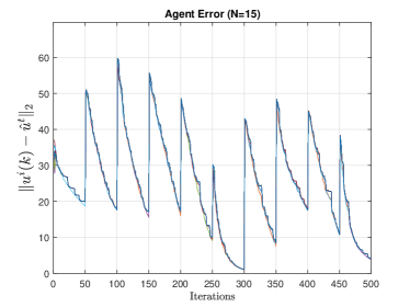
Figure 1: Plot of tracking error as a function of $k$ for $k$ from $0$ to $500$. The value of $\|u^{i}(k)-\hat{u}^{t}\|_{2}$ is shown for all $i\in[N]$.

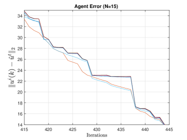
Figure 2: Zoomed-in plot of Figure 1 showing the tracking error as a function of $k$ for all $N=15$ agents. The periods of descent are when agents compute and communicate, leading to better tracking of their fixed point at that time. Flat areas are where agents either do not compute or communicate, thereby completing no cycles and making no progress in reducing tracking error.

VI-B Feedback Optimization with Measurement Noise

Secondly, we consider an example from the study of feedback optimization [34, 35, 36] in which the cost is on the deviation of the output of a dynamical system from a reference trajectory. Consider the objective function

$$f(u,t)=\frac{1}{2}u^{T}Q(t)u+\frac{1}{2}\left(y(u)-r(t)\right)^{2},$$ (55)

where $Q(t)\in\mathbb{R}^{n\times n}$, $y:\mathbb{R}^{n}\rightarrow\mathbb{R}$ is the input-output map of the system, and $r(t)\in\mathbb{R}$ is the time-varying reference signal that $y$ must track. In feedback optimization we only have knowledge of an output measurement affected by noise. Therefore, the objective function that we can compute is

$$f(u,t)=\frac{1}{2}u^{T}Q(t)u+\frac{1}{2}\left(\hat{y}(u)-r(t)\right)^{2},$$ (56)

where $\hat{y}(u)=y(u)+n(t)$ is the noisy measurement of the input-output map and $n(t)\sim\mathcal{N}(0,{1000^{2}})$ is i.i.d..

Figure 3 shows that, even with measurements corrupted by noise, Algorithm 1 can still track time-varying fixed points to within a ball centered on them. For example, just before the $8^{th}$ switch, agents’ average tracking error is 1.192, which indicates close tracking even under noise. Similar to the previous example, the switching of objective functions causes a noticeable error that is quickly mitigated by subsequent communication cycles. This example goes beyond the analytical tracking guarantees provided above, and further characterization of Algorithm 1 with measurement noise is a direction for future research.

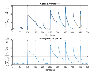
Figure 3: Plot of tracking error as a function of $k$ for all $N=15$ agents in the presence of noisy output measurements leading to a noisy gradient calculation. The sudden increases in error are due to the switching of objective functions similar to the previous example. Effects of asynchrony and noisy measurements can be observed; however, agents are still able to track their fixed point for all $t$ within a relatively small ball centered on them.

VII Conclusions

In this paper, we have proposed a totally asynchronous multi-agent algorithm for tracking time-varying fixed points that are solutions to time-varying optimization problems. We further optimized agents’ computations and communications to minimize dynamic regret when they are able to perform only a limited number of each type of operation. Next steps in this work include integrating the dynamics of agents into the update law for feedback optimization and analytically bounding tracking error when measurement noise is included in a feedback optimization setup.

-A Proof of Proposition 1

We prove that each of the four properties of Definition 2 is satisfied. First, consider the sets

$$U_{i}(s)\!=\!\left\{\!y_{i}\in\mathbb{R}^{n_{i}}\!:\!\left\|y_{i}-\hat{u}_{i}^{t}\right\|_{2}\leq q_{t}^{s}\max_{i\in[N]}\left\|u^{i}(\eta_{t-1})-\hat{u}^{t}\right\|_{2,\infty}\!\right\}.$$ (57)

Then, for $y=(y_{1},\ldots,y_{N})^{T}\in U_{1}(s)\times\cdots U_{N}(s)$, we have $N$ inequalities

$$\left\|y_{1}-\hat{u}_{1}^{t}\right\|_{2} \leq q_{t}^{s}\max_{i\in[N]}\left\|u^{i}(\eta_{t-1})-\hat{u}^{t}\right\|_{2,\infty}$$ (58)

$$\quad\quad\quad\quad\vdots$$ (59)

$$\left\|y_{N}-\hat{u}_{N}^{t}\right\|_{2} \leq q_{t}^{s}\max_{i\in[N]}\left\|u^{i}(\eta_{t-1})-\hat{u}^{t}\right\|_{2,\infty},$$ (60)

from which it follows that

$$\left\|y-\hat{u}^{t}\right\|_{2,\infty}\coloneqq\max_{i\in[N]}\left\|y_{i}-\hat{u}_{i}^{t}\right\|_{2}\leq q_{t}^{s}\max_{i\in[N]}\left\|u^{i}(\eta_{t-1})-\hat{u}^{t}\right\|_{2,\infty}.$$ (61)

Thus $y\in U_{1}(s)\times\cdots\times U_{N}(s)$ implies $y\in U(s)$ and

$$U_{1}(s)\times U_{2}(s)\times\cdots\times U_{N}(s)\subseteq U(s).$$ (62)

Now, consider $y\in U(s)$. Then,

$$\left\|y-\hat{u}^{t}\right\|_{2,\infty}\leq q_{t}^{s}\max_{i\in[N]}\left\|u^{i}(\eta_{t-1})-\hat{u}^{t}\right\|_{2,\infty}$$ (63)

and

$$\max_{i\in[N]}\left\|y_{i}-\hat{u}_{i}^{t}\right\|_{2}\leq q_{t}^{s}\max_{i\in[N]}\left\|u^{i}(\eta_{t-1})-\hat{u}^{t}\right\|_{2,\infty}.$$ (64)

This implies that, for all $i$, we have ${\left\|y_{i}-\hat{u}_{i}^{t}\right\|_{2}\leq q_{t}^{s}\max\limits_{i\in[N]}\left\|u^{i}(\eta_{t-1})-\hat{u}^{t}\right\|_{2,\infty}}$. Then $y\in U(s)$ implies that $y_{i}\in U_{i}(s)$ for all $i$, and thus $U(s)\subseteq U_{1}(s)\times U_{2}(s)\times\cdots\times U_{N}(s)$. This, combined with Equation (62), implies that Definition 2.1 holds.

For Definition 2.2, consider $y\in U(s+1)$. Then

$$\left\|y-\hat{u}^{t}\right\|_{2,\infty}\leq q_{t}^{s+1}\max_{i\in[N]}\left\|u^{i}(\eta_{t-1})-\hat{u}^{t}\right\|_{2,\infty}.$$ (65)

Since $q_{t}\in(0,1)$, we have

$$\left\|y-\hat{u}^{t}\right\|_{2,\infty}\leq q_{t}^{s+1}\max_{i\in[N]}\left\|u^{i}(\eta_{t-1})-\hat{u}^{t}\right\|_{2,\infty}\\ <q_{t}^{s}\max_{i\in[N]}\left\|u^{i}(\eta_{t-1})-\hat{u}^{t}\right\|_{2,\infty},$$ (66)

which implies $y\in U(s)$. Then $U(s+1)\subseteq U(s)$.

For Definition 2.3, we note that, because $q_{t}\in(0,1)$, we have $\lim\limits_{s\to\infty}q_{t}^{s}=0$. It immediately follows from the definition of $U(s)$ that $\lim_{s\to\infty}U(s)=\{\hat{u}^{t}\}$.

Towards satisfying Definition 2.4, we first observe that [21, Lemma 1] implies

$$\left\|I_{n}-\gamma_{t}H(u,t)\right\|_{2,\infty}\\ \leq\max_{i\in[N]}\left[\left\|I_{n_{i}}-\gamma_{t}H_{ii}(u,t)\right\|_{2}+\gamma_{t}\underset{j\neq i}{\sum_{j=1}^{n}}\left\|H_{ij}(u,t)\right\|_{2}\right].$$ (67)

Now consider the $i^{th}$ diagonal block of $I_{n}-\gamma_{t}H(u,t)$, which satisfies $\left[I_{n}-\gamma_{t}H(u,t)\right]_{ii}=I_{n_{i}}-\gamma_{t}H_{ii}(u,t)$. By Assumption 3, $H_{ii}(t)$ is symmetric. Then

$$\|I_{n_{i}}-\gamma_{t}H_{ii}(u,t)\|_{2}\\ =\max\Big{\{}\!\big{|}\lambda_{min}[I_{n_{i}}\!-\!\gamma_{t}H_{ii}(u,t)]\big{|},\big{|}\lambda_{max}[I_{n_{i}}\!-\!\gamma_{t}H_{ii}(u,t)]\big{|}\!\Big{\}}\\ =\max\Big{\{}\!\big{|}1-\gamma_{t}\lambda_{min}[H_{ii}(u,t)]\big{|},\big{|}1-\gamma_{t}\lambda_{max}[H_{ii}(u,t)]\big{|}\Big{\}}.$$ (68)

The upper bound on $\gamma_{t}$ gives ${1-\gamma_{t}\lambda_{min}\left[H_{ii}(u,t)\right]\geq 1-\gamma_{t}\lambda_{max}\left[H_{ii}(u,t)\right]}$. Then

$$\left\|I_{n_{i}}-\gamma_{t}H_{ii}(u,t)\right\|_{2}=1-\gamma_{t}\lambda_{min}[H_{ii}(u,t)].$$ (69)

Then we have

$$\underset{i\in\left[N\right]}{\max}\,\,\left\|I_{n_{i}}-\gamma_{t}H_{ii}(u,t)\right\|_{2}+\gamma_{t}\underset{j\neq i}{\sum_{j=1}^{n}}\left\|H_{ij}(u,t)\right\|_{2}$$ (70)

$$=\!\underset{i\in\left[N\right]}{\max}\,\,1\!-\!\gamma_{t}\Big{(}\lambda_{min}[H_{ii}(u,t)]\!-\!\underset{j\neq i}{\sum_{j=1}^{n}}\left\|H_{ij}(u,t)\right\|_{2}\!\Big{)}$$ (71)

$$\leq 1-\gamma_{t}\beta_{t}.$$ (72)

Using Equation (67), $\left\|I_{n}-\gamma_{t}H(u,t)\right\|_{2,\infty}\leq 1-\gamma_{t}\beta_{t}$.

For Definition 2.4, consider $\hat{u}^{t}=\Pi_{U}\left[\hat{u}^{t}-\gamma_{t}\nabla_{u}f\left(\hat{u}^{t},t\right)\right]$, i.e., $\hat{u}^{t}$ is a fixed point of the projected gradient descent mapping. Using the non-expansive property of the projection operator $\Pi_{U}\left[\cdot\right]$, we find

$$\left\|z_{i}-\hat{u}_{i}^{t}\right\|_{2}\\ =\left\|\Pi_{U_{i}}\left[y_{i}-\gamma_{t}\nabla_{u_{i}}f(y,t)\right]-\Pi_{U_{i}}\left[\hat{u}_{i}^{t}-\gamma_{t}\nabla_{u_{i}}f\left(\hat{u}^{t},t\right)\right]\right\|_{2}\\ \leq\left\|y_{i}-\gamma_{t}\nabla_{u_{i}}f(y,t)-\hat{u}_{i}^{t}+\gamma_{t}\nabla_{u_{i}}f\left(\hat{u}^{t},t\right)\right\|_{2}.$$ (73)

Using the Mean Value Theorem [37], we have

$$\nabla f(y,t)-\nabla f(\hat{u}^{t},t)=M(y,t)(y-\hat{u}^{t}),$$ (74)

where $M(y,t)\coloneqq\int_{0}^{1}H(\hat{u}^{t}+\tau(y-\hat{u}^{t}),t)d\tau$, which then gives

$$\left\|I_{n}-\gamma_{t}M(y,t)\right\|_{2,\infty}\leq 1-\gamma_{t}\beta_{t}.$$ (75)

Then we have

$$\left\|y_{i}-\gamma_{t}\nabla_{u_{i}}f(y,t)-\hat{u}_{i}^{t}+\gamma_{t}\nabla_{u_{i}}f\left(\hat{u}^{t},t\right)\right\|_{2}$$ (76)

$$\leq\underset{i\in\left[N\right]}{\max}\left\|y_{i}-\gamma_{t}\nabla_{u_{i}}f(y,t)-\hat{u}_{i}^{t}+\gamma_{t}\nabla_{u_{i}}f\left(\hat{u}^{t},t\right)\right\|_{2}$$ (77)

$$=\left\|y-\gamma_{t}\nabla_{u}f(y,t)-\hat{u}^{t}+\gamma_{t}\nabla_{u}f\left(\hat{u}^{t},t\right)\right\|_{2,\infty}$$ (78)

$$=\left\|y-\hat{u}^{t}-\gamma_{t}\left(\nabla_{u}f(y,t)-\nabla_{u}f\left(\hat{u}^{t},t\right)\right)\right\|_{2,\infty}$$ (79)

$$=\left\|y-\hat{u}^{t}-\gamma_{t}M(y,t)\left(y-\hat{u}^{t}\right)\right\|_{2,\infty}$$ (80)

$$\leq\left\|I_{n}-\gamma_{t}M(y,t)\right\|_{2,\infty}\left\|y-\hat{u}^{t}\right\|_{2,\infty}$$ (81)

$$\leq\left(1-\gamma_{t}\beta_{t}\right)\left\|y-\hat{u}^{t}\right\|_{2,\infty}.$$ (82)

Therefore, because the bounds on $\gamma_{t}$ imply $1-\gamma_{t}\beta_{t}\in(0,1)$, $y\in U(s)$ implies that ${z_{i}\in U_{i}(s+1)}$.

References

- [1] S. M. Fosson, “Online optimization in dynamic environments: a regret analysis for sparse problems,” in 2018 IEEE Conference on Decision and Control (CDC). IEEE, 2018, pp. 7225–7230.
- [2] F. Y. Jakubiec and A. Ribeiro, “D-map: Distributed maximum a posteriori probability estimation of dynamic systems,” IEEE Transactions on Signal Processing, vol. 61, no. 2, pp. 450–466, 2013.
- [3] S. M. Fosson, “Centralized and distributed online learning for sparse time-varying optimization,” IEEE Transactions on Automatic Control, vol. 66, no. 6, pp. 2542–2557, 2021.
- [4] O. Arslan and D. E. Koditschek, “Exact robot navigation using power diagrams,” in 2016 IEEE International Conference on Robotics and Automation (ICRA), 2016, pp. 1–8.
- [5] A. Hauswirth, I. Subotić, S. Bolognani, G. Hug, and F. Dörfler, “Time-varying projected dynamical systems with applications to feedback optimization of power systems,” in 2018 IEEE Conference on Decision and Control (CDC), 2018, pp. 3258–3263.
- [6] Y. Tang, K. Dvijotham, and S. Low, “Real-time optimal power flow,” IEEE Transactions on Smart Grid, vol. 8, no. 6, pp. 2963–2973, 2017.
- [7] T. Zheng, J. Simpson-Porco, and E. Mallada, “Implicit trajectory planning for feedback linearizable systems: A time-varying optimization approach,” 2020.
- [8] Y. Tian, Y. Sun, and G. Scutari, “Asy-sonata: Achieving linear convergence in distributed asynchronous multiagent optimization,” in 2018 56th Annual Allerton Conference on Communication, Control, and Computing (Allerton), 2018, pp. 543–551.
- [9] A. Nedic, “Asynchronous broadcast-based convex optimization over a network,” IEEE Transactions on Automatic Control, vol. 56, no. 6, pp. 1337–1351, 2011.
- [10] F. Iutzeler, P. Bianchi, P. Ciblat, and W. Hachem, “Asynchronous distributed optimization using a randomized alternating direction method of multipliers,” in 52nd IEEE Conference on Decision and Control, 2013, pp. 3671–3676.
- [11] J. C. Duchi, A. Agarwal, and M. J. Wainwright, “Dual averaging for distributed optimization: Convergence analysis and network scaling,” IEEE Transactions on Automatic control, vol. 57, no. 3, pp. 592–606, 2011.
- [12] K. I. Tsianos and M. G. Rabbat, “Distributed dual averaging for convex optimization under communication delays,” in 2012 American Control Conference (ACC), 2012, pp. 1067–1072.
- [13] D. P. Bertsekas and J. N. Tsitsiklis, Parallel and Distributed Computation: Numerical Methods. USA: Prentice-Hall, Inc., 1989.
- [14] T.-H. Chang, M. Hong, W.-C. Liao, and X. Wang, “Asynchronous distributed admm for large-scale optimization—part i: Algorithm and convergence analysis,” IEEE Transactions on Signal Processing, vol. 64, no. 12, pp. 3118–3130, 2016.
- [15] F. Mansoori and E. Wei, “Superlinearly convergent asynchronous distributed network newton method,” in 2017 IEEE 56th Annual Conference on Decision and Control (CDC), 2017, pp. 2874–2879.
- [16] P. Tseng, D. P. Bertsekas, and J. N. Tsitsiklis, “Partially asynchronous, parallel algorithms for network flow and other problems,” SIAM Journal on Control and Optimization, vol. 28, no. 3, pp. 678–710, 1990.
- [17] J. N. Tsitsiklis, “On the stability of asynchronous iterative processes,” in 1986 25th IEEE Conference on Decision and Control, 1986, pp. 1617–1621.
- [18] J. Tsitsiklis, D. Bertsekas, and M. Athans, “Distributed asynchronous deterministic and stochastic gradient optimization algorithms,” IEEE Transactions on Automatic Control, vol. 31, no. 9, pp. 803–812, 1986.
- [19] D. P. Bertsekas, “Distributed asynchronous computation of fixed points,” Mathematical Programming, vol. 27, no. 1, pp. 107–120, 1983.
- [20] K. R. Hendrickson and M. T. Hale, “Towards totally asynchronous primal-dual convex optimization in blocks,” in 2020 59th IEEE Conference on Decision and Control (CDC), 2020, pp. 3663–3668.
- [21] M. Ubl and M. T. Hale, “Totally asynchronous large-scale quadratic programming: Regularization, convergence rates, and parameter selection,” 2020.
- [22] K. Yazdani and M. Hale, “Asynchronous parallel nonconvex optimization under the polyak-Łojasiewicz condition,” IEEE Control Systems Letters, vol. 6, pp. 524–529, 2022.
- [23] B. M. Assran, A. Aytekin, H. R. Feyzmahdavian, M. Johansson, and M. G. Rabbat, “Advances in asynchronous parallel and distributed optimization,” Proceedings of the IEEE, vol. 108, no. 11, pp. 2013–2031, 2020.
- [24] H. R. Feyzmahdavian and M. Johansson, “Asynchronous iterations in optimization: New sequence results and sharper algorithmic guarantees,” arXiv preprint arXiv:2109.04522, 2021.
- [25] A. Simonetto, A. Mokhtari, A. Koppel, G. Leus, and A. Ribeiro, “A class of prediction-correction methods for time-varying convex optimization,” IEEE Transactions on Signal Processing, vol. 64, no. 17, pp. 4576–4591, 2016.
- [26] A. Simonetto and E. Dall’Anese, “Prediction-correction algorithms for time-varying constrained optimization,” IEEE Transactions on Signal Processing, vol. 65, no. 20, pp. 5481–5494, 2017.
- [27] A. Simonetto, A. Mokhtari, A. Koppel, G. Leus, and A. Ribeiro, “A decentralized prediction-correction method for networked time-varying convex optimization,” in 2015 IEEE 6th International Workshop on Computational Advances in Multi-Sensor Adaptive Processing (CAMSAP), 2015, pp. 509–512.
- [28] A. Bernstein and E. Dall’Anese, “Asynchronous and distributed tracking of time-varying fixed points,” in 2018 IEEE Conference on Decision and Control (CDC). IEEE, 2018, pp. 3236–3243.
- [29] S. Boyd, S. P. Boyd, and L. Vandenberghe, Convex optimization. Cambridge university press, 2004.
- [30] C. K. Tan, M. J. Tippett, and J. Bao, “Model predictive control with non-uniformly spaced optimization horizon for multi-timescale processes,” Computers and Chemical Engineering, vol. 84, pp. 162–170, 2016. [Online]. Available: https://www.sciencedirect.com/science/article/pii/S0098135415002719
- [31] W. K. Weiss, D. Burns, and M. Guay, “Realtime optimization of mpc setpoints using time-varying extremum seeking control for vapor compression machines,” 2014.
- [32] A. Hauswirth, S. Bolognani, G. Hug, and F. Dörfler, “Timescale separation in autonomous optimization,” IEEE Transactions on Automatic Control, vol. 66, no. 2, pp. 611–624, 2021.
- [33] M. T. Hale, A. Nedić, and M. Egerstedt, “Asynchronous multiagent primal-dual optimization,” IEEE Transactions on Automatic Control, vol. 62, no. 9, pp. 4421–4435, 2017.
- [34] M. Colombino, E. Dall’Anese, and A. Bernstein, “Online optimization as a feedback controller: Stability and tracking,” IEEE Transactions on Control of Network Systems, vol. 7, no. 1, pp. 422–432, 2019.
- [35] A. Bernstein, E. Dall’Anese, and A. Simonetto, “Online primal-dual methods with measurement feedback for time-varying convex optimization,” IEEE Transactions on Signal Processing, vol. 67, no. 8, pp. 1978–1991, 2019.
- [36] S. Menta, A. Hauswirth, S. Bolognani, G. Hug, and F. Dörfler, “Stability of dynamic feedback optimization with applications to power systems,” in 2018 56th Annual Allerton Conference on Communication, Control, and Computing (Allerton). IEEE, 2018, pp. 136–143.
- [37] T. M. Flett, “2742. a mean value theorem,” The Mathematical Gazette, vol. 42, no. 339, pp. 38–39, 1958.