AGN orientation through the spectroscopic correlations and model of dusty cone shell

Abstract

The differences between Narrow Line Seyfert 1 galaxies (NLS1s) and Broad Line AGNs (BLAGNs) are not completely understood; it is thought that they may have different inclinations and/or physical characteristics. The FWHM(H$\beta$)–luminosities correlations are found for NLS1s and their origin is the matter of debate. Here we investigated the spectroscopic parameters and their correlations considering a dusty, cone model of AGN. We apply a simple conical dust distribution (spreading out of broad line region, BLR), assuming that the observed surface of the model is in a good correlation with MIR emission. The dusty cone model in combination with a BLR provides the possibility to estimate luminosity dependence on the cone inclination. The FWHM(H$\beta$)–luminosities correlations obtained from model in comparison with observational data show similarities which may indicate the influence of AGN inclination and structure to this correlation. An alternative explanation for FWHM(H$\beta$)–luminosities correlations is the selection effect by the black hole mass. These FWHM(H$\beta$)–luminosities correlations may be related to the starburst in AGNs, as well. The distinction between spectral properties of the NLS1s and BLAGNs could be caused by multiple effects: beside physical differencies between NLS1s and BLAGNs (NLS1s have lighter black hole mass than BLAGNs), inclination of the conical AGN geometry may have important role as well, where NLS1s may be seen in lower inclination angles.

1 Introduction

A broad line region (BLR) in active galactic nuclei (AGNs) is believed to be formed close to the black hole (several hundreds of light days in radius; GRAVITY Collaboration et al., 2018) where the gas velocity is up to several thousands km s^-1. The BLR emits broad lines which are mainly broadened due to the violent emitting gas motion around a supermassive black hole. The AGN unification model (Antonucci, 1993; Urru & Padovani, 1995) relies to the existance of the dusty torus of the size of $\sim$10 pc (Tristram & Schartmann, 2011) around the accretion disc. Out of the dusty torus, there is the narrow line region, where the narrow emission lines arise. According to the unification model, the AGNs Type 1 are seen nearly face on (small inclination angles of BLR, $i$) and these objects have broad and narrow lines in their spectra. Unlike them, the AGNs Type 2 are seen under larger inclination ($i\approx$ 90$\degree$), their BLR is observed through the torus, therefore their BLR is not seen, only narrow emission lines can be observed in their spectra and they are known as obscured AGNs. Some recent mid-infrared (MIR) studies require the polar cones of dust, stretching out from the central source (Hönig, 2019) instead (or together with) preveously presumed dusty torus. Recently, MIR observations resolved dusty and molecular structures in polar directions, on scales from 10 to 100 pc (García-Burrilo et al., 2014; Gallimore et al., 2016; Alonso-Herrero et al., 2018; Asmus, 2019; Alonso-Herrero et al., 2021; Buat et al., 2021; Toba et al., 2021), while the theoretical works confirmed that these structures may be from dusty wind driven by the radiation pressure (see Stalevski et al., 2019, and references therein, hereafter S19). The observed AGN outer half-opening cone angles, $\theta\texttt{=}$30-60$\degree$ (Bae & Woo, 2016) are similar to torus presumed half-opening angles of 30-60$\degree$ (Marin et al., 2015). Finding that the MIR emission in AGNs is probably from dust embedded in polar outflows in the narrow line region instead of in the torus (Zhang et al., 2013) may change much in the AGN understanding, as well as in the comprehension of the differences between Narrow line Seyfert 1 (NLS1) galaxies and Broad Line AGNs (BLAGNs).

Osterbrock & Pogge (1985) and Goodrich (1989) defined a new class of AGN, NLS1, that have full width at half maximum of broad permitted line H$\beta$, FWHM(H$\beta$) $<$2000 km s^-1 and flux ratio of total [O III]$\lambda$5007 to total H$\beta<$ 3. These AGNs have notable distinctions from BLAGNs, such as narrower broad emission lines, lighter black hole mass (M_BH) and lower luminosities (Sani et al., 2010; Schmidt et al., 2016), higher polycyclic aromatic hydrocarbon (PAH) presence, denser BLR clouds, possibly lower inclination, more star formation, have more bars and dust spirals, higher accretion rate, strong optical and UV Fe II emission, weak [O III], lower optical variability and more rapid X-ray variability (Boroson & Green, 1992; Grupe et al., 1999; Rakshit & Stalin, 2017; Lakićević et al., 2018). Some studies suggest that NLS1s and BLAGNs have different geometry (Baldi et al., 2016; Liu et al., 2016). On the other hand, there are indications that NLS1s are regular Seyfert galaxies at an early stage of evolution where black hole is still growing (Mathur, 2000, 2001; Jin et al., 2012a), and that NLS1s possibly have the same characteristic as BLAGNs, but they are only seen under the different inclination angles (Nagao et al., 2000; Zhang & Wu, 2002; Decarli et al., 2008; Rakshit et al., 2017). Recently there are various proofs that some NLS1s show blazar characteristics (Järvelä et al., 2015; Yang, 2018). Nevertheless, Järvelä et al. (2017) suggested that NLS1s and BLAGNs have a different enviromental density and distribution, therefore they should not be unified by orientation. Some of foregoing characteristics can indeed be explained by lower inclination and lower M_BH of NLS1s, as we discuss in this paper.

NLS1s show the correlation between FWHM(H$\beta$) and several optical and MIR line and continuum luminosities, while BLAGNs do not have that characteristic (Lakićević et al., 2018, hereafter La18) and the cause of that is not certain. Järvelä et al. (2015) also found somewhat weaker (with a correlation coefficient of $\sim$0.3) trends FWHM(H$\beta$)-luminosities (optical, MIR and radio) for NLS1s. Popović & Kovačević (2011) found that the AGNs with stronger starburst contribution have the correlation between FWHM(H$\beta$) and optical luminosity, while the other AGNs do not have this trend. This finding is similar to the one for NLS1 correlations (see above), as starburst objects are often connected with NLS1s. Boller et al. (2001) noticed anticorrelation between soft X-ray excess strength (0.1–2.4 keV) and FWHM(H$\beta$) and between hard continuum slope (2–10 keV) with FWHM(H$\beta$), for NLS1s. Jarvis & McLure (2006) noted strong correlation between radio spectral index (known to be connected with the source orientation) and FWHM of broad lines H$\beta$ and Mg II. AGNs with FWHM(H$\beta$)$>$4000 km s^-1 have a larger redshifted very broad line region component of H$\beta$ (velocities$\sim$5000 km ^-1) (see Sulentic et al., 2002; Kovačević et al., 2010).

If there is not any dust extinction (absorption and/or scaterring) within an AGN, then the angle of view of AGN would not be important since all photons would arrive to the observer. The angle-dependent obscuration is needed for AGN unification understanding (Hönig, 2019). In estimation of the luminosity received from the certain object under different $i$, we are interested in its geometry, size of the observed surface and optical depth. Here we tested if the inclination, observed surface and the optical depth could determine the luminosity of AGNs.

Inclination of AGNs may not only influence the type of AGNs we detect, but also significantly affects the estimation of M_BH when FWHM of broad emission lines is used, as well as it affects some reverberation-based M_BH calculations, especially for the objects with the narrowest emission lines (Collin et al., 2006). Even $M-\sigma$* relation (between M_BH and stellar velocity dispersion) is contaminated by the inclination influence, as inclination may affect measured velocity dispersions by 30$\%$, and consequently M_BH may be affected up to 1 dex, where face-on objects have lower, and edge-on sistematicaly higher $\sigma$*, due to contamination by disc stars (Bellovary et al., 2014).

The aim of this paper is to explain spectral characteristics and correlations between spectral parameters of the AGNs by the inclination calculated from spectroscopic parameters in combination with the specific conical distribution of dust which is observed in some AGNs. For that purpose, we involve dusty cone models and we test the changes in spectral properties for different angles of view.

In Section 2 we explain the dataset and the used procedure. In Section 3, the major plots and results are shown. In Section 4 the implications of obtained relations are discussed. In Section 5, the concluding remarks are listed. Cosmological parameters used in this work are $\Omega_{m}\texttt{=}$0.3, $\Lambda\texttt{=}$ 0.7 and H${}_{0}\texttt{=}$ 70 km s^-1 Mpc^-1.

2 Data and Methods

For this research we needed the sample of the AGN Type 1 spectra for which: a) M_BH is calculated with some method independent of FWHM(H$\beta$) (in order to calculate inclination $i$, see Eq. 1), b) for which the MIR spectra are available in order to investigate the correlations of the MIR spectral properties with $i$. Therefore, the data used in this investigation is composed from the two datasets of Type 1 AGNs, Zhang & Wu (2002) and Afanasiev et al. (2019) for which there are available certain spectroscopic parameters needed to calculate the inclination. Data from Zhang & Wu (2002) are chosen with the same purpose, while here that sample is enriched with the data from Afanasiev et al. (2019) and one object from Shapovalova et al. (2012). Data from Afanasiev et al. (2019) indicated equatorial scattering. M_BHs are calculated using stellar velocity dispersions or using polarization in broad lines. Additionally, these objects also have available Spitzer spectra. Reduced Spitzer Space Telescope spectra from Infrared Spectrograph (IRS) instrument, in low-resolution ($\sim$60-127) and/or high-resolution ($\sim$600) are downloaded from the Combined Atlas of Sources with Spitzer IRS Spectra, CASSIS (Lebouteiller et al., 2011, 2015) for whole dataset. The dataset used in this paper consists of 56 (28 NLS1s and 28 BLAGNs) low redshift AGNs for which some spectral characteristics are shown in Fig. 1.

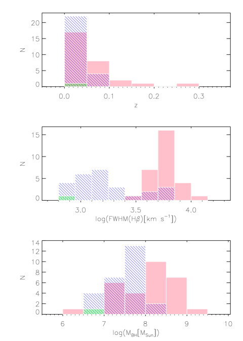
Figure 1: The histograms of major spectral parameters for the AGN dataset used in this paper. The histograms for objects from Afanasiev et al. (2019) are coloured with pink, the histograms for objects from Zhang & Wu (2002) are filled with blue lines, while the object from Shapovalova et al. (2012) is filled with green.

Optical parameters such as orbital velocities ($\sigma_{V}$, estimated from broad lines), FWHM(H$\beta$), and BLR radius (R_BLR), are taken from aforementioned three papers. There, R_BLR is calculated by reverberation mapping, while $\sigma_{V}$ was calculated from FWHM(H$\beta$), such that FWHM(H$\beta$)$\approx$2.355$\sigma_{V}$.

The M_BHs of objects from the sample are taken from the aforementioned three papers as well. For the objects from Afanasiev et al. (2019) and from Shapovalova et al. (2012), M_BHs are derived using polarization in broad lines, while for the objects from Zhang & Wu (2002), M_BHs are obtained using stellar velocity dispersion.

For the objects from Zhang & Wu (2002) and Shapovalova et al. (2012) inclination is calculated in the same way as in Afanasiev et al. (2019), according to the equation:

$$\sin\left(i\right)\texttt{=}\sigma_{V}\sqrt{\frac{R_{\rm BLR}}{M_{\rm BH}G}},$$ (1)

where $G$ is gravitational constant. The spectroscopic data used in this paper are given in the Tables 1, 2 and 3. For the data from Afanasiev et al. (2019) $\Delta\sigma_{V}$ is taken from that paper, while for the rest of the data it is estimated as 4%, as that is the most common value in the histogram of the data from Afanasiev et al. (2019). $\Delta$FWHM(H$\beta$) and $\Delta$R_BLR are taken from Afanasiev et al. (2019), Zhang & Wu (2002), or estimated as 4% and 20%, respectively (similarly as for $\Delta\sigma_{V}$). $\Delta$log(M_BH) is from Afanasiev et al. (2019) or estimated as 3.5%, similarly as for $\Delta\sigma_{V}$. For the equability of two datasets, the errors of inclination were found as

$$\Delta i\texttt{=}\frac{1}{2}tg\left(i\right)\times\left(\frac{\Delta R}{R}\texttt{+}\frac{2\Delta\sigma_{V}}{\sigma_{V}}\texttt{+}\frac{\Delta M_{\rm BH}}{M_{\rm BH}}\right),$$ (2)

for the whole sample.

Table 1: The name of object, coordinates and redshifts are given in columns 1, 2, 3 and 4; FWHM(H$\beta$), its reference, $\Delta$FWHM(H$\beta$) and its reference in columns 5, 6, 7 and 8, while equivalent width (EW) of PAH at 7.7 $\mu$m and its uncertainty is given in columns 9 and 10. The data are compiled from the datasets from Afanasiev et al. (2019) (A19), Zhang & Wu (2002) (Z02) and Shapovalova et al. (2012) (S12). Only a portion of this table is shown here to demonstrate its form and content.

NAME	RA[$\degree$]	Dec[$\degree$]	z	FWHM(H$\beta$)[km s-1]	ref	$\Delta$FWHM(H$\beta$)[km s-1]	ref	EW7.7[nm]	$\Delta$EW7.7[nm]
(1)	(2)	(3)	(4)	(5)	(6)	(7)	(8)	(9)	(10)
Mrk 335	1.581339	20.202914	0.026	5306	A19	200.2	A19	1.0	0.2213
Mrk 1501	2.629191	10.974862	0.089	5617	A19	195.5	A19	12.0	3.791028
Mkn 1148	12.978167	17.432917	0.064	4724	A19	353.2	A19	6.3	1.0538955
I Zw1	13.395585	12.69339	0.059	5011	A19	280.3	A19	14.0	2.32988

Table 2: The name of object, PAH fraction – RPAH (see the text), its uncertainty, L6, its error, L12, its error, log(M_BH[M_⊙]) and its uncertainty and the reference for the mass. Only a portion of this table is shown here to demonstrate its form and content.

NAME	RPAH	$\Delta$RPAH	L6[erg s-1]	$\Delta$L6[erg s-1]	L12[erg s-1]	$\Delta$L12[erg s-1]	log(MBH[M⊙])	$\Delta$log(MBH[M⊙])	ref
(1)	(2)	(3)	(4)	(5)	(6)	(7)	(8)	(9)	(10)
Mrk 335	0.002	0.071	8.117$\times$1043	2.831$\times$1042	7.197$\times$1043	2.516$\times$1042	7.49	0.25	A19
Mrk 1501	0.002	0.138	3.783$\times$1044	2.641$\times$1043	3.502$\times$1044	2.439$\times$1043	8.57	0.26	A19
Mkn 1148	6.83$\times$10-4	0.142	4.236$\times$1043	2.030$\times$1042	3.396$\times$1043	1.639$\times$1042	8.69	0.18	A19
I Zw1	0.0	0.043	7.214$\times$1044	1.727$\times$1043	9.264$\times$1044	2.226$\times$1043	7.46	0.3	A19

Table 3: The name of object, R_BLR, its reference, $\Delta$R_BLR, its reference, calculated inclination $i$, $\Delta i$, AGN type, reference, luminosity at the peak of the 7.7 $\mu$m feature and its uncertainties are in columns 1-11. The AGN classification is taken from various literature: Marziani et al. (1993) (M93), Gonçalves et al. (1999) (G99), Klimek et al. (2004) (K04), Nikołajuk et al. (2009) (N09), Bian et al. (2010) (B10), Sani et al. (2010) (S10), Véron-Cetty et al. (2010) (VC10), Berton et al. (2015) (B15), Markowitz et al. (2014) (Mar14), Marinello et al. (2016) (M16). Only a portion of this table is shown here to demonstrate its form and content.

NAME	RBLR[l.d.]	ref	$\Delta$RBLR [l.d.]	ref	$i$	$\Delta i$	Type	ref	log($\nu$L7.7)[erg s-1]	$\Delta$log($\nu$L7.7)[erg s-1]
(1)	(2)	(3)	(4)	(5)	(6)	(7)	(8)	(9)	(10)	(11)
Mrk 335	15.7	A19	3.0	A19	44.5	0.147	NLS1	S10	41.661	39.045
Mrk 1501	72.3	A19	5.4	A19	28.8	0.048	NLS1	B15	41.895	41.173
Mkn 1148	34.3	A19	0.1	A19	13.7	0.021	BLAGN	VC10	40.669	39.071
I Zw1	18.7	A19	2.5	A19	45.4	0.145	NLS1	S10	–	–

The deblendIRS (see Hernán-Caballero et al, 2015) script was used for the decomposition of Spitzer spectra to the AGN, PAH and stellar components (for example see Fig. 8 in Lakićević et al., 2017). The MIR spectral parameters, monochromatic luminosities at 6 and 12 $\mu$m, L6 and L12, respectively and RPAH (fractional contribution of PAH component to the integrated 5-15 $\mu$m luminosity) are obtained using deblendIRS. The equivalent width (EW) of PAH at 7.7 $\mu$m are measured using Starlink Dipso package. The PAHs at 7.7 $\mu$m are chosen among other PAHs from the available spectra because of high intensity and because they do not coincide with significant MIR spectral lines.

2.1 The hyperboloid and disc projection surfaces

In order to estimate the luminosity received from an AGN observed from the different inclinations ($i$), we are interested in its observed surface size, its density, opacity and optical depth. The optical depth ($\tau_{\lambda}$) depends on the path through the object ($s$), density ($\rho$) and the absorption coefficient $\kappa_{\lambda}$ (opacity), such that:

$$\alpha_{\lambda}\texttt{=}\rho\kappa_{\lambda}$$ (3)

and

$$\tau_{\lambda}\texttt{=}\int\alpha_{\lambda}\mathop{}\!\mathrm{d}s\texttt{=}\alpha_{\lambda}s,$$ (4)

assuming that the extinction coefficient $\alpha_{\lambda}$ is constant through the path, while $s$ depends on the viewing angle (see below). The observed intensity from the object, $I$, depends on the $\tau_{\lambda}$ as

$$I\texttt{=}I_{0}e^{-\tau},$$ (5)

where $I_{0}$ is the initial intensity from that object.

In the case of classical torus model of the AGNs (found based on optical observations) the observed surface of an AGN would decrease with the inclination angle, as the circle of view is becoming the ellipse and luminosities would drop with $i$. Therefore, we used dusty cone models of active galaxies, such as a model made for Circinus galaxy (see S19), as the luminosities have considerable increase with $i$ (for lower inclinations), which may cause FWHM(H$\beta$)–luminosities relations. We check if dusty cone models are related to the correlations between FWHM(H$\beta$) and spectral characteristics. In the model for Circinus galaxy presented in S19 (Section 3.1.1), MIR observations of this AGN are explained as one sheet dusty hyperboloid shell with a thin dusty disc, on parsec scales. This model does not consider dusty torus that is modeled by SKIRTOR in S19 (Section 3.1.2), which is one of the most used models in the literature. The conical body is limited with two hyperboloids which have the equations:

$$\frac{x^{2}}{a^{2}}\texttt{+}\frac{y^{2}}{b^{2}}-\frac{z^{2}}{c^{2}}\texttt{=}1,$$ (6)

where $a\texttt{=}b$ (radial symmetry), therefore

$$\frac{(x^{2}\texttt{+}y^{2})}{a^{2}_{1}}-\frac{z^{2}}{c_{1}^{2}}\texttt{=}1,$$ (7)

and

$$\frac{(x^{2}\texttt{+}y^{2})}{a^{2}_{2}}-\frac{z^{2}}{c_{2}^{2}}\texttt{=}1,$$ (8)

where $a_{1}\texttt{=}0.2$ pc for the inner and $a_{2}\texttt{=}0.6$ pc for the outer hyperboloid (from S19 model), while parameters $c_{1}$ and $c_{2}$ are 0.35 and 1.04, respectively ($c_{1,2}\texttt{=}a_{1,2}\times$ tan(90$\degree-\theta)$), for the cone angle $\theta\texttt{=}$30$\degree$). The hyperboloid height is taken to be $h\texttt{=}$6.23 pc, dusty disc radius is $D\texttt{=}$3 pc, while angle of dusty disc is $\Delta_{{\rm disc}}\texttt{=}$5$\degree$ (see Fig. 1 in S19). The model is rotated around the y-axis and in the Figs. 2 and 3 are presented the projected surfaces to the plane of observer of a given model seen under the different inclination angles (2–90$\degree$).

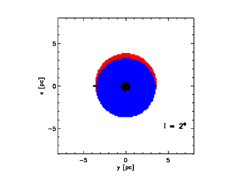
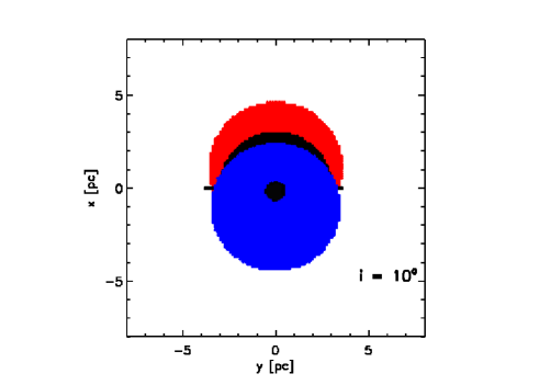
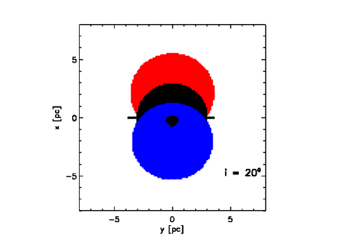
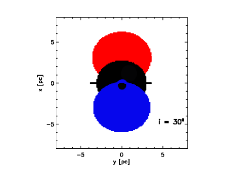
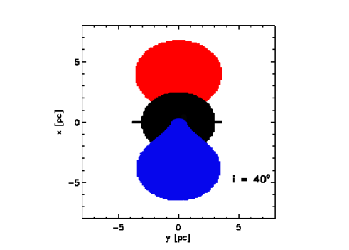
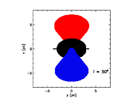
Figure 2: The projections of the polar dusty wind in a form of a hyperboloid shell with thin dusty disc to the plane of observer, for the various inclination angles (written in each panel). The two cones are coloured blue and red, while the dusty disc is black.

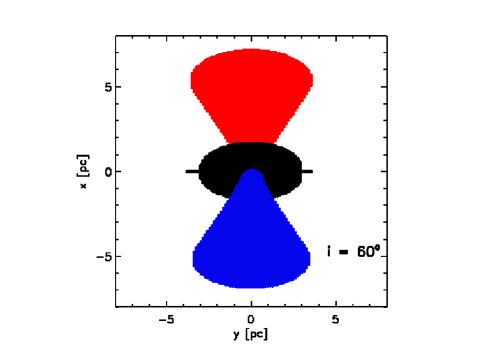
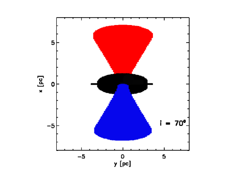
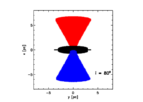
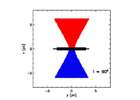
Figure 3: The same as in Fig. 2, but on the higher inclinations.

In this analysis we assume that the BLR is flattened and coplanar with the dusty disc, or in other words that the axis of symmetry of a dusty cone is perpendicular to the flattened BLR.

A Monte Carlo simulation with 10000 points in 2D space is performed in order to calculate the surfaces of the projections (in pc²) of the model to the plane of observer, for the various angles of inclination (as seen in the Figs. 2 and 3). The resulting surfaces of the hyperboloid and the dusty disc components are given in the Table 4, in the second and the third column, respectively. In the fourth column, these two surfaces are added. Errors of Monte Carlo surface estimation were estimated to be 0.1729%.

Table 4: Modeled surfaces for different inclinations: Inclinations (column 1); the surfaces of the projections of the hyperboloid and dusty disc to the plane of observer under the different inclination angles are in columns 2 and 3 ($S_{{\rm hyp}}$ and $S_{{\rm ddisc}}$); while in column 4 there is $S_{{\rm hyp\texttt{+}ddisc}}$ (added surfaces of hyperboloid and dusty disc).

i [$\degree$]	$S_{{\rm hyp}}$[pc2]	$S_{{\rm ddisc}}$[pc2]	$S_{{\rm hyp\texttt{+}ddisc}}$[pc2]
(1)	(2)	(3)	(4)
2	41.73$\pm$0.07	28.14$\pm$0.05	69.87$\pm$0.09
10	52.74$\pm$0.09	27.91$\pm$0.05	80.65$\pm$0.10
20	64.00$\pm$0.11	26.98$\pm$0.05	90.98$\pm$0.12
30	68.61$\pm$0.12	25.36$\pm$0.04	93.97$\pm$0.13
40	68.10$\pm$0.12	23.27$\pm$0.04	91.37$\pm$0.13
50	66.05$\pm$0.11	20.74$\pm$0.04	86.79$\pm$0.12
60	63.23$\pm$0.11	16.64$\pm$0.03	79.87$\pm$0.11
70	60.16$\pm$0.10	12.29$\pm$0.02	72.45$\pm$0.10
80	55.81$\pm$0.10	8.19$\pm$0.01	64.00$\pm$0.10
90	52.33$\pm$0.09	3.78$\pm$0.006	56.11$\pm$0.09

Afterwards, we applied some different possible cone models without a disc (since the disc would not change the observed surfaces much for large heights). The expected cone angles for AGNs are $\theta\texttt{=}$30-60$\degree$. Here, adopted cone height is 40 pc (although some observed cone heights are order of magnitude higher). We will show that the shape of the dependence of the projection surface (to the plane of the observer) from $i$ does not depend on the cone hight (while the projection surfaces depend on cone height).

3 Results

In Section 3.1 we find the correlations among spectral parameters and $i$ (for the dataset in Tables 1, 2 and 3). In Sections 3.2 and 3.3 we tried to estimate the luminosities calculated using the dusty cone models seen under different $i$, and compare their dependence on $i$ with the dependence of the real luminosities from FWHM(H$\beta$).

3.1 The correlations of spectroscopic parameters with $i$

The dependence FWHM(H$\beta$)-$i$ is expected to exist, as the projection of the rotational velocity of the matter from accretion disc to the direction to the observer grows with $i$. Therefore, the other implications of this relation are considered. The relation between inclination, $i$ and FWHM(H$\beta$) of Type 1 AGNs dataset (similarly as in Zhang & Wu, 2002) is also present here for somewhat different sample (see Fig. 4). Note that in our previous works we did not consider the errors of parameters (as they were not always available and homogeneous). In order to see how the strength of correlation would be changed, we represent results from correlation analysis both with and without taking into account errors. In Fig. 4 are given linear fitting without errors included (linfit in IDL for all objects and for NLS1s and BLAGNs separately), together with the fitting using a Bayesian method of linear regression (linmix_err in IDL, for all objects and for NLS1s and BLAGNs separately) that accounts for the errors of each parameter (method is described in Kelly, 2007). All correlations are shown in the Table 5. One can notice that for BLAGNs there are no trends. In the Bayesian fittings Markov chains were created using the Metropolis-Hastings algorithm. The fitting parameters are similar for these three kinds of fitting (the three pair of lines overlap).

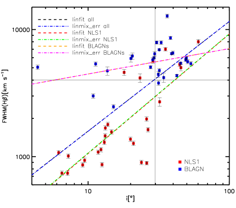
Figure 4: The relations between $i$ and FWHM(H$\beta$) for dataset of Type 1 AGN, for all objects and for NLS1s and BLAGNs separately, including and without errors included (see the legend). The correlations are given in the Table 5. Horizontal line denotes FWHM(H$\beta$) =4000 km s^-1, and vertical line denotes $i\texttt{=}$29.72$\degree$. Red colour marks NLS1s, while blue colour presents BLAGNs.

Table 5: Fitting results for Fig. 4: A – constant, B – slope, R – Pearson correlaton coefficient and P value (without errors included) and: A_e, B_e and R_e correlaton coefficient (with errors included), for all objects and for NLS1s and BLAGNs separatelly. As it is shown in the last column, for BLAGNs there are no trends.

	A	B	R	P	Ae	Be	Re	Related?
All	0.86$\pm$0.13	2.34$\pm$0.17	0.68	$<$10-5	0.86$\pm$0.13	2.33$\pm$0.18	0.68$\pm$0.07	yes
NLS1s	0.94$\pm$0.15	2.08$\pm$0.18	0.78	$<$10-5	0.94$\pm$0.16	2.08$\pm$0.20	0.81$\pm$0.08	yes
BLAGNs	3.45$\pm$0.15	0.20$\pm$0.10	0.36	0.062	3.45$\pm$0.16	0.20$\pm$0.11	0.36$\pm$0.18	no

The known relation of FWHM(H$\beta$) vs. fractional PAH contribution to Spitzer spectra, RPAH (Lakićević et al., 2017), is shown in Fig. 5. The correlation parameters without errors included (full line) and with errors accounted (dotted line) are given on the plot and shown in the Table 6. One can notice that without including uncertainties, the slope is steeper. La18 found this trend for NLS1 objects, while for BLAGNs it did not exist.

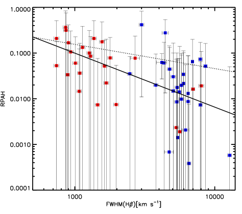
Figure 5: A relation between FWHM(H$\beta$) and RPAH for Type 1 AGNs dataset from this paper. Full line is fit without uncertainties accounted (y=(-1.18$\pm$0.24)x+(2.54$\pm$0.84); R=-0.57; P$<$0.00001), while dashed line is the fit with uncertainties included (y=(-0.53$\pm$0.39)x+(0.78$\pm$0.32); R=-0.64). The data colour is the same as in Fig. 4.

In Fig. 6, we can notice the weak trends between L6 (a), L12 (b), EW of PAH at 7.7$\mu$m (c) and RPAH (d) with $i$. One can notice that all objects together and NLS1s separately have trends, while BLAGNs separately do not show correlations. All these results are summed in the Table 7. For Fig. 6 a, b and c the fitting with and without uncertainties give similar results. La18 showed that all these correlations, FWHM(H$\beta$) vs. L6, L12, the luminosity at 5100 Å (L5100), RPAH, EWPAH exist for NLS1s, while they do not exist for BLAGNs.

Table 6: Fitting results for Fig. 5: A – constant, B – slope, R – Pearson correlaton coefficient and P value (without errors included) and: A_e, B_e and R_e correlaton coefficient (with errors included), for all objects.

	A	B	R	P	Ae	Be	Re	Related?
All	2.54$\pm$0.84	-1.18$\pm$0.24	-0.57	$<$10-5	0.78$\pm$0.32	-0.53$\pm$0.39	-0.64$\pm$0.68	yes

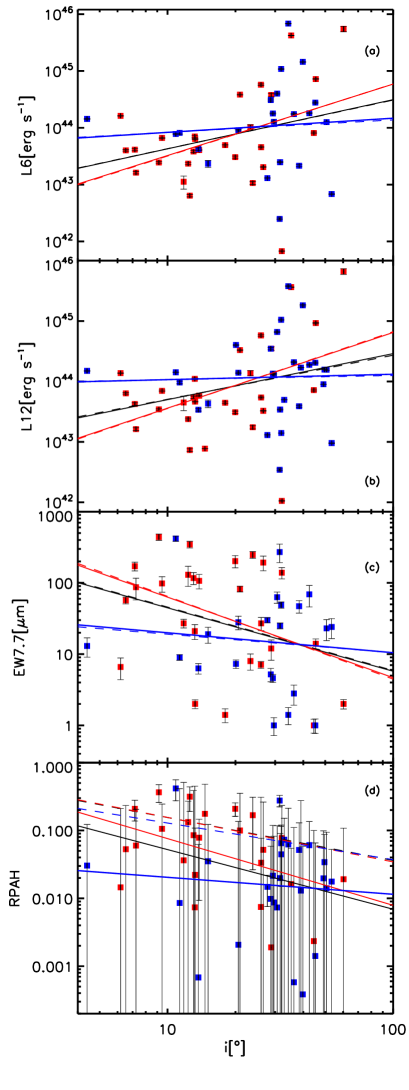
Figure 6: The trends for all objects from the sample: inclination, $i$ vs. L6 (a), L12 (b), EW7.7$\mu$m (c), and RPAH (d). The data colour is the same as in Fig. 4. Black lines are fittings with all data, red lines are for NLS1s only, while blue lines are for BLAGNs only. Full lines are obtained without using uncertainties, while dashed lines are obtained using uncertainties.

Table 7: Fitting results for Fig. 6: A – constant, B – slope, R – Pearson correlaton coefficient and P value (without errors included) and: A_e, B_e and R_e correlaton coefficient (with errors included), for all objects, and for NLS1s and BLAGNs separatelly. As it is shown in the last column, for BLAGNs there are no trends.

	mark	A	B	R	P	Ae	Be	Re	Related?
All	a	42.77$\pm$0.54	0.86$\pm$0.40	0.299	0.036	42.77$\pm$0.56	0.86$\pm$0.41	0.30$\pm$0.13	yes
NLS1s	a	42.25$\pm$0.70	1.26$\pm$0.55	0.414	0.032	42.24$\pm$0.74	1.27$\pm$0.57	0.46$\pm$0.19	yes
BLAGNs	a	43.67$\pm$0.96	0.25$\pm$0.67	0.084	0.710	43.70$\pm$1.00	0.22$\pm$0.69	0.07$\pm$0.22	no
All	b	42.94$\pm$0.48	0.76$\pm$0.35	0.285	0.033	42.97$\pm$0.51	0.73$\pm$0.37	0.28$\pm$0.12	yes
NLS1s	b	42.30$\pm$0.66	1.25$\pm$0.52	0.426	0.024	42.28$\pm$0.69	1.27$\pm$0.54	0.46$\pm$0.18	yes
BLAGNs	b	43.94$\pm$0.79	0.09$\pm$0.54	0.032	0.872	43.96$\pm$0.81	0.07$\pm$0.55	0.03$\pm$0.20	no
All	c	2.54$\pm$0.51	-0.89$\pm$0.38	-0.322	0.025	2.55$\pm$0.53	-0.89$\pm$0.40	-0.34$\pm$0.14	yes
NLS1s	c	2.93$\pm$0.69	-1.13$\pm$0.55	-0.390	0.049	2.97$\pm$0.71	-1.16$\pm$0.56	-0.43$\pm$0.19	yes
BLAGNs	c	1.58$\pm$0.86	-0.28$\pm$0.60	-0.102	0.650	1.54$\pm$0.89	-0.26$\pm$0.62	-0.10$\pm$0.24	no
All	d	-0.40$\pm$0.47	-0.88$\pm$0.34	-0.340	0.013	-0.18$\pm$0.63	-0.63$\pm$0.47	-0.68$\pm$1.20	yes
NLS1s	d	-0.14$\pm$0.54	-0.98$\pm$0.44	-0.420	0.034	-0.15$\pm$1.15	-0.65$\pm$0.97	-0.61$\pm$1.78	yes
BLAGNs	d	-1.44$\pm$0.89	-0.25$\pm$0.60	-0.084	0.678	-0.35$\pm$1.18	-0.54$\pm$0.82	-0.35$\pm$0.78	no

3.2 The correlations for model of dusty hyperboloid shell compared with spectroscopic correlations

In Section 2.1 we calculated the surfaces of hyperbola and dusty disc projections to the plane of the observer (Table 4, Figs. 2 and 3). These projected surfaces in dependence from $i$ are shown in Fig. 7. As one can see from the Table 4 and Fig. 7, for hyperbola part the projection surfaces ($S_{{\rm hyp}}$) grow for inclinations up to $\sim$30$\degree$, and then they decline, while $S_{{\rm ddisc}}$ decrease with the inclination. Their sums, $S_{{\rm hyp\texttt{+}ddisc}}$, also rise for inclinations up to $\sim$30$\degree$, and then they fall. This sum of surfaces (fourth column of Table 4) should be determining the luminosity of the AGN (as the luminosities are additive), in case that the sheltering is not too high.

Figure 7: Projected surfaces (to the plane of observer) of hyperboloid (H), disc (D) and added hyperboloid and disc (H+D) for the data from the Table 4. The sum of hyperboloid and dusty disc surfaces increases up to $\sim$30$\degree$ (vertical line), and then it drops. For hyperboloid, projected surface also rises up to $\sim$30$\degree$, and then decline, while for dusty disc it decreases all the time.

$S_{{\rm hyp\texttt{+}ddisc}}$ increases and then decreases with a turning point around 30$\degree$ (Fig. 7). The trends for $i\leq$30 $\degree$ and $i\geq$30$\degree$ are given in the Fig. 7. That reminds on the spectroscopic relations shown in Fig. 8, where the three correlations from the data from La18 paper are given, FWHM(H$\beta$) vs. the luminosities at 6 and 12 $\mu$m and the luminosity at 5100 Å, (a), (b) and (c), respectively. In La18, it was presented that NLS1s have positive correlations between FWHM(H$\beta$) and aforementioned luminosities, luminosity of broad H$\beta$ line and several MIR coronal lines, while BLAGN do not have, or have weak negative correlations. Also, La18 noticed that RPAH is anticorrelated with FWHM(H$\beta$) for NLS1s (Fig. 5).

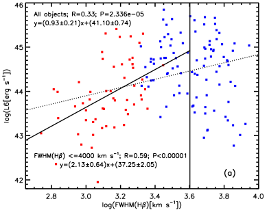
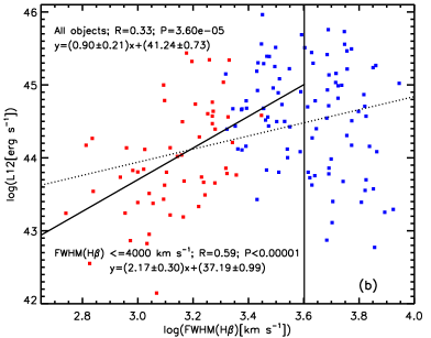
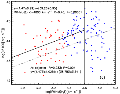
Figure 8: The relations between FWHM(H$\beta$) and L6 (a), FWHM(H$\beta$) and L12 (b) and between FWHM(H$\beta$) and L5100 (c), for the data from La18. The coefficient of correlation (R) and best linear fit are calculated for objects with FWHM(H$\beta$)$<$4000 km s^-1, left from vertical line (fitted with solid line), since for FWHM(H$\beta$)$>$4000 km s^-1 there are no trends, and for all objects (fitted with dotted line). The data colour is the same as in Fig. 4.

Note that in Fig. 8 (a), (b) and (c) we present the trends for total sample (dotted) line), separately from the trends for objects with FWHM(H$\beta$) $\leq$4000 km s^-1 (full line), which is different than the boundary between NLS1s and BLAGNs, FWHM(H$\beta$)=2200 km s^-1 (Rakshit et al., 2017), for the two reasons. Firstly, it looks like the turning point of these datapoints according to free assessment, secondly because the relation in Fig. 4 suggests that FWHM(H$\beta$)=4000 km s^-1 corresponds to 29.72$\degree\sim$30$\degree$ (which is actually also the turning point for Fig. 7). By chance, the correlations are stronger for this boundary. For the FWHM(H$\beta$)–L6, for FWHM(H$\beta$) $\leq$2200 km s^-1, the trend had Pearson correlation R= 0.51; P= 6.19x10^-5, while the correlation for FWHM(H$\beta$) $\leq$4000 km s^-1 is shown in Fig. 8 (a), and it is somewhat stronger. Similarly, for FWHM(H$\beta$) $\leq$2200 km s^-1, the trend of FWHM(H$\beta$)–L12 had Pearson correlation R=0.497; P= 0.00011, while for FWHM(H$\beta$) $\leq$4000 km s^-1the stronger trend is shown in Fig. 8 (b). For the FWHM(H$\beta$)–L5100, for FWHM(H$\beta$) $\leq$2200 km s^-1 we did not find a trend, while the trend for FWHM(H$\beta$) $\leq$4000 km s^-1 is shown in Fig. 8 (c). The rest of the data (FWHM(H$\beta$) $>$4000 km s^-1) does not show significant trends.

In Fig. 9 we show the surfaces of projections (to the plane of the observer) of 4 hyperboloids, two with heights 6.23 pc and two with heights of 40 pc (see the legend), in dependence from $i$. They have $\theta\texttt{=}$ 30, 50, 53 and 60$\degree$. One can notice that the curve shape depends on the angle (steeper rise and shallower drop for smaller angles), but does not depend on the cone height. All curves flatten out around 30-40$\degree$, and afterwards they start decreasing.

Figure 9: Projected surfaces (to the plane of observer) of hyperboloid (H) for various angles $\theta$ and hyperboloid heights h (see the legend). The real H surfaces are divided to certain numbers (see the legend) in order to be presented in the same plot. Some curves break around 30$\degree$, while others break around 40$\degree$.

3.3 Including optical depth

We assume that there is some loss in the MIR radiation due to absorption and scaterring, that for $i\texttt{=}$90$\degree$ the optical depths of hyperboloid and dusty disc are $\tau_{90\degree}^{h}\texttt{=}$2.5 and $\tau_{90\degree}^{d}\texttt{=}$15, respectively (for S19 model), and that the density and the opacity are constant. Here we included the optical depths of hyperboloid and dusty disc in rough approximations. If we define the optical depth, $\tau$ as the height ot the fictive cylinder of the same volume $V$ as cone/dusty disc, and the base $S$ (projection surface), such that $V$/$S\texttt{=}\tau$, then

$$\frac{V}{S_{90,{\rm hyp}}}:\tau_{90\degree}^{h}\texttt{=}\frac{V}{S_{i,{\rm hyp}}}:\tau_{i}^{h}\Rightarrow\frac{\tau_{i}^{h}}{S_{90,{\rm hyp}}}\texttt{=}\frac{\tau_{90}^{h}}{S_{i,{\rm hyp}}},$$ (9)

therefore the optical depths of hyperboloid and dusty disc can be approximated as:

$$\tau_{i}^{h}\texttt{=}\frac{S_{90\degree,{\rm hyp}}}{S_{i,{\rm hyp}}}\times\tau_{90\degree}^{h}$$ (10)

and

$$\tau_{i}^{d}\texttt{=}\frac{S_{90\degree,{\rm ddisc}}}{S_{i,{\rm ddisc}}}\times\tau_{90\degree}^{d}.$$ (11)

The dependence of $\tau$ from $i$ is given in Fig. 10. Including $\tau$, the intensity of the source is approximately estimated with formulas I${}_{h}\sim$ e${}^{-\tau_{{\rm hyp}}}$ and I${}_{d}\sim$ e${}^{-\tau_{{\rm ddisc}}}$, see Fig 11. Here, the peak of intensity is again around 30$\degree$. The curve for a cone (Fig 11) is somewhat steeper than the one in Fig. 7, even if $\tau\texttt{=}\tau$/2 would be taken. Also, the curves for cones for other (larger) angles $\theta$ are also getting somewhat steeper when the average optical thickness is included. However, these approximations are rough and the more detailed approach is needed, such as radiative transfer.

Figure 10: Average estimation of $\tau$ for various inclinations for S19 model, for hyperboloid (H), disc (D) and hyperboloid + disc (H+D).

Figure 11: Average estimation of I$\sim$ e^-τ for various inclinations of disc (D), hyperboloid (H), and disc + hyperboloid (H+D), for S19 model. The vertical line marks $i\texttt{=}$30$\degree$, where the break for cone occurs.

3.4 Comparison with observational datasets

As the correlations that could be found for some sample depend on the characteristics of the objects from that sample (as the range of the cosmological redshift, continuum luminosities, M_BH, broad lines width. etc.), we checked if luminosities-FWHM(H$\beta$) correlations can be found for samples that significantly differ from the dataset from this work. The characteristics of these NLS1 samples and their correlations are given in the Table 8.

Having in mind other datasets and measurements of FWHM(H$\beta$) vs. various luminosities, we noticed that the luminosities are not necessarilly in the same trend with FWHM(H$\beta$). For example as e.g. Fig. 12 from Zhou et al. (2006) (0$<z<$0.8; 40$<$log(LH$\beta$)$<$44), where FWHM(H$\beta$) and FWHM(H$\alpha$) vs. their luminosities are given for NLS1s, objects are confined under the guiding line and their trends are only R=0.29 and R=0.34, respectively. They explain this by the existence of upper limits in the accretion rate in units of the Eddington rate. On the other hand, Véron-Cetty et al. (2001) obtained stronger correlation for FWHM(H$\beta$) and its luminosity: 0.76, while this relation covers both NLS1 objects with z$<$0.1, 40$<$log(LH$\beta$)$<$44 and BLAGNs with 41$<$log(LH$\beta$)$<$46.

Table 8: The characteristics and chosen correlation coefficients for NLS1 data samples from Section 3.4.

Sample	z	log(Lumin.) [erg s-1]	size	FWHM(H$\beta$)-L(H$\beta$)	FWHM(H$\beta$)-X lumin.	FWHM(H$\beta$)-L5100
this work	z$<$0.3	42$<$L5100<46	56	NA	NA	NA
Zhou et al. (2006)	0$<$z$<$0.8	40$<$log(LH$\beta$)$<$44	2000	0.29	NA	NA
		41$<$L5100<46
Véron-Cetty et al. (2001)	z$<$0.1	40$<$log(LH$\beta$)$<$46	64	0.76	NA	NA
Kovačević et al. (2010)	z$<$0.7	43$<$log(L5100)$<$47	92	0.39	NA	0.33
FWHM(H$\beta$)$<$2200 km s-1		40$<$log(LH$\beta$)$<$44)		P=0.00013		P=0.0015
Rakshit et al. (2017)	z$<$0.8	42$<$log(L5100)$<$45	11101	NA	NA	no trend
Bianchi (2009)	z$<$0.4	41$<$Hard X lum. $<$45	23	NA	Hard: 0.37; Hard and	NA
					soft lum. ratio: -0.64
Lakićević et al. (2018)	z$<$0.7	42$<$log(L5100)$<$46	64	0.734	0.471	no trend
				P=7.9$\times$10-5	P=0.004

Regarding the dataset from Kovačević et al. (2010) ($z<0.7$; 43$<$log(L5100)$<$47; 40$<$log(LH$\beta$)$<$44), the FWHM(H$\beta$)–L5100 relation from their measurements and trend for FWHM(H$\beta$)$\leq$4000 km s^-1 are given in Fig. 12. Similarly as before, the correlations are higher for FWHM(H$\beta$)$\leq$4000 km s^-1 than for NLS1s only (for FWHM(H$\beta$)$\leq$ 2200 km s^-1, R=0.326, P=0.0015). Analyzing the same sample, Popović & Kovačević (2011) noticed high FWHM(H$\beta$)–L5100 correlation for the objects with high starburst contribution, see their Fig. 7, left.

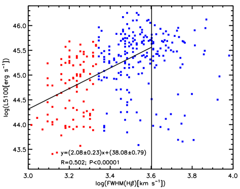
Figure 12: A relation FWHM(H$\beta$)–L5100 made from the data from paper Kovačević et al. (2010), for the objects where FWHM(H$\beta$)$<$4000 km s^-1. The data colour is the same as in Fig. 4.

The FWHM(H$\beta$)–L5100 relation for NLS1s from Rakshit et al. (2017) ($z<0.8$; 42$<$log(L5100)$<$45) is presented in Fig 13. Here NLS1s do not show the trend with FWHM(H$\beta$) (coefficient R=0.142; P$<$10^-6), but they are approximatelly settled below the line y=2.08x + 38.2. In this sample they included only objects with FWHM(H$\beta$)$<$2200 km s^-1.

Figure 13: FWHM(H$\beta$)–L5100 plot, made from the catalogue of NLS1s in Rakshit et al. (2017).

A FWHM(H$\beta$) vs. X-ray luminosity plot, described in La18, can be seen in Bianchi (2009), in their Fig. 2. X-ray luminosity–FWHM(H$\beta$) correlation exists for NLS1s only (same like for MIR and optical luminosities in other datasets). The most of objects in the sample have $z\lesssim 0.4$.

4 Discussion

Zhang & Wu (2002) used disc-like BLR model, calculating M_BH from the stellar velocity despersion (as this method is not too dependent on the BLR inclination), to obtain the inclination of the BLR, $i$. Zhang & Wu (2002) noticed that $i$ is dependent on the FWHM(H$\beta$) (see their Fig. 3 and Section 3.1 in this paper). This encourages us to connect aforementioned correlations (FWHM(H$\beta$)–luminosities) with the inclination and perhaps with spectral properties of NLS1s and BLAGNs (discussed in Section 4.1). In the Section 4.2 we consider the possible connection of FWHM(H$\beta$)–luminosities correlations with the cone model of AGNs.

4.1 NLS1s, BLAGNs, inclination and spectroscopic correlations

The calculation of the inclination angle of BLR using Equation 1 predicts the higher FWHM of broad lines for higher inclinations (Fig. 4), as the projections of the velocities of the matter around BHs to the direction to the observer are higher for objects with higher $i$. Therefore, NLS1s could be the same objects as BLAGNs, but observed under the lower inclination (Nagao et al., 2000; Zhang & Wu, 2002). Zhang & Wu (2002) found that $i$ are significantly higher for BLAGNs than for NLS1s and that $i$ for NLS1s rarely exceeds 30$\degree$.

Various datasets such as La18, Kovačević et al. (2010); Véron-Cetty et al. (2001); Zhou et al. (2006); Bianchi (2009); Järvelä et al. (2015); Lakićević et al. (2018) show FWHM(H$\beta$)-luminosities correlations for NLS1s (Section 3.4, Table 8). These various datasets are similar in the redshift and luminosity range, which means that these correlations exist for that type of objects, and that they are not accidentally biased by some sample choosing.

Lower luminosities for NLS1s than for BLAGNs are shown in La18 and references therein. In Fig. 8, it seems that FWHM-luminosities trends do not exist only for NLS1s (FWHM(H$\beta$) $\lesssim$2200 km s^-1 and $i\lesssim$15$\degree$ – according to relation in Fig. 4), like it was thought in La18, but up to FWHM(H$\beta$) $\lesssim$4000 km s^-1, where $i\lesssim$30-40$\degree$; as relations for FWHM(H$\beta$) $\lesssim$4000 km s^-1 are stronger than only for NLS1s. Similar is with FWHM(H$\beta$)-L5100 relation for Popović & Kovačević (2011) dataset. That could mean that these correlations may not exist due to NLS1-BLAGN differences, but as a consequence of some other reason, such as possibly the geometry and $i$. As it can be seen in spectroscopic measurements in Fig. 6 a and b, the MIR luminosities have weak trend (R=0.28-0.30) with calculated $i$ for all data. Since FWHM(H$\beta$) increases with the inclination (Fig. 4), and since FWHM(H$\beta$) is correlated with luminosities only for objects with FWHM(H$\beta$)$\lesssim$4000 km s^-1 (Fig. 8), which corresponds to the $i\sim$30$\degree$ (Fig. 4), the trend $i$–luminosities is expected to exist for objects with $i\lesssim 30-40\degree$ in particular. However, this is not the case; the trends in Fig. 6 become insignificant if the objects with $i>$ 30-40$\degree$ are excluded from the fit. If the objects with $i>$40$\degree$ are excluded, the correlation parameters for L6 are: P=0.23; R=0.61 and for L12 they are: R=0.23; P=0.12. The correlation may be lost because of small dataset, as the poor correlation could be lost if number of data is lower.

The separation of objects to the ones with FWHM(H$\beta$)$\lesssim$4000 km s^-1 and others that have FWHM(H$\beta$)$\gtrsim$4000 km s^-1 might have the similarity with the separation to Populations A and B from Sulentic et al. (2000, 2009). According to Sulentic et al. (2009) 50-60% of of radio quiet sources have FWHM(H$\beta$)$<$4000 km s^-1, show blueshift and asymmetry of high ionisation lines, strong FeII emission and a soft X-ray excess (so called Population A); while almost all radio loud sources have FWHM(H$\beta$)$>$4000 km s^-1, weak FeII emission, and lack of a soft X-ray excess (Population B).

Although NLS1s and BLAGNs could have the same structure (Zhang & Wu, 2002; Decarli et al., 2008), some authors claim that NLS1s may be in early stage of evolution compared to BLAGNs (Mathur, 2001), with lighter M_BHs (Peterson, McHardy & Wilkes, 2000; Komossa & Xu, 2007). In Fig. 5, similarly as in Fig. 6 d and e ($i$-EW7.7 and $i$-RPAH), the known FWHM(H$\beta$)-RPAH anticorrelation is shown (present only for the NLS1s; La18). PAHs are more pronounced for the low FWHMs and inclination angles. RPAH is also known to be anticorrelated with M_BH and possibly destroyed close to AGN (e.g. Lakićević et al., 2017, and references therein), thus the reason for higher RPAH in NLS1s (small $i$) can be lighter M_BH in NLS1s. NLS1s have more dusty spiral arms and bars (Deo et al., 2006), where PAHs may be located (Siebenmorgen et al., 2004), since PAHs are star formation tracer (Peeters et al., 2004; Shipley et al., 2016). Star formation occurs in spiral arms (Baade, 1963), and spiral arms and bars may be more visible because of low $i$. Afterwards, star formation may drive mass inflow into AGNs, supporting BH growth (Alexander & Hickox, 2012) and NLS1s have higher accretion rate. There may be some connection between the dusty cone geometry and the starbursts, so that the starburst are more apparent for low inclinations.

In order to check if star formation rate (SFR) is stronger for lower $i$ (since there RPAH is higher), we used the equation from Sargsyan & Weedman (2009):

$$log\left[SFR\left(PAH\right)\right]\texttt{=}log\left[\nu L_{\nu}\left(7.7\mu m\right)\right]\texttt{-}42.57\pm 0.2,$$ (12)

to find SFR. There, flux density at the peak of the 7.7 $\mu$m feature is used to find luminosity at 7.7 $\mu$m, $\nu L_{\nu}$(7.7$\mu$m). In Fig. 14 we showed $i$ vs $SFR\left(PAH\right)$ estimated from the Equation 12. The fitting results without errors included and the ones accounted for the errors are given in the Table 9 and the best fits are shown in the Fig. 14. As one can see from Fig. 14, there is no obvious correlation between $i$ and SFR, although the sample is small. On the other hand, SFR depends on PAH luminosity, which is different parameter than the PAH contribution in the spectra (RPAH), that is found to be stronger at low inclinations (Fig. 6 c, d).

Figure 14: Inclination–SFR plot for sample from this work. The full line is fit without uncertainties, while the dashed line is fit with included errors.

Table 9: Fitting results for Fig. 14: A – constant, B – slope, R – Pearson correlaton coefficient and P value (without errors included) and: A_e, B_e and R_e correlaton coefficient (with errors included), for all objects. There is no correlation.

	A	B	R	P	Ae	Be	Re	Related?
All	0.33$\pm$0.54	-0.16$\pm$0.40	-0.06	0.69	0.49$\pm$0.80	-0.09$\pm$0.57	-0.03$\pm$0.21	no

4.2 FWHM(H$\beta$)-luminosity correlations and cone model of AGN

Firstly, we assumed a model consisting of the hyperboloid shell and a thin dusty disc, from S19. Seeing an AGN in different angles, the AGN luminosity should be dependent on the surface of the object that the observer is seeing (due to dust obscuration). The two observed surfaces are added and the total surface, $S_{{\rm hyp\texttt{+}ddisc}}$ is obtained. Both $S_{{\rm hyp\texttt{+}ddisc}}$ and $S_{{\rm hyp}}$ increase up to 30$\degree$, and then they drop (Fig. 7), which resembles to the turning point in relations in Fig. 8, but with $\sim$10 times lower slope. However, when the optical depth, $\tau$, in shape $I\sim e^{-\tau}$ is included, the slope for the cone becomes somewhat steeper (Fig. 11). This break that happens both in Fig. 7 and for real data (Fig. 8) offers one possible explanation for FWHM(H$\beta$)–luminosities relations.

Similar results are obtained when the cones of different dimensions and $\theta$ are considered. For all angles $\theta$, thicknesses and heights, the break is always at 30-40$\degree$, while the slopes depend on $\theta$ (Fig. 9). The smaller angle $\theta$ is, the higher dependence of projection surface to the plane of the observer from inclination (steeper slope) is for $i\lesssim$30$\degree$ and the shallower slope is for $i\gtrsim$30$\degree$.

Another possible explanation for FWHM(H$\beta$)–luminosities relations is that perhaps low-mass AGNs (AGNs with low luminosities) are not seen in large angles, but only in small angles, since these systems are not confined enough, they are younger objects, their dust may be more likely located in cones and they may be hard to notice at higher $i$ because of the obscuration (Popović et al., 2018). That is one possible selection effect, but we are not aware if there are some other selections that could possibly hide some objects. Together or separately, dependence of luminosities on the observed object surface and/or a lack of light M_BHs for large $i$ may be cause of mentioned correlations.

It could be expected that the decrease of the luminosity for higher angles ($\gtrsim$30$\degree$) may be also due the observing through the dusty cone or torus or catching more galactic noise. Also, the disagreement between Figs. 7 and 11 with Fig. 8 for $i\gtrsim$30$\degree$, FWHM(H$\beta$)$\gtrsim$4000 km s^-1 (in Fig. 8 the trends are missing) may be due to galactic noise and irregularities.

Luminosities of lines and continuum at different wavelengths are usually strongly correlated in the datasets of various AGNs, and that could offer the explanation for mentioned luminosity trends. The optical luminosities (L5100) should behave similar as MIR luminosities (L6 and L12). Afterall, MIR cones are spread to the much larger distances ($\sim$ 100 pc), while optical data (L5100 and FWHM(H$\beta$)) come from the BLR which has a size of $\sim$10^-2 pc (Hawkins, 2007). The size of MIR cones could be a measurement of its AGN power and probably M_BH.

Finally, L5100–FWHM(H$\beta$) correlation could be connected with starbursts, as it was suggested by Popović & Kovačević (2011), who found strong relation (R=0.8), for starburst dominated objects (see their Fig. 7). However, starburst dominated objects are often NLS1s, and therefore geometry could still be the explanation. It is important to do further studies.

5 Conclusions

We explored the influence of calculated inclination ($i$) to the luminosities of the Type 1 AGNs using 1) a sample model of dusty cone shells, and/or 2) the selection effect by the BH mass. Inclinations of AGNs are found from optical data. Since $i$ and FWHM(H$\beta$) are correlated and since FWHM(H$\beta$) have the trends with optical, MIR and X-ray luminosities, $i$ should also have trends with these luminosities for $i\lesssim$30-40$\degree$. Here, it is noticed that FWHM(H$\beta$)-luminosities correlations cover broader range, FWHM(H$\beta$)$\lesssim$4000 km s^-1 than it was previously thought (FWHM(H$\beta$)$<$2200 km s^-1; La18).

The inclination obtained from spectroscopic data vs. luminosity trends for AGNs are similar with the inclination–S trend (S is surface of the observed cone model), because S should determine luminosity. Both of these relations break around 30$\degree$. When the optical depths are included, the slope inclination–S is deeper. That could mean that the dusty cone geometry is the cause of FWHM(H$\beta$)-luminosities correlations.

The alternative explanation for inclination–luminosity relations may be the selection effect by M_BH (low-luminosity AGNs with lighter M_BH may be less confined, material spread in cones, and these objects may not be seen at large FWHMs).

From our investigations we can point out following:

• Possibly, $i$-luminosities and $i$–RPAH (FWHM(H$\beta$)-luminosities and FWHM(H$\beta$)–RPAH) relations for FWHM(H$\beta$)$\lesssim$4000 km s^-1 are consequence of the dusty cone geometry of an AGN and the angle of view.

• Beside differencies in BH mass, (NLS1s have lighter black hole mass than BLAGNs), inclination of the dusty conical AGN geometry may also be the cause of differences between NLS1s and BLAGNs, where NLS1s may be seen in lower inclination angles.

• Finding the inclinations and the making AGN models may help in understanding Type 1 and 2 AGNs and possibility of unification scheme.

Data Availability

The data underlying this article are available in the article and in its online supplementary material. The data underlying this article are compiled from the literature, calculated from the literature data or measured from the spectra that are available to the public (CASSIS database).

References

- Afanasiev et al. (2019) Afanasiev, V. L., Popović, L. Č. & Shapovalova, A. I. 2019, MNRAS, 482, 4985
- Alexander & Hickox (2012) Alexander, D. M., & Hickox, R. C. 2012, New Astron. Rev., 56, 93
- Alonso-Herrero et al. (2018) Alonso-Herrero, A., Pereira-Santaella, M., García-Burillo, S., et al. 2018, ApJ, 859, 144
- Alonso-Herrero et al. (2021) Alonso-Herrero, A. et al. 2021, A&A, 652, 99
- Antonucci (1993) Antonucci, R. 1993, ARA&A, 31, 473
- Asmus (2019) Asmus, D. 2019, MNRAS, 489, 2177
- Baade (1963) Baade, W. 1963, Evolution of stars and Galaxies (Cambridge: Harvard Univ.), p 63
- Bae & Woo (2016) Bae, Hyun-Jin & Woo, Jong-Hak 2016, ApJ, 828, 97
- Baldi et al. (2016) Baldi, R. D., Capetti, A., Robinson, A., et al. 2016, MNRAS, 458, 69
- Bellovary et al. (2014) Bellovary. J. M., Holley-Bockelmann, K., Gültekin, K., et al. 2014, MNRAS, 445, 2667
- Bentz et al. (2013) Bentz, M. C., Denney, K. D., Grier, C. J. et al. 2013, ApJ, 767, 149
- Berton et al. (2015) Berton, M., Foschini, L., Ciroi, S., et al. 2015, A&A, 578, 28
- Bian et al. (2010) Bian, W.-H., Huang, K., Hu, C., Zhang, L., Yuan, Q.-R., Huang, K.-L., & Wang, J.-M. 2010, 718, 460
- Bianchi (2009) Bianchi, S., Bonilla, N. F., Guainazzi, M., Matt, G. & Ponti, G. 2009, A&A, 501, 915
- Boller et al. (2001) Boller, Th. 2001, AIP Conference Proceedings 599, 25
- Boroson & Green (1992) Boroson, T. A. & Green, R. F. 1992, ApJS, 80, 109
- Buat et al. (2021) Buat, V. et al. 2021, arXiv:2108.07684
- Decarli et al. (2008) Decarli, R., Dotti, M., Fontana, M. & Haardt, F. 2008, MNRAS, 386, L15
- Collin et al. (2006) Collin, S., Kawaguchi, T., Peterson, B. M., & Vestergaard, M. 2006, A&A, 456, 75
- Deo et al. (2006) Deo, R. P., Crenshaw, D. M., & Kraemer, S. B. 2006, AJ, 132, 346
- Gallimore et al. (2016) Gallimore, J. F., Elitzur, M., Maiolino R. et al. 2016, ApJ, 829, 7
- García-Burrilo et al. (2014) García-Burillo, S., Combes, F., Usero, A. et al. 2014, A&A, 567, A125
- Gonçalves et al. (1999) Gonçalves, A. C., Véron, P. & Véron-Cetty M.-P. 1999, A&A, 341, 662
- Goodrich (1989) Goodrich, R. W. 1989, ApJ, 342, 224
- GRAVITY Collaboration et al. (2018) GRAVITY Collaboration, Sturm, E., Dexter, J. et al. 2018, Nature, 563, 657-660
- Grupe et al. (1999) Grupe, D., Beuermann, K., Mannheim, K., & Thomas, H.-C. 1999, A&A, 350, 805
- Hawkins (2007) Hawkins, M. R. S. 2007, A&A, 462, 581
- Hernán-Caballero et al (2015) Hernán-Caballero, A., Alonso-Herrero, A., Hatziminaoglou, E. et al. 2015, ApJ, 803, 109
- Hönig (2019) Hönig, S. F. 2019, ApJ, 884, 171
- Järvelä et al. (2015) Järvelä, E. Lähteenmäki, A., & León-Tavares, J. 2015, A&A, 573, A76
- Järvelä et al. (2017) Järvelä, E. Lähteenmäki, A., Lietzen, H., Poudel, A. Heinämäki, P., & Einasto, M. 2017, A&A, 606, 9
- Jarvis & McLure (2006) Jarvis, M. J. & McLure, R. J. 2006, MNRAS, 369, 182
- Jin et al. (2012a) Jin, C., Ward, M., & Done, C. 2012a, MNRAS, 422, 3268
- Jin et al. (2012b) Jin, C., Ward, M., & Done, C. 2012b, MNRAS, 425, 907
- Kelly (2007) Kelly, B. C. 2007, ApJ, 665, 1489
- Komossa & Xu (2007) Komossa, S. & Xu, D., 2007, ApJ, 667, L33
- Kovačević et al. (2010) Kovačević, J., Popović, L. Č., Dimitrijević, M. S. 2010, ApJS, 189, 15
- Klimek et al. (2004) Klimek, E. S., Gaskell, C. M., & Hedrick, C. H. 2004, ApJ, 609, 69
- Lakićević et al. (2017) Lakićević, M., Kovačević-Dojčinović, J., Popović, L. Č. 2017, MNRAS, 472, 334
- Lakićević et al. (2018) Lakićević, M., Popović, L. Č., Kovačević-Dojčinović, J. 2018, MNRAS, 478, 4068
- Lebouteiller et al. (2011) Lebouteiller, V., Barry, D. J., Spoon, H. W. W., Bernard-Salas, J., Sloan, G. C., Houck, J. R., & Weedman, D. 2011, ApJS, 196, 8
- Lebouteiller et al. (2015) Lebouteiller, V., Barry, D. J., Goes, C., Sloan, G. C., Spoon, H. W. W., Weedman, D. W., Bernard-Salas, J., Houck, J. R. 2015, ApJS, 218, 21
- Liu et al. (2016) Liu X., Yang P., Supriyanto R. & Zhang Z. 2016, IJAA, 6, 166
- Marin et al. (2015) Marin, F., Goosmann, R. W., & Gaskell, C. M. 2015, A&A, 577, A66
- Markowitz et al. (2014) Markowitz, A. G., Krumpe, M., Nikutta, R. 2014, MNRAS, 436, 1403
- Marinello et al. (2016) Marinello, M., Rodríguez-Ardila, A., Garcia-Rissmann, A., Sigut, T. A. A. & Pradhan, A. K. 2016, ApJ, 820, 116
- Marziani et al. (1993) Marziani, P., Sulentic, J. W., Calvani, M., Perez, E., Moles, M., & Penston, M. V. 1993, ApJ, 410, 56
- Mathur (2000) Mathur, S. 2000, New Astron. Rev., 44, 469
- Mathur (2001) Mathur, S., Kuraszkiewicz, J., & Czerny, B. 2001, New A, 6, 321
- Nagao et al. (2000) Nagao, T., Taniguchi, Y., & Murayama, T. 2000, AJ, 119, 2605
- Nikołajuk et al. (2009) Nikołajuk, M., Czerny, B. & Gurynowicz, P. 2009, MNRAS, 394, 2141
- Osterbrock & Pogge (1985) Osterbrock, D. E., & Pogge, R. W. 1985, ApJ, 297, 166
- Peeters et al. (2004) Peeters, E., Spoon, H. W. W. & Tielens, A. G. G. M. 2004, ApJ, 613, 986
- Peterson, McHardy & Wilkes (2000) Peterson B. M., McHardy I. M., Wilkes B. J., 2000, New Astron. Rev., 44, 491
- Popović et al. (2018) Popović, L. Č., Afanasiev, V. L., & Shapovalova, A. I. 2018, PoS (NLS1-2018) 001
- Popović & Kovačević (2011) Popović, L. Č. & Kovačević, J. 2011, ApJ, 738, 68
- Rakshit et al. (2017) Rakshit, S., Stalin, C. S., Chand, H. & Zhang, X.-G. 2017, ApJS, 229, 39R
- Rakshit & Stalin (2017) Rakshit, S. & Stalin, C. S. 2017, ApJ, 842, 96
- Sani et al. (2010) Sani, E., Lutz, D., Risaliti, G., Netzer, H., Gallo, L. C., Trakhtenbrot, B., Sturm, E. & Boller, T. 2010, MNRAS, 403, 1246
- Sargsyan & Weedman (2009) Sargsyan, L. A. & Weedman, D. W. 2009, ApJ, 701, 1398
- Schmidt et al. (2016) Schmidt, E. O., Ferreiro, D., Vega Neme, L & Oio, G. A. 2016, A&A, 596, 95
- Shapovalova et al. (2012) Shapovalova, A. I., Popović, L. Č., Burenkov, A. N. et al. 2012, ApJS, 202, 10
- Shipley et al. (2016) Shipley, H. V., Papovich, C., Rieke, G. H., Brown, M. J. I. & Moustakas, J. 2016, ApJ, 818, 1
- Siebenmorgen et al. (2004) Siebenmorgen, R., Krügel, E., & Spoon, H. W. W. 2004, A&A, 14, 123
- Stalevski et al. (2019) Stalevski, M., Tristram, K. R. W. & Asmus, D. 2019, MNRAS, 484, 3334
- Sulentic et al. (2000) Sulentic, J. W., Marziani, P. & Dultzin-Hacyan, D. 2000, ARA&A, 38, 521
- Sulentic et al. (2002) Sulentic, J. W., Marziani, P., Zamanov, R., Bachev, R., Calvani, M., & Dultzin-Hacyan, D. 2002, ApJ, 566, L71
- Sulentic et al. (2009) Sulentic, J. W., Marziani, P. & Zamfir, S., 2009, New A Rev., 53, 198
- Toba et al. (2021) Toba, Y. et al., 2021, ApJ, 912, 91
- Tristram & Schartmann (2011) Tristram, K. R. W. & Schartmann M., 2011, A&A, 531, 99
- Urru & Padovani (1995) Urru, C. M. & Padovani, P., 1995, PASP, 107, 803
- Véron-Cetty et al. (2001) Véron-Cetty, M. P., Véron, P., & Gonc¸alves, A. C., 2001, A&A, 372, 730
- Véron-Cetty et al. (2010) Véron-Cetty, M. P. & Véron, P. 2010, A&A, 518, 10
- Yang (2018) Yang, H. Yuan, W, Yao, S. et al. 2018, MNRAS, 477, 5127
- Zhang et al. (2013) Zhang, K., Wang, T.-G. Yan, L., & Dong, X.-B. 2013, ApJ, 768, 22
- Zhang & Wu (2002) Zhang, T.-Z. & Wu, X.-B., 2002, Chin. J. AA, 2, 487
- Zhou et al. (2006) Zhou, H., Wang, T., Yuan, W., Lu, H., Dong, X., Wang, J., & Lu, Y. 2006, ApJS, 166, 128