The CN2HDM

Abstract

We present the CP-violating Next-to-2-Higgs-Doublet Model (CN2HDM) which is based on the extension of the CP-violating 2-Higgs-Doublet-Model (C2HDM) by a complex singlet field that obeys a discrete $\mathbb{Z}_{2}$ symmetry. The model thus features not only CP violation required for successful electroweak baryogenesis but also a Dark Matter (DM) candidate. The model has an extended Higgs sector with four CP-mixing visible neutral Higgs bosons, a DM candidate and a pair of oppositely charged Higgs bosons. The possibility of singlet and CP-odd admixtures to the observed Higgs boson in addition to the large number of visible scalar particles leads to an interesting Higgs phenomenology. We find that the model can easily provide 100% of the DM relic density and investigate interesting LHC and DM observables within the model. We provide all the tools necessary to study the CN2HDM in detail and point out future research directions for this interesting benchmark model that can address some of the most pressing open questions of the Standard Model.

1 Introduction

The discovery of a Higgs boson by the ATLAS [1] and CMS [2] collaborations that behaves very similar to the expectations within the Standard Model (SM) has undoubtedly been the founding achievement of the LHC runs so far. Contrarily, searches for physics beyond the Standard Model (BSM) have come up empty so far, but remain promising avenues to explore. BSM physics is motivated by a number of questions unanswered by the SM, including those on how to explain Dark Matter (DM) and Dark Energy that make up $95\%$ [3, 4, 5] of the physical composition of our universe or how the observed baryon-antibaryon asymmetry [6] can be established. A dynamical mechanism for the generation of the asymmetry is provided by electroweak baryogenesis (EWBG) [7, 8, 9, 10, 11, 12, 13, 14, 15], which requires the three Sakharov conditions to be fulfilled [16]. Among these is the necessity of sufficiently large CP violation which requires additional sources of CP violation beyond the SM.

There is no current precondition to suggest the form that DM should take, whether it be made up of axions, weakly interactive massive particles (WIMPs), or primordial black holes, to name only a few. It is not hard to construct extensions of the SM Higgs sector that can account for the entire DM relic density of the universe through WIMPs. This can be achieved e.g. by adding a neutral real or complex singlet field [17, 18, 19]. Another way is the addition of a second $SU(2)_{L}$ doublet of hypercharge $Y=\pm 1$, which keeps the electroweak precision parameter $\rho=1$ as in the SM [20, 21] and — with its two complex Higgs doublets — reflects the Higgs sector that is the basis for supersymmetry. This extension of the SM Higgs sector gives rise to variations of the 2-Higgs Doublet Model (2HDM) [20, 22], classified by the manner in which the Higgs doublets couple to the fermions. Dark Matter can arise from 2HDMs in various ways, for example in the inert 2HDM [23, 24, 25, 26, 27, 28, 29, 30, 31, 32, 33] where one of the two Higgs doublets is inert, i.e. it does not obtain a vacuum expectation value and hence provides a scalar DM candidate.

CP violation can be induced in the Higgs sector of the 2HDM, without the addition of new fermions, by constructing a 2HDM potential with a softly broken $\mathbb{Z}_{2}$ symmetry with two complex parameters, $\lambda_{5}$ and $m_{12}^{2}$ [34, 35, 36, 37, 38, 39, 40, 41, 42, 43, 44, 45, 46, 47]. Besides CP violation, another salient element for successful EWBG is the interplay between the Higgs mass spectrum and the self-interactions of the Higgs bosons participating in the electroweak phase transition (EWPT). Therefore, a major goal of the upcoming high-luminosity Large Hadron Collider (LHC) is the measurement of the Higgs self-couplings, which is a non-trivial task and requires large di-Higgs cross sections stemming from resonant production of heavy Higgs bosons. The 2HDM becomes increasingly constrained with respect to these collider processes. Additionally, in its type II version it only allows for a heavy Higgs spectrum. This is different in the Next-to-2HDM (N2HDM) [48, 49, 50].

In the N2HDM, an additional real singlet field is added to the two Higgs doublets. The N2HDM is invariant under two $\mathbb{Z}_{2}$ symmetries and, depending on the way in which they are spontaneously broken, the model yields different dark phases with different numbers of DM candidates (or none at all) [51]. Furthermore, the Higgs mass eigenstates get some admixture from the singlet field so that light Higgs states are still allowed in the spectrum that have escaped discovery so far. This implies an interesting LHC phenomenology [50, 52, 51, 53] including the possibility of resonant Higgs production with subsequent decays into Higgs pair final states and even Higgs-to-Higgs cascade decays. The extended Higgs sector can also allow for a strong first order EWPT [54, 55, 56] that is required for EWBG [13, 15]. Thus, the N2HDM can be built up such that it can address some of the most pressing open questions of the SM and additionally provide an interesting landscape for LHC phenomenology. However, while the N2HDM can accommodate DM and realise a first order EWPT, it is defined to be CP-conserving and thus EWBG cannot be realised.

In this work, we present an extension of the N2HDM that addresses this limitation: the CP-violating N2HDM (CN2HDM). It not only incorporates CP violation into its Higgs potential but also contains a DM candidate on top of the particle content of the N2HDM. To achieve this, the model adds a complex singlet field — instead of the real singlet field of the N2HDM — with the $\mathbb{Z}_{2}$ spontaneously broken for the real part, but unbroken for the imaginary component which becomes the DM candidate. At the same time, the real CP-even parts of the doublet and the real singlet field have non-vanishing vacuum expectation values. This construction gives rise to four neutral visible Higgs bosons, a pair of visible oppositely charged Higgs bosons and one DM candidate, allowing for an extremely rich phenomenology. We impose on our model both collider and DM constraints, as well as the constraints stemming from the measurements of the electric dipole moments that are relevant for CP violation. We subsequently investigate — with viable parameter points fulfilling all the imposed constraints — the CN2HDM DM observables and its phenomenology at the LHC. The aim of our paper is the introduction of an interesting benchmark model that features an extended Higgs sector with singlet admixture that is able to address two pressing unsolved questions of contemporary particle physics, the DM candidate and the matter-antimatter asymmetry puzzles. Being a non-supersymmetric model it allows for more freedom in its parameter space and comes along with an interesting LHC phenomenology that can be tested at present and future LHC runs as well as future $e^{+}e^{-}$ colliders.

The outline of our paper is as follows. In Sec. 2 we introduce the CN2HDM with its field content and set up our notation. In the subsequent numerical analysis in Sec. 3, we present the constraints applied and the details of the parameter scan performed. For the latter, we implemented our model in ScannerS [57, 58, 50, 59] and furthermore provide a new Fortran code, CN2HDM_HDECAY, for the computation of the decay widths and branching ratios including state-of-the-art higher-order corrections. We then discuss the interplay of DM constraints and DM observables in our model in Sec. 4 before we move on to the investigation of the CN2HDM Higgs boson phenomenology at the LHC both in the type I and type II versions of the model in Sec. 5. We summarise the findings of our analysis in the conclusion and give an outlook for future directions. In the Appendix, we present auxiliary material, including information on the mixing matrix and physical parameter relations.

2 Model Introduction

The starting point of our CN2HDM model is the N2HDM [48, 49, 50] that we adapt such that it includes both a DM candidate and CP violation. The CN2HDM Higgs sector hence consists of the SM extended by a complex $SU(2)_{L}$ doublet with hypercharge $Y=1$, and a complex $U(1)_{Y}$ singlet with $Y=0$. The potential has two $\mathbb{Z}_{2}$ symmetries: $\Phi_{1,S}\to\Phi_{1,S},\Phi_{2}\to-\Phi_{2}$ is softly broken by $m_{12}^{2}$, while $\Phi_{1,2}\to\Phi_{1,2},\Phi_{S}\to-\Phi_{S}$ remains unbroken in the scalar potential. The potential is given by

$$V = m_{11}^{2}\Phi_{1}^{\dagger}\Phi_{1}+m_{22}^{2}\Phi_{2}^{\dagger}\Phi_{2}+\frac{\lambda_{1}}{2}\left(\Phi_{1}^{\dagger}\Phi_{1}\right)^{2}+\frac{\lambda_{2}}{2}\left(\Phi_{2}^{\dagger}\Phi_{2}\right)^{\dagger}+\lambda_{3}\Phi_{1}^{\dagger}\Phi_{1}\Phi_{2}^{\dagger}\Phi_{2}+\lambda_{4}\Phi_{1}^{\dagger}\Phi_{2}\Phi_{2}^{\dagger}\Phi_{1}$$ (1)

$$+\frac{\lambda_{6}}{8}|S|^{4}+\frac{\lambda_{7}}{2}\Phi_{1}^{\dagger}\Phi_{1}|S|^{2}+\frac{\lambda_{8}}{2}\Phi_{2}^{\dagger}\Phi_{2}|S|^{2}+\frac{1}{2}m_{s}^{2}|S|^{2}$$

$$+\left(\frac{\lambda_{5}}{2}\left(\Phi_{1}^{\dagger}\Phi_{2}\right)^{2}-m_{12}^{2}\Phi_{1}^{\dagger}\Phi_{2}+c.c.\right)-\frac{m_{\text{DM}}^{2}}{4}\left(S^{2}+\left(S^{\ast}\right)^{2}\right)\,.$$

The parameters of the scalar potential are real except for the complex $\lambda_{5}$ and $m_{12}^{2}$, which induce CP violation in the model. The last term proportional to $m_{\text{DM}}^{2}$ is new compared to the usual N2HDM potential [50] and introduces a DM candidate. The doublet $\Phi_{i}(i=1,2)$ and singlet $\Phi_{S}$ fields are further decomposed into component fields as

$$\Phi_{i}= \frac{1}{\sqrt{2}}\begin{pmatrix}\zeta_{i}+i\eta_{i}\\ \rho_{i}+v_{i}+i\psi_{i}\end{pmatrix}\,,$$

$$\Phi_{S}= \frac{1}{\sqrt{2}}\left(s+v_{s}+ia\right)\,,$$ (2)

where $\zeta_{i}$, $\eta_{i}$, $\rho_{i}$ and $\psi_{i}$ are the charged CP-even, charged CP-odd, neutral CP-even and neutral CP-odd components of the two doublet fields, respectively, $s$ and $a$ the real and imaginary components of the singlet field, respectively, and $v_{I}$ $(I=1,2,s)$ the VEVs of the doublet and singlet fields. We allow only the real singlet field to acquire a VEV. This breaks the $\Phi_{S}\to-\Phi_{S}$ $\mathbb{Z}_{2}$ symmetry of the scalar potential down to $\Phi_{S}\to\Phi_{S}^{*}$ — or equivalently $a\to-a$. This remaining $\mathbb{Z}_{2}$ symmetry is what stabilises the DM candidate field $a$. Expanding around the minimum of the scalar potential given by the VEVs, we obtain the tadpole conditions for electroweak symmetry breaking (EWSB),

$$\operatorname{Im}m_{12}^{2} =\operatorname{Im}\lambda_{5}\frac{v_{1}v_{2}}{2}$$ (3a)

$$m_{11}^{2} =-\frac{1}{2}\lambda_{1}v_{1}^{2}-\frac{1}{2}\left(\lambda_{3}+\lambda_{4}+\operatorname{Re}\lambda_{5}\right)v_{2}^{2}-\frac{\lambda_{7}}{4}v_{s}^{2}+\operatorname{Re}m_{12}^{2}\tan\beta$$ (3b)

$$m_{22}^{2} =-\frac{1}{2}\lambda_{2}v_{2}^{2}-\frac{1}{2}\left(\lambda_{3}+\lambda_{4}+\operatorname{Re}\lambda_{5}\right)v_{1}^{2}-\frac{\lambda_{8}}{4}v_{s}^{2}+\operatorname{Re}m_{12}^{2}\tan\beta$$ (3c)

$$m_{s}^{2} =-\frac{\lambda_{6}}{4}v_{s}^{2}-\frac{\lambda_{7}}{2}v_{1}^{2}-\frac{\lambda_{8}}{2}v_{2}^{2}+m_{\text{DM}}^{2}\,,$$ (3d)

with

$$\tan\beta=\frac{v_{2}}{v_{1}}\,,$$ (4)

where $v_{1}$ and $v_{2}$ relate to the SM-Higgs VEV $v\approx 246$ GeV via $v=\sqrt{v_{1}^{2}+v_{2}^{2}}$.

There are two CP-violating phases, $\phi(\lambda_{5})$ and $\phi(m_{12}^{2})$, associated with the complex scalar potential parameters, which we define as

$$\lambda_{5}=\left|\lambda_{5}\right|e^{i\phi(\lambda_{5})}\qquad\mbox{and}\qquad m_{12}^{2}=\left|m_{12}^{2}\right|e^{i\phi(m_{12}^{2})}\,.$$ (5)

As in the complex version of the 2HDM[45, 34], these two phases are not independent, and the tadpole equation in Eq. 3a can be rewritten as

$$2\operatorname{Re}(m_{12}^{2})\tan\left(\phi(m_{12}^{2})\right)=v_{1}v_{2}\operatorname{Re}(\lambda_{5})\tan\left(\phi(\lambda_{5})\right)\,.$$ (6)

We choose both vacuum expectation values $v_{1}$ and $v_{2}$ to be real. Together with the condition $\phi(\lambda_{5})\neq 2\phi(m_{12}^{2})$ [34] this ensures that the two phases cannot be removed simultaneously, which would bring us back to the CP-conserving limit of the model. The charged sector is diagonalised via

$$\begin{pmatrix}G^{\pm}\\ H^{\pm}\end{pmatrix}= \begin{pmatrix}\cos\beta&\sin\beta\\ -\sin\beta&\cos\beta\end{pmatrix}\begin{pmatrix}\frac{1}{\sqrt{2}}\left(\zeta_{1}\pm i\eta_{1}\right)\\ \frac{1}{\sqrt{2}}\left(\zeta_{2}\pm i\eta_{2}\right)\end{pmatrix}\,,$$ (7)

which yields a charged massless Goldstone, $G^{\pm}$, like in the SM, and a charged Higgs, $H^{\pm}$, with the mass

$$m_{H^{\pm}}^{2}=-\frac{v^{2}}{2}\left(\lambda_{4}+\operatorname{Re}\lambda_{5}\right)+\frac{\operatorname{Re}m_{12}^{2}}{\sin\beta\cos\beta}\,.$$ (8)

The CP-odd component $a$ of the singlet $\Phi_{S}$ does not mix with the other states, and yields a DM candidate with the mass $m_{\text{DM}}$. The two neutral CP-odd components $\psi_{1,2}$ of the two doublets $\Phi_{1,2}$ are first rotated to the neutral massless Goldstone boson $G^{0}$ and a CP-odd field $\rho_{3}$,

$$\begin{pmatrix}G^{0}\\ \rho_{3}\end{pmatrix}= \begin{pmatrix}\cos\beta&\sin\beta\\ -\sin\beta&\cos\beta\end{pmatrix}\begin{pmatrix}\psi_{1}\\ \psi_{2}\end{pmatrix}\,.$$ (9)

Subsequently, the component fields $n_{i}$ = $\rho_{1},\rho_{2},s,\rho_{3}$ are rotated to the Higgs mass eigenstates via

$$\begin{pmatrix}H_{a}\\ H_{b}\\ H_{c}\\ H_{d}\end{pmatrix}=R\begin{pmatrix}\rho_{1}\\ \rho_{2}\\ s\\ \rho_{3}\end{pmatrix}\,,$$ (10)

where $R$ denotes the $4\times 4$ mixing matrix that is parametrised by six mixing angles $\alpha_{1,\ldots,6}$. Without loss of generality they can be chosen to lie in the range

$$-\frac{\pi}{2}\leq\alpha_{1,\ldots,6}\leq\frac{\pi}{2}\;.$$ (11)

The explicit form of $R$ is given in Appendix A. The four neutral Higgs particles have no definite CP quantum numbers and their masses are obtained from the mass matrix

$$\left(\mathcal{M}_{N}^{2}\right)_{ij}=\biggl{<}\frac{\partial^{2}V}{\partial n_{i}\partial n_{j}}\biggr{>}\,,$$ (12)

with

$$R\mathcal{M}_{N}^{2}R^{T}= \mathrm{diag}\left(m_{H_{a}}^{2},m_{H_{b}}^{2},m_{H_{c}}^{2},m_{H_{d}}^{2}\right)\,,$$ (13)

where $H_{a,b,c,d}$ denote the mass eigenstates.

In order to avoid tree-level flavour-changing neutral currents (FCNC) the softly broken $\mathbb{Z}_{2}$ symmetry acting on the doublet fields is extended to the Yukawa sector. Just like in the 2HDM this implies four different types of doublet couplings to the fermions, which are listed in Tab. 1.

	$u$-type	$d$-type	leptons	$Q$	$u_{R}$	$d_{R}$	$L$	$l_{R}$
type I	$\Phi_{2}$	$\Phi_{2}$	$\Phi_{2}$	+	$-$	$-$	+	$-$
type II	$\Phi_{2}$	$\Phi_{1}$	$\Phi_{1}$	+	$-$	+	+	$-$
flipped (FL)	$\Phi_{2}$	$\Phi_{1}$	$\Phi_{2}$	+	$-$	$-$	+	+
lepton-specific (LS)	$\Phi_{2}$	$\Phi_{2}$	$\Phi_{1}$	+	$-$	+	+	$-$

Table 1: Four left columns: Definition of the four Yukawa types of the $\mathbb{Z}_{2}$-symmetric 2HDM, given by the way each Higgs doublet couples to the various fermion types. Five right columns: Corresponding $\mathbb{Z}_{2}$ assignment for the quark $Q$ and lepton $L$ doublets, the up-type quark singlet $u_{R}$, the down-type quark singlet $d_{R}$ and the lepton singlet $l_{R}$.

Altogether, the CN2HDM is then defined by 14 independent input parameters which we choose to be

$$\alpha_{1-6},\,\tan\beta,\,m_{H_{a}},\,m_{H_{b}},\,m_{H_{D}},\,m_{H^{\pm}},\,v_{s},\,\operatorname{Re}(m_{12}^{2}),\,\text{Type}(\text{2HDM})\,,$$

where $m_{H_{D}}$ denotes the mass of the Dark Matter candidate $H_{D}\equiv a$ given by $m_{H_{D}}\equiv m_{\text{DM}}$. The masses $m_{H_{a}},$ $m_{H_{b}}$ are any of the four Higgs mass eigenstates. One of them is set to be equal to measured Higgs mass value of 125.09 GeV[60]. Note that the mass matrix components $(\mathcal{M}_{N}^{2})_{\rho_{1}\rho_{3}}$ and $(\mathcal{M}_{N}^{2})_{\rho_{2}\rho_{3}}$ are not independent and, in addition, the $(\mathcal{M}_{N}^{2})_{s\rho_{3}}$ component is vanishing. This leads to two dependent neutral masses $m_{H_{c}}$, $m_{H_{d}}$ in the CN2HDM model,

$$\begin{split}m_{H_{c}}^{2}&=\frac{m_{H_{a}}^{2}\Big{(}R_{a4}(R_{a3}R_{c1}-R_{a1}R_{c3})-\tan\beta(R_{a3}R_{a4}R_{c2}-R_{a2}R_{a4}R_{c3})\Big{)}}{R_{d4}(R_{c3}R_{d1}-R_{c1}R_{d3}+(R_{c2}R_{d3}-R_{c3}R_{d2})\tan\beta)}\\ &+\frac{m_{H_{b}}^{2}\Big{(}R_{b4}(R_{b3}R_{c1}-R_{b1}R_{c3})-\tan\beta(R_{b3}R_{b4}R_{c2}-R_{b2}R_{b4}R_{c3})\Big{)}}{R_{d4}(R_{c3}R_{d1}-R_{c1}R_{d3}+(R_{c2}R_{d3}-R_{c3}R_{d2})\tan\beta)}\end{split}$$ (14)

$$\begin{split}m_{H_{d}}^{2}&=\frac{m_{H_{a}}^{2}(-R_{a3}R_{a4}R_{d1}+R_{a1}R_{a4}R_{d3}+R_{a4}(R_{a3}R_{d2}-R_{a2}R_{d3})\tan\beta)}{R_{c4}(R_{c3}R_{d1}-R_{c1}R_{d3}+(R_{c2}R_{d3}-R_{c3}R_{d2})\tan\beta)}\\ &+\frac{m_{H_{b}}^{2}(-R_{b3}R_{b4}R_{d1}+R_{b1}R_{b4}R_{d3}+R_{b4}(R_{b3}R_{d2}-R_{b2}R_{d3})\tan\beta)}{R_{c4}(R_{c3}R_{d1}-R_{c1}R_{d3}+(R_{c2}R_{d3}-R_{c3}R_{d2})\tan\beta)}\,.\end{split}$$ (15)

After computing these mass values, the four neutral Higgs mass eigenstates $H_{a,b,c,d}$ are ordered in mass and renamed as $H_{1,2,3,4}$ such that $m_{H_{1}}\leq m_{H_{2}}\leq m_{H_{3}}\leq m_{H_{4}}$. The mixing matrix elements are reordered and renamed accordingly.

The Feynman rule for the Higgs boson couplings to the massive gauge bosons, $V=W,Z$, is given by ($i=1,2,3,4$)

$$ig_{\mu\nu}c(H_{i}VV)g_{h_{SM}VV}\,,$$ (16)

where $g_{h_{SM}VV}$ is the coupling of the SM Higgs boson to the gauge bosons, and $c(H_{i}VV)$ is the effective coupling of the CN2HDM Higgs bosons $H_{i}$ to the gauge bosons,

$$c(H_{i}VV)= \cos\beta R_{i1}+\sin\beta R_{i2}\,.$$ (17)

The Yukawa Lagrangian has the form

$$\mathcal{L}_{Y}=-\sum_{i=1}^{3}\frac{m_{f}}{v}\bar{\psi_{f}}\left(c^{e}(H_{i}ff)+ic^{o}(H_{i}ff)\gamma_{5}\right)\psi_{f}H_{i}\,,$$ (18)

and the coefficients of the CP-even and -odd Yukawa couplings $c^{e}$ and $c^{o}$, respectively, are presented in Tab. 2.

	Type I		Type II		LS		FL
	$c^{e}_{i}$	$c^{o}_{i}$	$c^{e}_{i}$	$c^{o}_{i}$	$c^{e}_{i}$	$c^{o}_{i}$	$c^{e}_{i}$	$c^{o}_{i}$
up-type quarks	$\frac{R_{i2}}{\sin\beta}$	$-\frac{R_{i4}}{\tan\beta}$	$\frac{R_{i2}}{\sin\beta}$	$-\frac{R_{i4}}{\tan\beta}$	$\frac{R_{i2}}{\sin\beta}$	$-\frac{R_{i4}}{\tan\beta}$	$\frac{R_{i2}}{\sin\beta}$	$-\frac{R_{i4}}{\tan\beta}$
down-type quarks	$\frac{R_{i2}}{\sin\beta}$	$\frac{R_{i4}}{\tan\beta}$	$\frac{R_{i1}}{\cos\beta}$	$-R_{i4}\tan\beta$	$\frac{R_{i1}}{\cos\beta}$	$R_{i4}\tan\beta$	$-\frac{R_{i4}}{\tan\beta}$	$\frac{R_{i2}}{\sin\beta}$
leptons	$\frac{R_{i2}}{\sin\beta}$	$\frac{R_{i4}}{\tan\beta}$	$\frac{R_{i1}}{\cos\beta}$	$-R_{i4}\tan\beta$	$\frac{R_{i2}}{\sin\beta}$	$-\frac{R_{i4}}{\tan\beta}$	$R_{i4}\tan\beta$	$\frac{R_{i1}}{\cos\beta}$

Table 2: The couplings between two fermions and a neutral Higgs boson $H_{i}$ of the form $c^{e}(H_{i}ff)+ic^{o}(H_{i}ff)\gamma_{5}$, with $c^{e,o}_{i}\equiv c^{e,o}(H_{i}ff)$.

In this work we restrict ourselves to the discussion of the CN2HDM type I and type II.

3 Numerical Analysis

For our numerical analysis we only take into account parameter points that are allowed by current experimental and theoretical constraints which we obtain from a scan in the CN2HDM parameter space. To perform the scan and apply the constraints, the CN2HDM was implemented in the C++ code, ScannerS [57, 58, 50, 59], and interfaced to CN2HDM_HDECAY via the interface AnyHDecay [61]. The Fortran code CN2HDM_HDECAY computes the CN2HDM Higgs decay widths and branching ratios including state-of-the-art higher-order corrections based on HDECAY 6.51 [62, 63]. The program can be downloaded from the url:

https://www.itp.kit.edu/$\sim$maggie/CN2HDM_HDECAY  .

On the theoretical side ScannerS checks whether perturbative unitarity holds, whether the potential is bounded from below and if the chosen vacuum is the global minimum. The former two conditions can be derived from the literature. We ensure tree-level perturbative unitarity by requiring the eigenvalues of the $2\to 2$ scalar scatter matrix to be below an absolute upper value given by $8\pi$ [67]. The required formulae can easily be generated with the script that is shipped together with ScannerS. We apply the requirement of boundedness from below of the potential in the strict sense by requiring it to be strictly positive as the fields approach infinity. We translated the necessary and sufficient conditions given in Ref. [68] to our notation.

On the experimental side the model has to comply with the LHC Higgs data. Valid Higgs spectra must hence contain a Higgs boson with a mass of 125.09 GeV [60] that behaves SM-like, i.e. is compatible with the measured Higgs data, and will be denoted $h_{125}$ from now on. Agreement of the $h_{125}$ signal rates with the observations at the $2\sigma$ level is checked by HiggsSignals-2.5.1 [69, 70] that is linked to ScannerS. Through the link to HiggsBounds-5.9.0 [71, 72, 73, 74, 75] the exclusion bounds from searches for extra scalars are taken into account.

Flavour constraints from $B$ observables are mainly sensitive to the charged Higgs sector, which, in the CN2HDM, remains unchanged from the 2HDM. We can therefore reuse existing 2HDM $2\sigma$ exclusion bounds in the $m_{H^{\pm}}-\tan\beta$ plane [76]. This leads to a lower bound of $m_{H^{\pm}}>580$ GeV, dominated by $B\to X_{s}\gamma$ measurements [77], in the type II and lepton-specific (CN)2HDM. For type I Yukawa sectors, the bound is much weaker and more strongly dependent on $\tan\beta$. The model must comply with electroweak precision measurements and we demand $2\sigma$ compatibility of the $S,$ $T,$ and $U$ parameters computed with the general formulae given in [78, 79] with the SM fit [76] including the full correlations. Since we allow for CP violation the model also has to comply with the constraints from the measurements of the electric dipole moments. The most stringent limit is the upper bound on the electric dipole moment of the electron by the ACME collaboration [80]. Finally, we check for the DM constraints via an implementation of the CN2HDM in Micromegas-5.2.7 [81, 82, 83, 84, 85, 86, 87, 88], which calculates the DM relic density and the direct and indirect detection cross sections.

For our parameter scan we identify $H_{a}\equiv h_{125}$ and fix $m_{H_{a}}=125.09\,\text{GeV}$. The remaining input parameters are varied within the following ranges,

$$-\frac{\pi}{2}\leq\alpha_{1..6}\leq\frac{\pi}{2}\,, 0.5\leq t_{\beta}\leq 25\,,$$ (19)

$$50\,\text{GeV}\leq m_{H_{b}},m_{H^{\pm}}\leq 1.5\,\text{TeV}\,, 1\,\text{GeV}\leq m_{H_{D}}\leq 1.5\,\text{TeV}\,,\vphantom{\frac{\pi}{2}}$$

$$1\,\text{GeV}\leq v_{s}\leq 3000\,\text{GeV}\,, 10^{-3}\,\text{GeV}^{2}\leq\text{Re}(m_{12}^{2})\leq\,5\times 10^{5}\,\text{GeV}^{2}\,.\vphantom{\frac{\pi}{2}}$$

Note, that in our scan we exclude points of the parameter space where the discovered Higgs signal is built up by two nearly degenerate Higgs boson states by forcing the non-SM scalar masses to be outside the mass window $m_{h_{125}}\pm 5$ GeV.

4 Impact of the DM Observables

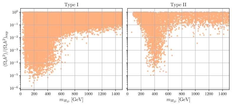
Figure 1: CN2HDM relic density normalised to the experimental value for type I (left) and type II (right) plotted against the DM mass $m_{H_{D}}$.

We start our phenomenological analysis of the model by investigating its interplay with DM observables. The most important DM observable is the DM relic density measured by the space telescope Planck [89]. We require valid parameter points to have a relic density that is under-abundant i.e. the predicted DM relic density is below or equal to the observed relic density by Planck,

$$(\Omega_{c}h^{2})_{\text{exp}}=0.1200\pm 0.0012\,.$$ (20)

Figure 1 depicts the obtained DM relic density values in the CN2HDM type I (left) and type II (right) normalised to the experimentally measured value versus the DM mass. The plot shows that in either Yukawa type the CN2HDM can account for the full relic abundance for all allowed $m_{H_{D}}$. In type I the lightest allowed $m_{H_{D}}$ are as low as $m_{H_{D}}=30~{}\text{GeV}$ with the highest allowed masses limited only by our scan range. In type II $m_{H_{D}}$ values below $62.5~{}\text{GeV}$ are exceedingly rare due to overall heavier mass spectra enforced by the interplay of flavour constraints and electroweak precision measurements. However, for any values of $m_{H_{D}}$ above that the type II CN2HDM can saturate the observed relic density as well. The overall heavier mass spectrum in type II is also the reason for the generally larger relic densities at low $m_{H_{D}}$ in type II compared to type I. Due to the large mass difference between the DM particle and the visible sector scalars that mediate its interactions the 2-to-2 scattering processes that deplete the relic density are less efficient.

Direct searches for DM particles have been and are being performed by various experimental collaborations. The current strongest bound on the spin-independent (SI) DM-nucleon scattering cross section — which is the relevant quantity for scalar mediators — was obtained by the XENON1T [90] experiment. Since the direct detection limits are derived assuming a DM relic density equivalent to the central experimental value of Eq. 20, they have to be rescaled to the relic density values predicted in our model as

$$\hat{\sigma}_{\text{DM-N}}=\sigma_{\text{DM-N}}\frac{\Omega_{c}h^{2}}{(\Omega_{c}h^{2})_{\text{exp}}}\,.$$ (21)

The resulting effective spin-independent (SI) DM-nucleon cross-section $\hat{\sigma}_{\text{DM-N}}$ is plotted against the DM mass in Fig. 2 (left) for type I and (right) for type II. The colour code denotes the fraction of the observed relic density predicted by our model.

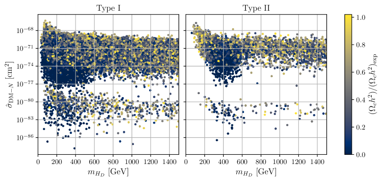
Figure 2: Effective SI direct detection DM-nucleon cross section $\hat{\sigma}_{\text{DM-N}}$ in cm² as a function of the DM mass $m_{H_{D}}$ for the CN2HDM type I (left) and type II (right).

Fig. 2 demonstrates that for both CN2HDM types the effective SI DM-nucleon cross section is heavily suppressed. All of the points are well below the neutrino-floor and hence are not in reach of direct detections experiments. The cross sections are suppressed by more than 20 orders of magnitude across the whole DM mass range compared to the upper limits on $\sigma_{SI}$ by XENON1T [90]. This is the consequence of a cancellation mechanism present in the CN2HDM, which makes the tree-level SI DM-nucleon cross section vanish in the limit of vanishing momentum transfer. The non-zero SI cross section values shown in Fig. 2 are due to higher-order QCD corrections taken into account by MicrOmegas which remain tiny due to the loop suppression. A simpler model realising this mechanism is discussed in Ref. [91], with electroweak corrections relevant for the SI cross section in this model discussed in Refs. [92, 93, 94]. This means that the CN2HDM can easily account for 100% of the observed DM density while remaining entirely out of reach of direct DM detection experiments.

Another way to investigate the dark sector is through invisible decays of particles at the collider. Current experimental measurements of the $h_{125}$ Higgs decaying to invisible particles place an exclusion limit on the Higgs $\to$ invisible branching ratio of 0.11 at 95% C.L. [95]. In Fig. 3 we show the invisible branching ratios obtained in the type I CN2HDM for all parameter points passing our constraints as a function of the SM-normalised signal rate $\mu_{VV}$ in the massive gauge boson final states $V\equiv Z,$ $W^{\pm}$. The colour code indicates the different $h_{125}$ scenarios, namely for the blue points $h_{125}$ is the lightest of the neutral non-DM Higgs bosons, $H_{1}$, for the yellow points it is $h_{125}\equiv H_{2}$, the green ones refer to $h_{125}\equiv H_{3}$ and the red points denote scenarios where the heaviest Higgs boson, $H_{4}$, is $h_{125}$. The $\mu_{VV}$ rate cannot be smaller than 0.855 in any scenario. The figure shows that for all allowed $\mu_{VV}$ values the branching ratio remains below the direct experimental upper limit of 0.11 so that the Higgs rate measurements in SM final states are still the most limiting constraints on the invisible decay width of $h_{125}$. In the CN2HDM, however, the direct limit from searches for $h_{125}\to\text{invisible}$ is not far from being competitive. For future conclusive statements it will therefore become necessary to include higher-order corrections in the computation of the related branching ratio. We found a similar behaviour as the one shown in Fig. 3 for the dark phases of the N2HDM [64], where the Higgs-to-invisible branching ratio remains below 10% after applying all Higgs constraints.

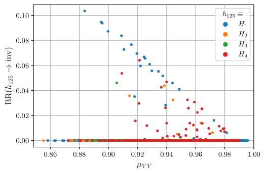
Figure 3: Type I: The branching ratio of the $h_{125}$ decaying into a pair of DM particles, for all types of $h_{125}$ mass ordering, plotted against the signal rate $\mu_{VV}$ into a massive gauge boson pair ($V\equiv Z,W^{\pm}$).

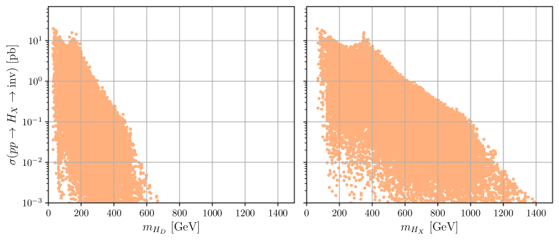
Figure 4: Type I: The production rate of all visible neutral Higgs bosons $H_{X}$ ($X=1,2,3,4$) with subsequent decay into invisible particles as function of the DM mass $m_{H_{D}}$ (left), and as function of the mass of the decaying Higgs boson $m_{H_{X}}$ (right).

In the CN2HDM type II, only $H_{1}$ can be the SM-like Higgs $h_{125}$. All other scenarios where $h_{125}$ is not the lightest neutral scalar in the visible sector are already excluded by the present constraints. We find $\text{BR}(h_{125}\to\text{invisible}<10\%)$ in the type II version of the model as well. However, for the vast majority of the valid parameter points in type II $m_{H_{D}}>62.5~{}\text{GeV}$ such that the branching ratio is zero.

In Fig. 4 we show for the CN2HDM type I the production cross sections of all visible neutral Higgs bosons, $H_{X}$ ($X=1,2,3,4$), i.e. also the non-SM-like ones, times their subsequent decay into invisible particles,

$$\sigma(pp\to H_{X}\to\mbox{inv})=\sigma(\text{ggF + bbH})\times\mbox{BR}(H_{X}\to\mbox{inv})\,,$$ (22)

plotted against $m_{H_{D}}$ (left) and against the mass $m_{H_{X}}$ of the decaying particle (right). All production cross sections have been computed at $\sqrt{s}=13$ TeV with SusHi v1.6.1 [96, 97] and are the sum of gluon production and associated production with a bottom quark pair. For most of the points — particularly those with the largest rates — the invisible decay is the dominant decay mode of $H_{X}$, often with branching ratios above 90%. In such a scenario a search in invisible final states may well be the only possibility to discover that particle. As can be inferred from the plot, the maximum cross section values at the lower end of the mass spectrum amount up to 25 pb which is reached for the case where $H_{4}=h_{125}$ in the decay $H_{2}\to$ invisible. We observe a dip at $m_{X}\approx 250$ GeV. Here the heavier non-SM-like Higgs bosons predominantly decay into a pair of SM-like $h_{125}$ Higgs bosons instead of a DM pair. This region corresponds to $m_{H_{D}}\approx 110$ GeV in the left plot. After increasing again to maximum values around $m_{H_{X}}=350$ GeV where the gluon fusion production cross section peaks, the rates quickly fall with increasing $H_{X}$ mass. Still, for heavy Higgs mass values of 1 TeV they amount up to 100 fb. They cross 1 fb at $m_{H_{X}}=1.4$ TeV.

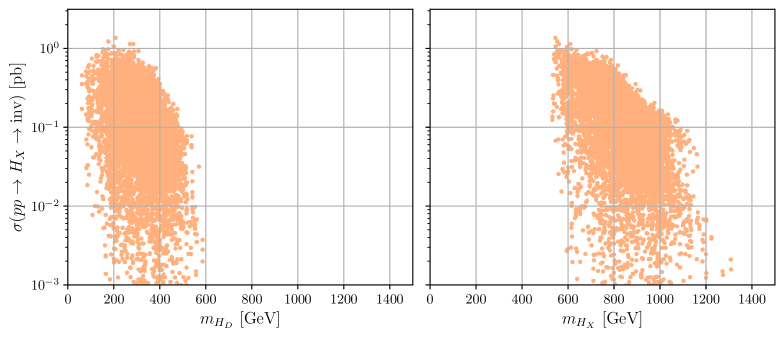
Figure 5: Type II: The production rate of all neutral Higgs bosons $H_{X}$ ($X=1,2,3,4$) with subsequent decay into invisible particles as function of the DM mass $m_{H_{D}}$ (left), and as function of the mass of the decaying Higgs boson $m_{H_{X}}$ (right).

Fig. 5 shows the same rates as Fig. 4 but for type II instead of type I Yukawa sectors. In type II, the neutral non-SM like Higgs masses $H_{2,3,4}$ are overall pushed to larger values, mainly due to the interplay of flavour and electroweak precision constraints. These also exclude scenarios with $m_{H_{D}}\leq 62.5$ GeV apart from very rare cases as stated above. With an overall heavier spectrum the rates are smaller than in the type I CN2HDM and reach at most 1.3 pb.

5 LHC Phenomenology of the CN2HDM Higgs Bosons

We now want to investigate the collider phenomenology in our model. The specific phenomenological feature of $h_{125}$ in our model is the possibility of non-vanishing singlet and/or CP-odd admixtures to the SM-like Higgs mass eigenstate which will affect its couplings and hence its production and decay rates. While we delay a detailed study of the phenomenology of the non-SM-like Higgs bosons to a future work, we will also comment on the overall mass spectra and their typical phenomenology. We first discuss the phenomenology of a type I CN2HDM in some detail and then comment on the differences in type II.

5.1 The Type I Higgs Mass Spectrum

If $h_{125}\equiv H_{1}$ the visible non-SM-like Higgs bosons can decouple with all masses becoming large and similar. In this scenario, the maximum allowed values of $m_{H_{2,3,4}},m_{H^{\pm}}$ are only limited by our scan ranges. Decoupling is no longer possible if $h_{125}$ is not the lightest of the neutral scalars and the Higgs mass spectrum becomes increasingly lighter as $h_{125}\equiv H_{2,3,4}$. Thus for $H_{2}\equiv h_{125}$ the maximum values of $m_{H_{3,4},H^{\pm}}$ are just above 600 GeV. Moreover, we now have an additional light Higgs in the spectrum with masses as low as $m_{H_{1}}=50$ GeV, where again the lower limits are determined by the lower limits of our scan ranges. For the case with $H_{3}\equiv h_{125}$, $m_{H_{4}}$ reaches at most 415 GeV and $m_{H^{\pm}}$ remains below 270 GeV. Additionally, we have two light visible Higgs masses in the spectrum with masses below 125 GeV and lower limits of $m_{H_{1}}=53$ GeV and $m_{H_{2}}=70$ GeV. For $H_{4}\equiv h_{125}$ the heaviest visible Higgs boson is the charged one with a maximum mass value of $m_{H^{\pm}}=190$ GeV. The three lighter Higgs bosons below 125 GeV have lower limits of 55 GeV, 68 GeV and 82 GeV for $m_{H_{1}}$, $m_{H_{2}}$ and $m_{H_{3}}$, respectively.

Let us give a brief generic overview of the signatures of the non-SM-like Higgs bosons. The main decay channels of the neutral Higgs bosons with masses below 125 GeV are those into lighter fermions and into a photon pair, depending on the respective mass values. The neutral visible Higgs bosons above 125 GeV mainly decay into top quark pairs, a neutral Higgs plus $Z$ boson pair, a charged Higgs plus $W^{\pm}$ pair, or into a pair of lighter neutral Higgs bosons. The specific decay channel depends on the involved coupling and mass values.

The charged Higgs boson decays, depending on the charged Higgs couplings and mass values, mainly into a top plus bottom quark pair, into a $\tau$ lepton and its associated neutrino, or into a neutral Higgs plus $W^{\pm}$ pair.

$\alpha_{1}$	$\alpha_{2}$	$\alpha_{3}$	$\alpha_{4}$	$\alpha_{5}$	$\alpha_{6}$	$\tan\beta$
1.386	-0.048	1.263	-0.028	1.395	0.0041	5.996
$m_{H_{a}}$ [GeV]	$m_{H_{b}}$ [GeV]	$m_{H_{D}}$ [GeV]	$m_{H^{\pm}}$ [GeV]	$v_{s}$ [GeV]	$\mbox{Re}(m_{12}^{2})$ [GeV2]
125.09	346.13	1472	578.97	477.92	43713

$m_{H_{3}}$ [GeV]	$m_{H_{4}}$ [GeV]	$\sigma_{\text{prod}}(H_{4})$ [fb]	BR($H_{4}\to H_{1}H_{2}$)	BR($H_{2}\to H_{1}H_{1}$)
516.83	532.02	97.23	0.463	0.577

Table 3: Type I: Input parameter values where $H_{a}\equiv H_{1}$ and $H_{b}\equiv H_{2}$ (top) and further information (bottom) on the $H_{1}H_{1}H_{1}$ benchmark point.

A smoking gun signature for extended Higgs sectors with more than two neutral visible Higgs bosons (i.e. more than in a 2HDM) would be Higgs-to-Higgs cascade decays. In the case with $H_{1}\equiv h_{125}$ we can e.g. find a triple SM-like Higgs $H_{1}H_{1}H_{1}$ production signature at a rate of $\sigma_{\text{prod}}(H_{4})\times\mbox{BR}(H_{4}\to H_{1}H_{2})\times\mbox{BR}(H_{2}\to H_{1}H_{1})=26$ fb. The input values for this benchmark point as well as additional information on the remaining neutral Higgs mass values, the $H_{4}$ production cross section and the involved Higgs-to-Higgs branching ratios are given in Tab. 3.

5.2 The Type I SM-Like Higgs Singlet and CP-odd Admixtures

We define the singlet and CP-odd components of $h_{125}$ through the respective elements in the mixing matrix $R$, namely,

singlet admixture: $$\quad R_{h_{125},3}^{2}\,,$$ (23)

CP-odd admixture: $$\quad R_{h_{125},4}^{2}\,.$$

This means that the singlet (CP-odd) admixture is given by the matrix element at the row associated with $h_{125}$ and the column associated with $s$ ($\rho_{3}$).

$h_{125}\equiv$	$H_{1}$	$H_{2}$	$H_{3}$	$H_{4}$
singlet admixture [%]	12.3	9.5	9.3	8.1
CP-odd admixture [%]	6.2	7.1	6.0	2.9

Table 4: Type I: The singlet and CP-odd admixture of the SM-like Higgs boson in % for the four different cases of $h_{125}\equiv H_{1,2,3,4}$.

In Table 4 we list the maximal separately reachable singlet and CP-odd admixtures of $h_{125}$ for the four different cases of $h_{125}\equiv H_{1,2,3,4}$ that are still in agreement with all constraints. The largest singlet component (12.3%) is reached for $h_{125}=H_{1}$ and decreases for lighter Higgs mass spectra. The maximum CP-odd admixture (7%) is obtained for $h_{125}\equiv H_{2}$. Figure 6 shows the impact of the CP-odd admixture on the fermionic ($\mu_{\tau\tau}=\mu_{bb}$ in type I) and bosonic signal strengths of $h_{125}$. We find that the CP-odd admixture decreases towards the lower and upper limits of $\mu_{VV}$ and $\mu_{\tau\tau}$. The maximum values are reached on the diagonal around $\mu_{\tau\tau}=\mu_{VV}\approx 0.92-0.94$. Figure 7 shows the corresponding plot for the singlet admixture. As the singlet component has no couplings to any SM particles, the singlet admixture decreases $\mu_{VV}$ and $\mu_{\tau\tau}$ simultaneously. This is clearer for $\mu_{VV}$ since $c^{2}(h_{125}VV)<1$ and therefore the coupling cannot be enlarged to counteract the singlet effects. For the fermion coupling this is possible leading to points with substantial singlet admixture also at larger $\mu_{\tau\tau}$.

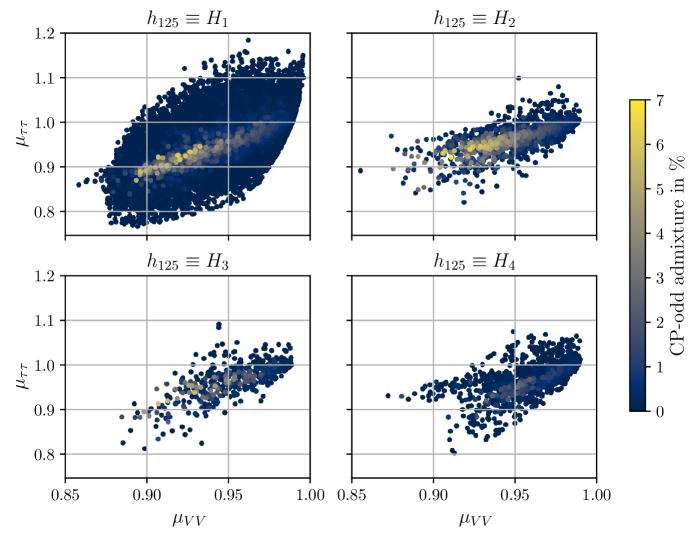
Figure 6: Type I: The rate $\mu_{\tau\tau}$ versus $\mu_{VV}$ for $H_{1,2,3,4}$ being SM-like, respectively, with the colour code denoting the CP-odd admixture.

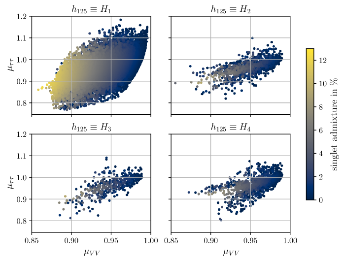
Figure 7: Type I: The rate $\mu_{\tau\tau}$ versus $\mu_{VV}$ for $H_{1,2,3,4}$ being SM-like, respectively, with the colour code denoting the singlet admixture.

5.3 The Type I SM-Like Higgs Rates

Since our model has an alignment limit, there are parameter sets where all $h_{125}$ couplings to fermions and gauge bosons are very close to the SM ones. We hence have to look for deviations in the Higgs rates from the SM-case that are specific in our model. In Tab. 5 we summarise the ranges that are still compatible with all constraints in the production rates $\mu_{\tau\tau}=\mu_{bb}$, $\mu_{VV}$, and $\mu_{\gamma\gamma}$ for the four different $h_{125}$ scenarios. As can be inferred from the table, the maximum freedom is given for the case where $H_{1}\equiv h_{125}$. In all $h_{125}$ scenarios the $\mu_{\tau\tau}$ range can exceed the SM-value (with the largest possible value of 1.18 obtained for $H_{1}$ being SM-like). The maximum Higgs rates into gauge bosons are $\leq 1$ for $h_{125}\equiv H_{1,...,4}$. As for the $\gamma\gamma$ rates, the lower limits in all four scenarios are about the same. However, the upper limit is largest for $H_{1}$ and equal to 1.14. In the other three cases the upper $\mu_{\gamma\gamma}$ is $\leq 1.04$. This is the result of the interplay between the trilinear Higgs self-coupling $\lambda_{h_{\text{125}}H^{+}H^{-}}$ and the mass of the charged Higgs boson running in the loop of the loop-induced Higgs coupling to the photons.

	$H_{1}$	$H_{2}$	$H_{3}$	$H_{4}$
$\mu_{\tau\tau}$	$0.77-1.18$	$0.82-1.11$	$0.81-1.09$	$0.80-1.08$
$\mu_{VV}$	$0.86-1.00$	$0.86-0.99$	$0.88-0.99$	$0.87-0.99$
$\mu_{\gamma\gamma}$	$0.83-1.14$	$0.82-1.04$	$0.82-1.01$	$0.82-1.02$

Table 5: Type I: The maximal and minimal signal rates of $h_{125}$ compatible with all applied constraints for the four different cases of $h_{125}\equiv H_{1,2,3,4}$.

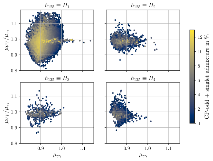
Figure 8: Type I: The rates ratio $\mu_{VV}/\mu_{\tau\tau}$ versus $\mu_{\gamma\gamma}$ for $H_{1,2,3,4}$ being SM-like, respectively, with the colour code denoting the combined CP-odd and singlet admixture.

Figure 8 shows the ratio $\mu_{VV}/\mu_{\tau\tau}$ plotted against $\mu_{\gamma\gamma}$, with the colour code denoting the combined CP-odd and singlet admixture of the $h_{125}$ given by $R_{h_{125},3}^{2}+R_{h_{125},4}^{2}$. The highest combined admixtures found in the four cases are $12.3\%$ when $h_{125}=H_{1}$, $10.9\%$ when $h_{125}=H_{2}$, $9.6\%$ when $h_{125}=H_{3}$ and $7.8\%$ when $h_{125}=H_{4}$. These values tend to be dominated by the singlet admixture, and the highest values of the singlet (CP-odd) admixture of the $h_{125}$ are accompanied by low values of the CP-odd (singlet) admixture, cf. Fig. 9.

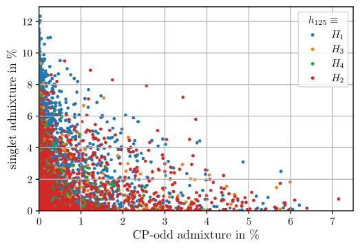
Figure 9: Type I: The singlet admixture versus the CP-odd admixture in % for $H_{1}\equiv h_{125}$ (blue), $H_{2}\equiv h_{125}$ (orange), $H_{3}\equiv h_{125}$ (green), and $H_{4}\equiv h_{125}$ (red).

We furthermore observe that the $\mu_{VV}$ and $\mu_{\tau\tau}$ values become increasingly correlated with rising CP-odd plus singlet admixtures so that their ratio is closer to 1 with larger admixtures. The large mixing case is hence barely distinguishable from the SM-case in this ratio. In the $\mu_{\gamma\gamma}$ rate a faint trend to smaller admixtures can be observed towards the edges of its allowed range. We furthermore clearly observe that $\mu_{\gamma\gamma}$ ranges above 1 require $\mu_{VV}/\mu_{\tau\tau}$ values close to 1 for $H_{1}\equiv h_{125}$ whereas this is less pronounced in the other scenarios, which, however, also have smaller maximal $\mu_{\gamma\gamma}$ values.

In summary, deviations in the individual $\mu_{\tau\tau}$ and $\mu_{VV}$ rates correlate with non-zero CP-odd and/or singlet admixtures, whereas their ratio does not allow us to make conclusive statements about these admixtures. The latter can also be said about the $\mu_{\gamma\gamma}$ rate. The photonic rates, however, allow us to distinguish the $h_{125}$ scenarios. Values of above 1.04 point towards $H_{1}\equiv h_{125}$. Furthermore, $\mu_{\gamma\gamma}$ values above 1 with $\mu_{VV}/\mu_{\tau\tau}$ deviating by more than about 0.2% from the SM ratio 1 may be a sign of $H_{2,3,4}$ being SM-like.

5.4 The CN2HDM Type II

In the CN2HDM type II, only points where the lightest visible neutral Higgs boson is the $h_{125}$ survive the constraints. The highest combined CP-odd-singlet admixture coincides with the highest singlet admixture at $19.3\%$ and is higher than in type I. The CP-odd admixture can become as large as 9%. The reason for larger allowed admixtures is that in the type II model the couplings to up- and to down-type fermions are disentangled and we hence have more freedom in the production and decay rates to accommodate larger non-SM admixtures to $h_{125}$ without violating the Higgs constraints. The $\mu_{\tau\tau}$ range is somewhat smaller than in the type I case with $H_{1}\equiv h_{125}$, lying between 0.76 and 1.13. The $\mu_{\tau\tau}$ rate is found to increase with increasing CP-odd admixture as we have an additional CP-odd-like coupling contributing to the Higgs-Yukawa interaction of the SM-like Higgs, and to decrease with increasing singlet admixture. The allowed $\mu_{VV}$ rate lies between 0.87 and 1.10 and thus clearly exceeds the upper limit allowed in type I. An enhancement of $\mu_{VV}$ is possible in type II since the coupling of $h_{125}$ to down-type quarks — and thus the dominant $h_{125}\to b\bar{b}$ decay width and the total width — can be reduced without simultaneously reducing the $t\bar{t}$ coupling that dominates the gluon fusion production cross section. The allowed $\mu_{\gamma\gamma}$ range is nearly identical to the one of $\mu_{VV}$, and neither of the two rates shows any sensitivity to the non-SM-like admixtures.

In Fig. 10 we depict the signal strength fraction $\mu_{VV}/\mu_{\tau\tau}$ versus $\mu_{\gamma\gamma}$ for all type II points passing our constraints. The colour code indicates the combined CP-odd and singlet admixture. The ratio $\mu_{VV}/\mu_{\tau\tau}$ can reach values of up to $1.35$ which are significantly higher than in the CN2HDM type I. At the same time, the lower bound of $0.87$ is also slightly higher than in type I. The ratio $\mu_{VV}/\mu_{\tau\tau}$ shows a dependence on the combined CP-odd and singlet admixtures in contrast to type I, and increases with increasing non-SM-like admixtures.

In summary, while we cannot use $\mu_{\gamma\gamma}$ to distinguish type I and type II, we can use $\mu_{\tau\tau}$ and $\mu_{VV}$ and in particular their ratio. Furthermore, contrary to type I, the ratio measurement of $\mu_{VV}$ and $\mu_{\tau\tau}$ allows for conclusions on non-SM-like admixtures to the SM-like Higgs boson.

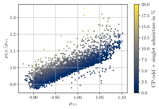
Figure 10: Type II: The rates ratio $\mu_{VV}/\mu_{\tau\tau}$ versus $\mu_{\gamma\gamma}$ for $H_{1}$ being SM-like, the only case compatible with the constraints. The colour code denotes the combined CP-odd and singlet admixture.

6 Conclusions

In this work we have introduced the CN2HDM. It is based on the CP-violating 2HDM extended by a complex singlet field that obeys a discrete $\mathbb{Z}_{2}$ symmetry. Thereby we obtain a model that implements all ingredients required to answer the most pressing open questions of the SM: It contains a DM candidate and it features CP violation, one of the three Sakharov conditions required for successful baryogenesis. After working out the relevant equations, we have implemented the model in ScannerS and used that implementation to perform scans in the parameter space of the model by simultaneously taking into account the relevant theoretical and experimental constraints. We investigated the type I and the type II version of the model and analysed the interplay between DM observables and the LHC phenomenology of the model. For the latter, we provided the code CN2HDM_HDECAY for the computation of the CN2HDM Higgs boson decay widths and branching ratios including state-of-the-art higher-order corrections.

The Higgs spectrum of the CN2HDM consists of a stable DM candidate, four visible CP-mixing neutral Higgs bosons and a pair of oppositely charged Higgs states. We found significant differences between the possible mass spectra of the CN2HDM type I and II. In type I the overall spectra can range from heavy decoupled BSM particles with only one SM-like scalar at $125~{}\text{GeV}$ to very light spectra with the heaviest of the four neutral scalars at $125~{}\text{GeV}$. In type II, however, the interplay of flavour and electroweak precision constraints always leads to rather heavy mass spectra where the lightest neutral scalar is always at $125~{}\text{GeV}$.

Investigating the DM properties of the model, we found that in either Yukawa type the model can easily account for 100% of the observed relic density. Due to a cancellation in the tree-level direct detection cross sections the model at the same time remains completely out of reach of direct DM searches. However, this does not make it impossible to probe the dark sector of the CN2HDM. We found that for a Yukawa sector of type I the branching ratio of the observed Higgs boson $h_{125}$ into a pair of DM particles can reach about 10.6% after taking into account the LHC Higgs measurements. This is just below the direct experimental upper limit for Higgs to invisible decays. With these limits getting stronger and stronger, it becomes clear that in the future higher-order electroweak corrections will have to be included in the prediction for the Higgs-to-invisible branching ratio to be able to draw meaningful conclusions on the still allowed Higgs coupling values. In type II the heavier mass spectra also influence the allowed DM masses, such that DM masses below $m_{h_{125}}/2$ are extremely rare. The decay rates of the non-SM-like Higgs bosons into DM particles can be quite large depending on their mass values. They reach 25 pb in type I and 1.3 pb in type II which has an overall heavier mass spectrum. For many parameter points one or more of the non-SM-like Higgs bosons decay almost exclusively into invisible final states, which could be the only feasible decay channel to discover those particles.

The non-minimal Higgs sector of the model allows for a rich LHC phenomenology. In type I all four visible neutral Higgs bosons can play the role of the discovered Higgs boson, meaning that e.g. if the heaviest one, $H_{4}$, is the SM-like Higgs boson, we have three visible light neutral Higgs bosons with masses below $125~{}\text{GeV}$ in the spectrum. We thus have a large variety of possible Higgs decays and signatures. In particular, spectacular Higgs-to-Higgs cascade decays with multiple Higgs bosons in the final state are possible with rates above $1{~{}\text{fb}}$. In the type II version on the other hand, the overall heavier Higgs spectra only allow for the lightest neutral non-DM Higgs boson to be the SM-like one. At the same time, since in the type II CN2HDM the up- and down-type fermions couple to two different Higgs doublets the SM-like Higgs boson can have larger CP-odd and singlet admixtures than the corresponding Higgs in type I while still being in agreement with all constraints. The CP-odd admixture can be up to 9% and the singlet admixture can reach 19% compared with the corresponding type I values of 7% and 12%, respectively. The combined CP-odd-singlet admixture reaches 12.5% in type I and 19% in type II. Both Yukawa types can predict deviations from the SM in the signal strengths of $h_{125}$ that could be observed at the HL-LHC or at a future collider. Distinguishing between the Yukawa types based on signal strength measurements alone is challenging, but may be possible, in particular if the signal rates are found to be larger than one.

With the CN2HDM we have presented an interesting benchmark model that can solve some of the most pressing open questions in the SM. The next steps will be further systematic investigations of its collider and DM phenomenology in order to identify signatures to discover the whole Higgs spectrum, and signatures that are specific for the model, i.e. smoking gun signatures, to distinguish it from other models. Observables that allow probing the amount of CP violation in the model also warrant investigation. Finally, while the model offers all of the required ingredients, it remains to be shown whether electroweak baryogenesis can indeed be realised through a sufficiently strong first order electroweak phase transition. The first step is done, the model is introduced and we have provided and published the required tools so that anyone interested can study the CN2HDM. Now further work is needed to corner the model experimentally and theoretically.

Appendix

Appendix A The $4\times 4$ Higgs Mixing Matrix

The orthogonal 4-dimensional mixing matrix is given by ($x,y=a,b,c,d$; $i,j=1,2,3,4$)

$$R_{xy}=R_{ij}=R=\begin{pmatrix}R_{11}&R_{12}&R_{13}&R_{14}\\ R_{21}&R_{22}&R_{23}&R_{24}\\ R_{31}&R_{32}&R_{33}&R_{34}\\ R_{41}&R_{42}&R_{32}&R_{44}\end{pmatrix},$$ (24)

where $R$ is parametrised by the order and direction of rotation of the angles $\alpha_{1},\alpha_{2},\alpha_{3},\alpha_{4},\alpha_{5},\alpha_{6}$ about the $\{x,y,z,w\}$ axes.

When we rotate in 4 dimensions, we rotate in each of the $x-y,x-z,x-w,y-z,y-w,z-w$ planes. We can modify our parametrisation of $R$ depending on which $\alpha_{i}$ characterises which plane of rotation and in which order we choose to rotate about our axes. There is no evident parametrisation in 4 dimensions, only that it is desirable to obtain a parametrisation giving rise to 4 conditions that easily allow us to describe the unique mixing matrix.

We choose the parametrisation

$$R=\begin{aligned} &R(\alpha_{4},\{x,z\})\cdot R(\alpha_{5},\{x,y\})\cdot R(-\alpha_{3},\{x,w\})\\ &\cdot R(\alpha_{6},\{y,z\})\cdot R(-\alpha_{2},\{y,w\})\cdot R(\alpha_{1},\{z,w\}),\end{aligned}$$ (25)

where $R(\alpha,\{p,q\})$ denotes a rotation in the plane $\{p,q\}$ characterised by $\alpha$. This choice yields the matrix comprised of the elements

$$R_{11} =c_{\alpha_{1}}c_{\alpha_{2}}c_{\alpha_{6}}$$ (26a)

$$R_{12} =c_{\alpha_{2}}c_{\alpha_{6}}s_{\alpha_{1}}$$ (26b)

$$R_{13} =c_{\alpha_{6}}s_{\alpha_{2}}$$ (26c)

$$R_{14} =-s_{\alpha_{6}}$$ (26d)

$$R_{21} =-s_{\alpha_{1}}(c_{\alpha_{3}}c_{\alpha_{4}}+s_{\alpha_{3}}s_{\alpha_{4}}s_{\alpha_{5}})+c_{\alpha_{1}}(-s_{\alpha_{2}}(c_{\alpha_{4}}s_{\alpha_{3}}-c_{\alpha_{3}}s_{\alpha_{4}}s_{\alpha_{5}})-c_{\alpha_{2}}c_{\alpha_{5}}s_{\alpha_{4}}s_{\alpha_{6}})$$ (26e)

$$R_{22} =c_{\alpha_{1}}(c_{\alpha_{3}}c_{\alpha_{4}}+s_{\alpha_{3}}s_{\alpha_{4}}s_{\alpha_{5}})+s_{\alpha_{1}}(-s_{\alpha_{2}}(c_{\alpha_{4}}s_{\alpha_{3}}-c_{\alpha_{3}}s_{\alpha_{4}}s_{\alpha_{5}})-c_{\alpha_{2}}c_{\alpha_{5}}s_{\alpha_{4}}s_{\alpha_{6}})$$ (26f)

$$R_{23} =c_{\alpha_{2}}(c_{\alpha_{4}}s_{\alpha_{3}}-c_{\alpha_{3}}s_{\alpha_{4}}s_{\alpha_{5}})-c_{\alpha_{5}}s_{\alpha_{2}}s_{\alpha_{4}}s_{\alpha_{6}}$$ (26g)

$$R_{24} =-c_{\alpha_{5}}c_{\alpha_{6}}s_{\alpha_{4}}$$ (26h)

$$R_{31} =c_{\alpha_{5}}s_{\alpha_{1}}s_{\alpha_{3}}+c_{\alpha_{1}}(-c_{\alpha_{3}}c_{\alpha_{5}}s_{\alpha_{2}}-c_{\alpha_{2}}s_{\alpha_{5}}s_{\alpha_{6}})$$ (26i)

$$R_{32} =-c_{\alpha_{1}}c_{\alpha_{5}}s_{\alpha_{3}}+s_{\alpha_{1}}(-c_{\alpha_{3}}c_{\alpha_{5}}s_{\alpha_{2}}-c_{\alpha_{2}}s_{\alpha_{5}}s_{\alpha_{6}})$$ (26j)

$$R_{33} =c_{\alpha_{2}}c_{\alpha_{3}}c_{\alpha_{5}}-s_{\alpha_{2}}s_{\alpha_{5}}s_{\alpha_{6}}$$ (26k)

$$R_{34} =-c_{\alpha_{6}}s_{\alpha_{5}}$$ (26l)

$$R_{41} =-s_{\alpha_{1}}(c_{\alpha_{3}}s_{\alpha_{4}}-c_{\alpha_{4}}s_{\alpha_{3}}s_{\alpha_{5}})+c_{\alpha_{1}}(-s_{\alpha_{2}}(s_{\alpha_{3}}s_{\alpha_{4}}+c_{\alpha_{3}}c_{\alpha_{4}}s_{\alpha_{5}})+c_{\alpha_{2}}c_{\alpha_{4}}c_{\alpha_{5}}s_{\alpha_{6}})$$ (26m)

$$R_{42} =c_{\alpha_{1}}(c_{\alpha_{3}}s_{\alpha_{4}}-c_{\alpha_{4}}s_{\alpha_{3}}s_{\alpha_{5}})+s_{\alpha_{1}}(-s_{\alpha_{2}}(s_{\alpha_{3}}s_{\alpha_{4}}+c_{\alpha_{3}}c_{\alpha_{4}}s_{\alpha_{5}})+c_{\alpha_{2}}c_{\alpha_{4}}c_{\alpha_{5}}s_{\alpha_{6}})$$ (26n)

$$R_{43} =c_{\alpha_{2}}(s_{\alpha_{3}}s_{\alpha_{4}}+c_{\alpha_{3}}c_{\alpha_{4}}s_{\alpha_{5}})+c_{\alpha_{4}}c_{\alpha_{5}}s_{\alpha_{2}}s_{\alpha_{6}}$$ (26o)

$$R_{44} =c_{\alpha_{4}}c_{\alpha_{5}}c_{\alpha_{6}}\,,$$ (26p)

where the $4\times 4$ matrix reduces to the standard $3\times 3$ rotation matrix as in Eq. (2.15) of Ref. [45] when $\alpha_{4,5,6}\rightarrow 0$. Without loss of generality, we choose to work in the convention where

$$-\pi/2\leq\alpha_{i}\leq\pi/2\,,$$ (27)

which always yields $\cos{\alpha_{i}}\geq 0$. The four conditions constraining the matrix are given by

$$R_{11} =c_{\alpha_{1}}c_{\alpha_{2}}c_{\alpha_{6}}>0$$ (28)

$$R_{44} =c_{\alpha_{4}}c_{\alpha_{5}}c_{\alpha_{6}}>0$$ (29)

$$R_{33}+\frac{R_{13}\cdot R_{14}\cdot R_{34}}{1-R_{14}^{2}} =c_{\alpha_{2}}c_{\alpha_{2}}c_{\alpha_{5}}>0$$ (30)

Det(R) $$=1\,.$$ (31)

These allow expressing the mixing angles in terms of the rotation matrix elements as

$$\alpha_{6} =\arcsin(-R_{14})\,$$ (32a)

$$\alpha_{2} =\arcsin\left(\frac{R_{13}}{c_{\alpha_{6}}}\right)$$ (32b)

$$\alpha_{5} =\arcsin\left(-\frac{R_{34}}{c_{\alpha_{6}}}\right)$$ (32c)

$$\alpha_{4} =\arcsin\left(-\frac{R_{24}}{c_{\alpha_{5}}c_{\alpha_{6}}}\right)$$ (32d)

$$\alpha_{1} =\arcsin\left(\frac{R_{12}}{c_{\alpha_{2}}c_{\alpha_{6}}}\right)$$ (32e)

$$\alpha_{3} =\arcsin\left(\frac{R_{31}s_{\alpha_{1}}-R_{32}c_{\alpha_{2}}}{c_{\alpha_{5}}}\right)\,,$$ (32f)

where each angle is written in terms of $\arcsin$, to avoid a potential sign ambiguity of the angle that can arise from $\arccos$ functions (since $\cos(-x)=\cos(x)$).

Appendix B Relations between Lagrangian and Physical Parameters

Calculating the dependent Higgs mass values and reordering the mass set, we can then find the relations between the Lagrangian and the physical parameters of the model. Defining

$$X=R^{T}\mathrm{diag}(m_{H_{1}}^{2},m_{H_{2}}^{2},m_{H_{3}}^{2},m_{H_{4}}^{2})R$$ (33)

for convenience, we find the quartic couplings,

$$\lambda_{1}= \frac{X_{11}\cos\beta-\operatorname{Re}m_{12}^{2}\sin\beta}{v^{2}\cos^{3}\beta}$$ (34)

$$\lambda_{2}= \frac{X_{22}\sin\beta-\operatorname{Re}m_{12}^{2}\cos\beta}{v^{2}\sin^{3}\beta}$$ (35)

$$\lambda_{3}= \frac{2m_{H^{\pm}}^{2}}{v^{2}}+\frac{X_{12}-\operatorname{Re}m_{12}^{2}}{v^{2}\sin\beta\cos\beta}$$ (36)

$$\lambda_{4}= \frac{X_{44}-2m_{H^{\pm}}^{2}}{v^{2}}+\frac{\operatorname{Re}m_{12}^{2}}{v^{2}\cos\beta\sin\beta}$$ (37)

$$\operatorname{Re}\lambda_{5}= \frac{\operatorname{Re}m_{12}^{2}}{v^{2}\sin\beta\cos\beta}-\frac{X_{44}}{v^{2}}$$ (38)

$$\operatorname{Im}\lambda_{5}= \frac{-2X_{24}}{v^{2}\cos\beta}$$ (39)

$$\lambda_{6}= \frac{4X_{33}}{v_{s}^{2}}$$ (40)

$$\lambda_{7}= \frac{2X_{13}}{vv_{s}\cos\beta}$$ (41)

$$\lambda_{8}= \frac{2X_{23}}{vv_{s}\sin\beta}\,.$$ (42)

References

- [1] ATLAS, G. Aad et al., Phys. Lett. B716, 1 (2012), 1207.7214.
- [2] CMS, S. Chatrchyan et al., Phys. Lett. B716, 30 (2012), 1207.7235.
- [3] Planck, P. A. R. Ade et al., Astron. Astrophys. 594, A13 (2016), 1502.01589.
- [4] Particle Data Group, C. Patrignani et al., Chin. Phys. C 40, 100001 (2016).
- [5] Planck, R. Adam et al., Astron. Astrophys. 594, A1 (2016), 1502.01582.
- [6] WMAP, C. L. Bennett et al., Astrophys. J. Suppl. 208, 20 (2013), 1212.5225.
- [7] V. A. Kuzmin, V. A. Rubakov, and M. E. Shaposhnikov, Phys. Lett. 155B, 36 (1985).
- [8] A. G. Cohen, D. B. Kaplan, and A. E. Nelson, Nucl. Phys. B349, 727 (1991).
- [9] A. G. Cohen, D. B. Kaplan, and A. E. Nelson, Ann. Rev. Nucl. Part. Sci. 43, 27 (1993), hep-ph/9302210.
- [10] M. Quiros, Helv. Phys. Acta 67, 451 (1994).
- [11] V. A. Rubakov and M. E. Shaposhnikov, Usp. Fiz. Nauk 166, 493 (1996), hep-ph/9603208, [Phys. Usp.39,461(1996)].
- [12] K. Funakubo, Prog. Theor. Phys. 96, 475 (1996), hep-ph/9608358.
- [13] M. Trodden, Rev. Mod. Phys. 71, 1463 (1999), hep-ph/9803479.
- [14] W. Bernreuther, Lect. Notes Phys. 591, 237 (2002), hep-ph/0205279, [,237(2002)].
- [15] D. E. Morrissey and M. J. Ramsey-Musolf, New J. Phys. 14, 125003 (2012), 1206.2942.
- [16] A. D. Sakharov, Pisma Zh. Eksp. Teor. Fiz. 5, 32 (1967), [Usp. Fiz. Nauk161,61(1991)].
- [17] V. Silveira and A. Zee, Phys. Lett. B 161, 136 (1985).
- [18] J. McDonald, Phys. Rev. D 50, 3637 (1994), hep-ph/0702143.
- [19] C. P. Burgess, M. Pospelov, and T. ter Veldhuis, Nucl. Phys. B 619, 709 (2001), hep-ph/0011335.
- [20] T. D. Lee, Phys. Rev. D8, 1226 (1973).
- [21] Particle Data Group, M. Tanabashi et al., Phys. Rev. D 98, 030001 (2018).
- [22] G. C. Branco et al., Phys. Rept. 516, 1 (2012), 1106.0034.
- [23] N. G. Deshpande and E. Ma, Phys. Rev. D 18, 2574 (1978).
- [24] E. Ma, Phys. Rev. D 73, 077301 (2006), hep-ph/0601225.
- [25] R. Barbieri, L. J. Hall, and V. S. Rychkov, Phys. Rev. D 74, 015007 (2006), hep-ph/0603188.
- [26] L. Lopez Honorez, E. Nezri, J. F. Oliver, and M. H. G. Tytgat, JCAP 02, 028 (2007), hep-ph/0612275.
- [27] E. Lundstrom, M. Gustafsson, and J. Edsjo, Phys. Rev. D 79, 035013 (2009), 0810.3924.
- [28] E. M. Dolle and S. Su, Phys. Rev. D 80, 055012 (2009), 0906.1609.
- [29] L. Lopez Honorez and C. E. Yaguna, JCAP 01, 002 (2011), 1011.1411.
- [30] L. Lopez Honorez and C. E. Yaguna, JHEP 09, 046 (2010), 1003.3125.
- [31] A. Goudelis, B. Herrmann, and O. Stål, JHEP 09, 106 (2013), 1303.3010.
- [32] C. Bonilla, D. Sokolowska, N. Darvishi, J. L. Diaz-Cruz, and M. Krawczyk, J. Phys. G 43, 065001 (2016), 1412.8730.
- [33] F. S. Queiroz and C. E. Yaguna, JCAP 02, 038 (2016), 1511.05967.
- [34] I. F. Ginzburg, M. Krawczyk, and P. Osland, Two Higgs doublet models with CP violation, in International Workshop on Linear Colliders (LCWS 2002), 2002, hep-ph/0211371.
- [35] W. Khater and P. Osland, Nucl. Phys. B 661, 209 (2003), hep-ph/0302004.
- [36] A. W. El Kaffas, P. Osland, and O. M. Ogreid, Nonlin. Phenom. Complex Syst. 10, 347 (2007), hep-ph/0702097.
- [37] B. Grzadkowski and P. Osland, Phys. Rev. D 82, 125026 (2010), 0910.4068.
- [38] A. Arhrib, E. Christova, H. Eberl, and E. Ginina, JHEP 04, 089 (2011), 1011.6560.
- [39] A. Barroso, P. M. Ferreira, R. Santos, and J. P. Silva, Phys. Rev. D 86, 015022 (2012), 1205.4247.
- [40] S. Inoue, M. J. Ramsey-Musolf, and Y. Zhang, Phys. Rev. D89, 115023 (2014), 1403.4257.
- [41] K. Cheung, J. S. Lee, E. Senaha, and P.-Y. Tseng, JHEP 06, 149 (2014), 1403.4775.
- [42] D. Fontes, J. C. Romao, and J. P. Silva, JHEP 12, 043 (2014), 1408.2534.
- [43] D. Fontes, J. C. Romão, R. Santos, and J. P. Silva, JHEP 06, 060 (2015), 1502.01720.
- [44] C.-Y. Chen, S. Dawson, and Y. Zhang, JHEP 06, 056 (2015), 1503.01114.
- [45] D. Fontes et al., JHEP 02, 073 (2018), 1711.09419.
- [46] R. Boto, T. V. Fernandes, H. E. Haber, J. C. Romão, and J. a. P. Silva, Phys. Rev. D 101, 055023 (2020), 2001.01430.
- [47] D. Fontes and J. C. Romão, JHEP 06, 016 (2021), 2103.06281.
- [48] C.-Y. Chen, M. Freid, and M. Sher, Phys. Rev. D89, 075009 (2014), 1312.3949.
- [49] A. Drozd, B. Grzadkowski, J. F. Gunion, and Y. Jiang, JHEP 11, 105 (2014), 1408.2106.
- [50] M. Muhlleitner, M. O. P. Sampaio, R. Santos, and J. Wittbrodt, JHEP 03, 094 (2017), 1612.01309.
- [51] I. Engeln, P. Ferreira, M. M. Mühlleitner, R. Santos, and J. Wittbrodt, JHEP 08, 085 (2020), 2004.05382.
- [52] P. M. Ferreira, R. Santos, M. Mühlleitner, G. Weiglein, and J. Wittbrodt, JHEP 09, 006 (2019), 1905.10234.
- [53] D. Azevedo, P. Gabriel, M. Muhlleitner, K. Sakurai, and R. Santos, (2021), 2104.03184.
- [54] P. Basler, M. Mühlleitner, and J. Müller, JHEP 05, 016 (2020), 1912.10477.
- [55] P. Basler and M. Mühlleitner, Comput. Phys. Commun. 237, 62 (2019), 1803.02846.
- [56] P. Basler, M. Mühlleitner, and J. Müller, Comput. Phys. Commun. 269, 108124 (2021), 2007.01725.
- [57] R. Coimbra, M. O. P. Sampaio, and R. Santos, Eur. Phys. J. C73, 2428 (2013), 1301.2599.
- [58] P. M. Ferreira, R. Guedes, M. O. P. Sampaio, and R. Santos, JHEP 12, 067 (2014), 1409.6723.
- [59] M. Mühlleitner, M. O. P. Sampaio, R. Santos, and J. Wittbrodt, (2020), 2007.02985.
- [60] ATLAS, CMS, G. Aad et al., Phys. Rev. Lett. 114, 191803 (2015), 1503.07589.
- [61] Anyhdecay: library wrapping non-supersymmetric hdecay variants, https://jonaswittbrodt.gitlab.io/anyhdecay/.
- [62] A. Djouadi, J. Kalinowski, and M. Spira, Comput. Phys. Commun. 108, 56 (1998), hep-ph/9704448.
- [63] A. Djouadi, J. Kalinowski, M. Muehlleitner, and M. Spira, Comput. Phys. Commun. 238, 214 (2019), 1801.09506.
- [64] I. Engeln, M. Mühlleitner, and J. Wittbrodt, Comput. Phys. Commun. 234, 256 (2019), 1805.00966.
- [65] M. Krause, D. Lopez-Val, M. Muhlleitner, and R. Santos, JHEP 12, 077 (2017), 1708.01578.
- [66] M. Krause and M. Mühlleitner, Comput. Phys. Commun. 247, 106924 (2020), 1904.02103.
- [67] J. Horejsi and M. Kladiva, Eur. Phys. J. C 46, 81 (2006), hep-ph/0510154.
- [68] K. G. Klimenko, Theor. Math. Phys. 62, 58 (1985).
- [69] P. Bechtle, S. Heinemeyer, O. Stål, T. Stefaniak, and G. Weiglein, Eur. Phys. J. C74, 2711 (2014), 1305.1933.
- [70] P. Bechtle et al., Eur. Phys. J. C 81, 145 (2021), 2012.09197.
- [71] P. Bechtle, O. Brein, S. Heinemeyer, G. Weiglein, and K. E. Williams, Comput. Phys. Commun. 181, 138 (2010), 0811.4169.
- [72] P. Bechtle, O. Brein, S. Heinemeyer, G. Weiglein, and K. E. Williams, Comput. Phys. Commun. 182, 2605 (2011), 1102.1898.
- [73] P. Bechtle et al., Eur. Phys. J. C 74, 2693 (2014), 1311.0055.
- [74] P. Bechtle, S. Heinemeyer, O. Stal, T. Stefaniak, and G. Weiglein, Eur. Phys. J. C 75, 421 (2015), 1507.06706.
- [75] P. Bechtle et al., Eur. Phys. J. C 80, 1211 (2020), 2006.06007.
- [76] J. Haller et al., Eur. Phys. J. C 78, 675 (2018), 1803.01853.
- [77] M. Misiak and M. Steinhauser, Eur. Phys. J. C77, 201 (2017), 1702.04571.
- [78] W. Grimus, L. Lavoura, O. M. Ogreid, and P. Osland, J. Phys. G35, 075001 (2008), 0711.4022.
- [79] W. Grimus, L. Lavoura, O. M. Ogreid, and P. Osland, Nucl. Phys. B801, 81 (2008), 0802.4353.
- [80] ACME, V. Andreev et al., Nature 562, 355 (2018).
- [81] G. Belanger, F. Boudjema, A. Pukhov, and A. Semenov, Comput. Phys. Commun. 176, 367 (2007), hep-ph/0607059.
- [82] G. Belanger, F. Boudjema, A. Pukhov, and A. Semenov, Comput. Phys. Commun. 180, 747 (2009), 0803.2360.
- [83] G. Belanger et al., Comput. Phys. Commun. 182, 842 (2011), 1004.1092.
- [84] G. Belanger, F. Boudjema, A. Pukhov, and A. Semenov, Comput. Phys. Commun. 185, 960 (2014), 1305.0237.
- [85] G. Bélanger, F. Boudjema, A. Pukhov, and A. Semenov, Comput. Phys. Commun. 192, 322 (2015), 1407.6129.
- [86] D. Barducci et al., Comput. Phys. Commun. 222, 327 (2018), 1606.03834.
- [87] G. Bélanger, F. Boudjema, A. Goudelis, A. Pukhov, and B. Zaldivar, Comput. Phys. Commun. 231, 173 (2018), 1801.03509.
- [88] G. Belanger, A. Mjallal, and A. Pukhov, Eur. Phys. J. C 81, 239 (2021), 2003.08621.
- [89] Planck, N. Aghanim et al., Astron. Astrophys. 641, A6 (2020), 1807.06209.
- [90] XENON, E. Aprile et al., Phys. Rev. Lett. 121, 111302 (2018), 1805.12562.
- [91] C. Gross, O. Lebedev, and T. Toma, Phys. Rev. Lett. 119, 191801 (2017), 1708.02253.
- [92] D. Azevedo et al., JHEP 01, 138 (2019), 1810.06105.
- [93] K. Ishiwata and T. Toma, JHEP 12, 089 (2018), 1810.08139.
- [94] S. Glaus et al., JHEP 12, 034 (2020), 2008.12985.
- [95] ATLAS, M. Aaboud et al., (2020), ATLAS-CONF-2020-052.
- [96] R. V. Harlander, S. Liebler, and H. Mantler, Comput. Phys. Commun. 184, 1605 (2013), 1212.3249.
- [97] R. V. Harlander, S. Liebler, and H. Mantler, Comput. Phys. Commun. 212, 239 (2017), 1605.03190.