figurec

Sub-femtosecond optical control of entangled states

Abstact

Entanglement is one of the most fascinating aspects distinguishing quantum from classical physics [1]. It is the backbone of quantum information processing [2] which relies on engineered quantum systems. It also exists in natural systems such as atoms and molecules, showcased in many experimental instances [3] mostly in the form of entangled photon pairs [4, 5, 6] and a few examples of entanglement between massive particles [7, 8, 9, 10, 11]. Nevertheless, the control of entanglement in natural systems has never been demonstrated. In artificially prepared quantum systems, on the other hand, the creation and manipulation of entanglement lies at the heart of quantum computing [12] currently implemented in a wide array of two-level systems (e.g. trapped ions [13, 14, 15], superconducting [16] and semiconductor systems [17]). These processes are, however, relatively slow: the time scale of the entanglement generation and control ranges from a couple of $\mu s$ in case of trapped-ion quantum systems [18] down to tens of ns in superconducting systems [16]. In this letter, we show ultrafast optical control of entanglement between massive fundamental particles in a natural system on a time scale faster than that available to engineered systems. We demonstrate the sub-femtosecond control of spatially-separated electronic entangled states in a single hydrogen molecule by applying few-photon interactions with adjustable relative delays and a coincidence detection scheme. This molecular entanglement is revealed in the asymmetric electron emission with respect to the bound electron in the photodissociation of H₂. We anticipate that these results open the way to entanglement-based operations at THz speed.

Main

Molecular dissociation provides a unique platform to study entanglement since this latter may be encoded in the many different degrees of freedom of a molecule. An essential step in realizing the applications of molecules in quantum science is to demonstrate entanglement involving an individual molecule [19]. In addition to quantum information science, investigation of entanglement between massive particles as a result of a molecular breakup is of interest to quantum theory since it resembles the original idea of Einstein, Podolsky, and Rosen [20]. Over a decade ago, pioneering experimental examples showed the effect of molecular entanglement where entangled particle pairs were produced in molecular dissociation [10, 11] using synchrotron radiation. However, the tailored control of these processes has remained an experimental challenge due to the molecular dynamics which are governed by electrons moving on an attosecond time scale [21]. So far, the effect of entanglement and control of it has been indirectly studied in loss of coherence in the composite quantum system of photoelectron/ion as a result of photoionization in atoms or molecules by detection of only one particle [22, 23, 24, 25, 26, 27, 28]. We show that such challenges can be overcome with a combination of photoionization with ultra-short light pulses and a single-event two-particle coincidence measurement scheme. In the following, we introduce an ultrafast optical generation of entangled electronic state which can be controlled on a sub-femtosecond time scale.

We focus on the following entangled states

$$\ket{\psi}=\alpha_{o}\ket{+,-}+\beta_{o}e^{i2\phi(\tau)}\ket{-,+},$$ (1)

$$\ket{\phi}=\alpha_{e}\ket{+,+}+\beta_{e}e^{i2\phi(\tau)}\ket{-,-},$$ (2)

analogous to the four Bell states $\ket{\psi_{B}^{\pm}}=\frac{1}{\sqrt{2}}(\ket{+,-}\pm\ket{-,+})$ and $\ket{\phi_{B}^{\pm}}=\frac{1}{\sqrt{2}}(\ket{+,+}\pm\ket{-,-})$, where $\ket{j_{1},j_{2}},j_{i}\in\{+,-\}$ denotes the combined state of the bipartite system. For our demonstration, we consider $j$ as the parity of an electronic state, but the conceptual idea is more general. $\alpha_{o/e}$ and $\beta_{o/e}$ are complex numbers. As we demonstrate below, we control the phase $\phi$ (see Fig. 1) with the delay ($\tau$) between photons on a sub-fs ($10^{-15}s$) time scale. The distribution of photons and their relative timing among the excitation pathways (shown as arrows in Fig. 1) determines which of Bell states are generated.

We demonstrate this ultrafast generation and control of entanglement in the two-electron system of the hydrogen molecule. The starting point is the H₂ ground state. The final state is a superposition of electronic states with either positive $\ket{+}$ or negative $\ket{-}$ parity for each electron. We use the notation $\ket{\textit{parity of the bound, parity of the free electron}}$ throughout this work. Once in one of the Bell states, the value of the phase $\phi$ manifests itself in an asymmetric emission direction of the free electron with respect to the hydrogen atom containing the other, still bound electron, during the photodissociation of H₂ with $n$ photons

$$H_{2}+n\gamma\;\rightarrow\;H^{+}\;+\;H\;+\;e^{-}.$$ (3)

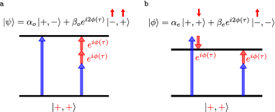
Figure 1: Generation scheme for Bell states using few-photon interactions. Schematic illustration of the generation of entangled Bell states using a combination of high- (blue arrows) and low-frequency photons (red arrows) from a well-defined state $\ket{+,+}$ in the ground state of molecular hydrogen. Distribution of photons among excitation pathways determines the generation of a specific Bell state.

The emission direction of the photoelectron is symmetric and shows no preferred direction with respect to the ejected neutral hydrogen atom if the inversion symmetry (parity) of the electron wave function is well-defined during dissociation. However, the molecular system can be placed in a superposition of states with opposite parities which leads to an asymmetric electron emission [29]. So far, this effect, which is the result of a phase difference in the coherent superposition of two dissociative pathways, has been observed by single-photon dissociative photoionization [11, 30] where the control of the asymmetry (phase) from outside is not possible. We show that one can steer the asymmetric emission of the photoelectron by using a few-photon interaction with different colors in combination with control of their relative delay on a sub-femtosecond time scale. This effect should not be confused with the localization of the bound electron on one of the nuclei in the laboratory frame using a spatially asymmetric strong laser field during dissociation as reported in [31, 32, 33]. In those experiments only proton/deuteron is detected and their ejection direction with respect to the laser polarization is controlled by the phase of the light field irrespective of the direction of the ejected photoelectron. For instance, in the seminal work of Sansone et al. the ejection direction of the proton is controlled (laboratory-frame asymmetry) using the delay between XUV and strong IR pulses and is demonstrated by detecting only the proton/deuteron. In our experiment, however, we demonstrate the signature of entanglement in the bipartite system of photoelectron/ion by detecting them in coincidence while they are spatially separated and steer their entangled ejection direction using the delay between XUV and week IR pulses.

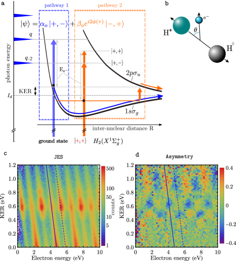
Figure 2: Interaction of XUV and IR photons with a hydrogen molecule: the energy sharing spectogram and asymmetry histograms. a, Schematic illustration of dissociation channels of H₂ with a combination of XUV (blue arrows) and IR (red arrows) photons. The ground state of H₂ ($X^{1}\Sigma^{+}_{g}$) is a well defined state denoted $\ket{+,+}$. The ground state ($1s\sigma_{g}$) and the first excited state ($2p\sigma_{u}$) of the molecular ion (H${}_{2}^{+}$) are shown with black curves. The dissociation limit ($I_{d}$) is shown with the horizontal gray dashed line. Two indistinguishable dissociation pathways 1 and 2 add up coherently to the same final state, namely the same electron energy (E${}_{e^{-}}$) and KER. b Schematic illustration of the dissociative photoionization of H₂. $\theta$ is the emission angle of the photoelectron with respect to the H⁺ emission direction. c, Joint energy spectrum (JES) for the dissociative ionization of H₂ with a combination of XUV and IR light. An even band (EB) is shown with a diagonal solid line as a result of the absorption of XUV photons with an energy of 25.2 eV. The absorption of XUV+IR photon results in an even band (EB) marked with a diagonal dashed line. The enhancement of the signal at a KER of 0.6 eV is due to the absorption of an IR photon by the molecular ion (bond softening). d The asymmetry parameter A in the case of dissociation with XUV and IR photons. A is non-zero in the region between KER 0.35 to 1.2 eV. The two diagonal lines, indicating an OB and EB, serve as a guide.

We determine the emission asymmetry from the angular distribution of the photoelectron with respect to the ejected neutral hydrogen atom containing the bound electron after dissociation of H${}_{2}^{+}$ by detecting the electron and proton in coincidence using a REMI apparatus [34] where the neutral hydrogen atom is ejected opposite to the direction of the proton. The spectrometer consists of two position-sensitive detectors for electrons and ions. We can retrieve the 3D momentum components of ions and electrons using time-of-flights and hit positions on the detectors. Our light source is a femtosecond laser with a central wavelength of 1030 nm (IR) and a pulse duration of 50 fs. The whole beam is split into two arms. The main part is used to produce photons in the ultraviolet (XUV) spectral region with energies up to 40 eV using high-harmonic generation [35]. A schematic spectrum of a selected region of the XUV radiation is shown in Fig. 2a. The spectrum consists of equally-distanced spikes where the energy difference between them is 2 IR photons (2 $\times$ 1.2 eV). The remaining weaker part is delayed in time and overlapped spatially and temporally with the XUV pulse. Both pulses interact with a gas jet of H₂ in the REMI. Our experimental principle is similar to [36]. The main process is single-ionization of H₂ into the molecular ion ground state (1$s\sigma_{g}$). Only a small fraction of ionization events lead to dissociation for photons with energies higher than the dissociation limit of H₂ (I_d=18.1 eV). We detect for each dissociation event a proton ($H^{+}$) and an electron in coincidence and obtain the energy and momentum (K) of them. The energy of the not detected neutral $H$ is reconstructed using momentum conservation K${}_{H}+$K${}_{H^{+}}+$K${}_{e^{-}}=0$. After dissociation, unlike atoms, the energy of the incoming photon can be distributed among electronic and nuclear degrees of freedom:

$$\overbrace{E_{H^{+}}+E_{H}}^{\text{KER}}+E_{e^{-}}=E_{\gamma}-I_{d},$$ (4)

where $I_{d}$ is the dissociation limit. The sum of the energy of the proton and hydrogen atom ($E_{H^{+}}+E_{H}$) is referred to as kinetic energy release (KER). In order to visualize the distribution of the absorbed photon energy between nuclei and electron, we plot KER vs electron energy ($E_{e^{-}})$ in a 2D histogram (joint energy spectrum (JES)). The JES for photodissociation of H₂ with a combination of XUV and IR photons is shown in Fig. 2c for a KER region from 0 to 1.2 eV. Due to energy conservation most events appear on diagonal lines with a slope of -1. Two types of such lines exist: odd bands (OBs), mainly caused by single-XUV-photon absorption and even bands (EBs) caused by XUV-IR two-photon absorption. For example, absorption of XUV photons with an energy of 25.2 eV results in a total energy of $25.2-18.1=7.1$ eV shared between electron and nuclei resulting in events on an OB highlighted by a diagonal solid line. A combination of XUV and IR photons results in an EB marked with a diagonal dashed line. The enhancement of the dissociation signal at a KER of around 0.6 eV is due to a process known as bond softening [37].

In order to quantify the asymmetric electron emission, corresponding to the phase $\phi$ in Eq.1, we define the asymmetry parameter A

$$A=\frac{N_{\theta<90}-N_{\theta>90}}{N_{\theta<90}+N_{\theta>90}},$$ (5)

with $\theta$ being the electron emission angle with respect to the ejected proton as shown in Fig. 2b. $N_{\theta<90}$ and $N_{\theta>90}$ are the number of events where the electron and proton are emitted in the same and the opposite hemisphere, respectively. A plot of parameter A for events in Fig. 2c is shown in Fig. 2d. For a KER of 0.35 eV we observe that the electron has a preferential direction with respect to the emitted proton (A is non-zero) for all electron energies. Additionally, OBs and EBs show different trends.

The asymmetric electron emission occurs in the region where the contribution of the ground-state dissociation (pathway 1) and the bond softening (pathway 2) overlap (KER from 0.35 to 1.2 eV). A more complete treatment is provided in the supplementary material section 3.

In case of OBs (see supplementary material section 2.1.1 for EBs), in pathway 1 (Fig. 2a), an XUV photon ($\gamma_{q}$ where $q$ is the harmonic order) with an energy higher than $I_{d}$ can lead to dissociation through 1s$\sigma_{g}$ with KERs<2 eV. The electron energy will be $E_{e^{-}}=\gamma_{q}-I_{d}-KER$ and the parity of the bound and continuum electron becomes gerade $\ket{+}$ and ungerade $\ket{-}$, respectively. In pathway 2 , the molecule is first ionized, to the ground state of the molecular ion ($1s\sigma_{g}$) with a next lower harmonic photon ($\gamma_{q-2}$) of the XUV spectrum compared to pathway 1. This process happens in the presence of a weak IR probe field where the photoelectron absorbs a photon instantaneously leading to an energy $E_{e^{-}}=\gamma_{q-2}+\hbar\omega-E_{b}$ where $E_{b}$ is the energy of the bound vibrational level in the ground state of the molecular ion. The symmetry of the emitted photoelectron after absorption of one IR photon becomes gerade ($\ket{+}$). The molecular ion, containing the bound electron, absorbs also an IR photon and the molecule dissociates along the repulsive $2p\sigma_{u}$ ionic state leaving the bound electron with ungerade symmetry ($\ket{-}$). The condition for quantum interference is fulfilled, namely that the energy of both electron and KER are the same for both pathways. Hence, we write the final wave function in the form of Eq. 1 as a coherent superposition of the two pathways 1 and 2 where $\alpha_{o}$ and $\beta_{o}$ are the probability amplitudes of pathway 1 and 2, respectively. The vibrational nuclear wave-function can be omitted in the final wave function since it is always of gerade symmetry in case of H₂, and is also the same for both pathways for the same KER.

Knowing the contributing pathways, Eq. 5 can be rewritten in terms of the coefficient $\alpha_{o}$ and $\beta_{o}$ by using appropriate bases according to [30]

$$A=\frac{-2|\alpha_{o}||\beta_{o}|\text{cos}\big{(}\text{arg}[\alpha_{o}]-\text{arg}[\beta_{o}]-2\phi(\tau)\big{)}}{|\alpha_{o}|^{2}+|\beta_{o}|^{2}},$$ (6)

where $\phi$ is the phase difference between XUV and IR fields. This shows that the asymmetry A is not only a function of $\alpha_{o}$ and $\beta_{o}$, but also the delay which can be controlled in our experiment. We also retrieve the coefficients $\alpha_{o/e}$ and $\beta_{o/e}$ (see supplementary material section 3.3.2).

In order to show the time dependence, we add all the OBs together (see supplementary material section 3.3) and subtract the time-averaged asymmetry. The resulting asymmetry is plotted as a function of the delay between XUV and IR photons in Fig. 3a. The oscillation of the asymmetry parameter A as a function of the delay with a period of 1.7 fs at a given KER demonstrates the sub-femtosecond laser control of the phase $\phi$ of the entangled states of Eq. 1. The experimental results are very well reproduced (Fig. 3b) with a numerical simulation based on the WKB (Wentzel–Kramers–Brillouin) approximation (see supplementary material section 3.3).

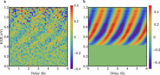
Figure 3: Time-dependent asymmetry parameter: experiment vs. simulation. The asymmetry parameter as a function of the delay between XUV and IR pulses. Comparison between the experiment (a) and simulation based on the WKB approximation (b). For the simulation we plot Eq. 6 with retrieved $\alpha_{o}$ and $\beta_{o}$.

In conclusion, this proof-of-principle demonstration of femtosecond entanglement generation and sub-femtosecond control may open new directions for quantum manipulation and processing on ultrafast time scales. It will be interesting to apply this scheme to larger molecules or even solids, and thereby test quantum-dynamical theories describing effective decoherence effects arising e.g. due to coupling to complex electronic or internuclar/phononic degrees of freedom. It should be noted that for suitably chosen quantum systems even visible frequencies are sufficient to implement the same ultrafast control scheme.

Methods

Experimental methods

The output of a linearly-polarized fiber laser with a central wavelength of 1030 nm, a pulse energy of 1 mJ, and a pulse duration of 50 fs at a repetition rate of 50 kHz is divided into two beams with a 85/15 beam splitter and fed into an interferometer with a Mach-Zehnder configuration. The main 85 percent (pump arm) is focused into an argon gas jet for high-harmonic generation (HHG) with a plano-convex lens with a focal length of 500 mm. A 200-$\mu$m aluminum foil is used to filter the incoming infrared beam as well as the lower harmonics which results in the XUV spectrum shown schematically in Fig. S2 c in supplementary material. In the main text only a small region of the spectrum is shown for illustration purposes (see main text Fig. 2a. The remaining 15 percent (probe arm) is delayed in time by changing the length of the probe arm of the interferometer using a controllable piezoelectric linear translation stage. An iris is used to reduced the IR probe intensity to roughly $2\times 10^{11}$ $W/cm^{2}$ in order to avoid higher order photon-induced transitions during the experiment. Both arms are recombined and focused using a grazing-incidence 2f-2f toroidal mirror into a supersonic gas jet of randomly-oriented cooled $H_{2}$ molecules inside a reaction microscope (cold target recoil ion momentum spectroscopy (COLTRIMS))[38] where the background pressure is kept below $2\times 10^{-10}$ mbar. Both ions and electrons are guided towards position-sensitive detectors with the help of an electric field. A homogeneous magnetic field is also used to reach a $4\pi$-electron-detection efficiency. Momentum distributions of ions and electrons are obtained using the time of flight and the hit position on the detectors resulting in 3D momentum distributions which reveal the full kinematic information about the dissociation channels for each event. For an overview of the setup see Fig. S1 in the supplementary material.

Acknowledgments The authors acknowledge and thank A. Buchleitner and E. Brunner for useful discussions. We further thank D. Bakucz Canário for helpful discussions and comments on the manuscript.

Funding Max-Planck Society.

Author contributions F.S. designed and constructed the pump-probe XUV-IR beamline and performed measurements and data analysis. P.F. and A.H. developed the theoretical description and numerical calculations. H.S. and A.H. contributed to the design and setting up of the beamline. R.M. and T.P. conceived the idea and conceptual interpretation. All authors discussed the results and contributed to the preparation of the manuscript.

Competing interests The authors declare no competing interests.

Data availability Source data are provided with this paper. All other data that support the findings of this paper are available from the corresponding authors upon request.

supplementary material for
Sub-femtosecond optical control of entangled states

Farshad Shobeiry, Patrick Fross, Hemkumar Srinivas,
Thomas Pfeifer, Robert Moshammer, Anne Harth

1 Experimental setup

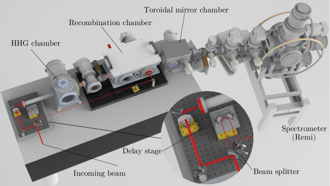
Figure 4: The attosecond XUV-IR setup. The incoming laser beam is divided into two beams using a 85/15 beam splitter. The main arm (85 percent of the beam) is focused into a gas jet for high-harmonic generation ion the HHG chamber. The remaining 15 percent (probe arm) is delay delayed in time by changing the optical length of the probe arm using a controllable linear translation state. Two arms are recombined in the recombination chamber and focused into the spectrometer.

The measurement was done at the attosecond beam (Fig. S 4) line at the Max Planck institute for nuclear physics. For the description of the interferometer see the methods section of the main text.

1.1 Momentum resolution

Due to its geometry the spectrometer has a slightly different momentum resolution for different momentum components. The maximum resolution is along the spectrometer axis (z component). Fig. S 5 and Fig. S 6 show the sum of ion-electron (H${}_{2}^{+}$-electron coincidence) momenta for the single-ionization channel in H₂. The width of the distributions is the measure of the momentum resolution.

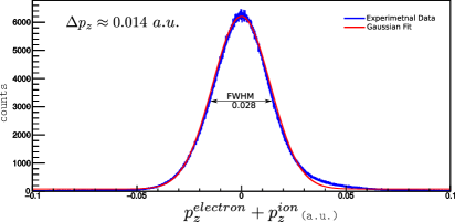
Figure 5: Sum of the longitudinal momentum components of electrons (e^-) and ions (H${}_{2}^{+}$) in the single ionization of H₂. Figure taken from [39].

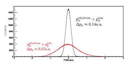
Figure 6: Momentum sum for the two transversal components of electrons (e^-) and ions (H${}_{2}^{+}$) in the single ionization of H₂. Figure taken from [39].

A dissociation event is determined by detecting an electron (e^-) and a proton (H⁺) in coincidence. We recorded the data with a rate of 15 protons per second and detected in total over 2.1 millions $H^{+}$ events in coincidence with electrons.

1.1.1 Reconstruction of the molecular frame

The detected recoil direction is the same as the dissociation direction at the moment of the interaction of the photon with the molecule based on axial recoil approximation [40]. All detected fragments are initially in the laboratory frame (LF) of reference. In photodissociation of H₂, the molecular frame momentum of proton is given by

$$\hat{\textbf{p}}^{H^{+}}_{MF}=\hat{\textbf{p}}^{H^{+}}_{LF}+\frac{1}{2}\hat{\textbf{p}}^{e^{-}}_{LF},$$ (7)

where $\hat{\textbf{p}}^{H^{+}}_{LF}$ and $\hat{\textbf{p}}^{e^{-}}_{LF}$ are the retrieved momentum vectors in the laboratory frame for the proton and electron, respectively. The neutral fragment of the dissociation (H) is not detected during our measurement. Using momentum conservation, however, we can reconstruct the momentum vectors of H in post-analysis. The momentum of the incoming photon is neglected since it is much smaller than the momenta of dissociation fragments and the spectrometer momentum resolution. For instance, the momentum of a 30-eV photon is only 0.008 a.u. (1 a.u. of momentum is equivalent to 1.995$\times 10^{-24}$ kg.m.s^-1) which is smaller than the momentum resolution of our spectrometer.

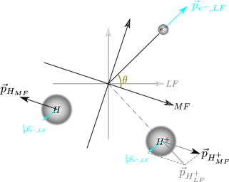
Figure 7: Schematic representation of the reconstruction of the molecular frame. Figure taken from [39].

2 Supplementary Text

2.1 Dissociation of H₂

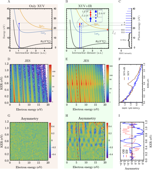
Figure 8: The relevant potential energy curves of H₂ are given in A) and B). The dissociation limit is marked with a horizontal dashed line at 18.1 eV. A) The schematic interaction of harmonic 21st with the hydrogen molecule. B) Dissociation of H₂ with the XUV photons in the presence of a weak IR field. The molecule is ionized and the photoelectron absorbs or emits an IR photon (red arrows). An IR photon can also couple the $1s\sigma_{g}$ to $2p\sigma_{u}$ at higher internuclear distances resulting in an enhancement in dissociation rate as a result of bond softening (BS). C) The schematic spectrum of the XUV light resulting from high-harmonic generation. Lower part of the spectrum is filtered out. D) JES for the dissociation of H₂ with XUV light. OB 21 is marked with a diagonal line with a slope of -1. E) JES for the dissociation of H₂ with XUV+IR pulses. An EB and OB is marked with dashed and solid lines, respectively. F) The projection of OB 21 onto the KER axis for dissociation with only XUV (blue curve) and XUV+IR photons (brown curve). G) Asymmetry parameter for dissociation event with only XUV pulse. H) The asymmetry parameter in the case of dissociation with XUV and IR Pulses. I) The asymmetry parameter for EB 20 and OB 21 are shown with dashed and solid curves, respectively.

Upon absorption of XUV photons with energies higher than the dissociation limit of H₂ (I_d=18.1 eV) the molecule can be ionized leading consecutively to the dissociation of the molecule. Fig. S 8A shows the schematic interaction of an XUV photon with H₂. This photon belongs to the 21th harmonic of the XUV spectrum with an energy of 25.2 eV. As a result, the molecule dissociates at the limit of the ionic state 1s$\sigma_{g}$ (ground-state dissociation (GD)). GD is the dominant dissociative channel for photon energies up to 27 eV [41]. GD leaves the ionic fragment with an energy less than 1 eV (KER<2 eV). The corresponding events from dissociation with harmonic 21th appear on a diagonal line marked with a solid line in the joint-energy spectrum (JES) histogram in Fig S 8D. Other lines in the JES correspond to other harmonics in the XUV spectrum. These lines are called odd bands (OBs) since an odd number of photons (in this case only one photon) is absorbed. The projection of the marked band onto the KER axis is shown with the blue curve in Fig S 8F.

The schematic interaction of a combination of an XUV and IR photons with H₂ is shown in Fig S 8B. In this case, one IR photon is absorbed or emitted (shown in the inset of panel B) by the photoelectron which results in events on diagonal lines (bands) between OBs. One example is marked with a dashed line in Fig. S 8E which we called an even band (EB) as a result of absorption of harmonic 19 plus an IR photon and absorption of harmonic 21 minus an IR photon.

In general, an additional photon can also be absorbed by the molecular ion due to bond softening at an internuclear distance (R) of around 5 a.u. where the 1s$\sigma_{g}$ and 2p$\sigma_{u}$ curves are energetically one IR photon apart.

The projection of the selected OB (marked with the brown solid line) in the case of the interaction with the XUV and IR photons is shown with the brown curve in panel F. We normalized the two curves at the KER around zero to emphasize the difference at a KER of around 0.6 eV. Note that, in this case, the region at KER $\approx$ 0.6 eV can be reached directly by one XUV photon (from harmonic 21) or by one XUV photon from the next lower harmonic (harmonic 19) plus two IR photons (one absorbed by the photoelectron and the other by the molecular ion) or by one XUV photon from the same 21st harmonic followed by the emission of an IR photon by the photoelectron and absorption of another IR photon by the molecular ion (see Fig. S10). The latter is a third path, omitted in the main text for simplicity, which leads to the same final symmetry ($\ket{-,+}$ in OBs ) as in the pathway 2.

The experimental results for the asymmetry parameter are shown in Fig. S 8G and H. Panel G shows that the asymmetry parameter is zero in the case of the dissociative ionization only with XUV photons. This is a sure sign that the asymmetric photoelectron emission takes place only when an interference of different dissociation pathways leading to the same final state is present. Whereas, in Fig. S 8H we observe asymmetric photoelectron emission in the overlap region. An important feature in Fig. S8 H, is the fact that all OBs show the same trend. The same is true for EBs. Another feature is that, the OBs and EBs are $\pi$ out of phase due to the extra absorbed photon by EBs. This feature is underlined in the projection of an odd and even band onto the KER axis in Fig. S 8I.

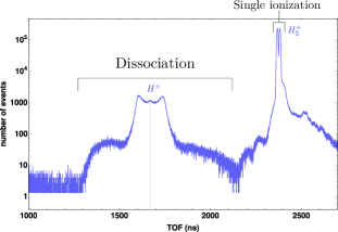
Figure 9: Time of flight spectrum of detected ions as a result of the interaction between a combination of XUV and IR pulses with H₂ molecules.

A time-of-flight (TOF) spectrum of the detected ions as a result of ionization of H₂ with XUV and IR photons is shown in Fig S9. This plot shows that the dominant interaction product is the single-ionization of the molecule.

2.1.1 Pathways in even bands

In case of EBs (see Fig. 1B of the main text), an XUV photon with an energy higher than I_d leads to dissociation through 1s$\sigma_{g}$ with KERs<2 eV. The photoelectron emits an IR photon leaving the electron energy $E_{e}=\gamma_{q}-I_{d}-KER-\hbar\omega$ and the parity of the bound and continuum electron becomes gerade $\ket{+}$. For the pathway including bond softening, the molecule is ionized with the next lower harmonic into the ground state of the molecular ion 1s$\sigma_{g}$. The photoelectron energy is in this case $E_{e}=\gamma_{q-2}-E_{b}$ with $E_{b}$ being the energy of the bound vibrational level in the ground state of the molecular ion. The parity of the photoelectron is ungerade $\ket{-}$. The molecular ion which contains the bound electron, absorbs an IR photon which promotes the molecular ion to the repulsive 2p$\sigma_{g}$ curve. The molecule eventually dissociates leaving the bound electron with ungerade parity $\ket{-}$.

2.2 Electron emission asymmetry

In this section we establish a connection between the asymmetry parameter (main text Eq. 5) and the coherent superposition of the dissociative pathways.

Since we have more than one pathway leading to the final state and these pathways are of two different natures, namely, ground-state dissociation and bond softening, we write the final state in a general manner in the form of

$$\ket{\psi}=c_{gs}\ket{+,-}+c_{bs}\ket{-,+},$$ (8)

for OBs and

$$\ket{\phi}=c_{gs}\ket{+,+}+c_{bs}\ket{-,-},$$ (9)

for EBs, where $c_{gs}$ and $c_{bs}$ are complex numbers. Both the amplitude and phase are relevant.

A superposition of molecular orbitals with different parities leads to the fact that the bound electron is localized either on the left or right sided of the nucleus. A similar spatial asymmetry happens also for the photoelectron using the superposition of spherical harmonics with either positive ($\ket{+_{e}}$) or negative ($\ket{-_{e}}$) parities (see [42]).

$$\includegraphics[keepaspectratio={true},scale={0.3}]{gradestate.png}\;+\;\includegraphics[keepaspectratio={true},scale={0.3},trim=0.0pt 91.04872pt 0.0pt 0.0pt]{ungradestate.png}\;=\;\includegraphics[keepaspectratio={true},scale={0.3},trim=0.0pt 42.67912pt 0.0pt 0.0pt]{product.png}$$ (10)

$$\includegraphics[keepaspectratio={true},scale={0.3}]{gradestate.png}\;-\;\includegraphics[keepaspectratio={true},scale={0.3},trim=0.0pt 91.04872pt 0.0pt 0.0pt]{ungradestate.png}\;=\;\includegraphics[keepaspectratio={true},scale={0.3},trim=0.0pt 42.67912pt 0.0pt 0.0pt]{product2.png}$$ (11)

As a result, we define a set of left-right bases as follows

$$\begin{split}\ket{H_{right}^{+}}&=\ket{+_{p}}+\ket{-_{p}},\\ \ket{H_{left}^{+}}&=\ket{+_{p}}-\ket{-_{p}},\\ \ket{e_{right}^{-}}&=\ket{+_{e}}+\ket{-_{e}},\\ \ket{e_{left}^{-}}&=\ket{+_{e}}-\ket{-_{e}}.\end{split}$$ (12)

This leads to the following four cases for the electron and proton combinations where we have two cases for both electron and proton emitted in the same direction and vice versa.

$$\begin{split}&\ket{\psi_{\theta<90}^{1}}=\ket{H_{right}^{+}}\otimes\ket{e_{right}^{-}},\qquad\qquad\includegraphics[keepaspectratio={true},scale={0.1},trim=0.0pt 184.9429pt 0.0pt 0.0pt]{pro1.png}\\ \\ &\ket{\psi_{\theta<90}^{2}}=\ket{H_{left}^{+}}\otimes\ket{e_{left}^{-}},\;\;\;\qquad\qquad\includegraphics[keepaspectratio={true},scale={0.1},trim=0.0pt 184.9429pt 0.0pt 0.0pt]{pro2.png}\\ \\ &\ket{\psi_{\theta>90}^{1}}=\ket{H_{right}^{+}}\otimes\ket{e_{left}^{-}},\;\qquad\qquad\includegraphics[keepaspectratio={true},scale={0.1},trim=0.0pt 184.9429pt 0.0pt 0.0pt]{anti1.png}\\ \\ &\ket{\psi_{\theta>90}^{2}}=\ket{H_{left}^{+}}\otimes\ket{e_{right}^{-}},\;\qquad\qquad\includegraphics[keepaspectratio={true},scale={0.1},trim=0.0pt 184.9429pt 0.0pt 0.0pt]{anti2.png}\end{split}$$ (13)

where $\theta$ is the angle between the photoelectron and the ejected proton (see Fig. 2C in the main text). The transition coefficients can be calculated by projecting the final state (Eq. S.2) onto different cases using above equations

$$\begin{split}\absolutevalue{\innerproduct{\psi_{\theta<90}^{1}}{\psi}}^{2}&=(c_{gs}+c_{bs})(c_{gs}^{*}+c_{bs}^{*}),\\ \absolutevalue{\innerproduct{\psi_{\theta<90}^{2}}{\psi}}^{2}&=(-c_{gs}-c_{bs})(-c_{gs}^{*}-c_{bs}^{*}),\\ \absolutevalue{\innerproduct{\psi_{\theta>90}^{1}}{\psi}}^{2}&=(-c_{gs}+c_{bs})(-c_{gs}^{*}+c_{bs}^{*}),\\ \absolutevalue{\innerproduct{\psi_{\theta>90}^{2}}{\psi}}^{2}&=(c_{gs}-c_{bs})(c_{gs}^{*}-c_{bs}^{*}).\end{split}$$ (14)

By definition, we write the number of dissociation events as:

$$\begin{split}N_{\theta<90}&=\absolutevalue{\innerproduct{\psi_{\theta<90}^{1}}{\psi_{f}}}^{2}+\absolutevalue{\innerproduct{\psi_{\theta<90}^{2}}{\psi_{f}}}^{2},\\ N_{\theta>90}&=\absolutevalue{\innerproduct{\psi_{\theta>90}^{1}}{\psi_{f}}}^{2}+\absolutevalue{\innerproduct{\psi_{\theta>90}^{2}}{\psi_{f}}}^{2}.\end{split}$$ (15)

Using the definition of the asymmetry parameter (Eq. 5 of the main text), we can rewrite A as a function of $c_{gs}$ and $c_{bs}$

$$\begin{split}A&=-\frac{2\text{Re}[c_{gs}c_{bs}^{*}]}{\absolutevalue{c_{gs}}^{2}+\absolutevalue{c_{bs}}^{2}}\\ &=-\frac{2\absolutevalue{c_{gs}}\absolutevalue{c_{bs}}\text{cos}(\phi_{gs}-\phi_{bs})}{\absolutevalue{c_{gs}}^{2}+\absolutevalue{c_{bs}}^{2}},\end{split}$$ (16)

where $\phi_{gs,bs}=\text{arg}[c_{gs},c_{bs}]$.

3 Model

In this section we introduce a model that supports that the origin of the time-dependent asymmetry lies in the interference of photoelectrons coming from GS and BS dissociation quantum pathways where at least two neighboring harmonics in the XUV spectrum are involved.

Many quantum pathways are involved in the experiment. However, for the GS and BS dissociation pathways we consider only the lowest photon transitions due to vanishing intensities of both XUV and IR pulses. These are shown in Fig. S10. All these paths interfere and have a contribution to the final dissociation probability, and affect the asymmetry parameter A.

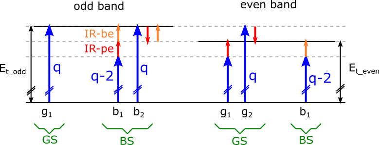
Figure 10: Quantum pathways for odd and even bands. The blue arrows represent the XUV photon with different discrete photon energies: e.g. $q-2$ is the next lower harmonic to $q$ with an energy difference of two IR photons. The red arrow represents an IR photon absorbed or emitted by the photoelectron (IR-pe), while the orange one represents an IR photon absorbed by the bound electron (IR-be) leading to bond softening.

For now, we consider odd bands and call the complex coefficients $g_{1}$ for the GS pathway, $b_{1}$ and $b_{2}$ for the BS pathway according to Fig. S10. Eq. 8 becomes

$$\ket{\psi}=g_{1}\ket{+,-}+(b_{1}+b_{2})\ket{-,+}.$$ (17)

Note that for pathway $g_{1}$ one photon and for pathways $b_{1}$ and $b_{2}$ three photons are involved. With this the dissociation probability reads:

$$P_{odd}=|g_{1}+b_{1}+b_{2}|^{2}.$$ (18)

The asymmetry parameter Eq. 16 becomes

$$\begin{split}A_{odd}&=\frac{-(g_{1}(b_{1}+b_{2})^{*}+(b_{1}+b_{2})g_{1}^{*})}{|b_{1}+b_{2}|^{2}+|g_{1}|^{2}}\\ &=\frac{-2(|g_{1}||b_{1}|\cos(\Delta\phi_{g_{1},b_{1}})+|g_{1}||b_{2}|\cos(\Delta\phi_{g_{1},b_{2}}))}{|g_{1}|^{2}+|b_{1}|^{2}+|b_{2}|^{2}+2|b_{1}||b_{2}|\cos(\Delta\phi_{b_{1},b_{2}})},\end{split}$$ (19)

with $\Delta\phi_{bi,bj}=\arg[b_{i}]-\arg[b_{j}]$ and $\Delta\phi_{gi,bj}=\arg[g_{i}]-\arg[b_{j}]$.

The complex coefficients correspond to the specific components of dipole transition element from the vibronic ground state to the continua [43]. Within the Franck-Condon (FC) approximation, the electronic and the nuclear components of the total wave function (Eq. 17) can be separated $\psi(r,R)=\chi(R)\phi(r,R)$. We neglect the dependence of the electronic matrix elements on the nuclear position. This leads to the complex expressions:

$$g_{1}=\underbrace{FC_{gs}\;\mathrm{e}^{\mathrm{i}\Theta_{gs}}}_{\begin{subarray}{c}nuclear\\ contribution\end{subarray}}\times\underbrace{M^{(1)}_{g1}}_{\begin{subarray}{c}photo-e\\ contribution\end{subarray}},$$ (20)

$$b_{1}=\underbrace{FC_{bs}\;\mathrm{e}^{\mathrm{i}\Theta_{bs}}}_{\begin{subarray}{c}nuclear\\ contribution\end{subarray}}\underbrace{{\color[rgb]{0,0,0}\mathrm{e}^{\mathrm{i}\phi(\tau)}}}_{\begin{subarray}{c}bound-e\\ contribution\end{subarray}}\times\underbrace{M^{(2)}_{b1}}_{\begin{subarray}{c}photo-e\\ contribution\end{subarray}},$$ (21)

$$b_{2}=\underbrace{FC_{bs}\;\mathrm{e}^{\mathrm{i}\Theta_{bs}}}_{\begin{subarray}{c}nuclear\\ contribution\end{subarray}}\underbrace{{\color[rgb]{0,0,0}\mathrm{e}^{\mathrm{i}\phi(\tau)}}}_{\begin{subarray}{c}bound-e\\ contribution\end{subarray}}\times\underbrace{M^{(2)}_{b2}}_{\begin{subarray}{c}photo-e\\ contribution\end{subarray}},$$ (22)

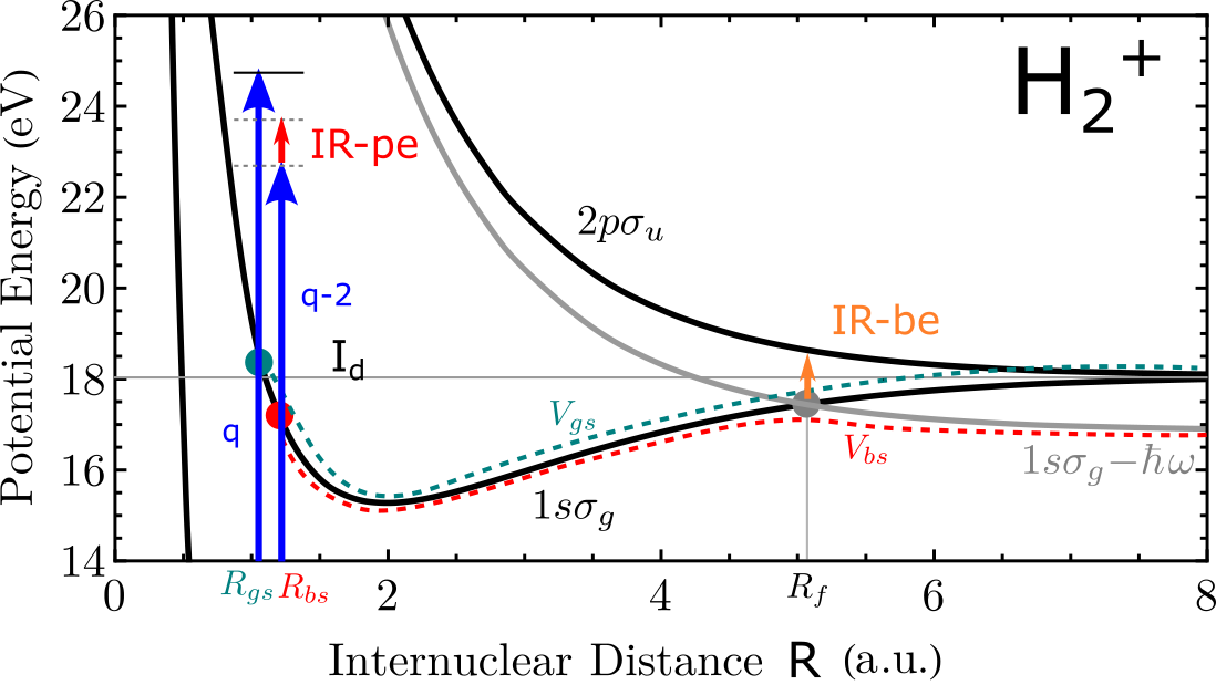
Figure 11: Schematic representation of the quantum paths $g_{1}$ and $b_{1}$ in the $H_{2}$ molecular potential curves. These two quantum paths are the most significant ones that lead to a time-dependent asymmetry in odd bands.

where $FC$ stands for a contribution that represents the nuclear part. The nuclear part has a phase $\Theta_{gs/bs}$. The contribution for the photoelectron is accounted for by the complex multi-photon matrix element $M^{(N)}$ where $N$ is the number of involved photon transitions. Bond softening is a photo-induced process. In order to account for the phase of this field, the phase of the IR field ($e^{i\phi(\tau)}$) is multiplied to the bond softening matrix element in Eq. S 15 and S 16.

3.1 WKB-phase

The phases $\Theta_{gs/bs}$ account for the accumulated phases of the nuclei moving in the given potential energy curves $V_{gs}$ and $V_{bs}$, see Fig. S11. The phases from the moving nuclei are estimated with the WKB (Wentzel–Kramers–Brillouin) approximation:

$$\Theta_{gs}=\int_{R_{gs}}^{\infty}dR\sqrt{2\mu(KER+I_{d}-V_{gs}(R))},$$ (23)

$$\Theta_{bs}=\int_{R_{bs}}^{\infty}dR\sqrt{2\mu(KER+I_{d}-V_{bs}(R))},$$ (24)

where the integrand is the nuclear momentum with $\mu$ being the reduced mass of H${}_{2}^{+}$.

Please note the different limits of the integrals. For ground-state dissociation, the phase $\Theta_{gs}$ is calculated by integrating from the internuclear distance $R_{gs}$ to the limit of $R\rightarrow\infty$ where the molecule dissociates long the 1s$\sigma_{g}$ curve with a KER of 0.6 eV. The phase of the pathway ($\Theta_{bs}$) is obtained by the integral in Eq. S18 which has a different lower limit since the process starts with the ionization of the molecule leaving the ion in the bound ground state. The integration pathway follows the laser-dressed potential curve (dashed red curve (V_bs)) at the limit of the adiabatic 1s$\sigma_{g}$-$\hbar\omega$ curve obtained by diagonalizing the diabatic potential matrix [44]. The width of the avoided crossings at R_f is obtained by taking into account the IR intensity during the measurement.

3.2 Phase of electric dipole matrix element

For this model approach, the electric dipole matrix elements, $M$, are approximated to be independent of $R$. According to the shown paths in Fig. S10, $M_{g1}^{(1)}$ describes a first-order perturbation process and $M_{b1}^{(2)},M_{b2}^{(2)}$ describe second-order perturbation processes. Although we deal with a real two-electron system, the single active electron approximation can be used [45], since the interaction with the light only changes the electronic state of the photo-electron; while the bound electron remains in the ground state of the molecular ion.

The complex electric dipole matrix elements (assuming only linearly polarized light) and their asymptotic phases can be written as ([46]):

$$M^{(1)}_{g1}(k;R_{gs}) =E_{\Omega_{q}}\sum_{\ell}\mathcal{M}^{(1)}_{\ell,0}(k)Y_{\ell,0}\quad\textrm{with} \mathrm{arg}[{M}_{g1}^{(1)}] =\phi_{q}^{XUV}-\frac{\pi}{2}-\frac{\pi\ell}{2},$$ (25)

$$M^{(2)}_{b1}(k;R_{bs}) =E_{\Omega_{q-2}}E_{\omega}\sum_{\ell}\mathcal{M}^{(2)}_{\ell,0}(k)Y_{\ell,0}\quad\textrm{with} \mathrm{arg}[{M}_{b1}^{(2)}] =\phi_{q-2}^{XUV}+\omega\tau-\frac{\pi\ell}{2},$$ (26)

$$M^{(2)}_{b2}(k;R_{bs}) =E_{\Omega_{q}}E_{-\omega}\sum_{\ell}\mathcal{M}^{(2)}_{\ell,0}(k)Y_{\ell,0}\quad\textrm{with} \mathrm{arg}[{M}_{b2}^{(2)}] =\phi_{q}^{XUV}-\omega\tau-\frac{\pi\ell}{2}.$$ (27)

Here, the atomic phase contribution including the Wigner and continuum-continuum couplings are neglected, since they are small compared to the atto-chirp [35]. The final photoelectron momentum $k$ and angular momentum $\ell$ are the same for all paths. $E_{\Omega/\omega}$ are the complex electric fields of the XUV and the IR pulses, $Y_{\ell,m}$ are the angular momentum and magnetic-quantum-number dependent spherical harmonics. $\mathcal{M}^{(N)}(k)$ is a complex expression that contains the radial part of the transition-matrix element. We can safely assume that the IR pulse $\arg[E_{\omega}]=\omega(t+\tau)+IR_{chirp}$ is not chirped and we set $t=0$: $\arg[E_{\omega}]=\omega\tau=\phi(\tau)$, With this, we write the phases of the complex amplitudes of the three quantum paths for odd bands:

$$\mathrm{arg}[g_{1}] =\Theta_{gs}-\frac{\pi}{2}-\frac{\pi\ell}{2}+\phi_{q}^{XUV} =\Phi_{g1},$$ (28)

$$\mathrm{arg}[b_{1}] =\Theta_{bs}-\frac{\pi\ell}{2}+\phi_{q-2}^{XUV}+2\phi(\tau) =\Phi_{b1}+2\phi(\tau),$$ (29)

$$\mathrm{arg}[b_{2}] =\Theta_{bs}-\frac{\pi\ell}{2}+\phi_{q}^{XUV} =\Phi_{b2}.$$ (30)

In order to get Eq. 1 in the main text we replace the complex coefficients in Eq. 17 with the defined phases above and their corresponding magnitudes to get $$\ket{\psi}=|g_{1}|\mbox{e}^{i\Phi_{g1}}\ket{+,-}+(|b_{1}|\mbox{e}^{i(\Phi_{b1}+2\phi(\tau))}+|b_{2}|\mbox{e}^{i\Phi_{b2}})\ket{-,+}.$$ (31) By setting $|g_{1}|\mbox{e}^{i\Phi_{g1}}=\alpha_{o}$, $|b_{1}|\mbox{e}^{i\Phi_{b1}}=\beta_{o}$, and neglecting pathway $b_{2}$ we get $$\ket{\psi}=\alpha_{o}\ket{+,-}+\beta_{o}\mbox{e}^{i2\phi(\tau)}\ket{-,+}.$$ (32) We discuss this simplification in order to focus on the time-dependence asymmetry. However, path $b_{2}$ is needed in order to explain all observed structures in the experiment. The asymmetry parameter (Eq. S.10) in this case becomes $$A=\frac{-2|\alpha_{o}||\beta_{o}|\text{cos}\big{(}\text{arg}[\alpha_{o}]-\text{arg}[\beta_{o}]-2\phi(\tau)\big{)}}{|\alpha_{o}|^{2}+|\beta_{o}|^{2}}.$$ (33) The same is repeated for even bands below.

In order to obtain an analytical expression for the asymmetry (Eq. 19), we need to know the phase differences between the three paths:

$$\begin{split}\Delta\phi_{g_{1},b_{1}}&=\Delta\Theta-\frac{\pi}{2}+\Delta\phi_{q,q-2}^{XUV}-2\phi(\tau),\\ \Delta\phi_{g_{1},b_{2}}&=\Delta\Theta-\frac{\pi}{2},\\ \Delta\phi_{b_{1},b_{2}}&=+\Delta\phi_{q-2,q}^{XUV}+2\phi(\tau),\end{split}$$ (34)

where $\Delta\phi_{i,j}^{XUV}=\phi_{i}^{XUV}-\phi_{j}^{XUV}$ is the chirp of the XUV pulse, and $\Delta\Theta=\Theta_{gs}-\Theta_{bs}$ is the phase difference resulting from the nuclear part (WKP phase) of the wave function.

The time dependent asymmetry reads:

$$A_{odd}(\tau)=\frac{-2|g_{1}||b_{1}|\sin(\Delta\Theta+\Delta\phi_{q,q-2}^{XUV}-2\phi(\tau))-2|g_{1}||b_{2}|\sin(\Delta\Theta)}{|g_{1}|^{2}+|b_{1}|^{2}+|b_{2}|^{2}+2|b_{1}||b_{2}|\cos(\Delta\phi_{q,q-2}^{XUV}-\phi(\tau))},$$ (35)

and the time-averaged asymmetry parameter is not zero: $<A>=\int d\tau A(\tau)\neq 0$.

It is worth discussing the role of the different considered quantum paths $g_{1},b_{1}$,and $b_{2}$. If $|g_{1}|$ is zero, the asymmetry parameter is zero and the time-dependent population probability shows a similar form of a RABBITT-like experiment [47, 35]. If $|b_{1}|$ is zero, the asymmetry parameter is not time dependent. This shows that, in order to see a time dependence in the experiment, two interfering quantum paths need to involve two neighboring XUV frequencies. If $|b_{2}|$ is zero, the asymmetry parameter is time dependent but the time average asymmetry parameter is zero. Only if all three paths are present we obtain what the experiment shows:

• a $\tau$-dependent asymmetry parameter $A(\tau)$

• and a non zero time average $\langle A\rangle=\int d\tau A(\tau)\neq 0$.

That is why we know that at least these three lowest-order perturbation paths need to be considered in order to model the experimental results. However, for the discussion in the main text about the origin of the time-dependent asymmetry two paths are sufficient.

3.3 Experiment

Fig. S 12 shows the experimental time-averaged asymmetry parameter ($\langle A\rangle$) as a function of KER for the first three odd bands (OBs). They correspond to harmonic 17th (OB1), 19th (OB2), and 21st (OB3). The black line is the theoretical curve ($\langle A\rangle$) based on the model explained above. For the simulation we used the retrieved amplitudes for $g_{1}$, $b_{1}$, and $b_{2}$ explained in the following section. For $\phi(\tau)=\omega\tau$ we know the photon energy (1.2 eV), and therefore, $\omega$. Before plotting the experimental asymmetry parameter as a function of the time delay, we add all OBs together in order to improve the statistics. The bands are slightly shifted in time with respect to each other mainly due to the chirp of the XUV pulse. This chirp is a function of the photon energy. We retrieve the XUV spectral phase from a reference measurement done on argon. The spectral phase (phase difference) is shown as a function of the photon energy in Fig S17. We repeat the same procedure for EBs. The resulted plots for the asymmetry parameter are shown in Fig. S 13A, and Fig. S 16A for odd and even bands, respectively.

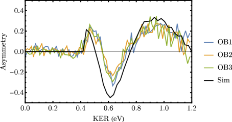
Figure 12: Experimental time-integrated odd-band asymmetry parameter ($\langle A\rangle$) as a function of KER. Black curve shows the asymmetry A based on Eq. 35 with $|g_{1}|=\alpha_{o}$ and $|b1+b2|=\beta_{o}$.

Fig. S 13 C) and D) shows the asymmetry minus the mean time-averaged contribution $A(\tau)-\langle A(\tau)\rangle$ for OBs for both the experiment and theory. Fig. S 16 C) and D) show that of the EBs.

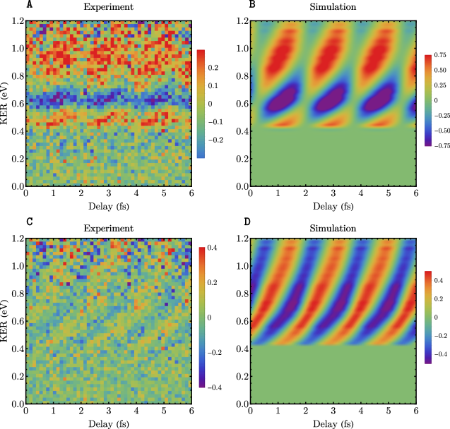
Figure 13: Odd band: A) and C) Experiment, B) and D) simulation based on the model. A) and B): The asymmetry parameter as a function of the delay between the XUV and IR pulses. Comparison between the experiment and the model based on the WKB approximation shows a good agreement. C) and D): Asymmetry minus the mean time-independent part ($A-\langle A\rangle$). The model here includes only the main three quantum paths that lead to the asymmetry. The values of alpha and beta are obtained using the fit of the experimental data.

3.3.1 Coefficients $\alpha$ and $\beta$

We can retrieve the coefficients $\alpha_{o/e}$ and $\beta_{o/e}$ in Eq. 1 and 2 of the main text using the KER distribution. An example is shown with the blue curve in Fig. S14F for an odd band (a) as well as an even band (b). For the contribution of the ground state dissociation ($\alpha_{o}$) we fit an exponential function of the form $f(x)=Ae^{-|a|x}$ to a KER region from 0 to 0.35 eV and obtain the exponential KER trend for the rest of the KER region up to 1.2 eV shown with the red curve in Fig S 14. The KER region up 0.35 eV contains only the contribution form GD. Then we set $|\alpha_{o}|^{2}=f(x)$. The fit is then subtracted from the experimental data to obtain the contribution of the bond softening ($\beta_{o}$). In case of odd bands, according to Eq. 17 we have $\beta_{o}=b_{1}+b_{2}$ and we set $b_{1}=b_{2}$. For EBs according to Eq. 36, $\alpha_{e}=g_{1}+g_{2}$ and we set $g_{1}=g_{2}$.

Fig. 13 B) and D) show the simulated case based on the WKB approximation and the model above where $\alpha$ and $\beta$ are determined from the model above.

3.4 Even-bands

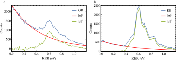
Figure 14: Extraction of $\alpha$ and $\beta$ from the experimental data. a, The blue curve is the KER distribution of the third OB (marked with a solid line in Fig. S8E). b, The blue curve is the KER distribution of the third EB (marked with a dashed line in Fig. S8E). The red curve is and expontential function fitted to the blue curve up to a KER of 0.35 eV giving us $|\alpha|^{2}$. The green curve is obtained by subtracting the red curve from the blue one to get $|\beta|^{2}$.

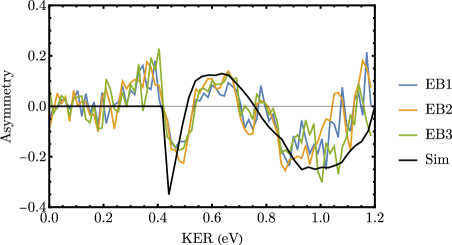
Figure 15: Experimental time-integrated even-band asymmetry parameter as a function of KER. Black curve shows the asymmetry A based on Eq. 38 with $|g_{1}+g_{2}|=\alpha_{e}$ and $|b1|=\beta_{e}$.

The same procedure is repeated for even bands (EBs) where the total number of absorbed photons in each pathway is an even number. According to pathways for even bands shown in Fig. S 10, Eq. 8 becomes

$$\ket{\phi}=(g_{1}+g_{2})\ket{+,+}+b_{1}\ket{-,-}.$$ (36)

The population probability reads

$$P_{even}=|g_{1}+g_{2}+b_{1}|^{2},$$ (37)

and the asymmetry parameter becomes

$$A_{even}(\tau)=\frac{-2(|g_{2}||b_{1}|\cos(\Delta\phi_{g2,b1})+|g_{1}||b_{1}|\cos(\Delta\phi_{g1,b1}))}{|g_{1}|^{2}+|g_{2}|^{2}+|b_{1}|^{2}+2|g_{1}||g_{2}|\cos(\Delta\phi_{b1,b2})},$$ (38)

with complex amplitudes

$$g_{1} = FC_{gs}\mathrm{e}^{\mathrm{i}\theta_{gs}}\times M^{(2)}_{gs},$$ (39)

$$g_{2} = FC_{gs}\mathrm{e}^{\mathrm{i}\theta_{gs}}\times M^{(2)}_{gs},$$ (40)

$$b_{1}=FC_{bs}\mathrm{e}^{\mathrm{i}\theta_{bs}}\times{\color[rgb]{0,0,0}\mathrm{e}^{\mathrm{i}\phi(\tau)}}\times M^{(1)}_{bs}.$$ (41)

The phase difference between the nuclear parts is the same as for the odd bands, $\Delta\Theta_{even}=\Delta\Theta_{odd}$. However, the photo-electron absorbs a different number of IR photons.

The phases of the complex amplitudes are:

$$\mathrm{arg}[g1] =\Theta_{gs}-\frac{\pi\ell}{2}+\phi_{q-2}^{XUV}+\phi(\tau) =\Phi_{g1}+\phi(\tau),$$ (42)

$$\mathrm{arg}[g2] =\Theta_{gs}-\frac{\pi\ell}{2}+\phi_{q}^{XUV}-\phi(\tau) =\Phi_{g2}-\phi(\tau),$$ (43)

$$\mathrm{arg}[b1] =\Theta_{bs}-\frac{\pi}{2}-\frac{\pi\ell}{2}+\phi_{q-2}^{XUV}+\phi(\tau) =\Phi_{b2}+\phi(\tau).$$ (44)

With this, the time dependent asymmetry reads:

$$A_{even}(\tau)=\frac{2|g_{2}||b_{1}|\sin(\Delta\Theta+\Delta\phi_{q,q-2}^{XUV}-2\phi(\tau))+2|g_{1}||b_{1}|\sin(\Delta\Theta)}{|g_{1}|^{2}+|g_{2}|^{2}+|b_{1}|^{2}+2|g_{1}||g_{2}|\cos(\Delta\phi_{q-2,q}^{XUV}+2\phi(\tau))},$$ (45)

and the time-averaged asymmetry parameter is not zero: $\langle A\rangle=\int d\tau A(\tau)\neq 0$.

Fig. 15 shows the experimental time-averaged asymmetry parameter ($\langle A\rangle$) as a function of KER for three odd bands (OBs). They correspond to sidebands 18th (EB1), 20th (EB2), and 22st (EB3). The black line is the theoretical curve (Eq. 45) based on the model explained above.

Figure 16: Even bands: A) and C) Experiment, B) and D) simulation based on the model. A) and B): The asymmetry parameter as a function of the delay between the XUV and IR pulses. Comparison between the experiment and the model based on the WKB approximation shows a good agreement. C) and D): Asymmetry minus the mean time-independent part ($A-\langle A\rangle$). The model here includes only the main three quantum paths that lead to the asymmetry. The values of alpha and beta are obtained using the fit of the experimental data.

The Eq. 2 in the main text is obtained in a similar manner to OBs by writing the final wave function using the defined phases above and their corresponding amplitudes $$\ket{\phi}=(|g_{1}|\mbox{e}^{i(\Phi_{g1}+\phi(\tau))}+|g_{2}|\mbox{e}^{i(\Phi_{g2}-\phi(\tau))})\ket{+,+}+|b_{1}|\mbox{e}^{i(\Phi_{b1}+\phi(\tau))}\ket{-,-}.$$ (46) We neglect pathway $g_{1}$ for the same reasons as explained for the odd bands and get: $$\ket{\phi}=|g_{2}|\mbox{e}^{i(\Phi_{g2}-\phi(\tau))}\ket{+,+}+|b_{1}|\mbox{e}^{i(\Phi_{b1}+\phi(\tau)})\ket{-,-}.$$ (47) By setting $|g_{2}|\mbox{e}^{i\Phi_{g2}}=\alpha_{e}$, $|b_{1}|\mbox{e}^{i\Phi_{b1}}=\beta_{e}$, we get $$\ket{\phi}=\alpha_{e}\ket{+,+}+\beta_{e}\mbox{e}^{i2\phi(\tau)}\ket{-,-}.$$ (48)

3.4.1 Chirp of the XUV pulse

We perform a reference measurement on argon prior to the measurement on H₂. We use the photoelectron spectrum as a function of the delay between XUV and IR pulses (also known as RABBIT spectrum) to retrieve the chirp of the XUV pulse. Fig. S17 shows the relative phase of the different side-bands in the RABBIT spectrum.

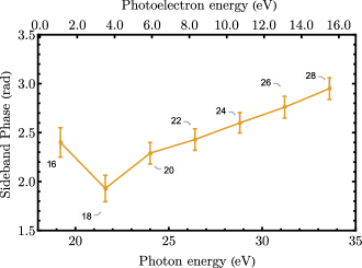
Figure 17: The chirp of the XUV pulses. Shown are the relative phases of the side-bands in photoionization of argon using a combination of XUV and IR pulses. Figure Adapted from [39].

References

- [1] Ryszard Horodecki, Paweł Horodecki, Michał Horodecki, and Karol Horodecki. Quantum entanglement. Rev. Mod. Phys., 81:865–942, Jun 2009.
- [2] M.A. Nielsen and I.L. Chuang. Quantum Computation and Quantum Information: 10th Anniversary Edition. Cambridge University Press, 2010.
- [3] Malte C Tichy, Florian Mintert, and Andreas Buchleitner. Essential entanglement for atomic and molecular physics. Journal of Physics B: Atomic, Molecular and Optical Physics, 44(19):192001, sep 2011.
- [4] Paul G. Kwiat, Klaus Mattle, Harald Weinfurter, Anton Zeilinger, Alexander V. Sergienko, and Yanhua Shih. New high-intensity source of polarization-entangled photon pairs. Phys. Rev. Lett., 75:4337–4341, Dec 1995.
- [5] David C. Burnham and Donald L. Weinberg. Observation of simultaneity in parametric production of optical photon pairs. Phys. Rev. Lett., 25:84–87, Jul 1970.
- [6] Stuart J. Freedman and John F. Clauser. Experimental test of local hidden-variable theories. Phys. Rev. Lett., 28:938–941, Apr 1972.
- [7] M. Lamehi-Rachti and W. Mittig. Quantum mechanics and hidden variables: A test of bell’s inequality by the measurement of the spin correlation in low-energy proton-proton scattering. Phys. Rev. D, 14:2543–2555, Nov 1976.
- [8] E. Hagley, X. Maître, G. Nogues, C. Wunderlich, M. Brune, J. M. Raimond, and S. Haroche. Generation of einstein-podolsky-rosen pairs of atoms. Phys. Rev. Lett., 79:1–5, Jul 1997.
- [9] D. Akoury, K. Kreidi, T. Jahnke, Th. Weber, A. Staudte, M. Schöffler, N. Neumann, J. Titze, L. Ph. H. Schmidt, A. Czasch, O. Jagutzki, R. A. Costa Fraga, R. E. Grisenti, R. Díez Muiño, N. A. Cherepkov, S. K. Semenov, P. Ranitovic, C. L. Cocke, T. Osipov, H. Adaniya, J. C. Thompson, M. H. Prior, A. Belkacem, A. L. Landers, H. Schmidt-Böcking, and R. Dörner. The simplest double slit: Interference and entanglement in double photoionization of h2. Science, 318(5852):949–952, 2007.
- [10] M. S. Schöffler, J. Titze, N. Petridis, T. Jahnke, K. Cole, L. Ph. H. Schmidt, A. Czasch, D. Akoury, O. Jagutzki, J. B. Williams, N. A. Cherepkov, S. K. Semenov, C. W. McCurdy, T. N. Rescigno, C. L. Cocke, T. Osipov, S. Lee, M. H. Prior, A. Belkacem, A. L. Landers, H. Schmidt-Böcking, Th. Weber, and R. Dörner. Ultrafast probing of core hole localization in n2. Science, 320(5878):920–923, 2008.
- [11] F. Martin, J. Fernandez, T. Havermeier, L. Foucar, Th. Weber, K. Kreidi, M. Schoeffler, L. Schmidt, T. Jahnke, O. Jagutzki, A. Czasch, E. P. Benis, T. Osipov, A. L. Landers, A. Belkacem, M. H. Prior, H. Schmidt-Böcking, C. L. Cocke, and R. Doerner. Single photon-induced symmetry breaking of h2 dissociation. Science, 315(5812):629–633, 2007.
- [12] Andrew Steane. Quantum computing. Reports on Progress in Physics, 61(2):117–173, feb 1998.
- [13] Q. A. Turchette, C. S. Wood, B. E. King, C. J. Myatt, D. Leibfried, W. M. Itano, C. Monroe, and D. J. Wineland. Deterministic entanglement of two trapped ions. Phys. Rev. Lett., 81:3631–3634, Oct 1998.
- [14] Rainer Blatt and David Wineland. Entangled states of trapped atomic ions. Nature, 453(7198):1008–1015, Jun 2008.
- [15] Immanuel Bloch. Quantum coherence and entanglement with ultracold atoms in optical lattices. Nature, 453(7198):1016–1022, Jun 2008.
- [16] Morten Kjaergaard, Mollie E. Schwartz, Jochen Braumüller, Philip Krantz, Joel I.-J. Wang, Simon Gustavsson, and William D. Oliver. Superconducting qubits: Current state of play. Annual Review of Condensed Matter Physics, 11(1):369–395, 2020.
- [17] Anasua Chatterjee, Paul Stevenson, Silvano De Franceschi, Andrea Morello, Nathalie P. de Leon, and Ferdinand Kuemmeth. Semiconductor qubits in practice. Nature Reviews Physics, 3(3):157–177, Mar 2021.
- [18] V. M. Schäfer, C. J. Ballance, K. Thirumalai, L. J. Stephenson, T. G. Ballance, A. M. Steane, and D. M. Lucas. Fast quantum logic gates with trapped-ion qubits. Nature, 555(7694):75–78, Mar 2018.
- [19] Yiheng Lin, David R. Leibrandt, Dietrich Leibfried, and Chin-wen Chou. Quantum entanglement between an atom and a molecule. Nature, 581(7808):273–277, May 2020.
- [20] A. Einstein, B. Podolsky, and N. Rosen. Can quantum-mechanical description of physical reality be considered complete? Phys. Rev., 47:777–780, May 1935.
- [21] Ferenc Krausz and Misha Ivanov. Attosecond physics. Rev. Mod. Phys., 81:163–234, Feb 2009.
- [22] Marc J. J. Vrakking. Control of attosecond entanglement and coherence. Phys. Rev. Lett., 126:113203, Mar 2021.
- [23] David Busto, Hugo Laurell, Daniel Finkelstein Shapiro, Christina Alexandridi, Marcus Isinger, Saikat Nandi, Richard Squibb, Margherita Turconi, Shiyang Zhong, Cord Arnold, Raimund Feifel, Mathieu Gisselbrecht, Pascal Salières, Tönu Pullerits, Fernando Martín, Luca Argenti, and Anne L’Huillier. Probing electronic decoherence with high-resolution attosecond photoelectron interferometry, 2021.
- [24] Lisa-Marie Koll, Laura Maikowski, Lorenz Drescher, Tobias Witting, and Marc J. J. Vrakking. Experimental control of quantum-mechanical entanglement in an attosecond pump-probe experiment. Phys. Rev. Lett., 128:043201, Jan 2022.
- [25] Takanori Nishi, Erik Lötstedt, and Kaoru Yamanouchi. Entanglement and coherence in photoionization of by an ultrashort xuv laser pulse. Phys. Rev. A, 100:013421, Jul 2019.
- [26] Marc J J Vrakking. Ion-photoelectron entanglement in photoionization with chirped laser pulses. Journal of Physics B: Atomic, Molecular and Optical Physics, 55(13):134001, jun 2022.
- [27] Mihaela Vatasescu. Entanglement between electronic and vibrational degrees of freedom in a laser-driven molecular system. Phys. Rev. A, 88:063415, Dec 2013.
- [28] Stefanos Carlström, Johan Mauritsson, Kenneth J Schafer, Anne L’Huillier, and Mathieu Gisselbrecht. Quantum coherence in photo-ionisation with tailored XUV pulses. Journal of Physics B: Atomic, Molecular and Optical Physics, 51(1):015201, nov 2017.
- [29] Roger Y. Bello, Fernando Martín, and Alicia Palacios. Attosecond laser control of photoelectron angular distributions in xuv-induced ionization of h2. Faraday discussions, 2021.
- [30] Andreas Fischer, Alexander Sperl, Philipp Cörlin, Michael Schönwald, Helga Rietz, Alicia Palacios, Alberto González-Castrillo, Fernando Martín, Thomas Pfeifer, Joachim Ullrich, Arne Senftleben, and Robert Moshammer. Electron localization involving doubly excited states in broadband extreme ultraviolet ionization of . Phys. Rev. Lett., 110:213002, May 2013.
- [31] Manuel Kremer, Bettina Fischer, Bernold Feuerstein, Vitor L. B. de Jesus, Vandana Sharma, Christian Hofrichter, Artem Rudenko, Uwe Thumm, Claus Dieter Schröter, Robert Moshammer, and Joachim Ullrich. Electron localization in molecular fragmentation of h2 by carrier-envelope phase stabilized laser pulses. Phys. Rev. Lett., 103:213003, Nov 2009.
- [32] G. Sansone, F. Kelkensberg, J. F. Pérez-Torres, F. Morales, M. F. Kling, W. Siu, O. Ghafur, P. Johnsson, M. Swoboda, E. Benedetti, F. Ferrari, F. Lépine, J. L. Sanz-Vicario, S. Zherebtsov, I. Znakovskaya, A. L’Huillier, M. Yu. Ivanov, M. Nisoli, F. Martín, and M. J. J. Vrakking. Electron localization following attosecond molecular photoionization. Nature, 465(7299):763–766, Jun 2010.
- [33] M. F. Kling, Ch. Siedschlag, A. J. Verhoef, J. I. Khan, M. Schultze, Th. Uphues, Y. Ni, M. Uiberacker, M. Drescher, F. Krausz, and M. J. J. Vrakking. Control of electron localization in molecular dissociation. Science, 312(5771):246–248, 2006.
- [34] J Ullrich, R Moshammer, A Dorn, R Dörner, L Ph H Schmidt, and H Schmidt-Böcking. Recoil-ion and electron momentum spectroscopy reaction-microscopes. Reports on Progress in Physics, 66(9):1463, 2003.
- [35] P. M. Paul, E. S. Toma, P. Breger, G. Mullot, F. Augé, Ph. Balcou, H. G. Muller, and P. Agostini. Observation of a train of attosecond pulses from high harmonic generation. Science, 292(5522):1689–1692, 2001.
- [36] L. Cattaneo, J. Vos, R. Y. Bello, A. Palacios, S. Heuser, L. Pedrelli, M. Lucchini, C. Cirelli, F. Martín, and U. Keller. Attosecond coupled electron and nuclear dynamics in dissociative ionization of h2. Nature Physics, 14(7):733–738, Jul 2018.
- [37] P. H. Bucksbaum, A. Zavriyev, H. G. Muller, and D. W. Schumacher. Softening of the molecular bond in intense laser fields. Phys. Rev. Lett., 64:1883–1886, Apr 1990.
- [38] R. Dörner, V. Mergel, O. Jagutzki, L. Spielberger, J. Ullrich, R. Moshammer, and H. Schmidt-Böcking. Cold target recoil ion momentum spectroscopy: a ‘momentum microscope’ to view atomic collision dynamics. Physics Reports, 330(2):95 – 192, 2000.
- [39] Farshad Shobeiry. Attosecond Electron-Nuclear Dynamics in Photodissociation of H2 and D2. PhD thesis, 2021.
- [40] Richard N. Zare. Photoejection dynamics,. Mol. Photochem, 1972.
- [41] Y. M. Chung, E.-M. Lee, T. Masuoka, and James A. R. Samson. Dissociative photoionization of h2 from 18 to 124 ev. The Journal of Chemical Physics, 99(2):885–889, 1993.
- [42] Andreas Fischer, Alexander Sperl, Philipp Cörlin, Michael Schönwald, Sebastian Meuren, Joachim Ullrich, Thomas Pfeifer, Robert Moshammer, and Arne Senftleben. Measurement of the autoionization lifetime of the energetically lowest doubly excited state in h2using electron ejection asymmetry. Journal of Physics B: Atomic, Molecular and Optical Physics, 47(2):021001, dec 2013.
- [43] Alicia Palacios, Johannes Feist, Alberto González-Castrillo, José Luis Sanz-Vicario, and Fernando Martín. Autoionization of molecular hydrogen: Where do the fano lineshapes go? ChemPhysChem, 14(7):1456–1463, 2013.
- [44] Eric E. Aubanel, Jean-Marc Gauthier, and André D. Bandrauk. Molecular stabilization and angular distribution in photodissociation of h2+ in intense laser fields. Phys. Rev. A, 48:2145–2152, Sep 1993.
- [45] Manohar Awasthi, Yulian V. Vanne, Alejandro Saenz, Alberto Castro, and Piero Decleva. Single-active-electron approximation for describing molecules in ultrashort laser pulses and its application to molecular hydrogen. Phys. Rev. A, 77:063403, Jun 2008.
- [46] Divya Bharti, David Atri-Schuller, Gavin Menning, Kathryn R. Hamilton, Robert Moshammer, Thomas Pfeifer, Nicolas Douguet, Klaus Bartschat, and Anne Harth. Decomposition of the transition phase in multi-sideband schemes for reconstruction of attosecond beating by interference of two-photon transitions. Phys. Rev. A, 103:022834, Feb 2021.
- [47] H.G. Muller. Reconstruction of attosecond harmonic beating by interference of two-photon transitions. Applied Physics B, 74(1):s17–s21, 2002.