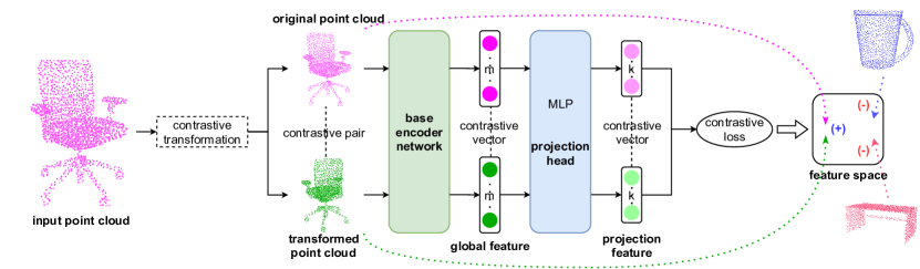
L = − 1 S ∑ ( i , j ) ∈ S log exp ( 𝐳 𝐢 ⋅ 𝐳 𝐣 / τ ) ∑ ( ⋅ , t ) ∈ S , t ≠ j exp ( 𝐳 𝐢 ⋅ 𝐳 𝐭 / τ ) , w h e r e S i s t h e s e t o f a l l p o s i t i v e p a i r s ( p o i n t c l o u d l e v e l ) , a n d τ i s a t e m p e r a t u r e p a r a m e t e r . d e n o t e s t h e c a r d i n a l i t y o f t h e s e t . T h e l o s s i s c o m p u t e d u s i n g a l l t h e c o n t r a s t i v e p a i r s , a n d i s e q u i v a l e n t t o a p p l y i n g t h e c r o s s e n t r o p y w i t h p s e u d o l a b e l s ( e . g . 0∼15 f o r 16 p a i r s ) . W e f o u n d i t w o r k s v e r y w e l l i n o u r u n s u p e r v i s e d c o n t r a s t i v e r e p r e s e n t a t i o n l e a r n i n g .
3.2 Downstream 3D Object Classification
We take 3D object classification as the first downstream task in this work, to validate our unsupervised representation learning. The above designed scheme is immediately ready for the unsupervised representation learning to facilitate the downstream classification task.
In particular, we will utilize two common schemes for validation here. One is to train a linear classification network by taking the learned representations of our unsupervised learning as input. Here, the learned representation is the global feature. We did not choose the k 4.6 4
3.3 Downstream Semantic Segmentation
To further demonstrate the effectiveness of our unsupervised representation learning, we also fit the above unsupervised learning scheme to the downstream semantic segmentation, including shape part segmentation and scene segmentation.
Since it is a different task from 3D object classification, we need to design a new scheme to facilitate unsupervised training. We still use the rotation to generate a transformed version of an original point cloud (e.g. a shape point cloud or a split block from the scene), and view them as a contrastive pair (i.e. point cloud level). As for segmentation, each point in the point cloud has a feature representation. For unsupervised representation learning, we compute the mean of all point-wise cross entropy to evaluate the overall similarity within the mini-batch.
We therefore define a loss function for semantic segmentation as:
= L - 1 S ∑ ∈ ( a , b ) S 1 P ( a , b ) ∑ ∈ ( i , j ) P ( a , b ) (3)
log exp ( / ⋅ z i z j τ ) ∑ ∈ ( ⋅ , t ) P ( a , b ) , ≠ t j exp ( / ⋅ z i z t τ ) ,
where S a b P ( a , b ) a b ∼ 0 2047
4 Experimental Results
Table 1: Classification results of unsupervised methods and our method (Linear Classifier), on the datasets of ModelNet40 and ModelNet10. Both ShapeNet55 (upper part) and ModelNet40 (bottom part) pretrained datasets are provided.
4.1 Datasets
Object classification.
We utilize ModelNet40 and ModelNet10 wu20153d qi2017pointnet ; qi2017pointnet++ ; wang2019dynamic 9 , 840 2 , 468 3 , 991 1 , 024 ( x , y , z )
We provide comparison experiments with PointContrast xie2020pointcontrast chang2015shapenet 51 , 127 35 , 708 5 , 158 10 , 261 1 , 024 xie2020pointcontrast
Shape part segmentation.
We use the ShapeNet Part dataset yi2016scalable 16 , 881 chang2015shapenet qi2017pointnet++ ; wang2019dynamic
Scene segmentation.
We also evaluate our model for scene segmentation on Stanford Large-Scale 3D Indoor Spaces Dataset (S3DIS) armeni2017joint 6 , 000 m 2 qi2017pointnet++ ; wang2019dynamic × 1 m 1 m 4 , 096
Please refer to the Appendices for additional information and visual results.
4.2 Experimental Setting
We use Adam optimizer for our unsupervised representation training. We implemented our work with TensorFlow, and use a single TITAN V GPU for training (DGCNN using multiple GPUs).
For downstream 3D object classification on ModelNet40, ModelNet10, ShapeNet55 and ShapeNetCore , we use a batch size of 32 (i.e. 16 contrastive pairs) for training and testing. Temperature hyper-parameter τ
We employ DGCNN as the backbone for semantic segmentation. As for shape part segmentation on ShapeNet Part dataset, we utilize a batch size of 16 (i.e. 8 constrasive pairs) for training. We use a batch size of 12 (i.e. 6 constrasive pairs) for scene segmentation on S3DIS. For the two tasks, we simply use a batch size of 1 during testing, and the other settings follow DGCNN.
4.3 3D Object Classification
We conduct two kinds of experiments to evaluate the learned representations of our unsupervised contrastive learning. We first train a simple linear classification network with the unsupervised representations as input. Secondly, we take our unsupervised representation learning as pretraining, and initialize the weights of the backbone before supervised training. Tables 1 3
Linear classification evaluation.
In this part, we use the former part of PointNet qi2017pointnet wang2019dynamic 1 % 95.09 % 90.64 % 90.32 % 88.65 Our method with DGCNN as backbone also outperforms most unsupervised techniques, like two recent methods PointHop (% 1.22 % 0.17 3 % 90.32 % 90.6 % 90.9 % 95.09 % 93.9 The GLR rao2020global × liu2019relation
Notice that some methods used a larger ShapeNet55 dataset for training yang2018foldingnet ; gadelha2018multiresolution ; achlioptas2018learning ; zhao20193d han2019multi zhao20193d 1 % 2.86
To show our learned representations have the transfer capability, we also train our method (DGCNN as backbone) on ShapeNet55 dataset for unsupervised contrastive learning and then feed the ModelNet40 dataset to the trained model to get point cloud features. We use these features to train a linear classifier on ModelNet40 for evaluation. From Table 1 achlioptas2018learning yang2018foldingnet zhao20193d % 3.67 % 0.97 % 0.47
We also conduct an experiment for training with limited data to verify the capability of our pretrained model with linear classifier. The results can be seen in Table 2 % 86.6 % 30 % 2.4 yang2018foldingnet % 84.2 % 10 % 0.6
Table 2: Comparison results of classification accuracy with limited training data (different ratios).
Table 3: Classification results of other supervised methods and our method (Pretraining), on the datasets of ModelNet40 and ModelNet10. We distinguish the results of other methods from our method by the line.
Pretraining evaluation. In addition to the above evaluation using a linear classifier, we further utilize the pre-training evaluation to demonstrate the efficacy of our unsupervised contrastive representation learning. Specifically, we also select PointNet and DGCNN as the backbone, in which the part before and including the global feature is regarded as the base encoder, and the remaining classification branch (i.e. several mlp layers) as the projection head. After our unsupervised representation training, we initialize the corresponding network with the unsupervised trained model, and then perform the supervised training. Table 3
The pretraining evaluation based on our unsupervised representation learning sees an improvement over the original backbone network, increased from % 89.2 % 90.44 % 1.24 % 92.2 % 93.03 % 0.83 Regarding ModelNet10, the accuracy of PointNet as our backbone for pretraining evaluation is % 94.38 % 93.9 fujiwara2020neural yan2020pointasnl fujiwara2020neural % 93.03 lin2020convolution fujiwara2020neural yan2020pointasnl
Compared to using PointNet as backbone, taking DGCNN as backbone achieves a better classification accuracy, for example, % 95.93 % 94.38 % 93.03 % 90.44
PointContrast xie2020pointcontrast 4 % 0.5 wang2019dynamic % 84.0 % 86.2 % 0.6 % 2.2
Table 4: Comparison results of PointContrast and our method on the dataset of ShapeNetCore with Pretraining evaluation. Note that * represents that the model is trained on ScanNet.
4.4 Shape Part Segmentation
In addition to the 3D object classification, we also verify our method on shape part segmentation.
The segmentation results are listed in Table 5 % 79.2 % 75.5 han2019multi hassani2019unsupervised han2019multi hassani2019unsupervised % 7.55 % 3.4 2
Table 5: Shape part segmentation results of our method (Linear Classifier) and state-of-the-art techniques on ShapeNet Part dataset. We distinguish between supervised and unsupervised learning methods by the line.
Figure 2: Some examples of shape part segmentation using our method (Linear Classifier setting).
4.5 Scene Segmentation
We also test our method for the scene segmentation task on the S3DIS dataset, which typically appears to be more challenging than the shape part segmentation. Similarly, we utilize DGCNN as the backbone and adopt the Linear Classifier evaluation setting.
We are not able to compare our method with unsupervised methods like MAP-VAE han2019multi hassani2019unsupervised 6 3
Table 6: Scene segmentation results of our method (Linear Classifier) and some state-of-the-art techniques on testing Area 5 (Fold 1) of the S3DIS dataset.
Figure 3: Visual result of scene segmentation.
4.6 Ablation Studies
Transformation.
One of the key elements in our unsupervised representation learning is using 180 ∘ Y 4
We list the comparison results of the above transformations in Table 7 chen2020simple 180 ∘ Y
Furthermore, we apply two sequential transformations on one point cloud and make the result as a pair with the original point cloud. We chose the best transformation (i.e. rotate 180 ∘ Y 8
Figure 4: Illustration for transformations used in Table 7
Table 7: Comparison of different contrastive transformation on ModelNet10. DGCNN wang2019dynamic
Table 8: Comparison of more complex contrastive transformation on ModelNet10. We distinguish between the results of using only two transformations and those of using four transformations (more complex) by the line. “Rotate” means 180 ∘ Y wang2019dynamic
Output of encoder versus output of projection head.
We also compare the choices of using the output of the base encoder (i.e. global feature) and the output of the projection head for subsequent linear classification. Table 9
Table 9: Comparison of using the output of encoder and projection head for linear classification evaluation. PointNet qi2017pointnet
Cross validation.
In addition to the above evaluations, we further test the abilities of our unsupervised contrastive representation learning in a crossed evaluation setting. To achieve this, we use the learned representations from the unsupervised trained model on ModelNet40 to further train a linear classifier on ModelNet10, and vice versa. Classification outcomes are reported in Table 10
Table 10: Cross validation for ModelNet40 and ModelNet10. We perform unsupervised learning on one dataset and conduct the classification task on another dataset. PointNet qi2017pointnet
Pretraining evaluation: initializing projection head.
Projection head is very useful in maximizing the agreement between the contrastive pair. However, it may hinder pretraining evaluation, if the corresponding part is initialized with the projection head of the unsupervised model. Table 11
Table 11: Pretraining validation to determine whether using preojection head for initialization. ModelNet40 and ModelNet10 are used for datasets. PointNet qi2017pointnet wang2019dynamic
T-SNE Visualization.
We utilize the t-SNE to visualize the features learned on ModelNet40 in Figure 5
Figure 5: T-SNE visualization of features. (a) without contrastive learning, (b) with contrastive learning.
5 Conclusion
We have presented an unsupervised representation learning method for 3D point cloud data. We identified that rotation is a very useful transformation for generating a contrastive version of an original point cloud. Unsupervised representations are learned via maximizing the correspondence between paired point clouds (i.e. an original point cloud and its contrastive version). Our method is simple to implement and does not require expensive computing resources like TPU. We evaluate our unsupervised representations for the downstream tasks including 3D object classification, shape part segmentation and scene segmentation. Experimental results demonstrate that our method generates impressive performance. In the future, We would like to exploit semi-supervised techniques like feng2020dmt
Conflicts of Interests
The authors declare that the work is original and has not been submitted elsewhere.
Appendix A Overview of Segmentation
Figure 6: Overview of our unsupervised contrastive learning for the downstream segmentation task. All the point clouds in the minibatch will be mapped into the feature space. The designed contrastive loss (shown in the main paper) encourages a pair of point clouds (original point cloud and its transformed point cloud) to be consistent in the feature space, and the point-wise features of the same point ID also tend to be consistent.
We also achieve the task of point cloud semantic segmentation, including shape part segmentation and scene segmentation. Different from the 3D object classification task, we need to gain all the point-wise features in the point cloud, which is the key to solve the segmentation task. For our unsupervised contrastive learning, as shown in Figure 6 , we still consider the original point cloud and its transformed point cloud as a contrastive pair. However, in order to ensure that the feature of each point in the point cloud will be learned, we use the mean of point-wise cross entropy to evaluate the point cloud similarity, and try to maximize the similarity of the positive pair (all other pairs of point clouds in the minibatch are viewed as negative pairs). In this unsupervised manner, our framework can learn the feature of each point in the point cloud.
Appendix B Additional Visual Results on Scene Segmentation
In this section, we show more visual results on scene segmentation. Similarly, we utilize the Linear Classifier setting for this downstream task. Figure 7
Figure 7: Visual result of scene segmentation.
Appendix C Additional Visual Results on Shape Part Segmentation
In this section, we put more visual results of our method on the downstream shape part segmentation. We simply employ the Linear Classifier setting for this downstream task. Figure 8
Figure 8: Some examples of all 16 categories in ShapeNet Part dataset.
References
\bibcommenthead
(1)
Wu, Z.,
Song, S.,
Khosla, A.,
Yu, F.,
Zhang, L.,
Tang, X.,
Xiao, J.:
3d shapenets: A deep representation for volumetric shapes.
In: Proceedings of the IEEE Conference on Computer Vision and Pattern
Recognition,
pp. 1912–1920
(2015)
(2)
Riegler, G.,
Osman Ulusoy, A.,
Geiger, A.:
Octnet: Learning deep 3d representations at high resolutions.
In: Proceedings of the IEEE Conference on Computer Vision and Pattern
Recognition,
pp. 3577–3586
(2017)
(3)
Wang, P.-S.,
Liu, Y.,
Guo, Y.-X.,
Sun, C.-Y.,
Tong, X.:
O-cnn: Octree-based convolutional neural networks for 3d shape
analysis.
ACM Transactions on Graphics (TOG)
36 (4),
1–11
(2017)
(4)
Su, H.,
Maji, S.,
Kalogerakis, E.,
Learned-Miller, E.:
Multi-view convolutional neural networks for 3d shape recognition.
In: Proceedings of the IEEE International Conference on Computer
Vision,
pp. 945–953
(2015)
(5)
Li, L.,
Zhu, S.,
Fu, H.,
Tan, P.,
Tai, C.-L.:
End-to-end learning local multi-view descriptors for 3d point clouds.
In: Proceedings of the IEEE/CVF Conference on Computer Vision and
Pattern Recognition,
pp. 1919–1928
(2020)
(6)
Lyu, Y.,
Huang, X.,
Zhang, Z.:
Learning to segment 3d point clouds in 2d image space.
In: Proceedings of the IEEE/CVF Conference on Computer Vision and
Pattern Recognition,
pp. 12255–12264
(2020)
(7)
Qi, C.R.,
Su, H.,
Mo, K.,
Guibas, L.J.:
Pointnet: Deep learning on point sets for 3d classification and
segmentation.
In: Proceedings of the IEEE Conference on Computer Vision and Pattern
Recognition,
pp. 652–660
(2017)
(8)
Qi, C.R.,
Yi, L.,
Su, H.,
Guibas, L.J.:
Pointnet++: Deep hierarchical feature learning on point sets in a
metric space.
In: Advances in Neural Information Processing Systems,
pp. 5099–5108
(2017)
(9)
Li, Y.,
Bu, R.,
Sun, M.,
Wu, W.,
Di, X.,
Chen, B.:
Pointcnn: Convolution on x-transformed points.
In: Advances in Neural Information Processing Systems,
pp. 820–830
(2018)
(10)
Achlioptas, P.,
Diamanti, O.,
Mitliagkas, I.,
Guibas, L.:
Learning representations and generative models for 3d point clouds.
In: International Conference on Machine Learning,
pp. 40–49
(2018).
PMLR
(11)
Yang, Y.,
Feng, C.,
Shen, Y.,
Tian, D.:
Foldingnet: Point cloud auto-encoder via deep grid deformation.
In: Proceedings of the IEEE Conference on Computer Vision and Pattern
Recognition,
pp. 206–215
(2018)
(12)
Han, Z.,
Wang, X.,
Liu, Y.-S.,
Zwicker, M.:
Multi-angle point cloud-vae: unsupervised feature learning for 3d
point clouds from multiple angles by joint self-reconstruction and
half-to-half prediction.
In: 2019 IEEE/CVF International Conference on Computer Vision (ICCV),
pp. 10441–10450
(2019).
IEEE
(13)
Zhao, Y.,
Birdal, T.,
Deng, H.,
Tombari, F.:
3d point capsule networks.
In: Proceedings of the IEEE Conference on Computer Vision and Pattern
Recognition,
pp. 1009–1018
(2019)
(14)
Zhang, D.,
Lu, X.,
Qin, H.,
He, Y.:
Pointfilter: Point cloud filtering via encoder-decoder modeling.
IEEE Transactions on Visualization and Computer Graphics,
1–1
(2020).
https://doi.org/10.1109/TVCG.2020.3027069
(15)
Lu, D.,
Lu, X.,
Sun, Y.,
Wang, J.:
Deep feature-preserving normal estimation for point cloud filtering.
Computer-Aided Design
125 ,
102860
(2020).
https://doi.org/10.1016/j.cad.2020.102860
(16)
Lu, X.,
Schaefer, S.,
Luo, J.,
Ma, L.,
He, Y.:
Low rank matrix approximation for 3d geometry filtering.
IEEE Transactions on Visualization and Computer Graphics,
1–1
(2020).
https://doi.org/10.1109/TVCG.2020.3026785
(17)
Lu, X.,
Wu, S.,
Chen, H.,
Yeung, S.,
Chen, W.,
Zwicker, M.:
Gpf: Gmm-inspired feature-preserving point set filtering.
IEEE Transactions on Visualization and Computer Graphics
24 (8),
2315–2326
(2018).
https://doi.org/10.1109/TVCG.2017.2725948
(18)
Su, H.,
Jampani, V.,
Sun, D.,
Maji, S.,
Kalogerakis, E.,
Yang, M.-H.,
Kautz, J.:
Splatnet: Sparse lattice networks for point cloud processing.
In: Proceedings of the IEEE Conference on Computer Vision and Pattern
Recognition,
pp. 2530–2539
(2018)
(19)
Zhou, H.-Y.,
Liu, A.-A.,
Nie, W.-Z.,
Nie, J.:
Multi-view saliency guided deep neural network for 3-d object
retrieval and classification.
IEEE Transactions on Multimedia
22 (6),
1496–1506
(2019)
(20)
Wu, W.,
Qi, Z.,
Fuxin, L.:
Pointconv: Deep convolutional networks on 3d point clouds.
In: Proceedings of the IEEE Conference on Computer Vision and Pattern
Recognition,
pp. 9621–9630
(2019)
(21)
Xu, Y.,
Fan, T.,
Xu, M.,
Zeng, L.,
Qiao, Y.:
Spidercnn: Deep learning on point sets with parameterized
convolutional filters.
In: Proceedings of the European Conference on Computer Vision (ECCV),
pp. 87–102
(2018)
(22)
Liu, Y.,
Fan, B.,
Xiang, S.,
Pan, C.:
Relation-shape convolutional neural network for point cloud analysis.
In: Proceedings of the IEEE Conference on Computer Vision and Pattern
Recognition,
pp. 8895–8904
(2019)
(23)
Komarichev, A.,
Zhong, Z.,
Hua, J.:
A-cnn: Annularly convolutional neural networks on point clouds.
In: Proceedings of the IEEE Conference on Computer Vision and Pattern
Recognition,
pp. 7421–7430
(2019)
(24)
Wang, Y.,
Sun, Y.,
Liu, Z.,
Sarma, S.E.,
Bronstein, M.M.,
Solomon, J.M.:
Dynamic graph cnn for learning on point clouds.
Acm Transactions On Graphics (tog)
38 (5),
1–12
(2019)
(25)
Lin, Z.-H.,
Huang, S.-Y.,
Wang, Y.-C.F.:
Convolution in the cloud: Learning deformable kernels in 3d graph
convolution networks for point cloud analysis.
In: Proceedings of the IEEE/CVF Conference on Computer Vision and
Pattern Recognition,
pp. 1800–1809
(2020)
(26)
Jiang, L.,
Shi, S.,
Tian, Z.,
Lai, X.,
Liu, S.,
Fu, C.-W.,
Jia, J.:
Guided point contrastive learning for semi-supervised point cloud
semantic segmentation.
In: Proceedings of the IEEE/CVF International Conference on Computer
Vision,
pp. 6423–6432
(2021)
(27)
Du, B.,
Gao, X.,
Hu, W.,
Li, X.:
Self-contrastive learning with hard negative sampling for
self-supervised point cloud learning.
In: Proceedings of the 29th ACM International Conference on
Multimedia,
pp. 3133–3142
(2021)
(28)
Xu, C.,
Leng, B.,
Chen, B.,
Zhang, C.,
Zhou, X.:
Learning discriminative and generative shape embeddings for
three-dimensional shape retrieval.
IEEE Transactions on Multimedia
22 (9),
2234–2245
(2019)
(29)
Huang, J.,
Yan, W.,
Li, T.H.,
Liu, S.,
Li, G.:
Learning the global descriptor for 3d object recognition based on multiple
views decomposition.
IEEE Transactions on Multimedia
(2020)
(30)
Simonovsky, M.,
Komodakis, N.:
Dynamic edge-conditioned filters in convolutional neural networks on
graphs.
In: Proceedings of the IEEE Conference on Computer Vision and Pattern
Recognition,
pp. 3693–3702
(2017)
(31)
Wang, S.,
Suo, S.,
Ma, W.-C.,
Pokrovsky, A.,
Urtasun, R.:
Deep parametric continuous convolutional neural networks.
In: Proceedings of the IEEE Conference on Computer Vision and Pattern
Recognition,
pp. 2589–2597
(2018)
(32)
Li, J.,
Chen, B.M.,
Hee Lee, G.:
So-net: Self-organizing network for point cloud analysis.
In: Proceedings of the IEEE Conference on Computer Vision and Pattern
Recognition,
pp. 9397–9406
(2018)
(33)
Zhao, H.,
Jiang, L.,
Fu, C.-W.,
Jia, J.:
Pointweb: Enhancing local neighborhood features for point cloud
processing.
In: Proceedings of the IEEE Conference on Computer Vision and Pattern
Recognition,
pp. 5565–5573
(2019)
(34)
Xie, S.,
Liu, S.,
Chen, Z.,
Tu, Z.:
Attentional shapecontextnet for point cloud recognition.
In: Proceedings of the IEEE Conference on Computer Vision and Pattern
Recognition,
pp. 4606–4615
(2018)
(35)
Fujiwara, K.,
Hashimoto, T.:
Neural implicit embedding for point cloud analysis.
In: Proceedings of the IEEE/CVF Conference on Computer Vision and
Pattern Recognition,
pp. 11734–11743
(2020)
(36)
Yan, X.,
Zheng, C.,
Li, Z.,
Wang, S.,
Cui, S.:
Pointasnl: Robust point clouds processing using nonlocal neural
networks with adaptive sampling.
In: Proceedings of the IEEE/CVF Conference on Computer Vision and
Pattern Recognition,
pp. 5589–5598
(2020)
(37)
Qiu, S.,
Anwar, S.,
Barnes, N.:
Geometric back-projection network for point cloud classification.
IEEE Transactions on Multimedia
(2021)
(38)
Chen, C.,
Qian, S.,
Fang, Q.,
Xu, C.:
Hapgn: Hierarchical attentive pooling graph network for point cloud
segmentation.
IEEE Transactions on Multimedia
(2020)
(39)
Liu, H.,
Guo, Y.,
Ma, Y.,
Lei, Y.,
Wen, G.:
Semantic context encoding for accurate 3d point cloud segmentation.
IEEE Transactions on Multimedia
(2020)
(40)
Rao, Y.,
Lu, J.,
Zhou, J.:
Global-local bidirectional reasoning for unsupervised representation
learning of 3d point clouds.
In: Proceedings of the IEEE/CVF Conference on Computer Vision and
Pattern Recognition,
pp. 5376–5385
(2020)
(41)
Zhang, M.,
You, H.,
Kadam, P.,
Liu, S.,
Kuo, C.-C.J.:
Pointhop: An explainable machine learning method for point cloud
classification.
IEEE Transactions on Multimedia
22 (7),
1744–1755
(2020)
(42)
Xie, S.,
Gu, J.,
Guo, D.,
Qi, C.R.,
Guibas, L.,
Litany, O.:
Pointcontrast: Unsupervised pre-training for 3d point cloud
understanding.
In: European Conference on Computer Vision,
pp. 574–591
(2020).
Springer
(43)
Chen, T.,
Kornblith, S.,
Norouzi, M.,
Hinton, G.:
A simple framework for contrastive learning of visual
representations.
In: International Conference on Machine Learning,
pp. 1597–1607
(2020).
PMLR
(44)
Oord, A.v.d.,
Li, Y.,
Vinyals, O.:
Representation learning with contrastive predictive coding.
arXiv preprint arXiv:1807.03748
(2018)
(45)
Gadelha, M.,
Wang, R.,
Maji, S.:
Multiresolution tree networks for 3d point cloud processing.
In: Proceedings of the European Conference on Computer Vision (ECCV),
pp. 103–118
(2018)
(46)
Han, Z.,
Shang, M.,
Liu, Y.-S.,
Zwicker, M.:
View inter-prediction gan: Unsupervised representation learning for 3d
shapes by learning global shape memories to support local view predictions.
In: Proceedings of the AAAI Conference on Artificial Intelligence,
vol. 33,
pp. 8376–8384
(2019)
(47)
Chang, A.X.,
Funkhouser, T.,
Guibas, L.,
Hanrahan, P.,
Huang, Q.,
Li, Z.,
Savarese, S.,
Savva, M.,
Song, S.,
Su, H., et al.:
Shapenet: An information-rich 3d model repository.
arXiv preprint arXiv:1512.03012
(2015)
(48)
Yi, L.,
Kim, V.G.,
Ceylan, D.,
Shen, I.-C.,
Yan, M.,
Su, H.,
Lu, C.,
Huang, Q.,
Sheffer, A.,
Guibas, L.:
A scalable active framework for region annotation in 3d shape
collections.
ACM Transactions on Graphics (ToG)
35 (6),
1–12
(2016)
(49)
Armeni, I.,
Sax, S.,
Zamir, A.R.,
Savarese, S.:
Joint 2d-3d-semantic data for indoor scene understanding.
arXiv preprint arXiv:1702.01105
(2017)
(50)
Klokov, R.,
Lempitsky, V.:
Escape from cells: Deep kd-networks for the recognition of 3d point
cloud models.
In: Proceedings of the IEEE International Conference on Computer
Vision,
pp. 863–872
(2017)
(51)
Shen, Y.,
Feng, C.,
Yang, Y.,
Tian, D.:
Mining point cloud local structures by kernel correlation and graph
pooling.
In: Proceedings of the IEEE Conference on Computer Vision and Pattern
Recognition,
pp. 4548–4557
(2018)
(52)
Thomas, H.,
Qi, C.R.,
Deschaud, J.-E.,
Marcotegui, B.,
Goulette, F.,
Guibas, L.J.:
Kpconv: Flexible and deformable convolution for point clouds.
In: Proceedings of the IEEE International Conference on Computer
Vision,
pp. 6411–6420
(2019)
(53)
Atzmon, M.,
Maron, H.,
Lipman, Y.:
Point convolutional neural networks by extension operators.
ACM Transactions on Graphics (TOG)
37 (4),
1–12
(2018)
(54)
Liu, X.,
Han, Z.,
Liu, Y.-S.,
Zwicker, M.:
Point2sequence: Learning the shape representation of 3d point clouds
with an attention-based sequence to sequence network.
In: Proceedings of the AAAI Conference on Artificial Intelligence,
vol. 33,
pp. 8778–8785
(2019)
(55)
Hassani, K.,
Haley, M.:
Unsupervised multi-task feature learning on point clouds.
In: Proceedings of the IEEE International Conference on Computer
Vision,
pp. 8160–8171
(2019)
(56)
Huang, Q.,
Wang, W.,
Neumann, U.:
Recurrent slice networks for 3d segmentation of point clouds.
In: Proceedings of the IEEE Conference on Computer Vision and Pattern
Recognition,
pp. 2626–2635
(2018)
(57)
Feng, Z.,
Zhou, Q.,
Gu, Q.,
Tan, X.,
Cheng, G.,
Lu, X.,
Shi, J.,
Ma, L.:
Dmt: Dynamic mutual training for semi-supervised learning.
arXiv preprint arXiv:2004.08514
(2020)
formulae-sequence 𝐿 1 S subscript 𝑖 𝑗 𝑆 ⋅ subscript 𝐳 𝐢 subscript 𝐳 𝐣 𝜏 subscript formulae-sequence ⋅ 𝑡 𝑆 𝑡 𝑗 ⋅ subscript 𝐳 𝐢 subscript 𝐳 𝐭 𝜏 𝑤 ℎ 𝑒 𝑟 𝑒 𝑆 𝑖 𝑠 𝑡 ℎ 𝑒 𝑠 𝑒 𝑡 𝑜 𝑓 𝑎 𝑙 𝑙 𝑝 𝑜 𝑠 𝑖 𝑡 𝑖 𝑣 𝑒 𝑝 𝑎 𝑖 𝑟 𝑠 𝑝 𝑜 𝑖 𝑛 𝑡 𝑐 𝑙 𝑜 𝑢 𝑑 𝑙 𝑒 𝑣 𝑒 𝑙 𝑎 𝑛 𝑑 𝜏 𝑖 𝑠 𝑎 𝑡 𝑒 𝑚 𝑝 𝑒 𝑟 𝑎 𝑡 𝑢 𝑟 𝑒 𝑝 𝑎 𝑟 𝑎 𝑚 𝑒 𝑡 𝑒 𝑟
d e n o t e s t h e c a r d i n a l i t y o f t h e s e t . T h e l o s s i s c o m p u t e d u s i n g a l l t h e c o n t r a s t i v e p a i r s , a n d i s e q u i v a l e n t t o a p p l y i n g t h e c r o s s e n t r o p y w i t h p s e u d o l a b e l s ( e . g . 0∼15 f o r 16 p a i r s ) . W e f o u n d i t w o r k s v e r y w e l l i n o u r u n s u p e r v i s e d c o n t r a s t i v e r e p r e s e n t a t i o n l e a r n i n g .
3.2 Downstream 3D Object Classification
We take 3D object classification as the first downstream task in this work, to validate our unsupervised representation learning. The above designed scheme is immediately ready for the unsupervised representation learning to facilitate the downstream classification task.
In particular, we will utilize two common schemes for validation here. One is to train a linear classification network by taking the learned representations of our unsupervised learning as input. Here, the learned representation is the global feature. We did not choose the k 4.6 4
3.3 Downstream Semantic Segmentation
To further demonstrate the effectiveness of our unsupervised representation learning, we also fit the above unsupervised learning scheme to the downstream semantic segmentation, including shape part segmentation and scene segmentation.
Since it is a different task from 3D object classification, we need to design a new scheme to facilitate unsupervised training. We still use the rotation to generate a transformed version of an original point cloud (e.g. a shape point cloud or a split block from the scene), and view them as a contrastive pair (i.e. point cloud level). As for segmentation, each point in the point cloud has a feature representation. For unsupervised representation learning, we compute the mean of all point-wise cross entropy to evaluate the overall similarity within the mini-batch.
We therefore define a loss function for semantic segmentation as:
= L - 1 S ∑ ∈ ( a , b ) S 1 P ( a , b ) ∑ ∈ ( i , j ) P ( a , b ) (3)
log exp ( / ⋅ z i z j τ ) ∑ ∈ ( ⋅ , t ) P ( a , b ) , ≠ t j exp ( / ⋅ z i z t τ ) ,
where S a b P ( a , b ) a b ∼ 0 2047
4 Experimental Results
Table 1: Classification results of unsupervised methods and our method (Linear Classifier), on the datasets of ModelNet40 and ModelNet10. Both ShapeNet55 (upper part) and ModelNet40 (bottom part) pretrained datasets are provided.
4.1 Datasets
Object classification.
We utilize ModelNet40 and ModelNet10 wu20153d qi2017pointnet ; qi2017pointnet++ ; wang2019dynamic 9 , 840 2 , 468 3 , 991 1 , 024 ( x , y , z )
We provide comparison experiments with PointContrast xie2020pointcontrast chang2015shapenet 51 , 127 35 , 708 5 , 158 10 , 261 1 , 024 xie2020pointcontrast
Shape part segmentation.
We use the ShapeNet Part dataset yi2016scalable 16 , 881 chang2015shapenet qi2017pointnet++ ; wang2019dynamic
Scene segmentation.
We also evaluate our model for scene segmentation on Stanford Large-Scale 3D Indoor Spaces Dataset (S3DIS) armeni2017joint 6 , 000 m 2 qi2017pointnet++ ; wang2019dynamic × 1 m 1 m 4 , 096
Please refer to the Appendices for additional information and visual results.
4.2 Experimental Setting
We use Adam optimizer for our unsupervised representation training. We implemented our work with TensorFlow, and use a single TITAN V GPU for training (DGCNN using multiple GPUs).
For downstream 3D object classification on ModelNet40, ModelNet10, ShapeNet55 and ShapeNetCore , we use a batch size of 32 (i.e. 16 contrastive pairs) for training and testing. Temperature hyper-parameter τ
We employ DGCNN as the backbone for semantic segmentation. As for shape part segmentation on ShapeNet Part dataset, we utilize a batch size of 16 (i.e. 8 constrasive pairs) for training. We use a batch size of 12 (i.e. 6 constrasive pairs) for scene segmentation on S3DIS. For the two tasks, we simply use a batch size of 1 during testing, and the other settings follow DGCNN.
4.3 3D Object Classification
We conduct two kinds of experiments to evaluate the learned representations of our unsupervised contrastive learning. We first train a simple linear classification network with the unsupervised representations as input. Secondly, we take our unsupervised representation learning as pretraining, and initialize the weights of the backbone before supervised training. Tables 1 3
Linear classification evaluation.
In this part, we use the former part of PointNet qi2017pointnet wang2019dynamic 1 % 95.09 % 90.64 % 90.32 % 88.65 Our method with DGCNN as backbone also outperforms most unsupervised techniques, like two recent methods PointHop (% 1.22 % 0.17 3 % 90.32 % 90.6 % 90.9 % 95.09 % 93.9 The GLR rao2020global × liu2019relation
Notice that some methods used a larger ShapeNet55 dataset for training yang2018foldingnet ; gadelha2018multiresolution ; achlioptas2018learning ; zhao20193d han2019multi zhao20193d 1 % 2.86
To show our learned representations have the transfer capability, we also train our method (DGCNN as backbone) on ShapeNet55 dataset for unsupervised contrastive learning and then feed the ModelNet40 dataset to the trained model to get point cloud features. We use these features to train a linear classifier on ModelNet40 for evaluation. From Table 1 achlioptas2018learning yang2018foldingnet zhao20193d % 3.67 % 0.97 % 0.47
We also conduct an experiment for training with limited data to verify the capability of our pretrained model with linear classifier. The results can be seen in Table 2 % 86.6 % 30 % 2.4 yang2018foldingnet % 84.2 % 10 % 0.6
Table 2: Comparison results of classification accuracy with limited training data (different ratios).
Table 3: Classification results of other supervised methods and our method (Pretraining), on the datasets of ModelNet40 and ModelNet10. We distinguish the results of other methods from our method by the line.
Pretraining evaluation. In addition to the above evaluation using a linear classifier, we further utilize the pre-training evaluation to demonstrate the efficacy of our unsupervised contrastive representation learning. Specifically, we also select PointNet and DGCNN as the backbone, in which the part before and including the global feature is regarded as the base encoder, and the remaining classification branch (i.e. several mlp layers) as the projection head. After our unsupervised representation training, we initialize the corresponding network with the unsupervised trained model, and then perform the supervised training. Table 3
The pretraining evaluation based on our unsupervised representation learning sees an improvement over the original backbone network, increased from % 89.2 % 90.44 % 1.24 % 92.2 % 93.03 % 0.83 Regarding ModelNet10, the accuracy of PointNet as our backbone for pretraining evaluation is % 94.38 % 93.9 fujiwara2020neural yan2020pointasnl fujiwara2020neural % 93.03 lin2020convolution fujiwara2020neural yan2020pointasnl
Compared to using PointNet as backbone, taking DGCNN as backbone achieves a better classification accuracy, for example, % 95.93 % 94.38 % 93.03 % 90.44
PointContrast xie2020pointcontrast 4 % 0.5 wang2019dynamic % 84.0 % 86.2 % 0.6 % 2.2
Table 4: Comparison results of PointContrast and our method on the dataset of ShapeNetCore with Pretraining evaluation. Note that * represents that the model is trained on ScanNet.
4.4 Shape Part Segmentation
In addition to the 3D object classification, we also verify our method on shape part segmentation.
The segmentation results are listed in Table 5 % 79.2 % 75.5 han2019multi hassani2019unsupervised han2019multi hassani2019unsupervised % 7.55 % 3.4 2
Table 5: Shape part segmentation results of our method (Linear Classifier) and state-of-the-art techniques on ShapeNet Part dataset. We distinguish between supervised and unsupervised learning methods by the line.
Figure 2: Some examples of shape part segmentation using our method (Linear Classifier setting).
4.5 Scene Segmentation
We also test our method for the scene segmentation task on the S3DIS dataset, which typically appears to be more challenging than the shape part segmentation. Similarly, we utilize DGCNN as the backbone and adopt the Linear Classifier evaluation setting.
We are not able to compare our method with unsupervised methods like MAP-VAE han2019multi hassani2019unsupervised 6 3
Table 6: Scene segmentation results of our method (Linear Classifier) and some state-of-the-art techniques on testing Area 5 (Fold 1) of the S3DIS dataset.
Figure 3: Visual result of scene segmentation.
4.6 Ablation Studies
Transformation.
One of the key elements in our unsupervised representation learning is using 180 ∘ Y 4
We list the comparison results of the above transformations in Table 7 chen2020simple 180 ∘ Y
Furthermore, we apply two sequential transformations on one point cloud and make the result as a pair with the original point cloud. We chose the best transformation (i.e. rotate 180 ∘ Y 8
Figure 4: Illustration for transformations used in Table 7
Table 7: Comparison of different contrastive transformation on ModelNet10. DGCNN wang2019dynamic
Table 8: Comparison of more complex contrastive transformation on ModelNet10. We distinguish between the results of using only two transformations and those of using four transformations (more complex) by the line. “Rotate” means 180 ∘ Y wang2019dynamic
Output of encoder versus output of projection head.
We also compare the choices of using the output of the base encoder (i.e. global feature) and the output of the projection head for subsequent linear classification. Table 9
Table 9: Comparison of using the output of encoder and projection head for linear classification evaluation. PointNet qi2017pointnet
Cross validation.
In addition to the above evaluations, we further test the abilities of our unsupervised contrastive representation learning in a crossed evaluation setting. To achieve this, we use the learned representations from the unsupervised trained model on ModelNet40 to further train a linear classifier on ModelNet10, and vice versa. Classification outcomes are reported in Table 10
Table 10: Cross validation for ModelNet40 and ModelNet10. We perform unsupervised learning on one dataset and conduct the classification task on another dataset. PointNet qi2017pointnet
Pretraining evaluation: initializing projection head.
Projection head is very useful in maximizing the agreement between the contrastive pair. However, it may hinder pretraining evaluation, if the corresponding part is initialized with the projection head of the unsupervised model. Table 11
Table 11: Pretraining validation to determine whether using preojection head for initialization. ModelNet40 and ModelNet10 are used for datasets. PointNet qi2017pointnet wang2019dynamic
T-SNE Visualization.
We utilize the t-SNE to visualize the features learned on ModelNet40 in Figure 5
Figure 5: T-SNE visualization of features. (a) without contrastive learning, (b) with contrastive learning.
5 Conclusion
We have presented an unsupervised representation learning method for 3D point cloud data. We identified that rotation is a very useful transformation for generating a contrastive version of an original point cloud. Unsupervised representations are learned via maximizing the correspondence between paired point clouds (i.e. an original point cloud and its contrastive version). Our method is simple to implement and does not require expensive computing resources like TPU. We evaluate our unsupervised representations for the downstream tasks including 3D object classification, shape part segmentation and scene segmentation. Experimental results demonstrate that our method generates impressive performance. In the future, We would like to exploit semi-supervised techniques like feng2020dmt
Conflicts of Interests
The authors declare that the work is original and has not been submitted elsewhere.
Appendix A Overview of Segmentation
Figure 6: Overview of our unsupervised contrastive learning for the downstream segmentation task. All the point clouds in the minibatch will be mapped into the feature space. The designed contrastive loss (shown in the main paper) encourages a pair of point clouds (original point cloud and its transformed point cloud) to be consistent in the feature space, and the point-wise features of the same point ID also tend to be consistent.
We also achieve the task of point cloud semantic segmentation, including shape part segmentation and scene segmentation. Different from the 3D object classification task, we need to gain all the point-wise features in the point cloud, which is the key to solve the segmentation task. For our unsupervised contrastive learning, as shown in Figure 6 , we still consider the original point cloud and its transformed point cloud as a contrastive pair. However, in order to ensure that the feature of each point in the point cloud will be learned, we use the mean of point-wise cross entropy to evaluate the point cloud similarity, and try to maximize the similarity of the positive pair (all other pairs of point clouds in the minibatch are viewed as negative pairs). In this unsupervised manner, our framework can learn the feature of each point in the point cloud.
Appendix B Additional Visual Results on Scene Segmentation
In this section, we show more visual results on scene segmentation. Similarly, we utilize the Linear Classifier setting for this downstream task. Figure 7
Figure 7: Visual result of scene segmentation.
Appendix C Additional Visual Results on Shape Part Segmentation
In this section, we put more visual results of our method on the downstream shape part segmentation. We simply employ the Linear Classifier setting for this downstream task. Figure 8
Figure 8: Some examples of all 16 categories in ShapeNet Part dataset.
References
\bibcommenthead
(1)
Wu, Z.,
Song, S.,
Khosla, A.,
Yu, F.,
Zhang, L.,
Tang, X.,
Xiao, J.:
3d shapenets: A deep representation for volumetric shapes.
In: Proceedings of the IEEE Conference on Computer Vision and Pattern
Recognition,
pp. 1912–1920
(2015)
(2)
Riegler, G.,
Osman Ulusoy, A.,
Geiger, A.:
Octnet: Learning deep 3d representations at high resolutions.
In: Proceedings of the IEEE Conference on Computer Vision and Pattern
Recognition,
pp. 3577–3586
(2017)
(3)
Wang, P.-S.,
Liu, Y.,
Guo, Y.-X.,
Sun, C.-Y.,
Tong, X.:
O-cnn: Octree-based convolutional neural networks for 3d shape
analysis.
ACM Transactions on Graphics (TOG)
36 (4),
1–11
(2017)
(4)
Su, H.,
Maji, S.,
Kalogerakis, E.,
Learned-Miller, E.:
Multi-view convolutional neural networks for 3d shape recognition.
In: Proceedings of the IEEE International Conference on Computer
Vision,
pp. 945–953
(2015)
(5)
Li, L.,
Zhu, S.,
Fu, H.,
Tan, P.,
Tai, C.-L.:
End-to-end learning local multi-view descriptors for 3d point clouds.
In: Proceedings of the IEEE/CVF Conference on Computer Vision and
Pattern Recognition,
pp. 1919–1928
(2020)
(6)
Lyu, Y.,
Huang, X.,
Zhang, Z.:
Learning to segment 3d point clouds in 2d image space.
In: Proceedings of the IEEE/CVF Conference on Computer Vision and
Pattern Recognition,
pp. 12255–12264
(2020)
(7)
Qi, C.R.,
Su, H.,
Mo, K.,
Guibas, L.J.:
Pointnet: Deep learning on point sets for 3d classification and
segmentation.
In: Proceedings of the IEEE Conference on Computer Vision and Pattern
Recognition,
pp. 652–660
(2017)
(8)
Qi, C.R.,
Yi, L.,
Su, H.,
Guibas, L.J.:
Pointnet++: Deep hierarchical feature learning on point sets in a
metric space.
In: Advances in Neural Information Processing Systems,
pp. 5099–5108
(2017)
(9)
Li, Y.,
Bu, R.,
Sun, M.,
Wu, W.,
Di, X.,
Chen, B.:
Pointcnn: Convolution on x-transformed points.
In: Advances in Neural Information Processing Systems,
pp. 820–830
(2018)
(10)
Achlioptas, P.,
Diamanti, O.,
Mitliagkas, I.,
Guibas, L.:
Learning representations and generative models for 3d point clouds.
In: International Conference on Machine Learning,
pp. 40–49
(2018).
PMLR
(11)
Yang, Y.,
Feng, C.,
Shen, Y.,
Tian, D.:
Foldingnet: Point cloud auto-encoder via deep grid deformation.
In: Proceedings of the IEEE Conference on Computer Vision and Pattern
Recognition,
pp. 206–215
(2018)
(12)
Han, Z.,
Wang, X.,
Liu, Y.-S.,
Zwicker, M.:
Multi-angle point cloud-vae: unsupervised feature learning for 3d
point clouds from multiple angles by joint self-reconstruction and
half-to-half prediction.
In: 2019 IEEE/CVF International Conference on Computer Vision (ICCV),
pp. 10441–10450
(2019).
IEEE
(13)
Zhao, Y.,
Birdal, T.,
Deng, H.,
Tombari, F.:
3d point capsule networks.
In: Proceedings of the IEEE Conference on Computer Vision and Pattern
Recognition,
pp. 1009–1018
(2019)
(14)
Zhang, D.,
Lu, X.,
Qin, H.,
He, Y.:
Pointfilter: Point cloud filtering via encoder-decoder modeling.
IEEE Transactions on Visualization and Computer Graphics,
1–1
(2020).
https://doi.org/10.1109/TVCG.2020.3027069
(15)
Lu, D.,
Lu, X.,
Sun, Y.,
Wang, J.:
Deep feature-preserving normal estimation for point cloud filtering.
Computer-Aided Design
125 ,
102860
(2020).
https://doi.org/10.1016/j.cad.2020.102860
(16)
Lu, X.,
Schaefer, S.,
Luo, J.,
Ma, L.,
He, Y.:
Low rank matrix approximation for 3d geometry filtering.
IEEE Transactions on Visualization and Computer Graphics,
1–1
(2020).
https://doi.org/10.1109/TVCG.2020.3026785
(17)
Lu, X.,
Wu, S.,
Chen, H.,
Yeung, S.,
Chen, W.,
Zwicker, M.:
Gpf: Gmm-inspired feature-preserving point set filtering.
IEEE Transactions on Visualization and Computer Graphics
24 (8),
2315–2326
(2018).
https://doi.org/10.1109/TVCG.2017.2725948
(18)
Su, H.,
Jampani, V.,
Sun, D.,
Maji, S.,
Kalogerakis, E.,
Yang, M.-H.,
Kautz, J.:
Splatnet: Sparse lattice networks for point cloud processing.
In: Proceedings of the IEEE Conference on Computer Vision and Pattern
Recognition,
pp. 2530–2539
(2018)
(19)
Zhou, H.-Y.,
Liu, A.-A.,
Nie, W.-Z.,
Nie, J.:
Multi-view saliency guided deep neural network for 3-d object
retrieval and classification.
IEEE Transactions on Multimedia
22 (6),
1496–1506
(2019)
(20)
Wu, W.,
Qi, Z.,
Fuxin, L.:
Pointconv: Deep convolutional networks on 3d point clouds.
In: Proceedings of the IEEE Conference on Computer Vision and Pattern
Recognition,
pp. 9621–9630
(2019)
(21)
Xu, Y.,
Fan, T.,
Xu, M.,
Zeng, L.,
Qiao, Y.:
Spidercnn: Deep learning on point sets with parameterized
convolutional filters.
In: Proceedings of the European Conference on Computer Vision (ECCV),
pp. 87–102
(2018)
(22)
Liu, Y.,
Fan, B.,
Xiang, S.,
Pan, C.:
Relation-shape convolutional neural network for point cloud analysis.
In: Proceedings of the IEEE Conference on Computer Vision and Pattern
Recognition,
pp. 8895–8904
(2019)
(23)
Komarichev, A.,
Zhong, Z.,
Hua, J.:
A-cnn: Annularly convolutional neural networks on point clouds.
In: Proceedings of the IEEE Conference on Computer Vision and Pattern
Recognition,
pp. 7421–7430
(2019)
(24)
Wang, Y.,
Sun, Y.,
Liu, Z.,
Sarma, S.E.,
Bronstein, M.M.,
Solomon, J.M.:
Dynamic graph cnn for learning on point clouds.
Acm Transactions On Graphics (tog)
38 (5),
1–12
(2019)
(25)
Lin, Z.-H.,
Huang, S.-Y.,
Wang, Y.-C.F.:
Convolution in the cloud: Learning deformable kernels in 3d graph
convolution networks for point cloud analysis.
In: Proceedings of the IEEE/CVF Conference on Computer Vision and
Pattern Recognition,
pp. 1800–1809
(2020)
(26)
Jiang, L.,
Shi, S.,
Tian, Z.,
Lai, X.,
Liu, S.,
Fu, C.-W.,
Jia, J.:
Guided point contrastive learning for semi-supervised point cloud
semantic segmentation.
In: Proceedings of the IEEE/CVF International Conference on Computer
Vision,
pp. 6423–6432
(2021)
(27)
Du, B.,
Gao, X.,
Hu, W.,
Li, X.:
Self-contrastive learning with hard negative sampling for
self-supervised point cloud learning.
In: Proceedings of the 29th ACM International Conference on
Multimedia,
pp. 3133–3142
(2021)
(28)
Xu, C.,
Leng, B.,
Chen, B.,
Zhang, C.,
Zhou, X.:
Learning discriminative and generative shape embeddings for
three-dimensional shape retrieval.
IEEE Transactions on Multimedia
22 (9),
2234–2245
(2019)
(29)
Huang, J.,
Yan, W.,
Li, T.H.,
Liu, S.,
Li, G.:
Learning the global descriptor for 3d object recognition based on multiple
views decomposition.
IEEE Transactions on Multimedia
(2020)
(30)
Simonovsky, M.,
Komodakis, N.:
Dynamic edge-conditioned filters in convolutional neural networks on
graphs.
In: Proceedings of the IEEE Conference on Computer Vision and Pattern
Recognition,
pp. 3693–3702
(2017)
(31)
Wang, S.,
Suo, S.,
Ma, W.-C.,
Pokrovsky, A.,
Urtasun, R.:
Deep parametric continuous convolutional neural networks.
In: Proceedings of the IEEE Conference on Computer Vision and Pattern
Recognition,
pp. 2589–2597
(2018)
(32)
Li, J.,
Chen, B.M.,
Hee Lee, G.:
So-net: Self-organizing network for point cloud analysis.
In: Proceedings of the IEEE Conference on Computer Vision and Pattern
Recognition,
pp. 9397–9406
(2018)
(33)
Zhao, H.,
Jiang, L.,
Fu, C.-W.,
Jia, J.:
Pointweb: Enhancing local neighborhood features for point cloud
processing.
In: Proceedings of the IEEE Conference on Computer Vision and Pattern
Recognition,
pp. 5565–5573
(2019)
(34)
Xie, S.,
Liu, S.,
Chen, Z.,
Tu, Z.:
Attentional shapecontextnet for point cloud recognition.
In: Proceedings of the IEEE Conference on Computer Vision and Pattern
Recognition,
pp. 4606–4615
(2018)
(35)
Fujiwara, K.,
Hashimoto, T.:
Neural implicit embedding for point cloud analysis.
In: Proceedings of the IEEE/CVF Conference on Computer Vision and
Pattern Recognition,
pp. 11734–11743
(2020)
(36)
Yan, X.,
Zheng, C.,
Li, Z.,
Wang, S.,
Cui, S.:
Pointasnl: Robust point clouds processing using nonlocal neural
networks with adaptive sampling.
In: Proceedings of the IEEE/CVF Conference on Computer Vision and
Pattern Recognition,
pp. 5589–5598
(2020)
(37)
Qiu, S.,
Anwar, S.,
Barnes, N.:
Geometric back-projection network for point cloud classification.
IEEE Transactions on Multimedia
(2021)
(38)
Chen, C.,
Qian, S.,
Fang, Q.,
Xu, C.:
Hapgn: Hierarchical attentive pooling graph network for point cloud
segmentation.
IEEE Transactions on Multimedia
(2020)
(39)
Liu, H.,
Guo, Y.,
Ma, Y.,
Lei, Y.,
Wen, G.:
Semantic context encoding for accurate 3d point cloud segmentation.
IEEE Transactions on Multimedia
(2020)
(40)
Rao, Y.,
Lu, J.,
Zhou, J.:
Global-local bidirectional reasoning for unsupervised representation
learning of 3d point clouds.
In: Proceedings of the IEEE/CVF Conference on Computer Vision and
Pattern Recognition,
pp. 5376–5385
(2020)
(41)
Zhang, M.,
You, H.,
Kadam, P.,
Liu, S.,
Kuo, C.-C.J.:
Pointhop: An explainable machine learning method for point cloud
classification.
IEEE Transactions on Multimedia
22 (7),
1744–1755
(2020)
(42)
Xie, S.,
Gu, J.,
Guo, D.,
Qi, C.R.,
Guibas, L.,
Litany, O.:
Pointcontrast: Unsupervised pre-training for 3d point cloud
understanding.
In: European Conference on Computer Vision,
pp. 574–591
(2020).
Springer
(43)
Chen, T.,
Kornblith, S.,
Norouzi, M.,
Hinton, G.:
A simple framework for contrastive learning of visual
representations.
In: International Conference on Machine Learning,
pp. 1597–1607
(2020).
PMLR
(44)
Oord, A.v.d.,
Li, Y.,
Vinyals, O.:
Representation learning with contrastive predictive coding.
arXiv preprint arXiv:1807.03748
(2018)
(45)
Gadelha, M.,
Wang, R.,
Maji, S.:
Multiresolution tree networks for 3d point cloud processing.
In: Proceedings of the European Conference on Computer Vision (ECCV),
pp. 103–118
(2018)
(46)
Han, Z.,
Shang, M.,
Liu, Y.-S.,
Zwicker, M.:
View inter-prediction gan: Unsupervised representation learning for 3d
shapes by learning global shape memories to support local view predictions.
In: Proceedings of the AAAI Conference on Artificial Intelligence,
vol. 33,
pp. 8376–8384
(2019)
(47)
Chang, A.X.,
Funkhouser, T.,
Guibas, L.,
Hanrahan, P.,
Huang, Q.,
Li, Z.,
Savarese, S.,
Savva, M.,
Song, S.,
Su, H., et al.:
Shapenet: An information-rich 3d model repository.
arXiv preprint arXiv:1512.03012
(2015)
(48)
Yi, L.,
Kim, V.G.,
Ceylan, D.,
Shen, I.-C.,
Yan, M.,
Su, H.,
Lu, C.,
Huang, Q.,
Sheffer, A.,
Guibas, L.:
A scalable active framework for region annotation in 3d shape
collections.
ACM Transactions on Graphics (ToG)
35 (6),
1–12
(2016)
(49)
Armeni, I.,
Sax, S.,
Zamir, A.R.,
Savarese, S.:
Joint 2d-3d-semantic data for indoor scene understanding.
arXiv preprint arXiv:1702.01105
(2017)
(50)
Klokov, R.,
Lempitsky, V.:
Escape from cells: Deep kd-networks for the recognition of 3d point
cloud models.
In: Proceedings of the IEEE International Conference on Computer
Vision,
pp. 863–872
(2017)
(51)
Shen, Y.,
Feng, C.,
Yang, Y.,
Tian, D.:
Mining point cloud local structures by kernel correlation and graph
pooling.
In: Proceedings of the IEEE Conference on Computer Vision and Pattern
Recognition,
pp. 4548–4557
(2018)
(52)
Thomas, H.,
Qi, C.R.,
Deschaud, J.-E.,
Marcotegui, B.,
Goulette, F.,
Guibas, L.J.:
Kpconv: Flexible and deformable convolution for point clouds.
In: Proceedings of the IEEE International Conference on Computer
Vision,
pp. 6411–6420
(2019)
(53)
Atzmon, M.,
Maron, H.,
Lipman, Y.:
Point convolutional neural networks by extension operators.
ACM Transactions on Graphics (TOG)
37 (4),
1–12
(2018)
(54)
Liu, X.,
Han, Z.,
Liu, Y.-S.,
Zwicker, M.:
Point2sequence: Learning the shape representation of 3d point clouds
with an attention-based sequence to sequence network.
In: Proceedings of the AAAI Conference on Artificial Intelligence,
vol. 33,
pp. 8778–8785
(2019)
(55)
Hassani, K.,
Haley, M.:
Unsupervised multi-task feature learning on point clouds.
In: Proceedings of the IEEE International Conference on Computer
Vision,
pp. 8160–8171
(2019)
(56)
Huang, Q.,
Wang, W.,
Neumann, U.:
Recurrent slice networks for 3d segmentation of point clouds.
In: Proceedings of the IEEE Conference on Computer Vision and Pattern
Recognition,
pp. 2626–2635
(2018)
(57)
Feng, Z.,
Zhou, Q.,
Gu, Q.,
Tan, X.,
Cheng, G.,
Lu, X.,
Shi, J.,
Ma, L.:
Dmt: Dynamic mutual training for semi-supervised learning.
arXiv preprint arXiv:2004.08514
(2020)
\begin{aligned} L=-\frac{1}{\mbox{{}\rm\sf\leavevmode\hbox{}\hbox{}$S$\/}}\sum_{(i,j)\in S}\log{\frac{\exp(\mathbf{z_{i}}\cdot\mathbf{z_{j}}/\tau)}{\sum_{(\cdot,t)\in S,t\neq j}\exp(\mathbf{z_{i}}\cdot\mathbf{z_{t}}/\tau)}},\end{aligned}whereSisthesetofallpositivepairs(pointcloudlevel),and\tau isatemperatureparameter.\mbox{{}\rm\sf\leavevmode\hbox{}\hbox{}\/}$denotesthecardinalityoftheset.Thelossiscomputedusingallthecontrastivepairs,andisequivalenttoapplyingthecrossentropywithpseudolabels(e.g.$0\sim 15$for$16$pairs).Wefounditworksverywellinourunsupervisedcontrastiverepresentationlearning.\par\par\par\@@numbered@section{subsection}{toc}{Downstream 3D Object Classification}
We take 3D object classification as the first downstream task in this work, to validate our unsupervised representation learning. The above designed scheme is immediately ready for the unsupervised representation learning to facilitate the downstream classification task.
In particular, we will utilize two common schemes for validation here. One is to train a linear classification network by taking the learned representations of our unsupervised learning as input. Here, the learned representation is the global feature. We did not choose the $k$-class representation vector as it had less discriminative features than the global feature in our framework, and it induced a poor performance (see Section \ref{sec:ablation}). The other validation scheme is to initialize the backbone with the unsupervised trained model and perform a supervised training. We will demonstrate the classification results for these two validation schemes in Section \ref{sec:results}.
\par\par\par\par\@@numbered@section{subsection}{toc}{Downstream Semantic Segmentation}
\par{\color[rgb]{0,0,0}To further demonstrate the effectiveness of our unsupervised representation learning, we also fit the above unsupervised learning scheme to the downstream semantic segmentation, including shape part segmentation and scene segmentation.
Since it is a different task from 3D object classification, we need to design a new scheme to facilitate unsupervised training. We still use the rotation to generate a transformed version of an original point cloud (e.g. a shape point cloud or a split block from the scene), and view them as a contrastive pair (i.e. point cloud level). As for segmentation, each point in the point cloud has a feature representation. For unsupervised representation learning, we compute the mean of all point-wise cross entropy to evaluate the overall similarity within the mini-batch.
We therefore define a loss function for semantic segmentation as:
}
\begin{equation}\begin{aligned} L=&-\frac{1}{S}\sum_{(a,b)\in S}\frac{1}{P_{(a,b)}}\sum_{(i,j)\in P_{(a,b)}}\\
&\log{\frac{\exp(\mathbf{z_{i}}\cdot\mathbf{z_{j}}/\tau)}{\sum_{(\cdot,t)\in P_{(a,b)},t\neq j}\exp(\mathbf{z_{i}}\cdot\mathbf{z_{t}}/\tau)}},\end{aligned}\end{equation}
\par where $S$ is the set of all positive pairs (i.e. point cloud $a$ and $b$), and $P_{(a,b)}$ is the set of all point pairs (i.e. the same point id) of the point cloud $a$ and $b$. Similarly, we apply the cross entropy with pseudo labels which match the point indices (e.g. $0\sim 2047$ for $2048$ points).
\par\par
\par\@@numbered@section{section}{toc}{Experimental Results}
\par\par\begin{table*}[htbp]
\centering\@@toccaption{{\lx@tag[ ]{{1}}{ {\color[rgb]{0,0,0}Classification results of unsupervised methods and our method (Linear Classifier), on the datasets of ModelNet40 and ModelNet10. Both ShapeNet55 (upper part) and ModelNet40 (bottom part) pretrained datasets are provided.}
}}}\@@caption{{\lx@tag[: ]{{Table 1}}{ {\color[rgb]{0,0,0}Classification results of unsupervised methods and our method (Linear Classifier), on the datasets of ModelNet40 and ModelNet10. Both ShapeNet55 (upper part) and ModelNet40 (bottom part) pretrained datasets are provided.}
}}}
\begin{tabular}[]{l c c c c c}\hline\cr\begin{tabular}[]{@{}c@{}}Methods\end{tabular}&\begin{tabular}[]{@{}c@{}}Pretrained Dataset\end{tabular}&\begin{tabular}[]{@{}c@{}}Input Data\end{tabular}&\begin{tabular}[]{@{}c@{}}Resolution\\
e.g. \# Points\end{tabular}&\begin{tabular}[]{@{}c@{}}ModelNet40\\
Accuracy\end{tabular}&\begin{tabular}[]{@{}c@{}}ModelNet10\\
Accuracy\end{tabular}\\
\hline\cr Latent-GAN \cite[cite]{\@@bibref{Authors Phrase1YearPhrase2}{achlioptas2018learning}{\@@citephrase{(}}{\@@citephrase{)}}}&ShapeNet55&xyz&2k&85.70&95.30\\
FoldingNet \cite[cite]{\@@bibref{Authors Phrase1YearPhrase2}{yang2018foldingnet}{\@@citephrase{(}}{\@@citephrase{)}}}&ShapeNet55&xyz&2k&88.40&94.40\\
MRTNet \cite[cite]{\@@bibref{Authors Phrase1YearPhrase2}{gadelha2018multiresolution}{\@@citephrase{(}}{\@@citephrase{)}}}&ShapeNet55&xyz&multi-resolution&86.40&-\\
3D-PointCapsNet \cite[cite]{\@@bibref{Authors Phrase1YearPhrase2}{zhao20193d}{\@@citephrase{(}}{\@@citephrase{)}}}&ShapeNet55&xyz&2k&88.90&-\\
\hline\cr{\color[rgb]{0,0,0}Ours (DGCNN)}&ShapeNet55&xyz&2k&{\color[rgb]{0,0,0}89.37}&-\\
\hline\cr VIPGAN \cite[cite]{\@@bibref{Authors Phrase1YearPhrase2}{han2019view}{\@@citephrase{(}}{\@@citephrase{)}}}&ModelNet40&views&12&91.98&94.05\\
Latent-GAN \cite[cite]{\@@bibref{Authors Phrase1YearPhrase2}{achlioptas2018learning}{\@@citephrase{(}}{\@@citephrase{)}}}&ModelNet40&xyz&2k&87.27&92.18\\
FoldingNet \cite[cite]{\@@bibref{Authors Phrase1YearPhrase2}{yang2018foldingnet}{\@@citephrase{(}}{\@@citephrase{)}}}&ModelNet40&xyz&2k&84.36&91.85\\
3D-PointCapsNet \cite[cite]{\@@bibref{Authors Phrase1YearPhrase2}{zhao20193d}{\@@citephrase{(}}{\@@citephrase{)}}}&ModelNet40&xyz&1k&87.46&-\\
{\color[rgb]{0,0,0}PointHop} \cite[cite]{\@@bibref{Authors Phrase1YearPhrase2}{zhang2020pointhop}{\@@citephrase{(}}{\@@citephrase{)}}}&ModelNet40&xyz&1k&89.10&-\\
MAP-VAE \cite[cite]{\@@bibref{Authors Phrase1YearPhrase2}{han2019multi}{\@@citephrase{(}}{\@@citephrase{)}}}&ModelNet40&xyz&2k&90.15&94.82\\
GLR (RSCNN-Large) \cite[cite]{\@@bibref{Authors Phrase1YearPhrase2}{rao2020global}{\@@citephrase{(}}{\@@citephrase{)}}}&ModelNet40&xyz&1k&92.9&-\\
\hline\cr Ours (PointNet \cite[cite]{\@@bibref{Authors Phrase1YearPhrase2}{qi2017pointnet}{\@@citephrase{(}}{\@@citephrase{)}}})&ModelNet40&xyz&1k&88.65&90.64\\
Ours (DGCNN \cite[cite]{\@@bibref{Authors Phrase1YearPhrase2}{wang2019dynamic}{\@@citephrase{(}}{\@@citephrase{)}}})&ModelNet40&xyz&1k&90.32&{\color[rgb]{0,0,0}95.09}\\
\hline\cr\end{tabular}
\@add@centering\end{table*}
\par\par\par\par\@@numbered@section{subsection}{toc}{Datasets}
\par{Object classification.}
We utilize ModelNet40 and ModelNet10 \cite[cite]{\@@bibref{Authors Phrase1YearPhrase2}{wu20153d}{\@@citephrase{(}}{\@@citephrase{)}}} for 3D object classification. We follow the same data split protocols of PointNet-based methods \cite[cite]{\@@bibref{Authors Phrase1YearPhrase2}{qi2017pointnet, qi2017pointnet++, wang2019dynamic}{\@@citephrase{(}}{\@@citephrase{)}}} for these two datasets. For ModelNet40, the train set has $9,840$ models and the test set has $2,468$ models, and the datset consists of $40$ categories. For ModelNet10, $3,991$ models are for training and $908$ models for testing. It contains $10$ categories. For each model, we use $1,024$ points with only $(x,y,z)$ coordinates as the input, which is also consistent with previous works.
\par{\color[rgb]{0,0,0}Note that some methods \cite[cite]{\@@bibref{Authors Phrase1YearPhrase2}{yang2018foldingnet,gadelha2018multiresolution,achlioptas2018learning,zhao20193d}{\@@citephrase{(}}{\@@citephrase{)}}} are pre-trained under the ShapeNet55 dataset \cite[cite]{\@@bibref{Authors Phrase1YearPhrase2}{chang2015shapenet}{\@@citephrase{(}}{\@@citephrase{)}}}. We also conduct a version of ShapeNet55 training for the classification task. We used the same dataset as \cite[cite]{\@@bibref{Authors Phrase1YearPhrase2}{zhao20193d}{\@@citephrase{(}}{\@@citephrase{)}}}, which has $57,448$ models with $55$ categories, and all models will be used for unsupervised training. Following the same setting of previous work, we use $2,048$ points as input. }
\par{\color[rgb]{0,0,0}We provide comparison experiments with PointContrast \cite[cite]{\@@bibref{Authors Phrase1YearPhrase2}{xie2020pointcontrast}{\@@citephrase{(}}{\@@citephrase{)}}} for the classification task, and they use the ShapeNetCore \cite[cite]{\@@bibref{Authors Phrase1YearPhrase2}{chang2015shapenet}{\@@citephrase{(}}{\@@citephrase{)}}} for finetuning. The dataset contains $51,127$ pre-aligned shapes from $55$ categories, which has $35,708$ models for training, $5,158$ models for validation and $10,261$ models for testing. We use $1,024$ points as input which is the same as PointContrast \cite[cite]{\@@bibref{Authors Phrase1YearPhrase2}{xie2020pointcontrast}{\@@citephrase{(}}{\@@citephrase{)}}}.}
\par\par\par{Shape part segmentation.}
We use the ShapeNet Part dataset \cite[cite]{\@@bibref{Authors Phrase1YearPhrase2}{yi2016scalable}{\@@citephrase{(}}{\@@citephrase{)}}} for shape part segmentation, which consists of $16,881$ shapes from $16$ categories. Each object involves 2 to 6 parts, with a total number of $50$ distinct part labels. We follow the official dataset split and the same point cloud sampling protocol as \cite[cite]{\@@bibref{Authors Phrase1YearPhrase2}{chang2015shapenet}{\@@citephrase{(}}{\@@citephrase{)}}}. Only the point coordinates are used as input. Following \cite[cite]{\@@bibref{Authors Phrase1YearPhrase2}{qi2017pointnet++,wang2019dynamic}{\@@citephrase{(}}{\@@citephrase{)}}}, we use mean Intersection-over-Union (mIoU) as the evaluation metric.
\par{Scene segmentation.}
We also evaluate our model for scene segmentation on Stanford Large-Scale 3D Indoor Spaces Dataset (S3DIS) \cite[cite]{\@@bibref{Authors Phrase1YearPhrase2}{armeni2017joint}{\@@citephrase{(}}{\@@citephrase{)}}}. This dataset contains 3D scans of $271$ rooms and $6$ indoor areas, covering over $6,000m^{2}$. We follow the same setting as \cite[cite]{\@@bibref{Authors Phrase1YearPhrase2}{qi2017pointnet++, wang2019dynamic}{\@@citephrase{(}}{\@@citephrase{)}}}. Each room is split with $1m\times 1m$ area into little blocks, and we sampled $4,096$ points of each block. Each point is represented as a 9D vector, which means the point coordinates, RGB color and normalized location for the room. Each point is annotated with one of the $13$ semantic categories. We also follow the same protocol of adopting the six-fold cross validation for the six area.
\par{Please refer to the {\color[rgb]{0,0,0}Appendices} for additional information and visual results. }
\par\par\par\par\par\par\@@numbered@section{subsection}{toc}{Experimental Setting}
We use Adam optimizer for our unsupervised representation training. We implemented our work with TensorFlow, and use a single TITAN V GPU for training (DGCNN using multiple GPUs).
\par For downstream 3D object classification on ModelNet40, ModelNet10, {\color[rgb]{0,0,0}ShapeNet55 and ShapeNetCore}, we use a batch size of $32$ (i.e. $16$ contrastive pairs) for training and testing. Temperature hyper-parameter $\tau$ is set as $1.0$. We use the same dropouts with the original methods accordingly, i.e. $0.7$ for PointNet as backbone, $0.5$ for DGCNN as backbone. The initial decay rate of batch normalization is $0.5$, and will be increased no lager than $0.99$. The training starts with a $0.001$ learning rate, and is decreased to $0.00001$ with an exponential decay.
\par\par We employ DGCNN as the backbone for semantic segmentation. As for shape part segmentation on ShapeNet Part dataset, we utilize a batch size of $16$ (i.e. $8$ constrasive pairs) for training. We use a batch size of $12$ (i.e. $6$ constrasive pairs) for scene segmentation on S3DIS. For the two tasks, we simply use a batch size of $1$ during testing, and the other settings follow DGCNN.
\par\par\par\par\par\@@numbered@section{subsection}{toc}{3D Object Classification}
\par We conduct two kinds of experiments to evaluate the learned representations of our unsupervised contrastive learning. We first train a simple linear classification network with the unsupervised representations as input. Secondly, we take our unsupervised representation learning as pretraining, and initialize the weights of the backbone before supervised training. {\color[rgb]{0,0,0}Tables \ref{table:classification_unsupervised} and \ref{table:classification_supervised} show 3D object classification results for our method and a wide range of state-of-the-art techniques.}
\par\par{Linear classification evaluation.}
In this part, we use the former part of PointNet \cite[cite]{\@@bibref{Authors Phrase1YearPhrase2}{qi2017pointnet}{\@@citephrase{(}}{\@@citephrase{)}}} and DGCNN \cite[cite]{\@@bibref{Authors Phrase1YearPhrase2}{wang2019dynamic}{\@@citephrase{(}}{\@@citephrase{)}}} as the base encoder, and use the latter mlp layers as the projection head. The learned features are used as the input for training the linear classification network. We use the test accuracy as the evaluation of our unsupervised contrastive learning. Comparisons are reported in Table \ref{table:classification_unsupervised}. Regarding linear classification evaluation, our method with DGCNN as backbone always performs better than our method using PointNet as backbone, for example, $95.09\%$ versus $90.64\%$ for ModelNet10, $90.32\%$ versus $88.65\%$ for ModelNet40. This is due to a more complex point based structure of DGCNN. {\color[rgb]{0,0,0}Our method with DGCNN as backbone also outperforms most unsupervised techniques, like two recent methods PointHop ($1.22\%$ gain) and MAP-VAE ($0.17\%$ gain), and is comparable to some supervised methods in Table \ref{table:classification_supervised}, for example, $90.32\%$ versus $90.6\%$ (O-CNN) and $90.9\%$ (SO-Net with xyz) on ModelNet40, $95.09\%$ versus $93.9\%$ (supervised 3D-GCN) on ModelNet10.} The GLR \cite[cite]{\@@bibref{Authors Phrase1YearPhrase2}{rao2020global}{\@@citephrase{(}}{\@@citephrase{)}}} mined rich semantic and structural information, and used a larger RSCNN as backbone (4$\times$RSCNN) \cite[cite]{\@@bibref{Authors Phrase1YearPhrase2}{liu2019relation}{\@@citephrase{(}}{\@@citephrase{)}}}, resulting in a better accuracy than our method.
\par\par{\color[rgb]{0,0,0}Notice that some methods used a larger ShapeNet55 dataset for training \cite[cite]{\@@bibref{Authors Phrase1YearPhrase2}{yang2018foldingnet,gadelha2018multiresolution,achlioptas2018learning,zhao20193d}{\@@citephrase{(}}{\@@citephrase{)}}}. Although the previous work \cite[cite]{\@@bibref{Authors Phrase1YearPhrase2}{han2019multi}{\@@citephrase{(}}{\@@citephrase{)}}} re-implemented them by training on ModelNet40, they use $2048$ points rather than our $1024$. To provide additional insights, we re-implement and train a state-of-the-art method (3D-PointCapsNet \cite[cite]{\@@bibref{Authors Phrase1YearPhrase2}{zhao20193d}{\@@citephrase{(}}{\@@citephrase{)}}}) on ModelNet40 with $1024$ points, and train a linear classifier for evaluation. We choose this method since its code is publicly available and it is recent work. From Table \ref{table:classification_unsupervised}, it is obvious that our method (DGCNN as backbone) still outperforms 3D-PointCapsNet by a $2.86\%$ margin.}
\par{\color[rgb]{0,0,0}To show our learned representations have the transfer capability, we also train our method (DGCNN as backbone) on ShapeNet55 dataset for unsupervised contrastive learning and then feed the ModelNet40 dataset to the trained model to get point cloud features. We use these features to train a linear classifier on ModelNet40 for evaluation. From Table \ref{table:classification_unsupervised} we can see that our method achieves the best result compared with other state-of-art methods on the same settings (Latent-GAN \cite[cite]{\@@bibref{Authors Phrase1YearPhrase2}{achlioptas2018learning}{\@@citephrase{(}}{\@@citephrase{)}}}, FoldingNet \cite[cite]{\@@bibref{Authors Phrase1YearPhrase2}{yang2018foldingnet}{\@@citephrase{(}}{\@@citephrase{)}}}, and 3D-PointCapsNet \cite[cite]{\@@bibref{Authors Phrase1YearPhrase2}{zhao20193d}{\@@citephrase{(}}{\@@citephrase{)}}}), exceeding them by $3.67\%$, $0.97\%$, and $0.47\%$, respectively. }
\par{\color[rgb]{0,0,0}We also conduct an experiment for training with limited data to verify the capability of our pretrained model with linear classifier. The results can be seen in Table \ref{table:limited_data}. Our pretrained model achieves $86.6\%$ with $30\%$ data, which is $2.4\%$ higher compared with FoldingNet's \cite[cite]{\@@bibref{Authors Phrase1YearPhrase2}{yang2018foldingnet}{\@@citephrase{(}}{\@@citephrase{)}}} $84.2\%$. With less data, e.g. $10\%$ of the data, our result is $0.6\%$ lower than FoldingNet. We suspect that with far fewer data, our contrastive learning method could less effectively learn the features of each sample with such simple transformation, and result in less improvement.
}
\par\par\begin{table}[htb]
\centering\@@toccaption{{\lx@tag[ ]{{2}}{ Comparison results of classification accuracy with limited training data (different ratios).}}}\@@caption{{\lx@tag[: ]{{Table 2}}{ Comparison results of classification accuracy with limited training data (different ratios).}}}
\begin{tabular}[]{l c c c}\hline\cr\begin{tabular}[]{@{}c@{}}Methods\end{tabular}&10\%&20\%&30\%\\
\hline\cr FoldingNet \cite[cite]{\@@bibref{Authors Phrase1YearPhrase2}{yang2018foldingnet}{\@@citephrase{(}}{\@@citephrase{)}}})&81.2&83.6&84.2\\
Ours (DGCNN as backbone)&80.6&85.4&86.6\\
\hline\cr\end{tabular}
\@add@centering\end{table}
\par\par\par\par\begin{table*}[htbp]
\centering\@@toccaption{{\lx@tag[ ]{{3}}{ {\color[rgb]{0,0,0}Classification results of other supervised methods and our method (Pretraining), on the datasets of ModelNet40 and ModelNet10. We distinguish the results of other methods from our method by the line.
}
}}}\@@caption{{\lx@tag[: ]{{Table 3}}{ {\color[rgb]{0,0,0}Classification results of other supervised methods and our method (Pretraining), on the datasets of ModelNet40 and ModelNet10. We distinguish the results of other methods from our method by the line.
}
}}}
\begin{tabular}[]{l c c c c c}\hline\cr\begin{tabular}[]{@{}c@{}}Methods\end{tabular}&\begin{tabular}[]{@{}c@{}}Input Data\end{tabular}&\begin{tabular}[]{@{}c@{}}Resolution\\
e.g. \# Points\end{tabular}&\begin{tabular}[]{@{}c@{}}ModelNet40\\
Accuracy\end{tabular}&\begin{tabular}[]{@{}c@{}}ModelNet10\\
Accuracy\end{tabular}\\
\hline\cr Kd-Net (depth=10) \cite[cite]{\@@bibref{Authors Phrase1YearPhrase2}{klokov2017escape}{\@@citephrase{(}}{\@@citephrase{)}}}&tree&$2^{10}\times 3$&90.6&93.3\\
PointNet++ \cite[cite]{\@@bibref{Authors Phrase1YearPhrase2}{qi2017pointnet++}{\@@citephrase{(}}{\@@citephrase{)}}}&xyz&1k&90.7&-\\
KCNet \cite[cite]{\@@bibref{Authors Phrase1YearPhrase2}{shen2018mining}{\@@citephrase{(}}{\@@citephrase{)}}}&xyz&1k&91.0&94.4\\
MRTNet \cite[cite]{\@@bibref{Authors Phrase1YearPhrase2}{gadelha2018multiresolution}{\@@citephrase{(}}{\@@citephrase{)}}}&xyz&1k&91.2&-\\
SO-Net \cite[cite]{\@@bibref{Authors Phrase1YearPhrase2}{li2018so}{\@@citephrase{(}}{\@@citephrase{)}}}&xyz&2k&90.9&94.1\\
KPConv \cite[cite]{\@@bibref{Authors Phrase1YearPhrase2}{thomas2019kpconv}{\@@citephrase{(}}{\@@citephrase{)}}}&xyz&6.8k&92.9&-\\
PointNet++ \cite[cite]{\@@bibref{Authors Phrase1YearPhrase2}{qi2017pointnet++}{\@@citephrase{(}}{\@@citephrase{)}}}&xyz, normal&5k&91.9&-\\
SO-Net \cite[cite]{\@@bibref{Authors Phrase1YearPhrase2}{li2018so}{\@@citephrase{(}}{\@@citephrase{)}}}&xyz, normal&5k&93.4&-\\
O-CNN \cite[cite]{\@@bibref{Authors Phrase1YearPhrase2}{wang2017cnn}{\@@citephrase{(}}{\@@citephrase{)}}}&xyz, normal&-&90.6&-\\
PointCNN \cite[cite]{\@@bibref{Authors Phrase1YearPhrase2}{li2018pointcnn}{\@@citephrase{(}}{\@@citephrase{)}}}&xyz&1k&92.2&-\\
PCNN \cite[cite]{\@@bibref{Authors Phrase1YearPhrase2}{atzmon2018point}{\@@citephrase{(}}{\@@citephrase{)}}}&xyz&1k&92.3&94.9\\
Point2Sequence \cite[cite]{\@@bibref{Authors Phrase1YearPhrase2}{liu2019point2sequence}{\@@citephrase{(}}{\@@citephrase{)}}}&xyz&1k&92.6&95.3\\
RS-CNN (voting) \cite[cite]{\@@bibref{Authors Phrase1YearPhrase2}{liu2019relation}{\@@citephrase{(}}{\@@citephrase{)}}}&xyz&1k&93.6&-\\
Neural Implicit \cite[cite]{\@@bibref{Authors Phrase1YearPhrase2}{fujiwara2020neural}{\@@citephrase{(}}{\@@citephrase{)}}}&weights&$1024\times 256$&92.2&95.7\\
PointASNL \cite[cite]{\@@bibref{Authors Phrase1YearPhrase2}{yan2020pointasnl}{\@@citephrase{(}}{\@@citephrase{)}}}&xyz&1k&92.9&95.7\\
3D-GCN \cite[cite]{\@@bibref{Authors Phrase1YearPhrase2}{lin2020convolution}{\@@citephrase{(}}{\@@citephrase{)}}}&xyz&1k&92.1&93.9\\
{\color[rgb]{0,0,0}HAPGN} \cite[cite]{\@@bibref{Authors Phrase1YearPhrase2}{chen2020hapgn}{\@@citephrase{(}}{\@@citephrase{)}}}&xyz&1k&91.7&-\\
{\color[rgb]{0,0,0}MVSG-DNN} \cite[cite]{\@@bibref{Authors Phrase1YearPhrase2}{zhou2019multi}{\@@citephrase{(}}{\@@citephrase{)}}}&views&12&92.3&94.0\\
\hline\cr Scratch (PointNet \cite[cite]{\@@bibref{Authors Phrase1YearPhrase2}{qi2017pointnet}{\@@citephrase{(}}{\@@citephrase{)}}})&xyz&1k&89.2&-\\
Ours (PointNet \cite[cite]{\@@bibref{Authors Phrase1YearPhrase2}{qi2017pointnet}{\@@citephrase{(}}{\@@citephrase{)}}})&xyz&1k&90.44 (+1.24)&94.38\\
\hdashline Scratch (DGCNN \cite[cite]{\@@bibref{Authors Phrase1YearPhrase2}{wang2019dynamic}{\@@citephrase{(}}{\@@citephrase{)}}})&xyz&1k&92.2&-\\
Ours (DGCNN \cite[cite]{\@@bibref{Authors Phrase1YearPhrase2}{wang2019dynamic}{\@@citephrase{(}}{\@@citephrase{)}}})&xyz&1k&93.03 (+0.83)&95.93\\
\hline\cr\end{tabular}
\@add@centering\end{table*}
\par\par\par{Pretraining evaluation.} In addition to the above evaluation using a linear classifier, we further utilize the pre-training evaluation to demonstrate the efficacy of our unsupervised contrastive representation learning. Specifically, we also select PointNet and DGCNN as the backbone, in which the part before and including the global feature is regarded as the base encoder, and the remaining classification branch (i.e. several mlp layers) as the projection head. After our unsupervised representation training, we initialize the corresponding network with the unsupervised trained model, and then perform the supervised training. Table \ref{table:classification_supervised} shows the comparison results of our method and the state-of-the-art 3D object classification techniques with supervised training.
\par{\color[rgb]{0,0,0}The pretraining evaluation based on our unsupervised representation learning sees an improvement over the original backbone network, increased from $89.2\%$ to $90.44\%$ ($1.24\%$ increase) with PointNet and from $92.2\%$ to $93.03\%$ ($0.83\%$ increase) with DGCNN on ModelNet40.} Regarding ModelNet10, the accuracy of PointNet as our backbone for pretraining evaluation is $94.38\%$, which is on par with the supervised 3D-GCN ($93.9\%$). It is interesting to see that our method (DGCNN as backbone) is the best one on ModelNet10 in the pretraining evaluation, while the second best is achieved by two very recent supervised methods (Neural Implicit \cite[cite]{\@@bibref{Authors Phrase1YearPhrase2}{fujiwara2020neural}{\@@citephrase{(}}{\@@citephrase{)}}} and PointASNL \cite[cite]{\@@bibref{Authors Phrase1YearPhrase2}{yan2020pointasnl}{\@@citephrase{(}}{\@@citephrase{)}}}). \cite[cite]{\@@bibref{Authors Phrase1YearPhrase2}{fujiwara2020neural}{\@@citephrase{(}}{\@@citephrase{)}}} even used a large weight matrix as the input for classification training. For ModelNet40, our method (DGCNN as backbone) achieves $93.03\%$, outperforming almost all techniques including both supervised and unsupervised ones. For example, our method in this case outperforms the very recent supervised methods including 3D-GCN \cite[cite]{\@@bibref{Authors Phrase1YearPhrase2}{lin2020convolution}{\@@citephrase{(}}{\@@citephrase{)}}}, Neural Implicit \cite[cite]{\@@bibref{Authors Phrase1YearPhrase2}{fujiwara2020neural}{\@@citephrase{(}}{\@@citephrase{)}}} and PointASNL \cite[cite]{\@@bibref{Authors Phrase1YearPhrase2}{yan2020pointasnl}{\@@citephrase{(}}{\@@citephrase{)}}}.
\par Compared to using PointNet as backbone, taking DGCNN as backbone achieves a better classification accuracy, for example, $95.93\%$ versus $94.38\%$, $93.03\%$ versus $90.44\%$. Similarly, we believe this is mainly because DGCNN exploits richer information than PointNet.
\par\par\par{\color[rgb]{0,0,0}PointContrast \cite[cite]{\@@bibref{Authors Phrase1YearPhrase2}{xie2020pointcontrast}{\@@citephrase{(}}{\@@citephrase{)}}} also presented an unsupervised contrastive learning approach, which is based on point level while ours is based on point cloud level. They validated their effectiveness on some datasets using the pretrain-finetuning strategy. In order to provide a potential comparison with it, we also used the ShapeNetCore dataset for the classification task with pretraining evaluation.
The comparison results are shown in Table \ref{table:compare_pointcontrast}, and we can see that our method (DGCNN as backbone) outperforms them by $0.5\%$, though PointContrast is pretrained on a rather larger dataset (ScanNet). Note that our method is not suitable to be pretrained on ScanNet since this downstream task is for classification (requiring point cloud level features for classification) while ScanNet has point-wise labels. The good performance of our method is mainly due to the proper design of point cloud level based contrastive pairs and contrastive learning, so that we can directly obtain the global feature from contrastive representation learning. We also re-implement DGCNN \cite[cite]{\@@bibref{Authors Phrase1YearPhrase2}{wang2019dynamic}{\@@citephrase{(}}{\@@citephrase{)}}} on the ShapeNetCore dataset, which further demonstrates the effectiveness of our method by increasing from $84.0\%$ (original DGCNN) to $86.2\%$. In comparison with PointContrast which improved $0.6\%$ from the version of training from scratch, we achieve $2.2\%$ increase. }
\par\par\par\par\begin{table}[htb]
\centering\@@toccaption{{\lx@tag[ ]{{4}}{ Comparison results of PointContrast and our method on the dataset of ShapeNetCore with Pretraining evaluation. Note that * represents that the model is trained on ScanNet.}}}\@@caption{{\lx@tag[: ]{{Table 4}}{ Comparison results of PointContrast and our method on the dataset of ShapeNetCore with Pretraining evaluation. Note that * represents that the model is trained on ScanNet.}}}
\begin{tabular}[]{l c}\hline\cr\begin{tabular}[]{@{}c@{}}Methods\end{tabular}&\begin{tabular}[]{@{}c@{}}Accuracy\end{tabular}\\
\hline\cr Trained from scratch (PointContrast \cite[cite]{\@@bibref{Authors Phrase1YearPhrase2}{xie2020pointcontrast}{\@@citephrase{(}}{\@@citephrase{)}}})&85.1\\
PointContrast* \cite[cite]{\@@bibref{Authors Phrase1YearPhrase2}{xie2020pointcontrast}{\@@citephrase{(}}{\@@citephrase{)}}}&85.7\\
Trained from scratch (original DGCNN \cite[cite]{\@@bibref{Authors Phrase1YearPhrase2}{wang2019dynamic}{\@@citephrase{(}}{\@@citephrase{)}}})&84.0\\
Ours (DGCNN as backbone)&86.2\\
\hline\cr\end{tabular}
\@add@centering\end{table}
\par\par\par\par\par\par\@@numbered@section{subsection}{toc}{Shape Part Segmentation}
In addition to the 3D object classification, we also verify our method on shape part segmentation.
The segmentation results are listed in Table \ref{table:segmentation}. Here we take DGCNN as the backbone of our approach and simply employ the linear classifier evaluation setting. It can be seen from the table that our method in linear classification evaluation achieves $79.2\%$ instance mIOU and $75.5\%$ class mIOU, which are remarkably better than state-of-the-art unsupervised techniques including MAP-VAE \cite[cite]{\@@bibref{Authors Phrase1YearPhrase2}{han2019multi}{\@@citephrase{(}}{\@@citephrase{)}}} and Multi-task \cite[cite]{\@@bibref{Authors Phrase1YearPhrase2}{hassani2019unsupervised}{\@@citephrase{(}}{\@@citephrase{)}}}. Specifically, our method outperforms MAP-VAE \cite[cite]{\@@bibref{Authors Phrase1YearPhrase2}{han2019multi}{\@@citephrase{(}}{\@@citephrase{)}}} and Multi-task \cite[cite]{\@@bibref{Authors Phrase1YearPhrase2}{hassani2019unsupervised}{\@@citephrase{(}}{\@@citephrase{)}}} by a margin of $7.55\%$ and $3.4\%$, respectively, in terms of class mIOU.
Figure \ref{fig:partseg} illustrates some examples of our method (Linear Classifier setting) on the task of shape part segmentation.
\par\par\par\par
\begin{table*}[htb]\footnotesize\centering\@@toccaption{{\lx@tag[ ]{{5}}{{\color[rgb]{0,0,0}Shape part segmentation results of our method (Linear Classifier) and state-of-the-art techniques on ShapeNet Part dataset. We distinguish between supervised and unsupervised learning methods by the line. }
}}}\@@caption{{\lx@tag[: ]{{Table 5}}{{\color[rgb]{0,0,0}Shape part segmentation results of our method (Linear Classifier) and state-of-the-art techniques on ShapeNet Part dataset. We distinguish between supervised and unsupervised learning methods by the line. }
}}}
\begin{tabular}[]{l c c c c c c c c c c c c c c c c c c c}\hline\cr Methods&Supervised&\begin{tabular}[]{@{}c@{}}class\\
mIOU\end{tabular}&\begin{tabular}[]{@{}c@{}}instance\\
mIOU\end{tabular}&air.&bag&cap&car&chair&ear.&guit.&kni.&lam.&lap.&mot.&mug&pist.&rock.&ska.&tab.\\
\hline\cr Kd-Net \cite[cite]{\@@bibref{Authors Phrase1YearPhrase2}{klokov2017escape}{\@@citephrase{(}}{\@@citephrase{)}}}&yes&77.4&82.3&80.1&74.6&74.3&70.3&88.6&73.5&90.2&87.2&81.0&84.9&87.4&86.7&78.1&51.8&69.9&80.3\\
MRTNet \cite[cite]{\@@bibref{Authors Phrase1YearPhrase2}{gadelha2018multiresolution}{\@@citephrase{(}}{\@@citephrase{)}}}&yes&79.3&83.0&81.0&76.7&87.0&73.8&89.1&67.6&90.6&85.4&80.6&95.1&64.4&91.8&79.7&87.0&69.1&80.6\\
PointNet \cite[cite]{\@@bibref{Authors Phrase1YearPhrase2}{qi2017pointnet}{\@@citephrase{(}}{\@@citephrase{)}}}&yes&80.4&83.7&83.4&78.7&82.5&74.9&89.6&73.0&91.5&85.9&80.8&95.3&65.2&93.0&81.2&57.9&72.8&80.6\\
KCNet \cite[cite]{\@@bibref{Authors Phrase1YearPhrase2}{shen2018mining}{\@@citephrase{(}}{\@@citephrase{)}}}&yes&82.2&84.7&82.8&81.5&86.4&77.6&90.3&76.8&91.0&87.2&84.5&95.5&69.2&94.4&81.6&60.1&75.2&81.3\\
RS-Net \cite[cite]{\@@bibref{Authors Phrase1YearPhrase2}{huang2018recurrent}{\@@citephrase{(}}{\@@citephrase{)}}}&yes&81.4&84.9&82.7&86.4&84.1&78.2&90.4&69.3&91.4&87.0&83.5&95.4&66.0&92.6&81.8&56.1&75.8&82.2\\
SO-Net \cite[cite]{\@@bibref{Authors Phrase1YearPhrase2}{li2018so}{\@@citephrase{(}}{\@@citephrase{)}}}&yes&81.0&84.9&82.8&77.8&88.0&77.3&90.6&73.5&90.7&83.9&82.8&94.8&69.1&94.2&80.9&53.1&72.9&83.0\\
PointNet++ \cite[cite]{\@@bibref{Authors Phrase1YearPhrase2}{qi2017pointnet++}{\@@citephrase{(}}{\@@citephrase{)}}}&yes&81.9&85.1&82.4&79.0&87.7&77.3&90.8&71.8&91.0&85.9&83.7&95.3&71.6&94.1&81.3&58.7&76.4&82.6\\
DGCNN \cite[cite]{\@@bibref{Authors Phrase1YearPhrase2}{wang2019dynamic}{\@@citephrase{(}}{\@@citephrase{)}}}&yes&82.3&85.2&84.0&83.4&86.7&77.8&90.6&74.7&91.2&87.5&82.8&95.7&66.3&94.9&81.1&63.5&74.5&82.6\\
KPConv \cite[cite]{\@@bibref{Authors Phrase1YearPhrase2}{thomas2019kpconv}{\@@citephrase{(}}{\@@citephrase{)}}}&yes&85.1&86.4&84.6&86.3&87.2&81.1&91.1&77.8&92.6&88.4&82.7&96.2&78.1&95.8&85.4&69.0&82.0&83.6\\
Neural Implicit \cite[cite]{\@@bibref{Authors Phrase1YearPhrase2}{fujiwara2020neural}{\@@citephrase{(}}{\@@citephrase{)}}}&yes&-&85.2&84.0&80.4&88.0&80.2&90.7&77.5&91.2&86.4&82.6&95.5&70.0&93.9&84.1&55.6&75.6&82.1\\
3D-GCN \cite[cite]{\@@bibref{Authors Phrase1YearPhrase2}{lin2020convolution}{\@@citephrase{(}}{\@@citephrase{)}}}&yes&82.1&85.1&83.1&84.0&86.6&77.5&90.3&74.1&90.9&86.4&83.8&95.6&66.8&94.8&81.3&59.6&75.7&82.8\\
{\color[rgb]{0,0,0}HAPGN} \cite[cite]{\@@bibref{Authors Phrase1YearPhrase2}{chen2020hapgn}{\@@citephrase{(}}{\@@citephrase{)}}}&yes&87.1&89.3&87.1&85.7&90.1&86.2&91.7&78.3&94.3&85.9&82.6&95.2&77.9&94.3&90.1&73.9&90.3&90.6\\
\hline\cr MAP-VAE \cite[cite]{\@@bibref{Authors Phrase1YearPhrase2}{han2019multi}{\@@citephrase{(}}{\@@citephrase{)}}}&no&67.95&-&62.7&67.1&73.0&58.5&77.1&67.3&84.8&77.1&60.9&90.8&35.8&87.7&64.2&45.0&60.4&74.8\\
Multi-task \cite[cite]{\@@bibref{Authors Phrase1YearPhrase2}{hassani2019unsupervised}{\@@citephrase{(}}{\@@citephrase{)}}}&no&72.1&77.7&78.4&67.7&78.2&66.2&85.5&52.6&87.7&81.6&76.3&93.7&56.1&80.1&70.9&44.7&60.7&73.0\\
\hline\cr Ours ({\color[rgb]{0,0,0}DGCNN})&no&75.5&79.2&76.3&76.6&82.5&65.8&85.9&67.1&86.6&81.3&79.2&93.8&55.8&92.8&73.5&53.1&61.3&76.6\\
\hline\cr\end{tabular}
\@add@centering\end{table*}
\par\par\par\begin{figure*}[htb]\footnotesize\centering\begin{minipage}[b]{69.38078pt}
{\includegraphics[width=433.62pt]{figures/segmentation_results/Airplane.png}}
\centerline{\hbox{airplane}}
\end{minipage}
\begin{minipage}[b]{69.38078pt}
{\includegraphics[width=433.62pt]{figures/segmentation_results/Bag.png}}
\centerline{\hbox{bag}}
\end{minipage}
\begin{minipage}[b]{69.38078pt}
{\includegraphics[width=433.62pt]{figures/segmentation_results/Cap.png}}
\centerline{\hbox{cap}}
\end{minipage}
\begin{minipage}[b]{69.38078pt}
{\includegraphics[width=433.62pt]{figures/segmentation_results/Car.png}}
\centerline{\hbox{car}}
\end{minipage}
\begin{minipage}[b]{69.38078pt}
{\includegraphics[width=433.62pt]{figures/segmentation_results/Chair.png}}
\centerline{\hbox{chair}}
\end{minipage}
\begin{minipage}[b]{69.38078pt}
{\includegraphics[width=433.62pt]{figures/segmentation_results/Guitar.png}}
\centerline{\hbox{guitar}}
\end{minipage}\\
\begin{minipage}[b]{69.38078pt}
{\includegraphics[width=433.62pt]{figures/segmentation_results/Knife.png}}
\centerline{\hbox{knife}}
\end{minipage}
\begin{minipage}[b]{69.38078pt}
{\includegraphics[width=433.62pt]{figures/segmentation_results/Lamp.png}}
\centerline{\hbox{lamp}}
\end{minipage}
\begin{minipage}[b]{69.38078pt}
{\includegraphics[width=433.62pt]{figures/segmentation_results/Motorbike.png}}
\centerline{\hbox{motorbike}}
\end{minipage}
\begin{minipage}[b]{69.38078pt}
{\includegraphics[width=433.62pt]{figures/segmentation_results/Mug.png}}
\centerline{\hbox{mug}}
\end{minipage}
\begin{minipage}[b]{69.38078pt}
{\includegraphics[width=433.62pt]{figures/segmentation_results/Skateboard.png}}
\centerline{\hbox{skateboard}}
\end{minipage}
\begin{minipage}[b]{69.38078pt}
{\includegraphics[width=433.62pt]{figures/segmentation_results/Table.png}}
\centerline{\hbox{table}}
\end{minipage}
\@@toccaption{{\lx@tag[ ]{{2}}{ Some examples of shape part segmentation using our method (Linear Classifier setting). }}}\@@caption{{\lx@tag[: ]{{Figure 2}}{ Some examples of shape part segmentation using our method (Linear Classifier setting). }}}
\@add@centering\end{figure*}
\par\par\par\par\par\@@numbered@section{subsection}{toc}{Scene Segmentation}
We also test our method for the scene segmentation task on the S3DIS dataset, which typically appears to be more challenging than the shape part segmentation. Similarly, we utilize DGCNN as the backbone and adopt the Linear Classifier evaluation setting.
We are not able to compare our method with unsupervised methods like MAP-VAE \cite[cite]{\@@bibref{Authors Phrase1YearPhrase2}{han2019multi}{\@@citephrase{(}}{\@@citephrase{)}}} and Multi-task \cite[cite]{\@@bibref{Authors Phrase1YearPhrase2}{hassani2019unsupervised}{\@@citephrase{(}}{\@@citephrase{)}}}, since they did not provide scene segmentation results and their source codes are not publicly available. Table \ref{table:scenesegmentationarea5} lists the comparisons of 1 fold testing on Area 5. It is observed that our method even outperforms the supervised PointNet in terms of mean accuracy. Due to the unsupervised property, our method is inferior to the supervised PointCNN and fine-tuned PointContrast. Our method has relatively smaller mean IOU, which is probably due to the imbalanced categories and the limited minibatch size. The performance could be further improved if more powerful computing resources are allowed. Figure \ref{fig:sceneseg} shows a visual example for scene segmentation.
\par\par\begin{table}[htb]
\centering\@@toccaption{{\lx@tag[ ]{{6}}{Scene segmentation results of our method {\color[rgb]{0,0,0}(Linear Classifier)} and some state-of-the-art techniques on testing Area 5 (Fold 1) of the S3DIS dataset. }}}\@@caption{{\lx@tag[: ]{{Table 6}}{Scene segmentation results of our method {\color[rgb]{0,0,0}(Linear Classifier)} and some state-of-the-art techniques on testing Area 5 (Fold 1) of the S3DIS dataset. }}}
\begin{tabular}[]{l c c c}\hline\cr Methods&Supervised&\begin{tabular}[]{@{}c@{}}Mean\\
accuracy\end{tabular}&\begin{tabular}[]{@{}c@{}}Mean\\
IOU\end{tabular}\\
\hline\cr PointNet \cite[cite]{\@@bibref{Authors Phrase1YearPhrase2}{qi2017pointnet}{\@@citephrase{(}}{\@@citephrase{)}}}&yes&49.0&41.1\\
{\color[rgb]{0,0,0}PointCE} \cite[cite]{\@@bibref{Authors Phrase1YearPhrase2}{liu2020semantic}{\@@citephrase{(}}{\@@citephrase{)}}}&yes&-&51.7\\
PointCNN \cite[cite]{\@@bibref{Authors Phrase1YearPhrase2}{li2018pointcnn}{\@@citephrase{(}}{\@@citephrase{)}}}&yes&63.9&57.3\\
PointContrast \cite[cite]{\@@bibref{Authors Phrase1YearPhrase2}{xie2020pointcontrast}{\@@citephrase{(}}{\@@citephrase{)}}}&yes&76.9&70.3\\
\hline\cr Ours ({\color[rgb]{0,0,0}DGCNN})&no&{\color[rgb]{0,0,0}59.4}&{\color[rgb]{0,0,0}32.6}\\
\hline\cr\end{tabular}
\@add@centering\end{table}
\par\par\begin{figure}[htb]
\centering\begin{minipage}[b]{208.13574pt}
{\includegraphics[width=433.62pt]{figures/scene_results/scene1_gt.png}}
\centerline{\hbox{Ground truth}}
\end{minipage}
\begin{minipage}[b]{208.13574pt}
{\includegraphics[width=433.62pt]{figures/scene_results/scene1_pred.png}}
\centerline{\hbox{Our result}}
\end{minipage}
\@@toccaption{{\lx@tag[ ]{{3}}{Visual result of scene segmentation. }}}\@@caption{{\lx@tag[: ]{{Figure 3}}{Visual result of scene segmentation. }}}
\@add@centering\end{figure}
\par\par\par\par\par\par\par\par\par\@@numbered@section{subsection}{toc}{Ablation Studies}
\par{Transformation.}
{\color[rgb]{0,0,0}One of the key elements in our unsupervised representation learning is using $180^{\circ}$ rotation around the $Y$ axis to get the transformation. To comprehensively study the influence of transformation on representations, we consider many common transformations including rotation, cutout, crop, scale, jittering and smoothing. Figure \ref{fig:contrastivetransformation} visualizes different transformations for a point cloud.}
\par{\color[rgb]{0,0,0}We list the comparison results of the above transformations in Table \ref{table:transformablation}. It can be clearly observed that our choice attains the best accuracy, which is unlike SimCLR \cite[cite]{\@@bibref{Authors Phrase1YearPhrase2}{chen2020simple}{\@@citephrase{(}}{\@@citephrase{)}}} that utilizes two different transformations of an image as the pair.
We suspect that rotation is a very simple and effective transformation for 3D point cloud data, and a larger valid rotation would generate a greater pose discrepancy (i.e., contrast) in 3D space. As such, our choice using $180^{\circ}$ rotation around the $Y$ axis is better than others.}
\par{\color[rgb]{0,0,0}Furthermore, we apply two sequential transformations on one point cloud and make the result as a pair with the original point cloud. We chose the best transformation (i.e. rotate $180^{\circ}$ around $Y$ axis) as the first transformation, and then apply one of the rest of the transformations as the second.
For more complex transformations, we group all the transformations into four categories, including rotation, scaling, jittering/smoothing, and cropping/cutout, and apply these four categories on one point cloud sequentially.
We show the results in Table \ref{table:transformatwice}. It can be seen that after applying the complex transformation, it is still not as good as the best choice shown above. We suspect that the complex transformation may damage the information on the point cloud, thus leading to inferior results. Again, this verifies that our choice is the best transformation for 3D point cloud data in generating contrastive pairs.
}
\par\par\begin{figure}[htb]
\centering\begin{minipage}[b]{104.07117pt}
{\includegraphics[width=433.62pt]{figures/transformation/origin.png}}
\centerline{\hbox{Original}}
\centerline{\hbox{ }}
\end{minipage}
\begin{minipage}[b]{104.07117pt}
{\includegraphics[width=433.62pt]{figures/transformation/rotate_y_180.png}}
\centerline{\hbox{Rotate $180^{\circ}$}}
\centerline{\hbox{($Y$ axis)}}
\end{minipage}
\begin{minipage}[b]{104.07117pt}
{\includegraphics[width=433.62pt]{figures/transformation/rotate_y_90.png}}
\centerline{\hbox{Rotate $90^{\circ}$}}
\centerline{\hbox{($Y$ axis)}}
\end{minipage}
\begin{minipage}[b]{104.07117pt}
{\includegraphics[width=433.62pt]{figures/transformation/rotate_y_45.png}}
\centerline{\hbox{Rotate $45^{\circ}$}}
\centerline{\hbox{($Y$ axis)}}
\end{minipage}
\\
\begin{minipage}[b]{104.07117pt}
{\includegraphics[width=433.62pt]{figures/transformation/rotate_x_180.png}}
\centerline{\hbox{Rotate $180^{\circ}$}}
\centerline{\hbox{($X$ axis)}}
\end{minipage}
\begin{minipage}[b]{104.07117pt}
{\includegraphics[width=433.62pt]{figures/transformation/rotate_x_90.png}}
\centerline{\hbox{Rotate $90^{\circ}$}}
\centerline{\hbox{($X$ axis)}}
\end{minipage}
\begin{minipage}[b]{104.07117pt}
{\includegraphics[width=433.62pt]{figures/transformation/rotate_x_45.png}}
\centerline{\hbox{Rotate $45^{\circ}$}}
\centerline{\hbox{($X$ axis)}}
\end{minipage}
\begin{minipage}[b]{104.07117pt}
{\includegraphics[width=433.62pt]{figures/transformation/cutout.png}}
\centerline{\hbox{Cutout}}
\centerline{\hbox{ }}
\end{minipage}
\\
\begin{minipage}[b]{104.07117pt}
{\includegraphics[width=433.62pt]{figures/transformation/crop.png}}
\centerline{\hbox{Crop}}
\end{minipage}
\begin{minipage}[b]{104.07117pt}
{\includegraphics[width=433.62pt]{figures/transformation/scale.png}}
\centerline{\hbox{Scale}}
\end{minipage}
\begin{minipage}[b]{104.07117pt}
{\includegraphics[width=433.62pt]{figures/transformation/jitter.png}}
\centerline{\hbox{Jitter}}
\end{minipage}
\begin{minipage}[b]{104.07117pt}
{\includegraphics[width=433.62pt]{figures/transformation/smooth.png}}
\centerline{\hbox{Smooth}}
\end{minipage}
\@@toccaption{{\lx@tag[ ]{{4}}{Illustration for transformations used in Table \ref{table:transformablation}. }}}\@@caption{{\lx@tag[: ]{{Figure 4}}{Illustration for transformations used in Table \ref{table:transformablation}. }}}
\@add@centering\end{figure}
\par\par\begin{table}[htb]
\centering\@@toccaption{{\lx@tag[ ]{{7}}{Comparison of different contrastive transformation on ModelNet10. DGCNN \cite[cite]{\@@bibref{Authors Phrase1YearPhrase2}{wang2019dynamic}{\@@citephrase{(}}{\@@citephrase{)}}} is the backbone. We use linear classification evaluation for comparisons. \% is used for classification accuracy. }}}\@@caption{{\lx@tag[: ]{{Table 7}}{Comparison of different contrastive transformation on ModelNet10. DGCNN \cite[cite]{\@@bibref{Authors Phrase1YearPhrase2}{wang2019dynamic}{\@@citephrase{(}}{\@@citephrase{)}}} is the backbone. We use linear classification evaluation for comparisons. \% is used for classification accuracy. }}}
\begin{tabular}[]{l c c}\hline\cr\begin{tabular}[]{@{}c@{}}Transformation\end{tabular}&\begin{tabular}[]{@{}c@{}}Mean class\\
accuracy\end{tabular}&\begin{tabular}[]{@{}c@{}}Overall\\
accuracy\end{tabular}\\
\hline\cr rotate $180^{\circ}$($Y$ axis)&94.88&95.09\\
rotate $90^{\circ}$($Y$ axis)&94.12&94.53\\
rotate $45^{\circ}$($Y$ axis)&94.09&94.20\\
rotate $180^{\circ}$($X$ axis)&93.21&93.53\\
rotate $90^{\circ}$($X$ axis)&93.30&93.42\\
rotate $45^{\circ}$($X$ axis)&93.71&93.97\\
cutout&94.01&93.97\\
crop&93.80&94.31\\
scale&94.10&94.20\\
jitter&93.95&93.97\\
smooth&93.93&94.08\\
\hline\cr\end{tabular}
\@add@centering\end{table}
\par\begin{table}[htb]
\centering\@@toccaption{{\lx@tag[ ]{{8}}{{\color[rgb]{0,0,0}Comparison of more complex contrastive transformation on ModelNet10. We distinguish between the results of using only two transformations and those of using four transformations (more complex) by the line. ``Rotate'' means $180^{\circ}$ rotation around the $Y$ axis. DGCNN \cite[cite]{\@@bibref{Authors Phrase1YearPhrase2}{wang2019dynamic}{\@@citephrase{(}}{\@@citephrase{)}}} is the backbone. We use linear classification evaluation for comparisons. \% is used for classification accuracy.} }}}\@@caption{{\lx@tag[: ]{{Table 8}}{{\color[rgb]{0,0,0}Comparison of more complex contrastive transformation on ModelNet10. We distinguish between the results of using only two transformations and those of using four transformations (more complex) by the line. ``Rotate'' means $180^{\circ}$ rotation around the $Y$ axis. DGCNN \cite[cite]{\@@bibref{Authors Phrase1YearPhrase2}{wang2019dynamic}{\@@citephrase{(}}{\@@citephrase{)}}} is the backbone. We use linear classification evaluation for comparisons. \% is used for classification accuracy.} }}}
\begin{tabular}[]{l c c}\hline\cr\begin{tabular}[]{@{}c@{}}Transformation\end{tabular}&\begin{tabular}[]{@{}c@{}}Mean class\\
accuracy\end{tabular}&\begin{tabular}[]{@{}c@{}}Overall\\
accuracy\end{tabular}\\
\hline\cr rotate + cutout&93.43&93.64\\
rotate + crop&93.90&93.97\\
rotate + scale&94.11&94.08\\
rotate + jitter&94.33&94.42\\
rotate + smooth&93.41&93.64\\
\hline\cr rotate + scale + jitter + cutout&94.07&94.42\\
rotate + scale + jitter + crop&93.92&94.31\\
rotate + scale + smooth + cutout&93.56&93.86\\
rotate + scale + smooth + crop&93.78&94.20\\
\hline\cr rotate $180^{\circ}$($Y$ axis)&94.88&95.09\\
\hline\cr\end{tabular}
\@add@centering\end{table}
\par\par\par\par{Output of encoder versus output of projection head.}
We also compare the choices of using the output of the base encoder (i.e. global feature) and the output of the projection head for subsequent linear classification. Table \ref{table:encoderhead} shows the comparison results of the two choices on ModelNet40 and ModelNet10. We see that the former choice is better than the latter choice. We think the output of the base encoder involves more discriminative features for the training of the linear classifier.
\par\par\par\begin{table}[htb]
\centering\@@toccaption{{\lx@tag[ ]{{9}}{Comparison of using the output of encoder and projection head for linear classification evaluation. PointNet \cite[cite]{\@@bibref{Authors Phrase1YearPhrase2}{qi2017pointnet}{\@@citephrase{(}}{\@@citephrase{)}}} is the backbone.
\% is used for classification accuracy.
}}}\@@caption{{\lx@tag[: ]{{Table 9}}{Comparison of using the output of encoder and projection head for linear classification evaluation. PointNet \cite[cite]{\@@bibref{Authors Phrase1YearPhrase2}{qi2017pointnet}{\@@citephrase{(}}{\@@citephrase{)}}} is the backbone.
\% is used for classification accuracy.
}}}
\begin{tabular}[]{l c c c}\hline\cr\begin{tabular}[]{@{}c@{}}Component\end{tabular}&\begin{tabular}[]{@{}c@{}}Dataset\end{tabular}&\begin{tabular}[]{@{}c@{}}Mean class\\
accuracy\end{tabular}&\begin{tabular}[]{@{}c@{}}Overall\\
accuracy\end{tabular}\\
\hline\cr encoder&ModelNet40&83.81&88.65\\
head&ModelNet40&68.55&75.81\\
encoder&ModelNet10&90.55&90.64\\
head&ModelNet10&81.57&82.59\\
\hline\cr\end{tabular}
\@add@centering\end{table}
\par\par{Cross validation.}
In addition to the above evaluations, we further test the abilities of our unsupervised contrastive representation learning in a crossed evaluation setting. To achieve this, we use the learned representations from the unsupervised trained model on ModelNet40 to further train a linear classifier on ModelNet10, and vice versa. Classification outcomes are reported in Table \ref{table:crossvalidation}. It can be observed that our unsupervised representation learning is indeed working in the cross-dataset setting. It also reveals that our unsupervised method trained on a large dataset would probably benefit the testing on another dataset greatly. In here, our method trained on ModelNet40 enables a better cross-test accuracy, compared to unsupervised training on ModelNet10 and testing on ModelNet40.
\par\begin{table}[htbp]
\centering\@@toccaption{{\lx@tag[ ]{{10}}{Cross validation for ModelNet40 and ModelNet10. We perform unsupervised learning on one dataset and conduct the classification task on another dataset. PointNet \cite[cite]{\@@bibref{Authors Phrase1YearPhrase2}{qi2017pointnet}{\@@citephrase{(}}{\@@citephrase{)}}} is the backbone.
\% is used for classification accuracy.
}}}\@@caption{{\lx@tag[: ]{{Table 10}}{Cross validation for ModelNet40 and ModelNet10. We perform unsupervised learning on one dataset and conduct the classification task on another dataset. PointNet \cite[cite]{\@@bibref{Authors Phrase1YearPhrase2}{qi2017pointnet}{\@@citephrase{(}}{\@@citephrase{)}}} is the backbone.
\% is used for classification accuracy.
}}}
\begin{tabular}[]{c c c c}\hline\cr\begin{tabular}[]{@{}c@{}}Unsupervised\\
dataset\end{tabular}&\begin{tabular}[]{@{}c@{}}Classification\\
dataset\end{tabular}&\begin{tabular}[]{@{}c@{}}Mean class\\
accuracy\end{tabular}&\begin{tabular}[]{@{}c@{}}Overall\\
accuracy\end{tabular}\\
\hline\cr ModelNet40&ModelNet10&90.00&90.51\\
ModelNet10&ModelNet40&77.13&82.87\\
\hline\cr\end{tabular}
\@add@centering\end{table}
\par\par\par\par\par\par{Pretraining evaluation: initializing projection head.}
Projection head is very useful in maximizing the agreement between the contrastive pair. However, it may hinder pretraining evaluation, if the corresponding part is initialized with the projection head of the unsupervised model. Table \ref{table:headablation} shows that initializing encoder only produces better classification accuracy for PointNet/DGCNN on ModelNet10/ModelNet40, which confirms the judgement that initializing encoder only is a better choice.
\par
\begin{table}[htbp]
\centering\@@toccaption{{\lx@tag[ ]{{11}}{Pretraining validation to determine whether using preojection head for initialization. ModelNet40 and ModelNet10 are used for datasets. PointNet \cite[cite]{\@@bibref{Authors Phrase1YearPhrase2}{qi2017pointnet}{\@@citephrase{(}}{\@@citephrase{)}}} and DGCNN\cite[cite]{\@@bibref{Authors Phrase1YearPhrase2}{wang2019dynamic}{\@@citephrase{(}}{\@@citephrase{)}}} are the backbone.
\% is used for classification accuracy.
}}}\@@caption{{\lx@tag[: ]{{Table 11}}{Pretraining validation to determine whether using preojection head for initialization. ModelNet40 and ModelNet10 are used for datasets. PointNet \cite[cite]{\@@bibref{Authors Phrase1YearPhrase2}{qi2017pointnet}{\@@citephrase{(}}{\@@citephrase{)}}} and DGCNN\cite[cite]{\@@bibref{Authors Phrase1YearPhrase2}{wang2019dynamic}{\@@citephrase{(}}{\@@citephrase{)}}} are the backbone.
\% is used for classification accuracy.
}}}
\begin{tabular}[]{c c c c c}\hline\cr\begin{tabular}[]{@{}c@{}}Backbone\end{tabular}&\begin{tabular}[]{@{}c@{}}Dataset\end{tabular}&\begin{tabular}[]{@{}c@{}}Head\\
initialization\end{tabular}&\begin{tabular}[]{@{}c@{}}Mean class\\
accuracy\end{tabular}&\begin{tabular}[]{@{}c@{}}Overall\\
accuracy\end{tabular}\\
\hline\cr PointNet&ModelNet10&yes&93.80&93.97\\
PointNet&ModelNet10&no&94.23&94.38\\
PointNet&ModelNet40&yes&86.64&90.22\\
PointNet&ModelNet40&no&86.80&90.44\\
DGCNN&ModelNet10&yes&95.05&95.09\\
DGCNN&ModelNet10&no&95.78&95.93\\
DGCNN&ModelNet40&yes&88.58&91.96\\
DGCNN&ModelNet40&no&89.52&93.03\\
\hline\cr\end{tabular}
\@add@centering\end{table}
\par\par{\color[rgb]{0,0,0}
{T-SNE Visualization.}
We utilize the t-SNE to visualize the features learned on ModelNet40 in Figure \ref{fig:tsne}. It can be seen that using only a linear classifier can separate different features to some extent. It is worth noting that our model using unsupervised contrastive learning can better separate features after training a linear classifier, which implies that our contrastive learning is useful and effectively facilitates the classification task.
}
\par\par\begin{figure}[htb]
\centering\begin{minipage}[b]{208.13574pt}
{\includegraphics[width=433.62pt]{figures/tsne/classifier_nopredtrain.png}}
\end{minipage}
\begin{minipage}[b]{208.13574pt}
{\includegraphics[width=433.62pt]{figures/tsne/classifier.png}}
\end{minipage}
\@@toccaption{{\lx@tag[ ]{{5}}{{\color[rgb]{0,0,0}T-SNE visualization of features. (a) without contrastive learning, (b) with contrastive learning. } }}}\@@caption{{\lx@tag[: ]{{Figure 5}}{{\color[rgb]{0,0,0}T-SNE visualization of features. (a) without contrastive learning, (b) with contrastive learning. } }}}
\@add@centering\end{figure}
\par\@@numbered@section{section}{toc}{Conclusion}
We have presented an unsupervised representation learning method for 3D point cloud data. We identified that rotation is a very useful transformation for generating a contrastive version of an original point cloud. Unsupervised representations are learned via maximizing the correspondence between paired point clouds (i.e. an original point cloud and its contrastive version). Our method is simple to implement and does not require expensive computing resources like TPU. We evaluate our unsupervised representations for the downstream tasks including 3D object classification, shape part segmentation and scene segmentation. Experimental results demonstrate that our method generates impressive performance. In the future, We would like to exploit semi-supervised techniques like \cite[cite]{\@@bibref{Authors Phrase1YearPhrase2}{feng2020dmt}{\@@citephrase{(}}{\@@citephrase{)}}} to improve the performance. We would also like to extend our approach to other interesting applications such as 3D object detection.
\par\par\@@unnumbered@section{section}{}{Conflicts of Interests}
The authors declare that the work is original and has not been submitted elsewhere.
\par\par
\par\par\@@numbered@section{appendix}{toc}{Overview of Segmentation}
\begin{figure*}[htb]\footnotesize\centering\begin{minipage}[b]{429.28616pt}
{
\includegraphics[width=433.62pt]{figures/overview_seg_structure.pdf}}
\end{minipage}
\@@toccaption{{\lx@tag[ ]{{6}}{ Overview of our unsupervised contrastive learning for the downstream segmentation task. All the point clouds in the minibatch will be mapped into the feature space. The designed contrastive loss (shown in the main paper) encourages a pair of point clouds (original point cloud and its transformed point cloud) to be consistent in the feature space, and the point-wise features of the same point ID also tend to be consistent.
}}}\@@caption{{\lx@tag[: ]{{Figure 6}}{ Overview of our unsupervised contrastive learning for the downstream segmentation task. All the point clouds in the minibatch will be mapped into the feature space. The designed contrastive loss (shown in the main paper) encourages a pair of point clouds (original point cloud and its transformed point cloud) to be consistent in the feature space, and the point-wise features of the same point ID also tend to be consistent.
}}}
\@add@centering\end{figure*}
\par We also achieve the task of point cloud semantic segmentation, including shape part segmentation and scene segmentation. Different from the 3D object classification task, we need to gain all the point-wise features in the point cloud, which is the key to solve the segmentation task. For our unsupervised contrastive learning, {\color[rgb]{0,0,0}as shown in Figure \ref{fig:overview_seg}}, we still consider the original point cloud and its transformed point cloud as a contrastive pair. However, in order to ensure that the feature of each point in the point cloud will be learned, we use the mean of point-wise cross entropy to evaluate the point cloud similarity, and try to maximize the similarity of the positive pair (all other pairs of point clouds in the minibatch are viewed as negative pairs). In this unsupervised manner, our framework can learn the feature of each point in the point cloud.
\par\par\par\par\@@numbered@section{appendix}{toc}{Additional Visual Results on Scene Segmentation}
\par In this section, we show more visual results on scene segmentation. Similarly, we utilize the Linear Classifier setting for this downstream task. Figure \ref{fig:secenesegALL} shows the visual results of several scenes. We can observe from the figure that our method produces close segmentation results to the ground truth. This demonstrates the capability of our unsupervised representation learning method.
\par\begin{figure}[htb]
\centering\begin{minipage}[b]{195.12767pt}
{\includegraphics[width=433.62pt]{figures/scene_results/scene2_gt.png}}
\end{minipage}
\hskip 8.5359pt
\begin{minipage}[b]{195.12767pt}
{\includegraphics[width=433.62pt]{figures/scene_results/scene2_pred.png}}
\end{minipage}
\\
\vspace{0.5cm}
\centering\begin{minipage}[b]{195.12767pt}
{\includegraphics[width=433.62pt]{figures/scene_results/scene3_gt.png}}
\centerline{\hbox{Ground truth}}
\end{minipage}
\hskip 8.5359pt
\begin{minipage}[b]{195.12767pt}
{\includegraphics[width=433.62pt]{figures/scene_results/scene3_pred.png}}
\centerline{\hbox{Our result}}
\end{minipage}
\par\@@toccaption{{\lx@tag[ ]{{7}}{Visual result of scene segmentation. }}}\@@caption{{\lx@tag[: ]{{Figure 7}}{Visual result of scene segmentation. }}}
\@add@centering\@add@centering\end{figure}
\par\par\par\@@numbered@section{appendix}{toc}{Additional Visual Results on Shape Part Segmentation}
\par In this section, we put more visual results of our method on the downstream shape part segmentation. We simply employ the Linear Classifier setting for this downstream task. Figure \ref{fig:partsegall} shows the visual results of 32 models of 16 categories, involving 2 models per category. As we can see from the figure, with our unsupervised learned representations, a simple linear classifier for the downstream task can generate very similar visual results to the ground truth segmentation. It further confirms the effectiveness of our unsupervised method in learning distinguishable representations.
\par\par\begin{figure*}[htbp]
\centering\begin{minipage}[b]{212.47617pt}
\begin{minipage}[b]{104.07117pt}
\centerline{\hbox{Ground truth}}
\end{minipage}
\begin{minipage}[b]{104.07117pt}
\centerline{\hbox{Our result}}
\end{minipage}
\begin{minipage}[b]{104.07117pt}
\centerline{\hbox{Ground truth}}
\end{minipage}
\begin{minipage}[b]{104.07117pt}
\centerline{\hbox{Our result}}
\end{minipage}
\end{minipage}
\begin{minipage}[b]{212.47617pt}
\begin{minipage}[b]{104.07117pt}
\centerline{\hbox{Ground truth}}
\end{minipage}
\begin{minipage}[b]{104.07117pt}
\centerline{\hbox{Our result}}
\end{minipage}
\begin{minipage}[b]{104.07117pt}
\centerline{\hbox{Ground truth}}
\end{minipage}
\begin{minipage}[b]{104.07117pt}
\centerline{\hbox{Our result}}
\end{minipage}
\end{minipage}
\\
\centering\begin{minipage}[b]{212.47617pt}
\begin{minipage}[b]{104.07117pt}
{\includegraphics[width=433.62pt]{figures/segmentation_results/Airplane_gt_1.png}}
\end{minipage}
\begin{minipage}[b]{104.07117pt}
{\includegraphics[width=433.62pt]{figures/segmentation_results/Airplane_pred_1.png}}
\end{minipage}
\begin{minipage}[b]{104.07117pt}
{\includegraphics[width=433.62pt]{figures/segmentation_results/Airplane_gt_2.png}}
\end{minipage}
\begin{minipage}[b]{104.07117pt}
{\includegraphics[width=433.62pt]{figures/segmentation_results/Airplane_pred_2.png}}
\end{minipage}
\centerline{\hbox{airplane}}
\end{minipage}
\begin{minipage}[b]{212.47617pt}
\begin{minipage}[b]{104.07117pt}
{\includegraphics[width=433.62pt]{figures/segmentation_results/Bag_gt_1.png}}
\end{minipage}
\begin{minipage}[b]{104.07117pt}
{\includegraphics[width=433.62pt]{figures/segmentation_results/Bag_pred_1.png}}
\end{minipage}
\begin{minipage}[b]{104.07117pt}
{\includegraphics[width=433.62pt]{figures/segmentation_results/Bag_gt_2.png}}
\end{minipage}
\begin{minipage}[b]{104.07117pt}
{\includegraphics[width=433.62pt]{figures/segmentation_results/Bag_pred_2.png}}
\end{minipage}
\centerline{\hbox{bag}}
\end{minipage}
\\
\centering\begin{minipage}[b]{212.47617pt}
\begin{minipage}[b]{104.07117pt}
{\includegraphics[width=433.62pt]{figures/segmentation_results/Cap_gt_1.png}}
\end{minipage}
\begin{minipage}[b]{104.07117pt}
{\includegraphics[width=433.62pt]{figures/segmentation_results/Cap_pred_1.png}}
\end{minipage}
\begin{minipage}[b]{104.07117pt}
{\includegraphics[width=433.62pt]{figures/segmentation_results/Cap_gt_2.png}}
\end{minipage}
\begin{minipage}[b]{104.07117pt}
{\includegraphics[width=433.62pt]{figures/segmentation_results/Cap_pred_2.png}}
\end{minipage}
\centerline{\hbox{cap}}
\end{minipage}
\begin{minipage}[b]{212.47617pt}
\begin{minipage}[b]{104.07117pt}
{\includegraphics[width=433.62pt]{figures/segmentation_results/Car_gt_1.png}}
\end{minipage}
\begin{minipage}[b]{104.07117pt}
{\includegraphics[width=433.62pt]{figures/segmentation_results/Car_pred_1.png}}
\end{minipage}
\begin{minipage}[b]{104.07117pt}
{\includegraphics[width=433.62pt]{figures/segmentation_results/Car_gt_2.png}}
\end{minipage}
\begin{minipage}[b]{104.07117pt}
{\includegraphics[width=433.62pt]{figures/segmentation_results/Car_pred_2.png}}
\end{minipage}
\centerline{\hbox{car}}
\end{minipage}
\\
\centering\begin{minipage}[b]{212.47617pt}
\begin{minipage}[b]{104.07117pt}
{\includegraphics[width=433.62pt]{figures/segmentation_results/Chair_gt_1.png}}
\end{minipage}
\begin{minipage}[b]{104.07117pt}
{\includegraphics[width=433.62pt]{figures/segmentation_results/Chair_pred_1.png}}
\end{minipage}
\begin{minipage}[b]{104.07117pt}
{\includegraphics[width=433.62pt]{figures/segmentation_results/Chair_gt_2.png}}
\end{minipage}
\begin{minipage}[b]{104.07117pt}
{\includegraphics[width=433.62pt]{figures/segmentation_results/Chair_pred_2.png}}
\end{minipage}
\centerline{\hbox{chair}}
\end{minipage}
\begin{minipage}[b]{212.47617pt}
\begin{minipage}[b]{104.07117pt}
{\includegraphics[width=433.62pt]{figures/segmentation_results/Earphone_gt_1.png}}
\end{minipage}
\begin{minipage}[b]{104.07117pt}
{\includegraphics[width=433.62pt]{figures/segmentation_results/Earphone_pred_1.png}}
\end{minipage}
\begin{minipage}[b]{104.07117pt}
{\includegraphics[width=433.62pt]{figures/segmentation_results/Earphone_gt_2.png}}
\end{minipage}
\begin{minipage}[b]{104.07117pt}
{\includegraphics[width=433.62pt]{figures/segmentation_results/Earphone_pred_2.png}}
\end{minipage}
\centerline{\hbox{earphone}}
\end{minipage}
\\
\centering\begin{minipage}[b]{212.47617pt}
\begin{minipage}[b]{104.07117pt}
{\includegraphics[width=433.62pt]{figures/segmentation_results/Guitar_gt_1.png}}
\end{minipage}
\begin{minipage}[b]{104.07117pt}
{\includegraphics[width=433.62pt]{figures/segmentation_results/Guitar_pred_1.png}}
\end{minipage}
\begin{minipage}[b]{104.07117pt}
{\includegraphics[width=433.62pt]{figures/segmentation_results/Guitar_gt_2.png}}
\end{minipage}
\begin{minipage}[b]{104.07117pt}
{\includegraphics[width=433.62pt]{figures/segmentation_results/Guitar_pred_2.png}}
\end{minipage}
\centerline{\hbox{guitar}}
\end{minipage}
\begin{minipage}[b]{212.47617pt}
\begin{minipage}[b]{104.07117pt}
{\includegraphics[width=433.62pt]{figures/segmentation_results/Knife_gt_1.png}}
\end{minipage}
\begin{minipage}[b]{104.07117pt}
{\includegraphics[width=433.62pt]{figures/segmentation_results/Knife_pred_1.png}}
\end{minipage}
\begin{minipage}[b]{104.07117pt}
{\includegraphics[width=433.62pt]{figures/segmentation_results/Knife_gt_2.png}}
\end{minipage}
\begin{minipage}[b]{104.07117pt}
{\includegraphics[width=433.62pt]{figures/segmentation_results/Knife_pred_2.png}}
\end{minipage}
\centerline{\hbox{knife}}
\end{minipage}
\\
\centering\begin{minipage}[b]{212.47617pt}
\begin{minipage}[b]{104.07117pt}
{\includegraphics[width=433.62pt]{figures/segmentation_results/Lamp_gt_1.png}}
\end{minipage}
\begin{minipage}[b]{104.07117pt}
{\includegraphics[width=433.62pt]{figures/segmentation_results/Lamp_pred_1.png}}
\end{minipage}
\begin{minipage}[b]{104.07117pt}
{\includegraphics[width=433.62pt]{figures/segmentation_results/Lamp_gt_2.png}}
\end{minipage}
\begin{minipage}[b]{104.07117pt}
{\includegraphics[width=433.62pt]{figures/segmentation_results/Lamp_pred_2.png}}
\end{minipage}
\centerline{\hbox{lamp}}
\end{minipage}
\begin{minipage}[b]{212.47617pt}
\begin{minipage}[b]{104.07117pt}
{\includegraphics[width=433.62pt]{figures/segmentation_results/Laptop_gt_1.png}}
\end{minipage}
\begin{minipage}[b]{104.07117pt}
{\includegraphics[width=433.62pt]{figures/segmentation_results/Laptop_pred_1.png}}
\end{minipage}
\begin{minipage}[b]{104.07117pt}
{\includegraphics[width=433.62pt]{figures/segmentation_results/Laptop_gt_2.png}}
\end{minipage}
\begin{minipage}[b]{104.07117pt}
{\includegraphics[width=433.62pt]{figures/segmentation_results/Laptop_pred_2.png}}
\end{minipage}
\centerline{\hbox{laptop}}
\end{minipage}
\\
\centering\begin{minipage}[b]{212.47617pt}
\begin{minipage}[b]{104.07117pt}
{\includegraphics[width=433.62pt]{figures/segmentation_results/Motorbike_gt_1.png}}
\end{minipage}
\begin{minipage}[b]{104.07117pt}
{\includegraphics[width=433.62pt]{figures/segmentation_results/Motorbike_pred_1.png}}
\end{minipage}
\begin{minipage}[b]{104.07117pt}
{\includegraphics[width=433.62pt]{figures/segmentation_results/Motorbike_gt_2.png}}
\end{minipage}
\begin{minipage}[b]{104.07117pt}
{\includegraphics[width=433.62pt]{figures/segmentation_results/Motorbike_pred_2.png}}
\end{minipage}
\centerline{\hbox{motorbike}}
\end{minipage}
\begin{minipage}[b]{212.47617pt}
\begin{minipage}[b]{104.07117pt}
{\includegraphics[width=433.62pt]{figures/segmentation_results/Mug_gt_1.png}}
\end{minipage}
\begin{minipage}[b]{104.07117pt}
{\includegraphics[width=433.62pt]{figures/segmentation_results/Mug_pred_1.png}}
\end{minipage}
\begin{minipage}[b]{104.07117pt}
{\includegraphics[width=433.62pt]{figures/segmentation_results/Mug_gt_2.png}}
\end{minipage}
\begin{minipage}[b]{104.07117pt}
{\includegraphics[width=433.62pt]{figures/segmentation_results/Mug_pred_2.png}}
\end{minipage}
\centerline{\hbox{mug}}
\end{minipage}
\\
\centering\begin{minipage}[b]{212.47617pt}
\begin{minipage}[b]{104.07117pt}
{\includegraphics[width=433.62pt]{figures/segmentation_results/Pistol_gt_1.png}}
\end{minipage}
\begin{minipage}[b]{104.07117pt}
{\includegraphics[width=433.62pt]{figures/segmentation_results/Pistol_pred_1.png}}
\end{minipage}
\begin{minipage}[b]{104.07117pt}
{\includegraphics[width=433.62pt]{figures/segmentation_results/Pistol_gt_2.png}}
\end{minipage}
\begin{minipage}[b]{104.07117pt}
{\includegraphics[width=433.62pt]{figures/segmentation_results/Pistol_pred_2.png}}
\end{minipage}
\centerline{\hbox{pistol}}
\end{minipage}
\begin{minipage}[b]{212.47617pt}
\begin{minipage}[b]{104.07117pt}
{\includegraphics[width=433.62pt]{figures/segmentation_results/Rocket_gt_1.png}}
\end{minipage}
\begin{minipage}[b]{104.07117pt}
{\includegraphics[width=433.62pt]{figures/segmentation_results/Rocket_pred_1.png}}
\end{minipage}
\begin{minipage}[b]{104.07117pt}
{\includegraphics[width=433.62pt]{figures/segmentation_results/Rocket_gt_2.png}}
\end{minipage}
\begin{minipage}[b]{104.07117pt}
{\includegraphics[width=433.62pt]{figures/segmentation_results/Rocket_pred_2.png}}
\end{minipage}
\centerline{\hbox{rocket}}
\end{minipage}
\\
\centering\begin{minipage}[b]{212.47617pt}
\begin{minipage}[b]{104.07117pt}
{\includegraphics[width=433.62pt]{figures/segmentation_results/Skateboard_gt_1.png}}
\end{minipage}
\begin{minipage}[b]{104.07117pt}
{\includegraphics[width=433.62pt]{figures/segmentation_results/Skateboard_pred_1.png}}
\end{minipage}
\begin{minipage}[b]{104.07117pt}
{\includegraphics[width=433.62pt]{figures/segmentation_results/Skateboard_gt_2.png}}
\end{minipage}
\begin{minipage}[b]{104.07117pt}
{\includegraphics[width=433.62pt]{figures/segmentation_results/Skateboard_pred_2.png}}
\end{minipage}
\centerline{\hbox{skateboard}}
\end{minipage}
\begin{minipage}[b]{212.47617pt}
\begin{minipage}[b]{104.07117pt}
{\includegraphics[width=433.62pt]{figures/segmentation_results/Table_gt_1.png}}
\end{minipage}
\begin{minipage}[b]{104.07117pt}
{\includegraphics[width=433.62pt]{figures/segmentation_results/Table_pred_1.png}}
\end{minipage}
\begin{minipage}[b]{104.07117pt}
{\includegraphics[width=433.62pt]{figures/segmentation_results/Table_gt_2.png}}
\end{minipage}
\begin{minipage}[b]{104.07117pt}
{\includegraphics[width=433.62pt]{figures/segmentation_results/Table_pred_2.png}}
\end{minipage}
\centerline{\hbox{table}}
\end{minipage}
\par\@@toccaption{{\lx@tag[ ]{{8}}{Some examples of all 16 categories in ShapeNet Part dataset. }}}\@@caption{{\lx@tag[: ]{{Figure 8}}{Some examples of all 16 categories in ShapeNet Part dataset. }}}
\@add@centering\@add@centering\@add@centering\@add@centering\@add@centering\@add@centering\@add@centering\@add@centering\@add@centering\end{figure*}
\par\par\par\par\lx@pp@appendix@end
\par\par\par\par\LTX@newpage\par\par\thebibliography\bibcommenthead\@@lbibitem{wu20153d}\NAT@@wrout{1}{}{}{}{(1)}{wu20153d}\lx@bibnewblock
Wu, Z.,
Song, S.,
Khosla, A.,
Yu, F.,
Zhang, L.,
Tang, X.,
Xiao, J.:
3d shapenets: A deep representation for volumetric shapes.
In: Proceedings of the IEEE Conference on Computer Vision and Pattern
Recognition,
pp. 1912--1920
(2015)
\par\@@lbibitem{riegler2017octnet}\NAT@@wrout{2}{}{}{}{(2)}{riegler2017octnet}\lx@bibnewblock
Riegler, G.,
Osman~{}Ulusoy, A.,
Geiger, A.:
Octnet: Learning deep 3d representations at high resolutions.
In: Proceedings of the IEEE Conference on Computer Vision and Pattern
Recognition,
pp. 3577--3586
(2017)
\par\@@lbibitem{wang2017cnn}\NAT@@wrout{3}{}{}{}{(3)}{wang2017cnn}\lx@bibnewblock
Wang, P.-S.,
Liu, Y.,
Guo, Y.-X.,
Sun, C.-Y.,
Tong, X.:
O-cnn: Octree-based convolutional neural networks for 3d shape
analysis.
ACM Transactions on Graphics (TOG)
{36}(4),
1--11
(2017)
\par\@@lbibitem{su2015multi}\NAT@@wrout{4}{}{}{}{(4)}{su2015multi}\lx@bibnewblock
Su, H.,
Maji, S.,
Kalogerakis, E.,
Learned-Miller, E.:
Multi-view convolutional neural networks for 3d shape recognition.
In: Proceedings of the IEEE International Conference on Computer
Vision,
pp. 945--953
(2015)
\par\@@lbibitem{li2020end}\NAT@@wrout{5}{}{}{}{(5)}{li2020end}\lx@bibnewblock
Li, L.,
Zhu, S.,
Fu, H.,
Tan, P.,
Tai, C.-L.:
End-to-end learning local multi-view descriptors for 3d point clouds.
In: Proceedings of the IEEE/CVF Conference on Computer Vision and
Pattern Recognition,
pp. 1919--1928
(2020)
\par\@@lbibitem{lyu2020learning}\NAT@@wrout{6}{}{}{}{(6)}{lyu2020learning}\lx@bibnewblock
Lyu, Y.,
Huang, X.,
Zhang, Z.:
Learning to segment 3d point clouds in 2d image space.
In: Proceedings of the IEEE/CVF Conference on Computer Vision and
Pattern Recognition,
pp. 12255--12264
(2020)
\par\@@lbibitem{qi2017pointnet}\NAT@@wrout{7}{}{}{}{(7)}{qi2017pointnet}\lx@bibnewblock
Qi, C.R.,
Su, H.,
Mo, K.,
Guibas, L.J.:
Pointnet: Deep learning on point sets for 3d classification and
segmentation.
In: Proceedings of the IEEE Conference on Computer Vision and Pattern
Recognition,
pp. 652--660
(2017)
\par\@@lbibitem{qi2017pointnet++}\NAT@@wrout{8}{}{}{}{(8)}{qi2017pointnet++}\lx@bibnewblock
Qi, C.R.,
Yi, L.,
Su, H.,
Guibas, L.J.:
Pointnet++: Deep hierarchical feature learning on point sets in a
metric space.
In: Advances in Neural Information Processing Systems,
pp. 5099--5108
(2017)
\par\@@lbibitem{li2018pointcnn}\NAT@@wrout{9}{}{}{}{(9)}{li2018pointcnn}\lx@bibnewblock
Li, Y.,
Bu, R.,
Sun, M.,
Wu, W.,
Di, X.,
Chen, B.:
Pointcnn: Convolution on x-transformed points.
In: Advances in Neural Information Processing Systems,
pp. 820--830
(2018)
\par\@@lbibitem{achlioptas2018learning}\NAT@@wrout{10}{}{}{}{(10)}{achlioptas2018learning}\lx@bibnewblock
Achlioptas, P.,
Diamanti, O.,
Mitliagkas, I.,
Guibas, L.:
Learning representations and generative models for 3d point clouds.
In: International Conference on Machine Learning,
pp. 40--49
(2018).
PMLR
\par\@@lbibitem{yang2018foldingnet}\NAT@@wrout{11}{}{}{}{(11)}{yang2018foldingnet}\lx@bibnewblock
Yang, Y.,
Feng, C.,
Shen, Y.,
Tian, D.:
Foldingnet: Point cloud auto-encoder via deep grid deformation.
In: Proceedings of the IEEE Conference on Computer Vision and Pattern
Recognition,
pp. 206--215
(2018)
\par\@@lbibitem{han2019multi}\NAT@@wrout{12}{}{}{}{(12)}{han2019multi}\lx@bibnewblock
Han, Z.,
Wang, X.,
Liu, Y.-S.,
Zwicker, M.:
Multi-angle point cloud-vae: unsupervised feature learning for 3d
point clouds from multiple angles by joint self-reconstruction and
half-to-half prediction.
In: 2019 IEEE/CVF International Conference on Computer Vision (ICCV),
pp. 10441--10450
(2019).
IEEE
\par\@@lbibitem{zhao20193d}\NAT@@wrout{13}{}{}{}{(13)}{zhao20193d}\lx@bibnewblock
Zhao, Y.,
Birdal, T.,
Deng, H.,
Tombari, F.:
3d point capsule networks.
In: Proceedings of the IEEE Conference on Computer Vision and Pattern
Recognition,
pp. 1009--1018
(2019)
\par\@@lbibitem{Zhang2020}\NAT@@wrout{14}{}{}{}{(14)}{Zhang2020}\lx@bibnewblock
{Zhang}, D.,
{Lu}, X.,
{Qin}, H.,
{He}, Y.:
Pointfilter: Point cloud filtering via encoder-decoder modeling.
IEEE Transactions on Visualization and Computer Graphics,
1--1
(2020).
\url{https://doi.org/10.1109/TVCG.2020.3027069}
\par\@@lbibitem{LUdening2020}\NAT@@wrout{15}{}{}{}{(15)}{LUdening2020}\lx@bibnewblock
Lu, D.,
Lu, X.,
Sun, Y.,
Wang, J.:
Deep feature-preserving normal estimation for point cloud filtering.
Computer-Aided Design
{125},
102860
(2020).
\url{https://doi.org/10.1016/j.cad.2020.102860}
\par\@@lbibitem{lu2020}\NAT@@wrout{16}{}{}{}{(16)}{lu2020}\lx@bibnewblock
{Lu}, X.,
{Schaefer}, S.,
{Luo}, J.,
{Ma}, L.,
{He}, Y.:
Low rank matrix approximation for 3d geometry filtering.
IEEE Transactions on Visualization and Computer Graphics,
1--1
(2020).
\url{https://doi.org/10.1109/TVCG.2020.3026785}
\par\@@lbibitem{lu2017}\NAT@@wrout{17}{}{}{}{(17)}{lu2017}\lx@bibnewblock
{Lu}, X.,
{Wu}, S.,
{Chen}, H.,
{Yeung}, S.,
{Chen}, W.,
{Zwicker}, M.:
Gpf: Gmm-inspired feature-preserving point set filtering.
IEEE Transactions on Visualization and Computer Graphics
{24}(8),
2315--2326
(2018).
\url{https://doi.org/10.1109/TVCG.2017.2725948}
\par\@@lbibitem{su2018splatnet}\NAT@@wrout{18}{}{}{}{(18)}{su2018splatnet}\lx@bibnewblock
Su, H.,
Jampani, V.,
Sun, D.,
Maji, S.,
Kalogerakis, E.,
Yang, M.-H.,
Kautz, J.:
Splatnet: Sparse lattice networks for point cloud processing.
In: Proceedings of the IEEE Conference on Computer Vision and Pattern
Recognition,
pp. 2530--2539
(2018)
\par\@@lbibitem{zhou2019multi}\NAT@@wrout{19}{}{}{}{(19)}{zhou2019multi}\lx@bibnewblock
Zhou, H.-Y.,
Liu, A.-A.,
Nie, W.-Z.,
Nie, J.:
Multi-view saliency guided deep neural network for 3-d object
retrieval and classification.
IEEE Transactions on Multimedia
{22}(6),
1496--1506
(2019)
\par\@@lbibitem{wu2019pointconv}\NAT@@wrout{20}{}{}{}{(20)}{wu2019pointconv}\lx@bibnewblock
Wu, W.,
Qi, Z.,
Fuxin, L.:
Pointconv: Deep convolutional networks on 3d point clouds.
In: Proceedings of the IEEE Conference on Computer Vision and Pattern
Recognition,
pp. 9621--9630
(2019)
\par\@@lbibitem{xu2018spidercnn}\NAT@@wrout{21}{}{}{}{(21)}{xu2018spidercnn}\lx@bibnewblock
Xu, Y.,
Fan, T.,
Xu, M.,
Zeng, L.,
Qiao, Y.:
Spidercnn: Deep learning on point sets with parameterized
convolutional filters.
In: Proceedings of the European Conference on Computer Vision (ECCV),
pp. 87--102
(2018)
\par\@@lbibitem{liu2019relation}\NAT@@wrout{22}{}{}{}{(22)}{liu2019relation}\lx@bibnewblock
Liu, Y.,
Fan, B.,
Xiang, S.,
Pan, C.:
Relation-shape convolutional neural network for point cloud analysis.
In: Proceedings of the IEEE Conference on Computer Vision and Pattern
Recognition,
pp. 8895--8904
(2019)
\par\@@lbibitem{komarichev2019cnn}\NAT@@wrout{23}{}{}{}{(23)}{komarichev2019cnn}\lx@bibnewblock
Komarichev, A.,
Zhong, Z.,
Hua, J.:
A-cnn: Annularly convolutional neural networks on point clouds.
In: Proceedings of the IEEE Conference on Computer Vision and Pattern
Recognition,
pp. 7421--7430
(2019)
\par\@@lbibitem{wang2019dynamic}\NAT@@wrout{24}{}{}{}{(24)}{wang2019dynamic}\lx@bibnewblock
Wang, Y.,
Sun, Y.,
Liu, Z.,
Sarma, S.E.,
Bronstein, M.M.,
Solomon, J.M.:
Dynamic graph cnn for learning on point clouds.
Acm Transactions On Graphics (tog)
{38}(5),
1--12
(2019)
\par\@@lbibitem{lin2020convolution}\NAT@@wrout{25}{}{}{}{(25)}{lin2020convolution}\lx@bibnewblock
Lin, Z.-H.,
Huang, S.-Y.,
Wang, Y.-C.F.:
Convolution in the cloud: Learning deformable kernels in 3d graph
convolution networks for point cloud analysis.
In: Proceedings of the IEEE/CVF Conference on Computer Vision and
Pattern Recognition,
pp. 1800--1809
(2020)
\par\@@lbibitem{jiang2021guided}\NAT@@wrout{26}{}{}{}{(26)}{jiang2021guided}\lx@bibnewblock
Jiang, L.,
Shi, S.,
Tian, Z.,
Lai, X.,
Liu, S.,
Fu, C.-W.,
Jia, J.:
Guided point contrastive learning for semi-supervised point cloud
semantic segmentation.
In: Proceedings of the IEEE/CVF International Conference on Computer
Vision,
pp. 6423--6432
(2021)
\par\@@lbibitem{du2021self}\NAT@@wrout{27}{}{}{}{(27)}{du2021self}\lx@bibnewblock
Du, B.,
Gao, X.,
Hu, W.,
Li, X.:
Self-contrastive learning with hard negative sampling for
self-supervised point cloud learning.
In: Proceedings of the 29th ACM International Conference on
Multimedia,
pp. 3133--3142
(2021)
\par\@@lbibitem{xu2019learning}\NAT@@wrout{28}{}{}{}{(28)}{xu2019learning}\lx@bibnewblock
Xu, C.,
Leng, B.,
Chen, B.,
Zhang, C.,
Zhou, X.:
Learning discriminative and generative shape embeddings for
three-dimensional shape retrieval.
IEEE Transactions on Multimedia
{22}(9),
2234--2245
(2019)
\par\@@lbibitem{huang2020learning}\NAT@@wrout{29}{}{}{}{(29)}{huang2020learning}\lx@bibnewblock
Huang, J.,
Yan, W.,
Li, T.H.,
Liu, S.,
Li, G.:
Learning the global descriptor for 3d object recognition based on multiple
views decomposition.
IEEE Transactions on Multimedia
(2020)
\par\@@lbibitem{simonovsky2017dynamic}\NAT@@wrout{30}{}{}{}{(30)}{simonovsky2017dynamic}\lx@bibnewblock
Simonovsky, M.,
Komodakis, N.:
Dynamic edge-conditioned filters in convolutional neural networks on
graphs.
In: Proceedings of the IEEE Conference on Computer Vision and Pattern
Recognition,
pp. 3693--3702
(2017)
\par\@@lbibitem{wang2018deep}\NAT@@wrout{31}{}{}{}{(31)}{wang2018deep}\lx@bibnewblock
Wang, S.,
Suo, S.,
Ma, W.-C.,
Pokrovsky, A.,
Urtasun, R.:
Deep parametric continuous convolutional neural networks.
In: Proceedings of the IEEE Conference on Computer Vision and Pattern
Recognition,
pp. 2589--2597
(2018)
\par\@@lbibitem{li2018so}\NAT@@wrout{32}{}{}{}{(32)}{li2018so}\lx@bibnewblock
Li, J.,
Chen, B.M.,
Hee~{}Lee, G.:
So-net: Self-organizing network for point cloud analysis.
In: Proceedings of the IEEE Conference on Computer Vision and Pattern
Recognition,
pp. 9397--9406
(2018)
\par\@@lbibitem{zhao2019pointweb}\NAT@@wrout{33}{}{}{}{(33)}{zhao2019pointweb}\lx@bibnewblock
Zhao, H.,
Jiang, L.,
Fu, C.-W.,
Jia, J.:
Pointweb: Enhancing local neighborhood features for point cloud
processing.
In: Proceedings of the IEEE Conference on Computer Vision and Pattern
Recognition,
pp. 5565--5573
(2019)
\par\@@lbibitem{xie2018attentional}\NAT@@wrout{34}{}{}{}{(34)}{xie2018attentional}\lx@bibnewblock
Xie, S.,
Liu, S.,
Chen, Z.,
Tu, Z.:
Attentional shapecontextnet for point cloud recognition.
In: Proceedings of the IEEE Conference on Computer Vision and Pattern
Recognition,
pp. 4606--4615
(2018)
\par\@@lbibitem{fujiwara2020neural}\NAT@@wrout{35}{}{}{}{(35)}{fujiwara2020neural}\lx@bibnewblock
Fujiwara, K.,
Hashimoto, T.:
Neural implicit embedding for point cloud analysis.
In: Proceedings of the IEEE/CVF Conference on Computer Vision and
Pattern Recognition,
pp. 11734--11743
(2020)
\par\@@lbibitem{yan2020pointasnl}\NAT@@wrout{36}{}{}{}{(36)}{yan2020pointasnl}\lx@bibnewblock
Yan, X.,
Zheng, C.,
Li, Z.,
Wang, S.,
Cui, S.:
Pointasnl: Robust point clouds processing using nonlocal neural
networks with adaptive sampling.
In: Proceedings of the IEEE/CVF Conference on Computer Vision and
Pattern Recognition,
pp. 5589--5598
(2020)
\par\@@lbibitem{qiu2021geometric}\NAT@@wrout{37}{}{}{}{(37)}{qiu2021geometric}\lx@bibnewblock
Qiu, S.,
Anwar, S.,
Barnes, N.:
Geometric back-projection network for point cloud classification.
IEEE Transactions on Multimedia
(2021)
\par\@@lbibitem{chen2020hapgn}\NAT@@wrout{38}{}{}{}{(38)}{chen2020hapgn}\lx@bibnewblock
Chen, C.,
Qian, S.,
Fang, Q.,
Xu, C.:
Hapgn: Hierarchical attentive pooling graph network for point cloud
segmentation.
IEEE Transactions on Multimedia
(2020)
\par\@@lbibitem{liu2020semantic}\NAT@@wrout{39}{}{}{}{(39)}{liu2020semantic}\lx@bibnewblock
Liu, H.,
Guo, Y.,
Ma, Y.,
Lei, Y.,
Wen, G.:
Semantic context encoding for accurate 3d point cloud segmentation.
IEEE Transactions on Multimedia
(2020)
\par\@@lbibitem{rao2020global}\NAT@@wrout{40}{}{}{}{(40)}{rao2020global}\lx@bibnewblock
Rao, Y.,
Lu, J.,
Zhou, J.:
Global-local bidirectional reasoning for unsupervised representation
learning of 3d point clouds.
In: Proceedings of the IEEE/CVF Conference on Computer Vision and
Pattern Recognition,
pp. 5376--5385
(2020)
\par\@@lbibitem{zhang2020pointhop}\NAT@@wrout{41}{}{}{}{(41)}{zhang2020pointhop}\lx@bibnewblock
Zhang, M.,
You, H.,
Kadam, P.,
Liu, S.,
Kuo, C.-C.J.:
Pointhop: An explainable machine learning method for point cloud
classification.
IEEE Transactions on Multimedia
{22}(7),
1744--1755
(2020)
\par\@@lbibitem{xie2020pointcontrast}\NAT@@wrout{42}{}{}{}{(42)}{xie2020pointcontrast}\lx@bibnewblock
Xie, S.,
Gu, J.,
Guo, D.,
Qi, C.R.,
Guibas, L.,
Litany, O.:
Pointcontrast: Unsupervised pre-training for 3d point cloud
understanding.
In: European Conference on Computer Vision,
pp. 574--591
(2020).
Springer
\par\@@lbibitem{chen2020simple}\NAT@@wrout{43}{}{}{}{(43)}{chen2020simple}\lx@bibnewblock
Chen, T.,
Kornblith, S.,
Norouzi, M.,
Hinton, G.:
A simple framework for contrastive learning of visual
representations.
In: International Conference on Machine Learning,
pp. 1597--1607
(2020).
PMLR
\par\@@lbibitem{oord2018representation}\NAT@@wrout{44}{}{}{}{(44)}{oord2018representation}\lx@bibnewblock
Oord, A.v.d.,
Li, Y.,
Vinyals, O.:
Representation learning with contrastive predictive coding.
arXiv preprint arXiv:1807.03748
(2018)
\par\@@lbibitem{gadelha2018multiresolution}\NAT@@wrout{45}{}{}{}{(45)}{gadelha2018multiresolution}\lx@bibnewblock
Gadelha, M.,
Wang, R.,
Maji, S.:
Multiresolution tree networks for 3d point cloud processing.
In: Proceedings of the European Conference on Computer Vision (ECCV),
pp. 103--118
(2018)
\par\@@lbibitem{han2019view}\NAT@@wrout{46}{}{}{}{(46)}{han2019view}\lx@bibnewblock
Han, Z.,
Shang, M.,
Liu, Y.-S.,
Zwicker, M.:
View inter-prediction gan: Unsupervised representation learning for 3d
shapes by learning global shape memories to support local view predictions.
In: Proceedings of the AAAI Conference on Artificial Intelligence,
vol. 33,
pp. 8376--8384
(2019)
\par\@@lbibitem{chang2015shapenet}\NAT@@wrout{47}{}{}{}{(47)}{chang2015shapenet}\lx@bibnewblock
Chang, A.X.,
Funkhouser, T.,
Guibas, L.,
Hanrahan, P.,
Huang, Q.,
Li, Z.,
Savarese, S.,
Savva, M.,
Song, S.,
Su, H., et al.:
Shapenet: An information-rich 3d model repository.
arXiv preprint arXiv:1512.03012
(2015)
\par\@@lbibitem{yi2016scalable}\NAT@@wrout{48}{}{}{}{(48)}{yi2016scalable}\lx@bibnewblock
Yi, L.,
Kim, V.G.,
Ceylan, D.,
Shen, I.-C.,
Yan, M.,
Su, H.,
Lu, C.,
Huang, Q.,
Sheffer, A.,
Guibas, L.:
A scalable active framework for region annotation in 3d shape
collections.
ACM Transactions on Graphics (ToG)
{35}(6),
1--12
(2016)
\par\@@lbibitem{armeni2017joint}\NAT@@wrout{49}{}{}{}{(49)}{armeni2017joint}\lx@bibnewblock
Armeni, I.,
Sax, S.,
Zamir, A.R.,
Savarese, S.:
Joint 2d-3d-semantic data for indoor scene understanding.
arXiv preprint arXiv:1702.01105
(2017)
\par\@@lbibitem{klokov2017escape}\NAT@@wrout{50}{}{}{}{(50)}{klokov2017escape}\lx@bibnewblock
Klokov, R.,
Lempitsky, V.:
Escape from cells: Deep kd-networks for the recognition of 3d point
cloud models.
In: Proceedings of the IEEE International Conference on Computer
Vision,
pp. 863--872
(2017)
\par\@@lbibitem{shen2018mining}\NAT@@wrout{51}{}{}{}{(51)}{shen2018mining}\lx@bibnewblock
Shen, Y.,
Feng, C.,
Yang, Y.,
Tian, D.:
Mining point cloud local structures by kernel correlation and graph
pooling.
In: Proceedings of the IEEE Conference on Computer Vision and Pattern
Recognition,
pp. 4548--4557
(2018)
\par\@@lbibitem{thomas2019kpconv}\NAT@@wrout{52}{}{}{}{(52)}{thomas2019kpconv}\lx@bibnewblock
Thomas, H.,
Qi, C.R.,
Deschaud, J.-E.,
Marcotegui, B.,
Goulette, F.,
Guibas, L.J.:
Kpconv: Flexible and deformable convolution for point clouds.
In: Proceedings of the IEEE International Conference on Computer
Vision,
pp. 6411--6420
(2019)
\par\@@lbibitem{atzmon2018point}\NAT@@wrout{53}{}{}{}{(53)}{atzmon2018point}\lx@bibnewblock
Atzmon, M.,
Maron, H.,
Lipman, Y.:
Point convolutional neural networks by extension operators.
ACM Transactions on Graphics (TOG)
{37}(4),
1--12
(2018)
\par\@@lbibitem{liu2019point2sequence}\NAT@@wrout{54}{}{}{}{(54)}{liu2019point2sequence}\lx@bibnewblock
Liu, X.,
Han, Z.,
Liu, Y.-S.,
Zwicker, M.:
Point2sequence: Learning the shape representation of 3d point clouds
with an attention-based sequence to sequence network.
In: Proceedings of the AAAI Conference on Artificial Intelligence,
vol. 33,
pp. 8778--8785
(2019)
\par\@@lbibitem{hassani2019unsupervised}\NAT@@wrout{55}{}{}{}{(55)}{hassani2019unsupervised}\lx@bibnewblock
Hassani, K.,
Haley, M.:
Unsupervised multi-task feature learning on point clouds.
In: Proceedings of the IEEE International Conference on Computer
Vision,
pp. 8160--8171
(2019)
\par\@@lbibitem{huang2018recurrent}\NAT@@wrout{56}{}{}{}{(56)}{huang2018recurrent}\lx@bibnewblock
Huang, Q.,
Wang, W.,
Neumann, U.:
Recurrent slice networks for 3d segmentation of point clouds.
In: Proceedings of the IEEE Conference on Computer Vision and Pattern
Recognition,
pp. 2626--2635
(2018)
\par\@@lbibitem{feng2020dmt}\NAT@@wrout{57}{}{}{}{(57)}{feng2020dmt}\lx@bibnewblock
Feng, Z.,
Zhou, Q.,
Gu, Q.,
Tan, X.,
Cheng, G.,
Lu, X.,
Shi, J.,
Ma, L.:
Dmt: Dynamic mutual training for semi-supervised learning.
arXiv preprint arXiv:2004.08514
(2020)
\par\endthebibliography
\par\par\@add@PDF@RDFa@triples\par\end{document} (3)