SSSNET: Semi-Supervised Signed Network Clustering

Abstract

Node embeddings are a powerful tool in the analysis of networks; yet, their full potential for the important task of node clustering has not been fully exploited. In particular, most state-of-the-art methods generating node embeddings of signed networks focus on link sign prediction, and those that pertain to node clustering are usually not graph neural network (GNN) methods. Here, we introduce a novel probabilistic balanced normalized cut loss for training nodes in a GNN framework for semi-supervised signed network clustering, called SSSNET. The method is end-to-end in combining embedding generation and clustering without an intermediate step; it has node clustering as main focus, with an emphasis on polarization effects arising in networks. The main novelty of our approach is a new take on the role of social balance theory for signed network embeddings. The standard heuristic for justifying the criteria for the embeddings hinges on the assumption that an “enemy’s enemy is a friend”. Here, instead, a neutral stance is assumed on whether or not the enemy of an enemy is a friend. Experimental results on various data sets, including a synthetic signed stochastic block model, a polarized version of it, and real-world data at different scales, demonstrate that SSSNET can achieve comparable or better results than state-of-the-art spectral clustering methods, for a wide range of noise and sparsity levels. SSSNET complements existing methods through the possibility of including exogenous information, in the form of node-level features or labels.

Keywords: clustering, signed networks, signed stochastic block models, graph neural networks, generalized social balance, polarization.

1 Introduction

In social network analysis, signed network clustering is an important task which standard community detection algorithms do not address [45]. Signs of edges in networks may indicate positive or negative sentiments, see for example [43]. As an illustration, review websites as well as online news allow users to approve or denounce others [34]. Clustering time series can be viewed as an instance of signed network clustering [1], with the empirical correlation matrix being construed as a weighted signed network. For recommendation systems, [47] introduced a principled approach to capturing local and global information from signed social networks mathematically, and proposed a novel recommendation framework. Recently interest has grown on the topic of polarization in social media, mainly fueled by a large variety of speeches and statements made in the pursuit of public good, and their impact on the integrity of democratic processes [54]; our work also contributes to the growing literature of polarization in signed networks.

Most competitive state-of-the-art methods generating node embeddings for signed networks focus on link sign prediction [29, 11, 55, 33, 9, 57, 17], and those that pertain to node clustering are not GNN methods [51, 55, 32, 12, 14]. Here, we introduce a graph neural network (GNN) framework, called SSSNET, with a Signed Mixed-Path Aggregation (SIMPA) scheme, to obtain node embeddings for signed clustering.

The main novelty of our approach is a new take on the role of social balance theory for signed network embeddings. The standard heuristic for justifying the criteria for the embeddings [55, 10, 17, 35, 26, 27] hinges on social balance theory [22, 44], or multiplicative distrust propagation as in [20], which asserts that in a social network, in a triangle either all three nodes are friends, or two friends have a common enemy; otherwise it would be viewed as unbalanced. More generally, all cycles are assumed to prefer to contain either zero or an even number of negative edges. This hypothesis is difficult to justify for general signed networks. For example, the enemies of enemies are not necessarily friends, see [20, 46]; an example is given by the social network of relations between 16 tribes in New Guinea [40]. Hence, the present work takes a neutral stance on whether or not the enemy of an enemy is a friend, thus generalizing the atomic propagation by [20].

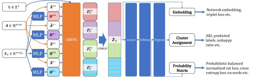
Figure 1: SSSNET overview: starting from feature matrix $\mathbf{X}_{\mathcal{V}}$ and adjacency matrix $\mathbf{A}$, we first compute the row-normalized adjacency matrices $\overline{\mathbf{A}}^{s+},\overline{\mathbf{A}}^{s-},\overline{\mathbf{A}}^{t+}$, $\overline{\mathbf{A}}^{t-}.$ We then apply four separate MLPs on $\mathbf{X}_{\mathcal{V}},$ to obtain hidden representations $\mathbf{H}^{s+},\mathbf{H}^{s-},\mathbf{H}^{t+},$ $\mathbf{H}^{t-},$ respectively. Next, we compute their decoupled embeddings via Eq. (3.1) and its equivalent for negative/target embeddings. The concatenated decoupled embeddings are the final embeddings. We add another linear layer followed by a unit softmax function to obtain the probability matrix $\mathbf{P}$. Applying argmax to each row of $\mathbf{P}$ yields cluster assignments for all nodes.

From a method’s viewpoint, the neutral stance is reflected in the feature aggregation in SIMPA, which provides the basis of the network embedding. Network clustering is then carried out using the node embedding as input and a loss function for training; see Figure 1 for an overview. To train SSSNET, the loss function consists of a self-supervised novel probabilistic balanced normalized cut loss acting on all training nodes, and a supervised loss which acts on seed nodes, if available. Experimental results at different scales demonstrate that our method achieves state-of-the-art performance on synthetic data, for a wide range of network densities, while complementing other methods through the possibility of incorporating exogenous information. Tested on real-world data for which ground truth is available, our method outperforms its competitors in terms of the Adjusted Rand Index [28].

Main contributions. Our main contributions are as follows: $\bullet$ (1) An efficient end-to-end GNN for semi-supervised signed node clustering, based on a new variant of social balance theory. To the best of our knowledge, this is the first GNN-based method deriving node embeddings for clustering signed networks, potentially with attributes. The advantage of the ability to handle features is that we can incorporate eigen-features of other methods (such as eigenvectors of the signed Laplacian), thus borrowing strength from existing methods. $\bullet$ (2) A Signed Mixed-Path Aggregation (SIMPA) framework based on our new take on social balance theory. $\bullet$ (3) A probabilistic version of balanced normalized cut to serve as a self-supervised loss function for signed clustering. $\bullet$ (4) We achieve state-of-the-art performance on various signed clustering tasks, including a challenging version of a classification task, for which we customize and adapt a general definition of polarized signed stochastic block models (Pol-SSBM), to include an ambient cluster and multiple polarized SSBM communities, not necessarily of equal size, but of equal density. Code and preprocessed data are available at https://github.com/SherylHYX/SSSNET_Signed_Clustering. An alternative implementation is available in the open-source library PyTorch Geometric Signed Directed [24].

2 Related Work

2.1 Network Embedding and Clustering

We introduce a semi-supervised method for node embeddings, which uses the idea of an aggregator and relies on powers of adjacency matrices for such aggregators. The use of an aggregation function is motivated by [21]. The use of powers of adjacency matrices for neighborhood information aggregation was sparked by a mechanism for node feature aggregation, proposed in [48], with a data-driven similarity metric during training.

Non-GNN methods have been employed for signed clustering. [32] uses the signed Laplacian matrix and its normalized versions for signed clustering. [38] clusters signed networks using the geometric mean of Laplacians.In [12], nodes are clustered based on optimizing the Balanced Normalized Cut and the Balanced Ratio Cut. [58] develops two normalized signed Laplacians based on the so-called SNScut and BNScut. [14] relies on a generalized eigenproblem and achieves state-of-the-art performance on signed clustering. To conduct semi-supervised structural learning on signed networks, [36] uses variational Bayesian inference and [16] devises an MBO scheme. [6] tackles network sparsity. However, these prior works do not take node attributes into account. [51] exploits the network structure and node attributes simultaneously, but does not utilize known labels. [55] views relationship formation between users as the comprehensive effects of latent factors and trust transfer patterns, via social balance theory.

GNNs have also been used for signed network embedding tasks, but not for signed clustering. SGCN [17] employs social balance theory to aggregate and propagate the information across layers. Considering joint interactions between positive and negative edges is another main inspiration for our method. Many other GNNs [27, 26, 35, 11, 33, 57] are also based on social balance theory, usually applied to data with strong positive class imbalance. Numerous other signed network embedding methods [9, 10, 52, 29, 55] also do not explore the node clustering problem. Hence we do not employ these methods for comparison.

2.2 Polarization

Opinion formation in a social network can be driven by a few small groups which have a polarized opinion, in a social network in which many agents do not (yet) have a strongly formed opinion. These small clusters could strongly influence the public discourse and even threaten the integrity of democratic processes. Detecting such small clusters of polarized agents in a network of ambient nodes is hence of interest [54]. For a network with node set $\mathcal{V}$, [54] introduces the notion of a polarized community structure $(\mathcal{C}_{1},\mathcal{C}_{2})$ within the wider network, as two disjoint sets of nodes $\mathcal{C}_{1},\mathcal{C}_{2}\subseteq\mathcal{V},$ such that $\bullet$(1) there are relatively few (resp. many) negative (resp. positive) edges within $\mathcal{C}_{1}$ and within $\mathcal{C}_{2};$ $\bullet$(2) there are relatively few (resp. many) positive (resp. negative) edges across $\mathcal{C}_{1}$ and $\mathcal{C}_{2};$ $\bullet$(3) there are relatively few edges (of either sign) from $\mathcal{C}_{1}$ and $\mathcal{C}_{2}$ to the rest of the graph. By allowing a subset of nodes to be neutral with respect to the polarized structure, [49] derives a formulation in which each cluster inside a polarized community is naturally characterized by the solution to the maximum discrete Rayleigh’s quotient (MAX-DRQ) problem. However, this model cannot incorporate node attributes. Extending the approach in [7] and [14], here, a community structure $(\mathcal{C}_{1},\mathcal{C}_{2})$ is said to be polarized if (1) and (2) hold, while (3) is not required to hold. Moreover, our model includes different parameters for the noise and edge probability.

3 The SSSNET Method

3.1 Problem Definition

Denote a signed network with node attributes as $\mathcal{G}=(\mathcal{V},\mathcal{E},w,\mathbf{X}_{\mathcal{V}}),$ where $\mathcal{V}$ is the set of nodes, $\mathcal{E}$ is the set of (directed) edges or links, and $w\in(-\infty,\infty)^{|\mathcal{E}|}$ is the set of weights of the edges. Here $\mathcal{G}$ could have self-loops but not multiple edges. The total number of nodes is $n=|\mathcal{V}|,$ and $\mathbf{X}_{\mathcal{V}}\in\mathbb{R}^{n\times d_{\text{in}}}$ is a matrix whose rows are node attributes. These attributes could be generated from the adjacency matrix $\mathbf{A}$ with entries $\mathbf{A}_{ij}=w_{ij}$, the edge weight, if there is an edge between nodes $v_{i}$ and $v_{j}$; otherwise $\mathbf{A}_{ij}=0$. We decompose $\mathbf{A}$ into its positive and negative part $\mathbf{A}^{+}$ and $\mathbf{A}^{-},$ where $\mathbf{A}_{ij}^{+}=\max(\mathbf{A}_{ij},0)$ and $\mathbf{A}_{ij}^{-}=-\min(\mathbf{A}_{ij},0).$ A clustering into $K$ clusters is a partition of the node set into disjoint sets $\mathcal{V}=\mathcal{C}_{0}\cup\mathcal{C}_{1}\cup\cdots\cup\mathcal{C}_{K-1}.$ Intuitively, nodes within a cluster should be similar to each other, while nodes across clusters should be dissimilar. In a semi-supervised setting, for each of the $K$ clusters, a fraction of training nodes are selected as seed nodes, for which the cluster membership labels are known before training. The set of seed nodes is denoted as $\mathcal{V}^{\text{seed}}\subseteq\mathcal{V}^{\text{train}}\subset\mathcal{V},$ where $\mathcal{V}^{\text{train}}$ is the set of all training nodes. For this task, the goal is to use the embedding for assigning each node $v\in\mathcal{V}$ to a cluster containing known seed nodes. When no seeds are given, we are in a self-supervised setting, where only the number of clusters, $K,$ is given.

3.2 Path-Based Node Relationship

Methods based on social balance theory assume that, given a negative relationship between $v_{1},v_{2}$ and a negative relationship between $v_{2},v_{3}$, the nodes $v_{1}$ and $v_{3}$ should be positively related. This assumption may be sensible for social networks, but in other networks such as correlation networks [1, 4], it is not obvious why it should hold. Indeed, the column $|\Delta^{\text{u}}|$ in Table 1 counts the number of triangles with an odd number of negative edges in eight real-world data sets and one synthetic model. We observe that $|\Delta^{\text{u}}|$ is never zero, and that in some cases, the percentage of unbalanced triangles (the last column) is quite large, such as in Sampson’s network of novices and the simulated SSBM($n=5000,K=5,p=0.1,\rho=1.5$) (“Syn” in Table 1, SSBM is defined in Section 4.1.1). The relative high proportion of unbalanced triangles sparks our novel approach. SSSNET holds a neutral attitude towards the relationship between $v_{1}$ and $v_{3}.$ In contrast to social balance theory, our definition of “friends” and “enemies” is based on the set of paths within a given length between any two nodes. For a target node $v_{j}$ to be an $h$-hop “friend” neighbor of source node $v_{i}$ along a given path from $v_{i}$ to $v_{j}$ of length $h$, all edges on this path need to be positive. For a target node $v_{j}$ to be an ${h}$-hop “enemy” neighbor of source node $v_{i}$ along a given path from $v_{i}$ to $v_{j}$ of length $h$, exactly one edge on this path has to be negative. Otherwise, $v_{i}$ and $v_{j}$ are neutral to each other on this path. For directed networks, only directed paths are taken into account, and the friendship relationship is no longer symmetric.

Figure 2 illustrates five different paths of length four, connecting the source and the target nodes. We can also obtain the relationship of a source node to a target node within a path by reversing the arrows in Figure 2. Note that it is possible for a node to be both a “friend” and an “enemy” to a source node simultaneously, as there might be multiple paths between them, with different resulting relationships. Our model aggregates these relationships by assigning different weights to different paths connecting two nodes. For example, the source node and target node may have all five paths shown in Figure 2 connecting them. Since the last two paths are neutral paths and do not cast a vote on their relationship, we only take the top three paths into account. We refer to the long-range neighbors whose information would be considered by a node as the contributing neighbors with respect to the node of interest.

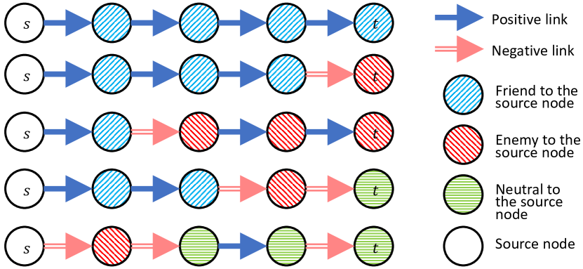
Figure 2: Example: five paths between the source (s) and target (t) nodes, and resulting relationships. While we assume a neutral relationship on the last two paths, social balance theory claims them as ”friend” and ”enemy”, respectively.

3.3 Signed Mixed-Path Aggregation (SIMPA)

SIMPA aggregates neighbor information from contributing neighbors within $h$ hops, by a weighted average of the embeddings of the up-to-$h$-hop contributing neighbors of a node, with the weights constructed in analogy to a random walk on the set of nodes.

3.3.1 SIMPA Matrices

First, we row-normalize $\mathbf{A}^{+}$ and $\mathbf{A}^{-}$, to obtain matrices $\mathbf{\overline{A}}^{s+}$ and $\mathbf{\overline{A}}^{s-}$, respectively. Inspired by the regularization discussed in [31], we add a weighted self-loop to each node and carry out the normalization by setting $\mathbf{\overline{A}^{s+}=(\tilde{D}}^{s+})^{-1}\mathbf{\tilde{A}}^{s+},$ where $\mathbf{\tilde{A}}^{s+}=\mathbf{A}^{+}+\tau^{+}\mathbf{I}$ and the diagonal matrix $\mathbf{\tilde{D}}^{s+}(i,i)=\sum_{j}\mathbf{\tilde{A}}^{s+}(i,j),$ for some $\tau^{+}\geq 0$; similarly, we row-normalize $\mathbf{A}^{s-}$ to obtain $\mathbf{\overline{A}}^{s-}$ based on $\tau^{-}.$ Next, we explore multi-hop neighbors by taking powers or mixed powers of $\mathbf{\overline{A}}^{s+}$ and $\mathbf{\overline{A}}^{s-}.$ The $h$-hop “friend” neighborhood can be computed directly from $(\overline{\mathbf{A}}^{s+})^{h}$, the $h^{th}$ power of $\overline{\mathbf{A}}^{s+}$. Similarly, the $h$-hop “enemy” neighborhood is computed directly from the mixed powers of $h-1$ terms of $\overline{\mathbf{A}}^{s+},$ and exactly one term of $\mathbf{\overline{A}}^{s-}.$ We denote the set of up-to-$h$-hop “friend” neighborhood matrices as $\mathcal{A}^{s+,h}=\{(\mathbf{\overline{A}}^{s+})^{h_{1}}:h_{1}\in\{0,\cdots,h\}\},$ where $(\mathbf{\overline{A}}^{s+})^{0}=\mathbf{I},$ the identity matrix, and the set of up-to-$h$-hop “enemy” neighborhood matrices as

$$\vspace{-1mm}\mathcal{A}^{s-,h}=\left\{(\mathbf{\overline{A}}^{s+})^{h_{1}}\cdot\mathbf{\overline{A}}^{s-}\cdot(\mathbf{\overline{A}}^{s+})^{h_{2}}:h_{1},h_{2}\in H\right\}\vspace{-1mm}$$

with $H=\{(h_{1},h_{2}):h_{1},h_{2}\in\{0,\ldots,h-1\},h_{1}+h_{2}\leq h-1\}$. With added self-loops, any $h$-hop neighbor defined by our matrices aggregates beliefs from nearby neighbors. Since a node is not an enemy to itself, we set $\tau^{-}=0.$ We use $\tau^{+}=\tau=0.5$ in our experiments.

When the signed network is directed, we additionally carry out $\ell_{1}$ row normalization and calculate mixed powers for $(\mathbf{A}^{+})^{T}$ and $(\mathbf{A}^{-})^{T}.$ We denote the row-normalized adjacency matrices for target positive and negative as $\overline{\mathbf{A}}^{t+}$ and $\overline{\mathbf{A}}^{t-},$ respectively. Likewise, we denote the set of up-to-$h$-hop target “friend” (resp. “enemy”) neighborhood matrices as $\mathcal{A}^{t+,h}$ (resp. $\mathcal{A}^{t-,h}$).

3.3.2 Feature Aggregation Based on SIMPA

Next, we define four feature-mapping functions for source positive, source negative, target positive and target negative embeddings, respectively. A source positive embedding of a node is the weighted combination of its contributing neighbors’ hidden representations, for neighbors up to $h$ hops away. The source positive hidden representation is denoted as $\mathbf{H}_{\mathcal{V}}^{s+}\in\mathbb{R}^{n\times d}$. Assume that each node in $\mathcal{V}$ has a vector of features and summarize these features in the input feature matrix $\mathbf{X_{\mathcal{V}}}$. The source positive embedding $\mathbf{Z}^{s+}_{\mathcal{V}}$ is given by

(3.1) $$\vspace{-2mm}\mathbf{Z}^{s+}_{\mathcal{V}}=\sum_{\mathbf{M}\in\mathcal{A}^{s+,h}}\omega_{{\mathbf{M}}}^{s+}\cdot{\mathbf{M}}\cdot\mathbf{H}_{\mathcal{V}}^{s+}\in\mathbb{R}^{n\times d},$$

where for each $\mathbf{M},$ $\omega_{\mathbf{M}}^{s+}$ is a learnable scalar, and $d$ is the embedding dimension. In our experiments, we use $\mathbf{H}_{\mathcal{V}}^{s+}=\textbf{MLP}^{(s+,l)}(\mathbf{X}_{\mathcal{V}}).$ The hyperparameter $l$ controls the number of layers in the multilayer perceptron (MLP) with ReLU activation; we fix $l=2$ throughout. Each layer of the MLP has the same number $d$ of hidden units.

The embeddings $\mathbf{Z}^{s-}_{\mathcal{V}}$, $\mathbf{Z}^{t+}_{\mathcal{V}}$ and $\mathbf{Z}^{t-}_{\mathcal{V}}$ for source negative embedding, target positive embedding and target negative embedding, respectively, are defined similarly. Different parameters for the MLPs for different embeddings are possible. We concatenate the embeddings to obtain the final node embedding as a $n\times(4d)$ matrix $\mathbf{Z}_{\mathcal{V}}=\operatorname{CONCAT}\left(\mathbf{Z}_{\mathcal{V}}^{s+},\mathbf{Z}_{\mathcal{V}}^{s-},\mathbf{Z}_{\mathcal{V}}^{t+},\mathbf{Z}_{\mathcal{V}}^{t-}\right).$ The embedding vector $\mathbf{z}_{i}$ for a node $v_{i},$ is the $i^{\text{th}}$ row of $\mathbf{Z}_{\mathcal{V}}$, namely $\mathbf{z}_{i}:=(\mathbf{Z}_{\mathcal{V}})_{(i,:)}\in\mathbb{R}^{4d}.$ Next we apply a linear layer to $\mathbf{Z}_{\mathcal{V}}$ so that the resulting matrix has the same number of columns as the number $K$ of clusters. We apply the unit softmax function to map each row to a probability vector $\mathbf{p}_{i}\in\mathbb{R}^{K}$ of length equal to the number of clusters, with entries denoting the probabilities of each node to belong to each cluster. The resulting probability matrix is denoted as $\mathbf{P}\in\mathbb{R}^{n\times K}.$ If the input network is undirected, it suffices to find $\mathcal{A}^{s+,h}$ and $\mathcal{A}^{s-,h},$ and we obtain the final embedding as $\mathbf{Z}_{\mathcal{V}}=\operatorname{CONCAT}\left(\mathbf{Z}_{\mathcal{V}}^{s+},\mathbf{Z}_{\mathcal{V}}^{s-}\right)\in\mathbb{R}^{n\times(2d)}.$

3.4 Loss, Overview & Complexity Analysis

Node clustering is optimized to minimize a loss function which pushes embeddings of nodes within the same cluster close to each other, while driving apart embeddings of nodes from different clusters. We first introduce a novel self-supervised loss function for node clustering, then discuss supervised loss functions when labels are available for some seed nodes.

3.4.1 Probabilistic Balanced Normalized Cut Loss

For a clustering $(\mathcal{C}_{0},\ldots\mathcal{C}_{K-1})$, let $\{\mathbf{x}_{0},\cdots,\mathbf{x}_{K-1}\}$ denote the cluster indicator vectors so that $\mathbf{x}_{k}(i)=1$ if node $i$ is in cluster $C_{k}$, and 0 otherwise. Let $\mathbf{L}^{+}=\mathbf{D}^{+}-\mathbf{A}^{+}$ denote the unnormalized graph Laplacian for the positive part of $\mathbf{A},$ where $\mathbf{D}^{+}$ is a diagonal matrix whose diagonal entries are row-sums of $\mathbf{A}^{+}.$ Then $\mathbf{x}_{k}^{T}\mathbf{L}^{+}\mathbf{x}_{k}$ measures the total weight of positive edges linking cluster ${\mathcal{C}_{k}}$ to other clusters. Further, $\mathbf{x}_{k}^{T}\mathbf{A}^{-}\mathbf{x}_{k}$ measures the total weight of negative edges within cluster ${\mathcal{C}_{k}}$. Since $\mathbf{D}^{+}-\mathbf{A}=\mathbf{D}^{+}-\mathbf{A}^{+}+\mathbf{A}^{-}$, then $\mathbf{x}_{k}^{T}(\mathbf{L}^{+}+\mathbf{A}^{-})\mathbf{x}_{k}=\mathbf{x}_{k}^{T}(\mathbf{D}^{+}-\mathbf{A})\mathbf{x}_{k}$ measures the total weight of the unhappy edges with respect to cluster ${\mathcal{C}_{k}}$; “unhappy edges” violate their expected signs (positive edges across clusters or negative edges within clusters). The loss function in this paper is related to the (non-differentiable) Balanced Normalized Cut (BNC) [12]. In analogy, we introduce the differentiable Probabilistic Balanced Normalized Cut (PBNC) loss

(3.2) $$\mathcal{L}_{\text{PBNC}}=\sum_{k=1}^{K}\frac{(\mathbf{P}_{(:,k)})^{T}(\mathbf{D}^{+}-\mathbf{A})\mathbf{P}_{(:,k)}}{(\mathbf{P}_{(:,k)})^{T}\mathbf{\overline{D}}\mathbf{P}_{(:,k)}},\vspace{-2mm}$$

where $\mathbf{P}_{(:,k)}$ denotes the $k^{th}$ column of the probability matrix $\mathbf{P}$ and $\overline{\mathbf{D}}_{ii}=\sum_{j=1}^{n}|A_{ij}|$. As column $k$ of $\mathbf{P}$ is a relaxed version of $\mathbf{x}_{k}$, the numerator in Eq. (3.2) is a probabilistic count of the number of unhappy edges.

3.4.2 Supervised Loss

When some seed nodes have known labels, a supervised loss can be added to the loss function. For nodes in $\mathcal{V}^{\text{seed}},$ we use as a supervised loss function similar to that in [48], the sum of a cross entropy loss $\mathcal{L}_{\text{CE}}$ and a triplet loss. The triplet loss is

(3.3) $$\mathcal{L}_{\text{triplet}}=\frac{1}{|\mathcal{T}|}\sum_{(v_{i},v_{j},v_{k})\in\mathcal{T}}ReLU(\operatorname{CS}(\mathbf{z}_{i},\mathbf{z}_{j})-\operatorname{CS}(\mathbf{z}_{i},\mathbf{z}_{k})+\alpha),\vspace{-2mm}$$

where $\mathcal{T}\subseteq\mathcal{V}^{\text{seed}}\times\mathcal{V}^{\text{seed}}\times\mathcal{V}^{\text{seed}}$ is a set of node triplets: $v_{i}$ is an anchor seed node, and $v_{j}$ is a seed node from the same cluster as the anchor, while $v_{k}$ is from a different cluster. Here, $\operatorname{CS}(\mathbf{z}_{i},\mathbf{z}_{j})$ is the cosine similarity of the embeddings of nodes $v_{i}$ and $v_{j}$, chosen so as to avoid sensitivity to the magnitude of the embeddings. $\alpha\geq 0$ is the contrastive margin as in [48]. $\mathcal{L}_{\text{CE}}+\gamma_{t}\mathcal{L}_{\text{triplet}}$ forms the supervised part of the loss function for SSSNET, for a suitable parameter $\gamma_{t}>0.$

3.4.3 Overall Objective Function and Framework Overview

By combining $\mathcal{L}_{\text{CE}}$, Eq. (3.2), and Eq. (3.3), the objective function minimizes

(3.4) $$\vspace{-2mm}\mathcal{L}=\mathcal{L}_{\text{PBNC}}+\gamma_{s}(\mathcal{L}_{\text{CE}}+\gamma_{t}\mathcal{L}_{\text{triplet}}),$$

where $\gamma_{s},\gamma_{t}>0$ are weights for the supervised part of the loss and triplet loss, respectively. The final embedding can then be used, for example, for node clustering. A linear layer coupled with a unit softmax function turns the embedding into a probability matrix. A node is assigned to the cluster for which its membership probability is highest. Figure 1 gives an overview.

3.4.4 Complexity Analysis

The matrix operations in Eq. (3.1) appear to be computationally expensive and space unfriendly. However, SSSNET resolves these concerns via a sparsity-aware implementation, detailed in Algorithm 1 in SI C.1, without explicitly calculating the sets of powers, maintaining sparsity throughout. Therefore, for input feature dimension $d_{\text{in}}$ and hidden dimension $d$, if $d^{\prime}=\max(d_{\text{in}},d)\ll n,$ time and space complexity of SIMPA, and implicitly SSSNET, is $\mathcal{O}(|\mathcal{E}|d^{\prime}h^{2}+4nd^{\prime}K)$ and $\mathcal{O}(4|\mathcal{E}|+10nd^{\prime}+nK),$ respectively [19]. For large networks, SIMPA is amenable to a more scalable version following [18].

4 Experiments

This section describes the synthetic and real-world data sets used in this study, and illustrates the efficacy of our method. When ground truth is available, performance is measured by the Adjusted Rand Index (ARI) [28]. When no labels are provided, we measure performance by the ratio of number of “unhappy edges” to that of all edges. Our self-supervised loss function is applied to the subgraph induced by all training nodes. We do not report Normalized Mutual Information (NMI) [42] performance in Figure 5 (but reported in SI A.1 ) as it has some shortcomings [2], and results from the ARI and NMI from our synthetic experiments indeed yield almost the same ranking for the methods, with average Kendall tau 0.808 and standard deviation 0.233.

4.1 Data

4.1.1 Synthetic Data: Signed Stochastic Block Models (SSBM)

A Signed Stochastic Block Model (SSBM) for a network on $n$ nodes with $K$ blocks (clusters), is constructed similar to [14] but with a more general cluster size definition.

In our experiments, we choose the number of clusters, the (approximate) ratio, $\rho$, between the largest and the smallest cluster size, sign flip probability, $\eta$, and the number, $n$, of nodes. To tackle the hardest clustering task, all pairs of nodes within a cluster and those between clusters have the same edge probability, with more details in SI B.1. Our SSBM model can be represented by SSBM($n,K,p,\rho,\eta$).

4.1.2 Synthetic Data: Polarized SSBMs

In a polarized SSBM model, SSBMs are planted in an ambient network; each block of each SSBM is a cluster, and the nodes not assigned to any SSBM form an ambient cluster. The polarized SSBM model that creates communities of SSBMs, is generated as follows: $\bullet$(1) Generate an Erdős-Rényi graph with $n$ nodes and edge probability $p,$ whose sign is set to $\pm 1$ with equal probability 0.5. $\bullet$(2) Fix $n_{c}$ as the number of SSBM communities, and calculate community sizes $N_{1}\leq N_{2}\leq\cdots\leq N_{r},$ for each of the $r$ communities as in Section 4.1.1, such that the ratio of the largest block size to the smallest block size is approximately $\rho$, and the total number of nodes in these SSBMs is $N\times n_{c}.$ $\bullet$(3) Generate $r$ SSBM models, each with $K_{i}=2,i=1,\ldots,r$ blocks, number of nodes according to its community size, with the same edge probability $p$, size ratio $\rho$, and flip probability $\eta$. $\bullet$(4) Place the SSBM models on disjoint subsets of the whole network; the remaining nodes not part of any SSBM are dubbed as ambient nodes.

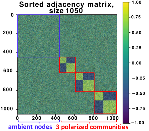
(a) Sorted adjacency matrix.

(b) Polarized community #1.

Figure 3: A polarized SSBM model with 1050 nodes, $r=3$ polarized communities of sizes 161, 197, and 242; $\rho=1.5,$ default SSBM community size $N=200,p=0.5,\eta=0.05,$ and each SSBM has $K_{1}=K_{2}=K_{3}=2$ blocks, rendering $K=7$.

Therefore, while the total number of clusters in an SSBM equals the number of blocks, the total number of clusters within a polarized SSBM model equals $K=1+\sum_{i=1}^{r}K_{i}=1+2r.$ In our experiments, we also assume the existence of an ambient cluster. The resulting polarized SSBM model is denoted as Pol-SSBM ($n,r,p,\rho,\eta,N$). The setting in [7] can be construed as a special case of our model, see SI B.2.

Figure 3 gives a visualization of a polarized SSBM model with 1050 nodes, $p=0.5,\eta=0.05,N=200,$ with 3 SSBMs of $K=2$ blocks each, $\rho=1.5.$ The sorted adjacency matrix has its rows and columns sorted by cluster membership, starting with the ambient cluster. With $\rho=1.5,$ the largest SSBM community has size 242, while the smallest has size 161, as $\frac{242}{161}\approx 1.5=\rho.$ For $n=1050,$ the default size of a SSBM community is $N=200.$ For $n=5000$ (resp, $n=10000$) we consider $N=500$ (resp. $N=2000$).

4.1.3 Real-World Data

We perform experiments on six real-world signed network data sets (Sampson [43], Rainfall [5], Fin-YNet, S&P 1500 [56], PPI [50], and Wiki-Rfa [53]), summarized in Table 1. Sampson, as the only data set with given node attributes (1D “Cloisterville” binary attribute), cover four social relationships, which are combined into a network; Rainfall contains Australian rainfalls pairwise correlations; Fin-YNet consists of 21 yearly financial correlation networks and its results are averaged; S&P1500 is a correlation network of stocks during 2003-2005; PPI is a signed protein-protein interaction network; Wiki-Rfa describes voting information for electing Wikipedia managers.

We use labels given by each data set for Sampson (5 clusters), and sector memberships for S&P 1500 and Fin-YNet (10 clusters). For Rainfall, with 6 clusters, we use labels from SPONGE as proxy for ground truth to carry out semi-supervised learning. For other data sets with no “ground-truth” labels available, we train SSSNET in a self-supervised manner, using all nodes to train. By exploring performance on SPONGE, we set the number of clusters for Wiki-Rfa as three, and similarly ten for PPI. Additional details concerning the data and preprocessing steps are available in SI B.

Table 1: Summary statistics for the real-world networks and one synthetic model. Here $n$ is the number of nodes, $|\mathcal{E}^{+}|$ and $|\mathcal{E}^{-}|$ denote the number of positive and negative edges, respectively. $|\Delta^{\text{u}}|$ counts the number of unbalanced triangles (with an odd number of negative edges). The violation ratio $\frac{|\Delta^{\text{u}}|}{|\Delta|}$ (%) is the percentage of unbalanced triangles in all triangles, i.e., 1 minus the Social Balance Factor from [39].

Data set	$n$	$|\mathcal{E}^{+}|$	$|\mathcal{E}^{-}|$	$|\Delta^{\text{u}}|$	$\frac{|\Delta^{\text{u}}|}{|\Delta|}$ (%)
Sampson	25	129	126	192	37.16
Rainfall	306	64,408	29,228	1,350,756	28.29
Fin-YNet	451	14,853	5,431	408,594	26.97
S&P 1500	1,193	1,069,319	353,930	199,839	28.15
PPI	3,058	7,996	3,864	94	2.45
Syn	5,000	510,586	198,6224	9,798,914	47.20
Wiki-Rfa	7,634	136,961	38,826	79,911,143	28.23

4.2 Experimental Results

In our experiments, we compare SSSNET against nine state-of-the-art spectral clustering methods in signed networks mentioned in Sec. 2. These methods are based on: (1) the symmetric adjacency matrix $\mathbf{A}^{*}=\frac{1}{2}(\mathbf{A}+(\mathbf{A})^{T}),$ (2) the simple normalized signed Laplacian $\mathbf{\bar{L}}_{sns}=\bar{\mathbf{D}}^{-1}(\mathbf{D}^{+}-\mathbf{D}^{-}\mathbf{A}^{*})$ and (3) the balanced normalized signed Laplacian $\mathbf{\bar{L}}_{bns}=\bar{\mathbf{D}}^{-1}(\mathbf{D}^{+}-\mathbf{A}^{*})$ [58], (4) the Signed Laplacian matrix $\mathbf{\bar{L}}$ of $\mathbf{A}^{*},$ (5) its symmetrically normalized version $\mathbf{L}_{\text{sym}}$ [32], and the two methods from [12] to optimize the (6) Balanced Normalized Cut and the (7) Balanced Ratio Cut, (8) SPONGE and (9) SPONGE_sym introduced in [14], where the diagonal matrices $\mathbf{\bar{D}},\mathbf{D}^{+}$ and $\mathbf{D}^{-}$ have entries as row-sums of $(\mathbf{A}^{*})^{+}+(\mathbf{A}^{*})^{-},(\mathbf{A}^{*})^{+}$ and $(\mathbf{A}^{*})^{-}$, respectively. In our experiments, the abbreviated names of these methods are A, sns, dns, L, L_sym, BNC, BRC, SPONGE, and SPONGE_sym, respectively. The implementation details are in SI C.

Hyperparameter selection is done via greedy search.

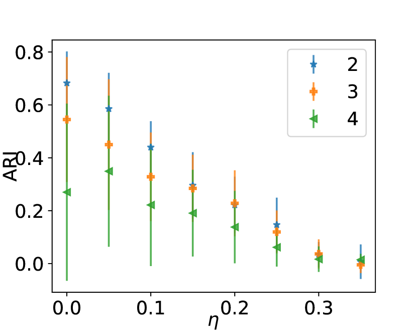
(a) Vary hop $h$ for SIMPA.

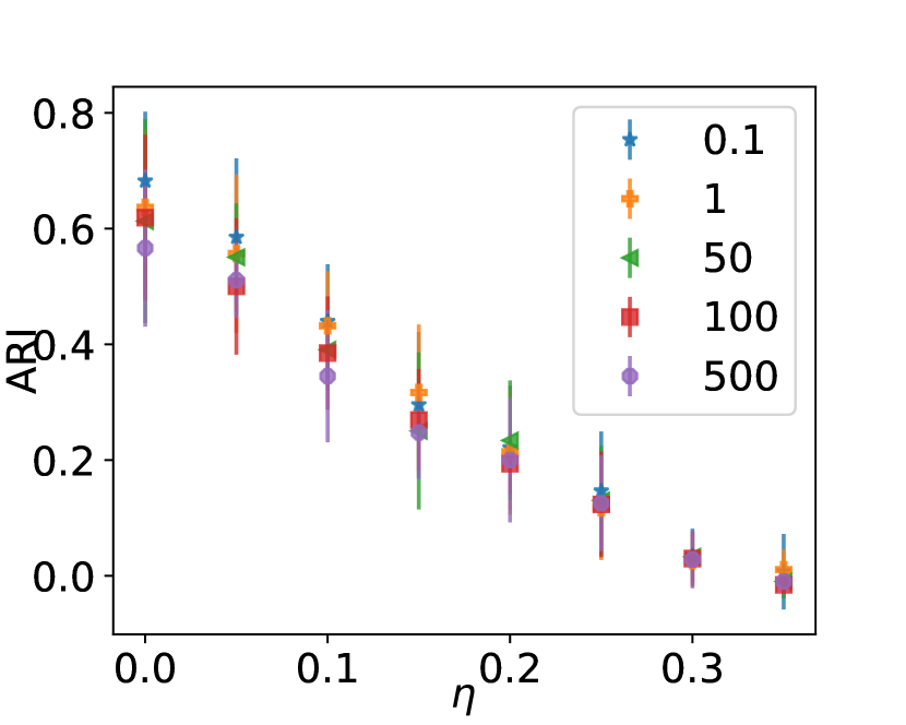
(b) Vary $\gamma_{t}$ in Eq. (3.4).

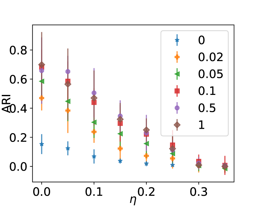
(c) Vary seed ratio.

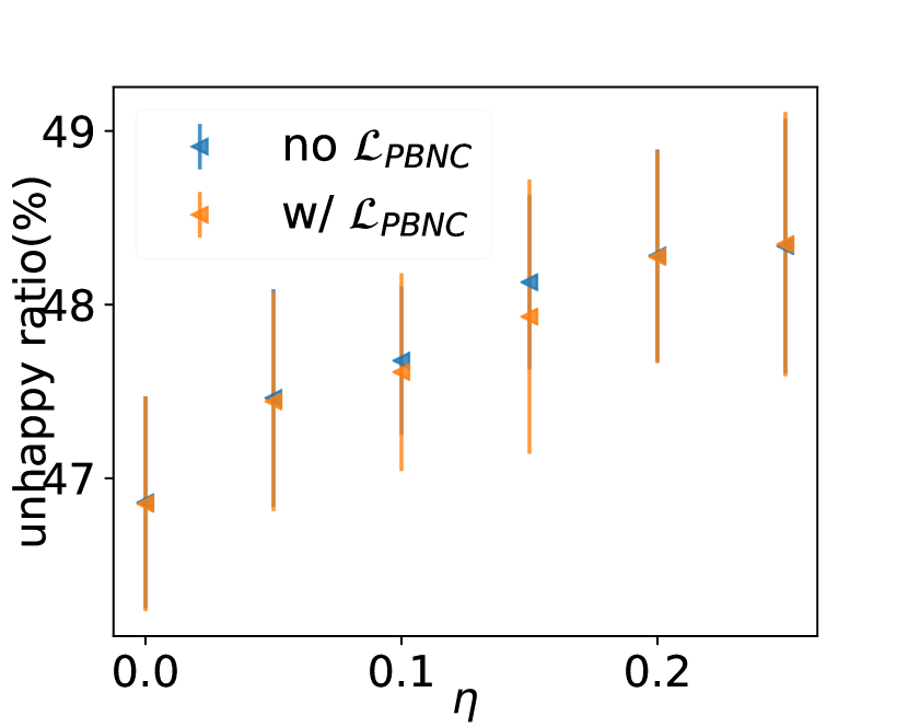
(d) With/without the self-supervised part $\mathcal{L}_{\text{PBNC}}$ in Eq. (3.4).

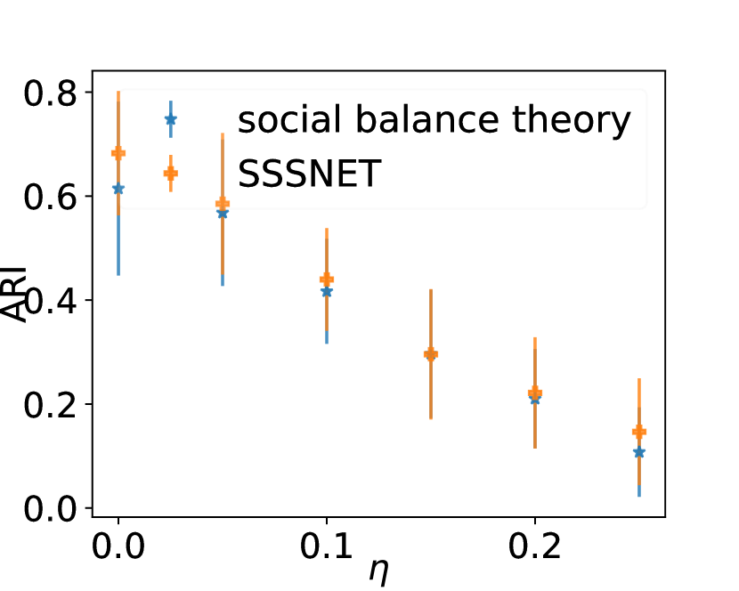
(e) Social balance theory vs SSSNET (as we vary $\eta$).

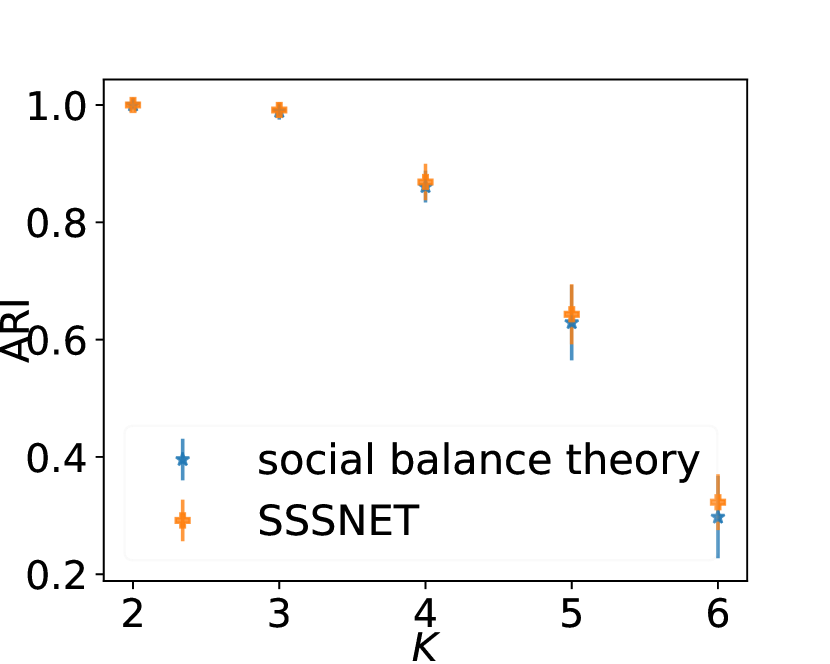
(f) Social balance theory vs SSSNET (as we vary $K$).

Figure 4: Hyperparameter analysis (a,b) and ablation study (c-f). Figures (a-e) pertain to Pol-SSBM($n=1050,r=2,p=0.1,\rho=1.5$), while Figure (f) is for an SSBM($n=1000,\eta=0,p=0.01,\rho=1.5$) model with changing $K.$ Figure (d) compares the “unhappy ratio” while the others compare the test ARI.

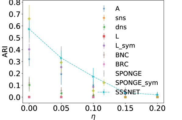
(a) SSBM($n=1000,$
$K=5,p=0.01,\rho=1.5$)

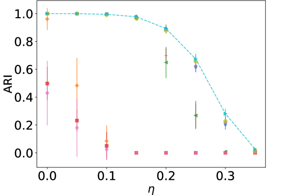
(b) SSBM($n=5000,$
$K=5,p=0.01,\rho=1.5$)

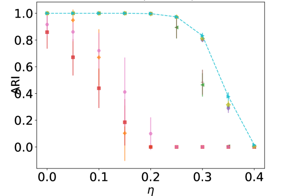
(c) SSBM($n=10000,$
$K=5,p=0.01,\rho=1.5)$

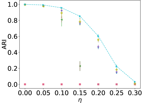
(d) SSBM($n=30000,$
$K=5,p=0.001,\rho=1.5$)

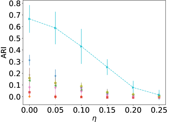
(e) Pol-SSBM($n=1050,$
$r=2,p=0.1,\rho=1$)

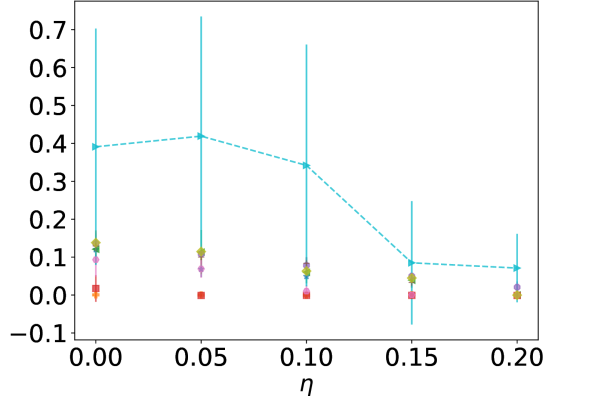
(f) Pol-SSBM($n=5000,$
$r=3,p=0.1,\rho=1.5$)

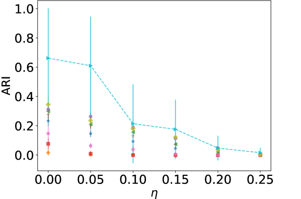
(g) Pol-SSBM($n=5000,$
$r=5,p=0.1,\rho=1.5$)

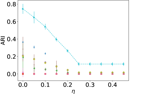
(h) Pol-SSBM($n=10000,$
$r=2,p=0.01,\rho=1.5$)

Figure 5: Node clustering test ARI comparison on synthetic data. Dashed lines highlight SSSNET’s performance. Error bars indicate one standard error.

Figure 4 (a-b) compare the performance of SSSNET on a Pol-SSBM($n=1050,r=2,p=0.1,\rho=1.5$) model under different settings. We conclude from (a) that as we increase the number of hops to consider, performance drops, which might be explained by too much noise introduced. From (b), we find that the best $\gamma_{t}$ in our candidates is 0.1. See also SI C.4. Our default setting is $h=2,d=32,\tau=0.5,\gamma_{s}=50,\gamma_{t}=0.1,\alpha=0.$

Unless specified otherwise, we use 10% of all nodes from each cluster as test nodes, 10% as validation nodes to select the model, and the remaining 80% as training nodes, 10% of which as seed nodes. We train SSSNET for at most 300 epochs with a 100-epoch early-stopping scheme. As Sampson is small, 50% nodes are training nodes, 50% of which are seed nodes, and no validation nodes; we train 80 epochs and test on the remaining 50% nodes. For S&P 1500, Fin-YNet and Rainfall, we use 90% nodes for training, 10% of which as seed nodes, and no validation nodes for 300 epochs. If node attributes are missing, SSSNET stacks the eigenvectors corresponding to the largest $K$ eigenvalues of the symmetrized adjacency matrix $\frac{1}{2}(\mathbf{A}+\mathbf{A}^{T})$ as $\mathbf{X}_{\mathcal{V}}$ for synthetic data, and the eigenvectors corresponding to the smallest $K$ eigenvalues of the symmetrically normalized Signed Laplacian [25] of $\frac{1}{2}(\mathbf{A}+\mathbf{A}^{T})$ for real-world data. Numerical results are averaged over 10 runs; error bars indicate one standard error.

4.2.1 Node Clustering Results on Synthetic Data

Figure 5 compares the numerical performance of SSSNET with other methods on synthetic data. We remark that SSSNET gives state-of-the-art test ARIs on a wide range of network densities and noise levels, on various network scales, especially for polarized SSBMs. SI A.1 provides more results with different measures.

4.2.2 Node Clustering Results on Real-World Data

Table 2: Clustering performance on real-world data sets; best is in bold red, and $2^{\text{nd}}$ in underline blue. The first 3 rows are test ARIs, the $4^{\text{th}}$ “ARI distance to best”, the rest are unhappy ratios (%).

Data set	A	sns	dns	L	L_sym	BNC	BRC	SPONGE	SPONGE_sym	SSSNET
Sampson	0.32$\pm$0.10	0.15$\pm$0.09	0.33$\pm$0.10	0.16$\pm$0.05	0.35$\pm$0.09	0.32$\pm$0.12	0.21$\pm$0.11	0.36$\pm$0.11	0.34$\pm$0.11	0.55$\pm$0.07
Rainfall	0.61$\pm$0.08	0.28$\pm$0.03	0.65$\pm$0.04	0.46$\pm$0.06	0.58$\pm$0.07	0.62$\pm$0.05	0.47$\pm$0.05	N/A	0.75$\pm$0.09	0.76$\pm$0.13
S&P 1500	0.21$\pm$0.00	0.00$\pm$0.00	0.05$\pm$0.01	0.06$\pm$0.00	0.24$\pm$0.00	0.04$\pm$0.00	0.00$\pm$0.00	0.30$\pm$0.00	0.34$\pm$0.00	0.66$\pm$0.00
Fin-YNet	0.22$\pm$0.09	0.37$\pm$0.12	0.32$\pm$0.10	0.33$\pm$0.10	0.22$\pm$0.09	0.32$\pm$0.09	0.33$\pm$0.11	0.20$\pm$0.08	0.16$\pm$0.07	0.00$\pm$0.00
PPI	57.59$\pm$0.55	46.82$\pm$0.01	46.79$\pm$0.04	46.91$\pm$0.03	47.05$\pm$0.04	46.63$\pm$0.04	52.11$\pm$0.42	47.57$\pm$0.00	46.39$\pm$0.10	17.64$\pm$0.84
Wiki-Rfa	50.05$\pm$0.03	23.28$\pm$0.00	23.28$\pm$0.00	23.28$\pm$0.00	36.95$\pm$0.01	23.28$\pm$0.00	23.49$\pm$0.00	29.63$\pm$0.01	23.26$\pm$0.00	23.27$\pm$0.14

As Table 2 shows, SSSNET yields the most accurate cluster assignments on S&P 1500, and Sampson in terms of test ARI, compared to baselines. When using labels from SPONGE to conduct semi-supervised training, SSSNET also achieves the most accurate test ARI. The N/A entry for SPONGE denotes that we use it as “ground-truth”, so do not compare SSSNET against SPONGE on Rainfall. “ARI dist. to best” on Fin-YNet considers the average distance of test ARI performance to the best average test ARI for each of the 21 years, and then obtains mean and standard deviation over the 21 distances for each method. We conclude that SSSNET produces the highest test ARI for all 21 years. For data sets without labels, we compare SSSNET with other methods in terms of “unhappy ratio”, the ratio of unhappy edges. We conclude that SSSNET gives comparable and often better results on these data sets, in a self-supervised setting. SI A.2 provides extended results.

4.2.3 Ablation Study

In Figure 4, (c-e) rely on Pol-SSBM($n=1050,r=2,p=0.1,\rho=1.5$), while (f) is based on an SSBM($n=1000,\eta=0,p=0.01,\rho=1.5$) model with varying $K$. (c) explores the influence of increasing seed ratio, and validates our strength in using labels. (d) assesses the impact of removing the self-supervised loss $\mathcal{L}_{\text{PBNC}}$ from Eq. (3.4). Lower values of the “unhappy ratio” with $\mathcal{L}_{\text{PBNC}}$ reveal that including the self-supervised loss in Eq. (3.4) can be beneficial.

Figure 4 (e) compares the performance for $h=2$ by replacing SIMPA with an aggregation scheme based on social balance theory, which also considers a path of length two with pure negative links as a path of friendship. The ARI for SSSNET is larger than the one for the corresponding method which would adhere to social balance theory, thus further validating our approach. Figure 4 (f) further illustrates the influence of the violation ratio, as percentage (the last column in Table 1) on the performance gap between a variant based on social balance theory and our model. As $K$ increases, the violation ratio grows, and we witness a larger gap in test ARI performance, suggesting that social balance theory becomes more problematic when there are more violations to its assumption that “an enemy’s enemy is a friend”. We conclude that this social balance theory modification not only complicates the calculation by adding one more scenario of friendship, but can also decrease the test ARI. Finally, as we increase the ratio of seed nodes, we witness an increase in test ARI performance, as expected.

5 Conclusion and Future Work

SSSNET provides an end-to-end pipeline to create node embeddings and carry out signed clustering, with or without available additional node features, and with an emphasis on polarization. It would be interesting to apply the method to more networks without ground truth and relate the resulting clusters to exogenous information. As another future direction, we aim to extend our framework to also detect the number of clusters, see e.g., [41]. Other future research directions will address the performance in the very sparse regime, where spectral methods underperform and various regularization techniques have been proven to be effective both on the theoretical and experimental fronts; for example, see the regularization in the sparse regime for the unsigned [8, 3] and signed clustering settings [15]. Applying signed clustering to cluster multivariate time series, and leveraging the uncovered clusters for the time series prediction task, by fitting the model of choice for each individual cluster, as in [30], is a promising extension. Finally, adapting our pipeline for constrained clustering, a popular task in the semi-supervised learning [13], is worth exploring.

Acknowledgements.

YH is supported by a Clarendon scholarship. GR is funded in part by EPSRC grants EP/T018445/1 and EP/R018472/1. MC acknowledges support from the EPSRC grant EP/N510129/1 at The Alan Turing Institute.

A Additional Results

A.1 Additional Results on Synthetic Data

Figure 6 provides further results on synthetic data. In addition to the ARI scores for two more synthetic settings, SSBM($n=1000,K=20,p=0.01,\rho=1.5$) and SSBM($n=1000,K=2,p=0.1,\rho=2$), we also report the NMI scores, Balanced Normalized Cut values $\mathcal{L}_{\text{BNC}},$ and unhappy ratios, on some synthetic data used in Figure 5 in the main text.

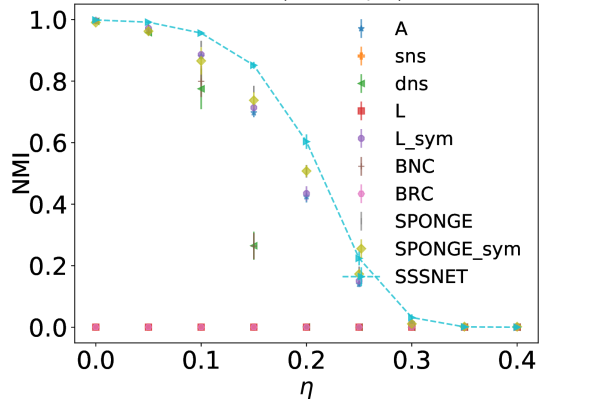
(a) NMI of SSBM($n=30000,K=5,p=0.001,\rho=1.5$)

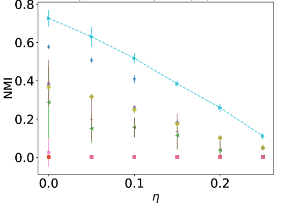
(b) NMI of Pol-SSBM($n=10000,n_{c}=2,p=0.01,\rho=1.5$)

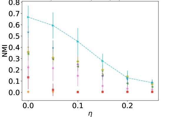
(c) NMI of
Pol-SSBM($n=1050,n_{c}=2,p=0.1,\rho=1$)

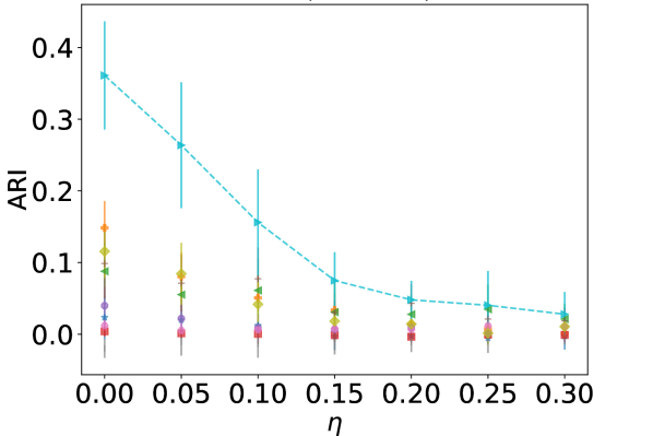
(d) ARI of SSBM($n=1000,K=20,p=0.01,\rho=1.5$)

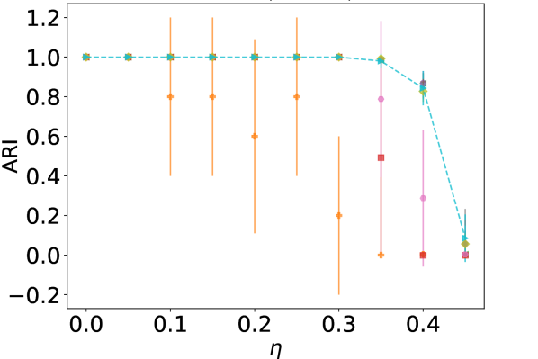
(e) ARI of
SSBM($n=1000,K=2,p=0.1,\rho=2$)

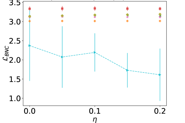
(f) $\mathcal{L}_{\text{BNC}}$ of Pol-SSBM($n=5000,n_{c}=3,p=0.1,\rho=1.5$)

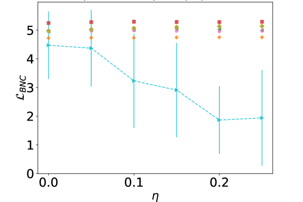
(g) $\mathcal{L}_{\text{BNC}}$ of Pol-SSBM($n=5000,n_{c}=5,p=0.1,\rho=1.5$)

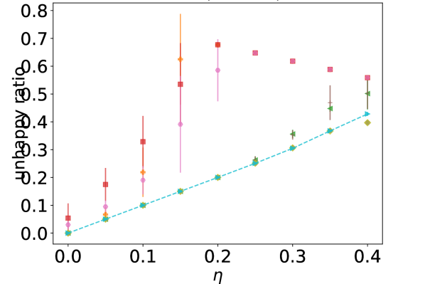
(h) Unhappy ratio of SSBM($n=10000,K=5,p=0.01,\rho=1.5$)

Figure 6: Extended node clustering result comparison on synthetic data. Dashed lines are added to SSSNET’s performance to highlight our result. Each setting is averaged over ten runs. Error bars are given by standard errors. NMI and ARI results are on test nodes only (the higher, the better), while $\mathcal{L}_{\text{BNC}}$ and unhappy ratio results are on all nodes in the signed network (the lower, the better).

From Figure 6, we remark that SSSNET gives comparable balanced normalized cut values and unhappy ratios in these regimes, and leading performance in terms of both ARI and NMI.

A.2 Additional Results on Real-World Data

A.2.1 Discussion on Attributes for Sampson

On this data set, SSSNET with the ‘Cloisterville’ attribute achieves highest ARI. When ignoring this attribute and instead using the identity matrix with 25 rows as input feature matrix for Sampson, we achieve a test ARI 0.37$\pm$0.19, which is much lower than SSSNET’s test ARI with 1-dimensional attributes, but still higher than the other methods.

A.2.2 Extended Result Table for Fin-YNet

Table 3 gives an extended comparison of different methods on the financial correlation data set Fin-YNet. In the first panel of table the difference ($\pm$ 1 s.e. when applicable) to the best-performing method is given; hence each row will have at least one zero entry.

Table 3: Clustering performance comparison on Fin-YNet; the first panel shows distance to the best performance and the second panel shows absolute performance. The best is in bold red, and second best in underline blue. Standard deviations are not shown due to space constraint.

Metric	A	sns	dns	L	L_sym	BNC	BRC	SPONGE	SPONGE_sym	SSSNET
test ARI dist.	0.22	0.37	0.32	0.33	0.22	0.32	0.33	0.20	0.16	0.00
all ARI dist.	0.27	0.43	0.37	0.38	0.27	0.37	0.38	0.24	0.2	0.00
test NMI dist.	0.11	0.53	0.39	0.39	0.14	0.39	0.40	0.12	0.09	0.00
all NMI dist.	0.17	0.44	0.35	0.36	0.19	0.35	0.35	0.12	0.11	0.00
test ARI	0.18	0.03	0.08	0.07	0.17	0.08	0.07	0.19	0.24	0.40
all ARI	0.19	0.03	0.09	0.08	0.19	0.09	0.08	0.22	0.26	0.46
test NMI	0.54	0.12	0.26	0.26	0.51	0.26	0.25	0.53	0.56	0.65
all NMI	0.38	0.11	0.20	0.19	0.36	0.20	0.19	0.42	0.44	0.55

We conclude that SSSNET attains the best performance in terms of both ARI and NMI, with regards to both test nodes and all nodes, in each of the 21 years.

A.2.3 GICS Alignments Plots on S&P1500

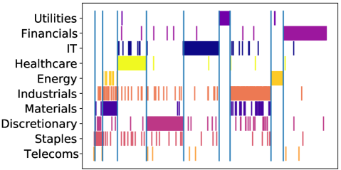
Figure 7: Alignment of SSSNET clusters with GICS sectors in S&P 1500; ARI=0.71. Colors denote distinct sectors of the US economy, indexing the rows; the total area of a color denotes the size of a GICS sector. Columns index the recovered SSSNET clusters, with the widths proportional to cluster sizes.

We remark that SSSNET (Figure 7) uncovers several very cohesive clusters, such as IT, Discretionary, Utility, and Financials. These recovered clusters are visually more cohesive than those reported by SPONGE.

B Extended Data Description

B.1 SSBM Construction Details

A Signed Stochastic Block Model (SSBM) for a network on $n$ nodes with $K$ blocks (clusters), is constructed similar to [14] but with a more general cluster size definition.

$\bullet$(1) Assign block sizes $n_{0}\leq n_{1}\leq\cdots\leq n_{K-1}$ with size ratio $\rho\geq 1$, as follows. If $\rho=1$, then the first $K-1$ blocks have the same size $\lfloor n/K\rfloor$, and the last block has size $n-(K-1)\lfloor n/K\rfloor$. If $\rho>1$, we set $\rho_{0}=\rho^{\frac{1}{K-1}}.$ Solving $\sum_{i=0}^{K-1}\rho_{0}^{i}n_{0}=n$ and taking integer value gives $n_{0}=\left\lfloor{n(1-\rho_{0})}/{(1-\rho_{0}^{K})}\right\rfloor.$ Further, set $n_{i}=\lfloor\rho_{0}n_{i-1}\rfloor,$ for $i=1,\cdots,K-2$ if $K\geq 3,$ and $n_{K-1}=n-\sum_{i=0}^{K-2}n_{i}.$ Then, the ratio of the size of the largest to the smallest block is approximately $\rho_{0}^{K-1}=\rho.$ $\bullet$(2) Assign each node to one of $K$ blocks, so that each block has the allocated size. $\bullet$(3) For each pair of nodes in the same block, with probability $p_{\text{in}}=p$, create an edge with $+1$ as weight between them, independently of the other potential edges. $\bullet$(4) For each pair of nodes in different blocks, with probability $p_{\text{out}}=p,$ create an edge with $-1$ as weight between them, independently of the other potential edges. $\bullet$(5) Flip the sign of the across-cluster edges from the previous stage with sign flip probability $\eta_{\text{in}}=\eta$, and $\eta_{\text{out}}=\eta$ for edges within and across clusters, respectively.

As our framework can be applied to different connected components separately, after generating the initial SSBM, we concentrate on the largest connected component. To further avoid numerical issues, we modify the synthetic network by adding randomly wired edges to nodes of degree 1 or 2.

The actual implementation of the above algorithm is given in https://github.com/SherylHYX/SSSNET_Signed_Clustering/blob/main/src/utils.py, modified from https://github.com/alan-turing-institute/SigNet/blob/master/signet/block_models.py.

B.2 Discussion on POL-SSBM

Our generalizations are as follows: $\bullet$(1) Our model allows for different sizes of communities and blocks, governed by the parameter $\rho$, which is more realistic. $\bullet$(2) Instead of using a single parameter for the edge probability and sign flips, we use two parameters $p$ and $\eta$. We also assume equal edge sampling probability throughout the entire graph, as we want to avoid being able to trivially solve the problem by considering the absolute value of the edge weights, and thus falling back onto the standard community detection setting in unsigned graphs. $\bullet$(3) We consider more than two polarized communities, while also allowing for the existence of ambient nodes in the graph, in the spirit of [54].

B.3 Real-World Data Description

We perform experiments on six real-world signed network data sets (Sampson [43], Rainfall [5], Fin-YNet, S&P 1500 [56], PPI [50], and Wiki-Rfa [53]). Table 1 in the main text gives some summary statistics; here is a brief description of each data set.

$\bullet$The Sampson monastery data [43] were collected by Sampson while resident at the monastery; the study spans 12 months. This data set contains relationships (esteem, liking, influence, praise, as well as disesteem, negative influence, and blame) between 25 novices in total, who were preparing to join a New England monastery. Each novice was asked to rank their top three choices for each of these relationships. Some novices gave ties for some of the choices, and nominated four instead of three other novices. the positive attributes have values 1, 2 and 3 in increasing order of affection, whereas the negative attributes take values -1, -2, and -3, in increasing order of dislike. The social relations were measured at five points in time. Some novices had left the monastery during this process; at time point 4, 18 novices are present. These novices possess as feature whether or not they attended the minor seminary of ‘Cloisterville’ before coming to the monastery. For the other 7 novices this information is not available. We combine these relationships into a network of 25 nodes by adding the weights for each relationship across all time points. Missing observations were set to 0. Based on his observations and analyses, Sampson divided the novices into four groups: Young Turks, Loyal Opposition, Outcasts, and an interstitial group; this division is taken as ground truth. We use as node (novice) attribute whether or not they attended ‘Cloisterville’ before coming to the monastery.

$\bullet$Rainfall [5] contains 64,408 pairwise correlations between $n=306$ locations in Australia, at which historical rainfalls have been measured.

$\bullet$Fin-YNet consists of yearly correlation matrices for $n=451$ stocks for 2000-2020 (21 distinct networks), using market excess returns. That is, we compute each correlation matrix from overnight (previous close to open) and intraday (open-to-close) price daily returns, from which we subtract the market return of the S&P500 index for the same time interval. In other words, within a given year, for each stock, we consider the time series of 500 market excess returns (there are 250 trading days within a year, and each day contributes with two returns, an overnight one and in intraday one). Each correlation network is built from the empirical correlation matrix of the entire set of stocks. For this data set, we report the results averaged over the 21 networks.

$\bullet$S&P1500 [56] considers daily prices for $n=1,193$ stocks in the S&P 1500 Index, between 2003 and 2015, and builds correlation matrices from market excess returns (ie, from the return price of each financial instrument, the return of the market S&P500 is subtracted). Since we do not threshold, the result is thus a fully-connected weighted network, with stocks as nodes and correlations as edge weights.

$\bullet$PPI [50] is a signed protein-protein interaction network between $n=3,058$ proteins.

$\bullet$Wiki-Rfa [53] is a signed network describing voting information for electing Wikipedia managers. Positive edges represent supporting votes, while negative edges represent opposing votes. We extract the largest connected component and remove nodes with degree at most one, resulting in $n=7,634$ nodes for experiments.

C Implementation Details

C.1 Efficient Algorithm for SIMPA

An efficient implementation of SIMPA is given in Algorithm 1. We omit the subscript $\mathcal{V}$ for ease of notation. The matrix operations described in Eq. (3.1) in the main text appear to be computationally expensive and space unfriendly. However, SSSNET resolves these concerns via an efficient sparsity-aware implementation without explicitly calculating the sets of powers, such as $\mathcal{A}^{s+,h}.$ The algorithm also takes sparse matrices as input, and sparsity is maintained throughout. Therefore, for input feature dimension $d_{\text{in}}$ and hidden dimension $d$, if $d^{\prime}=\max(d_{\text{in}},d)\ll n,$ time and space complexity of SIMPA, and implicitly SSSNET, is $\mathcal{O}(|\mathcal{E}|d^{\prime}h^{2}+4nd^{\prime}K)$ and $\mathcal{O}(4|\mathcal{E}|+10nd^{\prime}+nK),$ respectively [23, 19]. When the network is large, SIMPA is amendable to a minibatch version using neighborhood sampling, similar to the minibatch forward propagation algorithm in [21, 37]. SIMPA is also amenable to an auto-scale version with theoretical guarantees, following [18].

Input : (Sparse) row-normalized adjacency matrices $\overline{\mathbf{A}}^{s+},\overline{\mathbf{A}}^{s-},\overline{\mathbf{A}}^{t+},\overline{\mathbf{A}}^{t-}$; initial hidden representations $\mathbf{H}^{s+},\mathbf{H}^{s-},\mathbf{H}^{t+},\mathbf{H}^{t-}$; hop $h$; lists of scalar weights $\Omega^{s+}=(\omega_{\mathbf{M}}^{s+},\mathbf{M}\in\mathcal{A}^{s+,h}),\Omega^{s-}=(\omega_{\mathbf{M}}^{s-},\mathbf{M}\in\mathcal{A}^{s-,h}),$ $\Omega^{t+}=(\omega_{\mathbf{M}}^{t+},\mathbf{M}\in\mathcal{A}^{t+,h}),\Omega^{t-}=(\omega_{\mathbf{M}}^{t-},\mathbf{M}\in\mathcal{A}^{t-,h}).$

Output : Vector representations $\mathbf{z}_{i}$ for all $v_{i}\in\mathcal{V}$ given by $\mathbf{Z}.$

$\mathbf{Z}^{s+}\leftarrow\Omega^{s+}[0]\cdot\mathbf{H}^{s+}$; $\mathbf{Z}^{t+}\leftarrow\Omega^{t+}[0]\cdot\mathbf{H}^{t+}$; $\mathbf{Z}^{s-},\mathbf{Z}^{t-}\leftarrow\mathbf{0}$;

$\tilde{\mathbf{X}}^{s+}\leftarrow\mathbf{H}^{s+},\bar{\mathbf{X}}^{s-}\leftarrow\mathbf{H}^{s-},\tilde{\mathbf{X}}^{t+}\leftarrow\mathbf{H}^{t+},\bar{\mathbf{X}}^{t-}\leftarrow\mathbf{H}^{t-}$; $j\leftarrow 0$;

for $i\leftarrow 0$ to $h$ do

       if $i>0$ then

             $\tilde{\mathbf{X}}^{s+}\leftarrow\overline{\mathbf{A}}^{s+}\tilde{\mathbf{X}}^{s+}$; $\tilde{\mathbf{X}}^{t+}\leftarrow\overline{\mathbf{A}}^{t+}\tilde{\mathbf{X}}^{t+}$ ;

             $\mathbf{Z}^{s+}\leftarrow\mathbf{Z}^{s+}+\Omega^{s+}[i]\cdot\tilde{\mathbf{X}}^{s+}$; $\bar{\mathbf{X}}^{s-}\leftarrow\overline{\mathbf{A}}^{s+}\bar{\mathbf{X}}^{s-}$;

             $\mathbf{Z}^{t+}\leftarrow\mathbf{Z}^{t+}+\Omega^{t+}[i]\cdot\tilde{\mathbf{X}}^{t+}$; $\bar{\mathbf{X}}^{t-}\leftarrow\overline{\mathbf{A}}^{t+}\bar{\mathbf{X}}^{t-}$;

       end if

      if $i\neq h$ then

             $\tilde{\mathbf{X}}^{s-}\leftarrow\overline{\mathbf{A}}^{s-}\bar{\mathbf{X}}^{s-}$; $\tilde{\mathbf{X}}^{t-}\leftarrow\overline{\mathbf{A}}^{t-}\tilde{\mathbf{X}}^{t-}$ ;

             $\mathbf{Z}^{s-}\leftarrow\mathbf{Z}^{s-}+\Omega^{s-}[j]\cdot\tilde{\mathbf{X}}^{s-}$;

             $\mathbf{Z}^{t-}\leftarrow\mathbf{Z}^{t-}+\Omega^{t-}[j]\cdot\tilde{\mathbf{X}}^{t-}$; $j\leftarrow j+1$;

             for $k\leftarrow 0$ to $h-i-2$ do

                   $\tilde{\mathbf{X}}^{s-}\leftarrow\overline{\mathbf{A}}^{s+}\bar{\mathbf{X}}^{s-}$; $\tilde{\mathbf{X}}^{t-}\leftarrow\overline{\mathbf{A}}^{t+}\tilde{\mathbf{X}}^{t-}$ ;

                   $\mathbf{Z}^{s-}\leftarrow\mathbf{Z}^{s-}+\Omega^{s-}[j]\cdot\tilde{\mathbf{X}}^{s-}$;

                   $\mathbf{Z}^{t-}\leftarrow\mathbf{Z}^{t-}+\Omega^{t-}[j]\cdot\tilde{\mathbf{X}}^{t-}$; $j\leftarrow j+1$;

                  

             end for

            

       end if

      

end for

$\mathbf{Z}=\operatorname{CONCAT}\left(\mathbf{Z}^{s+},\mathbf{Z}^{s-},\mathbf{Z}^{t+},\mathbf{Z}^{t-}\right)$;

Algorithm 1 Signed Mixed-Path Aggregation (SIMPA) algorithm for signed directed networks

C.2 Machines

Experiments were conducted on a compute node with 4 Nvidia RTX 8000, 48 Intel Xeon Silver 4116 CPUs and $1000$GB RAM, a compute node with 3 NVIDIA GeForce RTX 2080, 32 Intel Xeon E5-2690 v3 CPUs and $64$GB RAM, a compute node with 2 NVIDIA Tesla K80, 16 Intel Xeon E5-2690 CPUs and $252$GB RAM, and an Intel 2.90GHz i7-10700 processor with 8 cores and 16 threads. With the above, most experiments can be completed within a day.

C.3 Data Splits and Input

For each setting of synthetic data and real-world data, we first generate five different networks, each with two different data splits, then conduct experiments on them and report average performance over these 10 runs.

For synthetic data, 10% of all nodes are selected as test nodes for each cluster (the actual number is the ceiling of the total number of nodes times 0.1, so we would not fall below 10% of test nodes), 10% are selected as validation nodes (for model selection and early-stopping; again, we take the ceiling for the actual number), while the remaining roughly 80% are selected as training nodes (the actual number is bounded above by 80% since we take ceiling). For most real-world data sets, we extract the largest weak connected component for experiments. For Wiki-Rfa, we further rule out nodes that have degree less than two.

As for input features, we weigh the unit-length eigenvectors of the Signed Laplacian or regularized adjacency matrix by their eigenvalues introduced in [25]. For the Signed Laplacian features, we divide each eigenvector by its corresponding eigenvalue, since smaller eigenvectors are more likely to be informative. For regularized adjacency matrix features, we multiply eigenvalues by eigenvectors, since larger eigenvectors are more likely to be informative. After this scaling, there are no further standardization steps before inputting the features to our model. When features are available (in the case of Sampson data set), we standardize the one-dimensional binary input feature, so that the whole vector has mean zero and variance one.

For the sns and dns methods defined in Sec. 4.2 in the main text, we stack the eigenvectors associated with the smallest $K$ eigenvalues of the corresponding Laplacians [58] to construct the feature matrix, then apply K-means to obtain the cluster assignments. For the other implementations, we also take the first $K$ eigenvectors, either smallest or largest, following https://github.com/alan-turing-institute/SigNet/blob/master/signet/cluster.py.

C.4 Hyperparameters

We conduct hyperparmeter selection via a greedy search manner. To explain the details, consider for example the following synthetic data setting: polarized SSBMs with 1050 nodes, $n_{c}=2$ SSBM communities, $\rho=1.5,N=200,p=0.1.$

Recall that the the objective function minimizes

(C.1) $$\mathcal{L}=\mathcal{L}_{\text{PBNC}}+\gamma_{s}(\mathcal{L}_{\text{CE}}+\gamma_{t}\mathcal{L}_{\text{triplet}}),$$

where $\gamma_{s},\gamma_{t}>0$ are weights for the supervised part of the loss and triplet loss within the supervised part, respectively.

Note that the cosine similarity (used in triplet loss $\mathcal{L}_{\text{triplet}}$) between two randomly picked vectors in $d$ dimensions is bounded by $\sqrt{\ln(d)/d}$ with high probability. In our experiments $d=32$, and $\sqrt{\ln(2d)/(2d)}\approx 0.25,\sqrt{\ln(4d)/(4d)}\approx 0.19.$ In contrast, for fairly uniform clustering, the cross-entropy loss grows like $\log n$, which in our experiments ranges between 3 and 17. Thus some balancing of the contribution is required.

Instead of a grid search, we tune hyperparameters according to what performs the best in the current default setting. If two settings give similar results, we pick the simpler setting, for example, the smaller hop size or the lower number of seed nodes.

When we reach a local optimum, we stop searching. Indeed, just a few iterations (less than five) were required for us to find the current setting, as SSSNET tends to be robust to most hyperparameters.

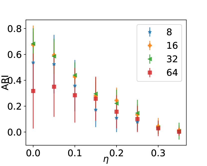
(a) Vary $d$, the MLP hidden dimension

.

(b) Vary $h$, the number of hops for aggregation

.

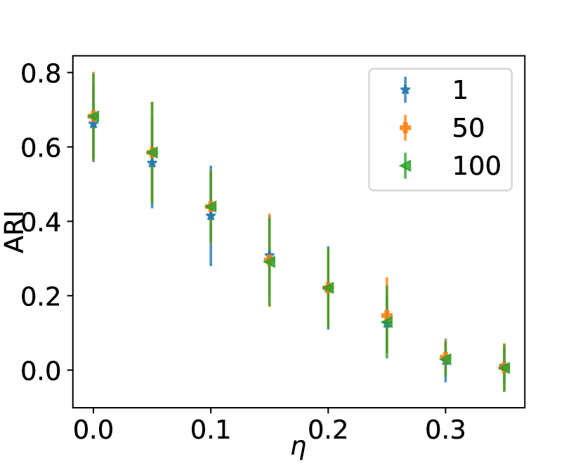
(c) Vary $\tau$, weight of the added self-loop to $\mathbf{A}^{+}$

.

(d) Vary $\gamma_{s}$ in Eq. (3.4) in main.

(e) Vary $\gamma_{t}$ in Eq. (3.4) in main.

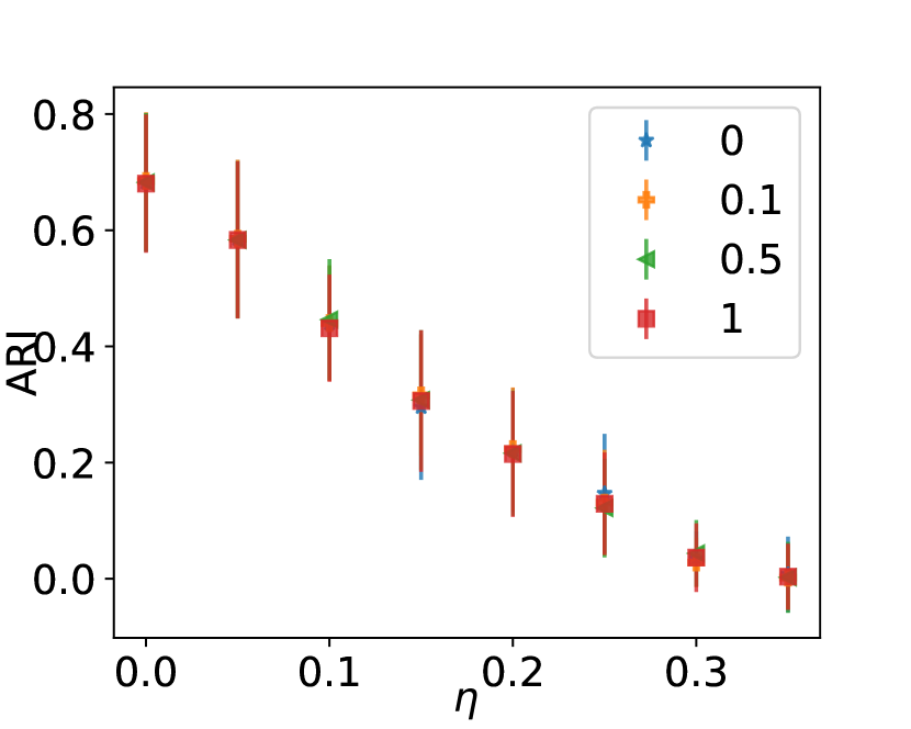
(f) Vary $\alpha$ in $\mathcal{L}_{\text{triplet}}$.

Figure 8: Hyperpameter analysis on polarized SSBMs with $n=1050$ nodes, $n_{c}=2$ communites, $\rho=1.5,$ default community size $N=200$, and $p=0.1.$

Figure 8 compares the performance of SSSNET on polarized SSBMs with 1050 nodes, $n_{c}=2$ SSBM communities, $\rho=1.5,N=200,p=0.1,$ under different hyperparameter settings. By default, we use the loss function Eq. (3.4) in the main text with $\gamma_{t}=0.1,\gamma_{s}=50,$ and $d=32,l=2,\tau=0.5,h=2,\alpha=0.$ We use the default seed ratio as 0.1 (the ratio of the number of seed nodes to the number of training nodes). We remark from (a) that as we increase the MLP hidden dimension $d$, performance first improves then decreases, with 32 a desirable value. As we increase the number of hops to consider, performance drops in (b). Therefore, we would use the simplest, yet best choice, hop 2. The decrease in both cases might be explained by too much noise introduced. For (c), the self-loop weight $\tau$ added to the positive part of the adjacency matrix does not seem to affect performance much, and hence we use 0.5 throughout. We conclude from (d) that it is recommended to have $\gamma_{s}>1$ so as to take advantage of labeling information. The best triplet loss ratio in our candidates is $\gamma_{t}=0.1$, based on (e). From (f), the influence of $\alpha$ is not evident, and hence we use $\alpha=0$ throughout.

C.5 Training

For all synthetic data, we train SSSNET with a maximum of 300 epochs, and stop training when no gain in validation performance is achieved for 100 epochs (early-stopping).

For real-world data, when “ground-truth” labels are available, we still have separate test nodes. For S&P1500 data set, we do not have validation nodes, and 90% of all nodes are training nodes. For data sets with no “ground-truth” labels available, we train SSSNET in a self-supervised setting, using all nodes to train. We stop training when the training loss does not decrease for 100 epochs or when we reach the maximum number of epochs, 300.

For the two-layer MLP, we do not have a bias term for each layer, and we use a Rectified Linear Unit (ReLU), followed by a dropout layer with 0.5 dropout probability between the two layers, following [48]. We use Adam as the optimizer, and $\ell_{2}$ regularization with weight decay $5\cdot 10^{-4}$ to avoid overfitting.

C.6 Aggregation Matrices

In practice, in order not to consider $h-$hop neighbors that are “fake” (due to added self-loops), after obtaining the aggregation matrix in Sec. 3.3.1, for example, a matrix from $\mathcal{A}^{s-,h}=\left\{(\mathbf{\overline{A}}^{s+})^{h_{1}}\cdot\mathbf{\overline{A}}^{s-}\cdot(\mathbf{\overline{A}}^{s+})^{h_{2}}:h_{1},h_{2}\in H\right\}$, we set the entries that should not be nonzero if we do not add self-loops to zero. In other words, we only keep entries that exist in $(\mathbf{{A}}^{+})^{h_{1}}\cdot\mathbf{A}^{-}\cdot(\mathbf{A}^{+})^{h_{2}}$ for $h_{1},h_{2}\in H.$ This trick originates from the implementation of [48].

References

- [1] S. Aghabozorgi et al. Time-series clustering–a decade review. Information Systems, 53:16–38, 2015.
- [2] A. Amelio and C. Pizzuti. Is normalized mutual information a fair measure for comparing community detection methods? In ASONAM, 2015.
- [3] A. Amini et al. Pseudo-likelihood methods for community detection in large sparse networks. The Annals of Statistics, 41(4):2097–2122, 2013.
- [4] M. Arfaoui and A. Rejeb. Oil, gold, us dollar and stock market interdependencies: a global analytical insight. European Jour. of Management and Business Economics, 26:278–293, 2017.
- [5] M. Bertolacci et al. Climate inference on daily rainfall across the Australian continent, 1876–2015. Annals of Applied Statistics, 13(2):683–712, 2019.
- [6] K. Bhowmick et al. On the network embedding in sparse signed networks. In Lec. Notes in CS, volume 11441, pages 94–106, China, 2019. Springer Verlag.
- [7] F. Bonchi et al. Discovering polarized communities in signed networks. In CIKM. ACM, 2019.
- [8] K. Chaudhuri et al. Spectral clustering of graphs with general degrees in the extended planted partition model. In 25th COLT, 2012.
- [9] X. Chen et al. Decoupled variational embedding for signed directed networks. TWEB, 15(1), 2020.
- [10] Y. Chen et al. BASSI: Balance and status combined signed network embedding. In Lec. Notes in CS, volume 10827, pages 55–63. Springer Verlag, 2018.
- [11] Y. Chen et al. ”Bridge”: Enhanced Signed Directed Network Embedding. In CIKM, 2018.
- [12] K. Chiang et al. Scalable clustering of signed networks using balance normalized cut. In CIKM, 2012.
- [13] M. Cucuringu et al. Scalable Constrained Clustering: A Generalized Spectral Method. AISTATS, 2016.
- [14] M. Cucuringu et al. SPONGE: A generalized eigenproblem for clustering signed networks. In AISTATS, 2019.
- [15] M. Cucuringu et al. Regularized spectral methods for clustering signed networks. arXiv:2011.01737, 2020.
- [16] M. Cucuringu et al. An MBO scheme for clustering and semi-supervised clustering of signed networks. Communications in Mathematical Sciences, 19(1):73–109, 2021.
- [17] T. Derr et al. Signed graph convolutional networks. In ICDM, Singapore, 2018. IEEE.
- [18] M. Fey et al. GNNAutoScale: Scalable and expressive graph neural networks via historical embeddings. In ICML, 2021.
- [19] G. Greiner and R. Jacob. The I/O complexity of sparse matrix dense matrix multiplication. In Latin American Symposium on Theoretical Informatics, pages 143–156. Springer, 2010.
- [20] R. Guha et al. Propagation of trust and distrust. In WWW, 2004.
- [21] W. Hamilton et al. Inductive representation learning on large graphs. In NeurIPS, 2017.
- [22] F. Harary. On the notion of balance of a signed graph. Michigan Mathematical Journal, 2(2):143–146, 1953.
- [23] A. Harrison and D. Joseph. High performance rearrangement and multiplication routines for sparse tensor arithmetic. SIAM Jour. on Scientific Computing, 40(2):C258–C281, 2018.
- [24] Y. He et al. PyTorch Geometric Signed Directed: A Survey and Software on Graph Neural Networks for Signed and Directed Graphs. arXiv preprint arXiv:2202.10793, 2022.
- [25] Y. Hou et al. On the laplacian eigenvalues of signed graphs. Linear and Multilinear Algebra, 51(1), 2003.
- [26] J. Huang et al. Signed Graph Attention Networks. In Lec. Notes in CS. Springer Verlag, 2019.
- [27] J. Huang et al. SDGNN: Learning Node Representation for Signed Directed Networks. arXiv:2101.02390, 2021.
- [28] Lawrence Hubert and Phipps Arabie. Comparing partitions. Jour. of Classification, 2(1):193–218, 1985.
- [29] A. Javari et al. ROSE: Role-based Signed Network Embedding. In WWW. ACM, 2020.
- [30] A. Jha et al. Clustering to forecast sparse time-series data. In ICDE. IEEE, 2015.
- [31] T. Kipf and M. Welling. Semi-supervised classification with graph convolutional networks. ICLR, 2017.
- [32] J. Kunegis et al. Spectral analysis of signed graphs for clustering, prediction and visualization. In ICDM, Sydney, Australia, 2010. SIAM, IEEE.
- [33] Y. Lee et al. ASiNE: Adversarial Signed Network Embedding. In SIGIR. ACM, 2020.
- [34] J. Leskovec et al. Signed networks in social media. In SIGCHI. ACM, 2010.
- [35] Y. Li et al. Learning signed network embedding via graph attention. In AAAI, 2020.
- [36] X. Liu et al. Semi-supervised stochastic blockmodel for structure analysis of signed networks. Knowledge-Based Systems, 195:105714, 2020.
- [37] E. Markowitz et al. Graph traversal with tensor functionals: A meta-algorithm for scalable learning. In ICLR, 2021.
- [38] P. Mercado et al. Clustering signed networks with the geometric mean of laplacians. In NeurIPS, 2016.
- [39] A. Patidar et al. Predicting friends and foes in signed networks using inductive inference and social balance theory. In ASONAM. IEEE, 2012.
- [40] K. Read. Cultures of the central highlands, New Guinea. Southwestern Jour. of Anthropology, 10(1):1–43, 1954.
- [41] M. Riolo et al. Efficient method for estimating the number of communities in a network. Physical Review E, 96(3):032310, 2017.
- [42] S. Romano et al. Standardized mutual information for clustering comparisons: one step further in adjustment for chance. In ICML. PMLR, 2014.
- [43] S. Sampson. A novitiate in a period of change: An experimental and case study of social relationships (PhD thesis). Cornell University, USA, 1968.
- [44] K. Sharma et al. Balance maximization in signed networks via edge deletions. In WSDM, 2021.
- [45] Xing Su et al. A comprehensive survey on community detection with deep learning. arXiv preprint arXiv:2105.12584, 2021.
- [46] J. Tang et al. Is distrust the negation of trust? the value of distrust in social media. In ACMHT, 2014.
- [47] J. Tang et al. Recommendations in signed social networks. In WWW, 2016.
- [48] Y. Tian et al. Rethinking kernel methods for node representation learning on graphs. NeurIPS, 2019.
- [49] R. Tzeng et al. Discovering conflicting groups in signed networks. NeurIPS, 33, 2020.
- [50] A. Vinayagam et al. Integrating protein-protein interaction networks with phenotypes reveals signs of interactions. Nature Methods, 11(1):94–99, 2014.
- [51] S. Wang et al. Attributed Signed Network Embedding. In CIKM. ACM, 2017.
- [52] S. Wang et al. Signed network embedding in social media. In ICDM. SIAM, 2017.
- [53] R. West et al. Exploiting social network structure for person-to-person sentiment analysis. TACL, 2, 2014.
- [54] H. Xiao et al. Searching for polarization in signed graphs: a local spectral approach. WWW, 2020.
- [55] P. Xu et al. Social trust network embedding. In ICDM, volume 2019, 2019.
- [56] yahoo! finance. S&p 1500 data. https://finance.yahoo.com/, 2021. [Online; accessed 19-January-2021].
- [57] D. Yan et al. Muse: Multi-faceted attention for signed network embedding. arXiv:2104.14449, 2021.
- [58] Q. Zheng and D. Skillicorn. Spectral embedding of signed networks. In ICDM. SIAM, 2015.