Phase Curves of Small Bodies from the SLOAN Moving Objects Catalog

Abstract

Context. Extensive photometric surveys are and will continue producing massive amounts of data on small bodies. Usually, these data will be sparsely obtained at arbitrary (and unknown)rotational phases. Therefore, new methods to process such data need to be developed to make the most of those large catalogs.

Aims. We aim to produce a method to create phase curves of small bodies considering the uncertainties introduced by the nominal errors in the magnitudes and the effect introduced by rotational variations.

We use the SLOAN Moving Objects Catalog data as a benchmark to construct phase curves of all small bodies in there, in u’, g’, r’, i’, and z’ filters. We will obtain from the phase curves the absolute magnitudes and set up with them the absolute colors, which are the colors of the asteroids not affected by changes in phase angle.

Methods. We select objects with $\geq 3$ observations taken in at least one filter and spanned over a minimum of 5 degrees in phase angle. We developed a method that combines Monte Carlo simulations and Bayesian inference to estimate the absolute magnitudes using the HG${}_{12}^{*}$ photometric system.

Results. We obtained almost 15 000 phase curves, about 12 000 including all five filters. The absolute magnitudes and absolute colors are compatible with previously published data, supporting our method.

Conclusions. The method we developed is fully automatic and well suited to be run on large amounts of data. Moreover, it includes the nominal uncertainties in the magnitudes and the whole distribution of possible rotational states of the objects producing, possibly, less precise values, i.e., larger uncertainties, but more accurate, i.e., closer to the actual value. To our knowledge, this work is the first to include the effect of rotational variations in such a manner.

1 Introduction

The field of modern planetary sciences is experiencing a revolution due to: (1) Space missions to targets of interest and (2) massive databases produced as outcomes from extensive observational surveys. As far as item (1) is concerned, we will only mention that, although extremely useful, space missions provide detailed information about a handful of objects. However, these data are used to impose constraints on whole populations [for instance 67P, visited by ESA’s Rosetta mission (Barucci & Fulchignoni, 2017, and references therein), or JAXA’s Hayabusa visit to Itokawa (Fujiwara et al., 2006, and references therein) it is like admiring a painting at a very close range. On the other hand, extensive observational surveys produce large amounts of data, which allow us to study whole populations, their distribution in the observational parameters space, or relations, while being more difficult to obtain detailed information about individual objects, usually because most of them would only be observed once or twice. This is like admiring a painting from a distance, recognizing its patterns but not the details of the strokes. We present a method to make the most of data provided by large observational surveys in this work.

Among the future and ongoing surveys, some of them will produce multi-wavelength photometric catalogs. Two examples are, first, the future Legacy Survey of Space and Time (LSST) to be executed by the Vera C. Rubin Observatory, which will observe massive numbers of small bodies (Jones et al., 2009), and the already published MOVIS catalog that gathers near-infrared magnitudes of small bodies from the VISTA-VHS survey (Popescu et al., 2016). In particular, for the scope of the present work, we are interested in two specific surveys: The Javalambre Physics of the Accelerating Universe, J-PAS (Benitez et al., 2014) that will observe 8 000 sq degrees of the northern sky in 56 different filters (54 narrowband and two broadband) using a 2.5-m telescope and the Javalambre Photometric Local Universe Survey, J-PLUS (Cenarro et al., 2019) that is observing the same footprint as J-PAS but with 12 filters (5 broadband) using a 0.8-m telescope. The power of these surveys relies not only on the large footprint but also on the number of filters to be used for the observations, which provides unprecedented spectral coverage for spectro-photometry (see Morate et al., 2021, for an example on J-PLUS data of asteroids). Unfortunately, the data are taken sparsely due to the observational strategy, and different filters may be observed at different epochs. Therefore, new methods need to be developed to make these data useful for small bodies.

Aiming at providing one such tool, we develop a method that combines Monte Carlo simulations and Bayesian inference to include the effect of rotational variation between different epochs. As a test, and also because of its importance in the study of small bodies, we concentrate on data produced by the SLOAN Digital Survey (York et al., 2000), whose photometric survey produced detection of several thousand moving objects, many of them linked to real objects in their Moving Objects Catalog (hereafter just MOC, Ivezić et al., 2001; Jurić et al., 2002). The MOC data have been widely used to characterize diverse populations of asteroids, comets, and trans-Neptunian objects (TNOs). Some applications have been the taxonomical classification of small bodies and the study of the mass distribution in the Main Belt of asteroids (for example: Roig & Gil-Hutton, 2006; Roig et al., 2008; Gil-Hutton & Brunini, 2008; Assandri & Gil-Hutton, 2008; Gil-Hutton & Licandro, 2010; Carvano et al., 2010; Solontoi et al., 2010; Ofek, 2012; Solontoi et al., 2012; Alvarez-Candal, 2013; DeMeo & Carry, 2013, 2014; Hasselmann et al., 2015; Carry et al., 2016, and others). In particular, we concentrate on those objects that appear multiple times in the MOC ($>15\,000$ with at least three different observations) in any of the five filters of the SLOAN photometric system. We aim at constructing their phase curves in all filters used by the survey, providing a catalog of zero-phase magnitudes or absolute magnitudes. This work does not aim to perform an in-depth analysis of the results but to provide the community with a valuable set of data to be further studied.

The absolute magnitude, $H$, of an airless small body is defined as the object’s apparent magnitude if illuminated by the Sun at 1 AU while being observed from a distance of 1 AU at opposition. The importance of $H$ comes from its well-known relation with the size of the object and its albedo (Bowell & Lumme, 1979). $H$ is computed using phase curves (PCs hereafter) which relate the change of the apparent magnitudes with the phase angle ($\alpha$, which is the angular distance between the Sun and the Earth as seen from the object). Due to the characteristics of the PCs, it is necessary to (i) have observations at several different $\alpha$, and (ii) to take into account the effect of the rotational variability. Therefore, a PC usually cannot be constructed with data of only one observational run (spanning just a few nights), except for Near Earth Objects (NEOs), because there may not be enough coverage in $\alpha$. Note that possible changes in brightness due to different apparitions (aspect angle-related) should also be included. Nevertheless, this issue will not be tackled in this work.

Two different approaches can be used to create PCs. On the one hand, targeted observations of selected objects, with dedicated telescope (or telescopes) time (Carbognani et al., 2019, among others). This approach has obvious advantages: target selection, enough time to remove rotational variation (we will come back to this in Sect. 3), and control over the overall observational setup (i.e., filter selection, range of $\alpha$, etc.) On the downside, these observations can demand many telescope hours and careful planning to have maximum efficiency. On the other hand, it is possible to use the large amount of data produced by several extensive observational surveys (on-going and future). Key references in this regard are the almost half a million absolute magnitudes from the Minor Planets Center compiled by Oszkiewicz et al. (2011), the 250 000 Pan-STARRS absolute magnitudes (Vereš et al., 2015), the analysis of almost 100 000 asteroids from the ATLAS survey (Mahlke et al., 2021), or the almost 15 000 PCs from Gaia Data Release 2 (DR2) observations (Colazo et al., 2021). This second approach has no control over the observational setup or target selection, and all work should be executed on serendipitous observations. The advantage relies on massive numbers, several orders of magnitude larger than anything that can be done with targeted studies.

We aim in this work at constructing all possible PCs from the MOC for objects with at least three observations (different $\alpha$, and with a minimum spread of 5 degrees) in any of the filters. We obtain absolute magnitudes of several thousand objects that allow constructing colors at $\alpha=0$ degrees, i.e., not affected by phase coloring, which could serve as templates to study these effects. Therefore, in this work, we will use data from MOC (described in Sect. 2) to create multi-wavelength phase curves (to the best of our knowledge, the only other similar approach was performed by Mahlke et al. 2021 using the cyan and orange filters of ATLAS). In order to do so, we have devised a method to account for rotational variation using concepts of Bayesian statistics (Sect. 3). The results are presented and discussed in Sect. 4. Finally, we draw our conclusions in Sect. 5.

2 Dataset

We use the $4^{th}$ release of the MOC that contains 471 569 moving objects, 220 101 linked to 104 449 small bodies. This release (the last one of the MOC, dated from 2007) includes data obtained under non-photometric conditions. We increased this database with the updated SVOMOC version (Carry et al., 2016) adding 57 646 new observations linked to 36 939 previously unidentified objects. For simplicity, we will keep the name of MOC for the input database.

The MOC contains the magnitudes $u^{\prime}$, $g^{\prime}$, $r^{\prime}$, $i^{\prime}$, and $z^{\prime}$ and their respective errors, $\sigma_{m}$ (in the remaining of the text, we will use $m$ to name the apparent magnitude in any of the five SLOAN filters or the V filter unless explicitly stated. We will use italics when speaking about magnitudes and regular text when naming a filter). The catalog also provides the heliocentric $(R)$ and the topocentric $(\Delta)$ distances and $\alpha$ at the time of observation. We do not apply any cut in the database, except the removal of any $m:\sigma_{m}\geq 1$. We used only this quality-cut because the method is intended to be run automatically and provide, even in cases with poor coverage of the PCs or poor quality data, with a useful distribution of solutions that can later be used as priors once the databases are updated. To analyze the dataset, we devised a Python algorithm, based on our earlier work (e.g., Alvarez-Candal et al., 2016, 2019), that selects objects with at least three different $\alpha$ and with a minimum span of $\Delta\alpha\geq 5.0$ degrees (i.e., the distance between the maximum and the minimum $\alpha$). We chose this value using a trial-and-error approach as a good balance between the number of objects and the quality of the results. In order to assess the reliability of our results, we will compare them with four different sets of $H$, the first one from data compiled from the Minor Planets Center (Oszkiewicz et al., 2011), the second one from Pan-STARRS (Vereš et al., 2015), the third one from Gaia data (Colazo et al., 2021), and the last one from the ATLAS survey (Mahlke et al., 2021).

3 Analysis

To obtain the PCs, we first select a photometric model to fit the observational data. Among the several available in the literature (for example, see Carbognani et al. 2019 for a comparison of three of them) we will use the HG${}_{12}^{*}$ model as described in Penttilä et al. (2016) because most objects have a sparse coverage of the PCs. The HG${}_{12}^{*}$ model is adapted from the HG₁G₂ (Muinonen et al., 2010) and should not be confused with the HG₁₂.

We stress that the observations in the MOC correspond to serendipitous observations of small bodies while they were crossing the field of view of the survey. Several thousand objects were observed more than once at different $\alpha$, which permitted us to construct PCs in the filter system. Although observations in one run (one set of ${m}$) are taken almost simultaneously, and rotational variations could be disregarded, this is not the case for observations at different $\alpha$, that were taken at an arbitrary rotational phase of the object. This is a crucial effect to be considered when creating PCs by joining data of different epochs (among other possible effects that will be mentioned below and in Sect. 4.7). In the following subsections, we discuss the computation of the PCs first and how we include the effect of the unknown amplitude of the rotational light curve ($\Delta m$).

3.1 Computation of the phase curve

The adopted form of the phase curves is

$$M(\alpha)=H-2.5\log{[G_{1}\Phi_{1}(\alpha)+G_{2}\Phi_{2}(\alpha)+(1-G_{1}-G_{2})\Phi_{3}(\alpha)]},$$ (1)

where $M(\alpha)=m-5\log{(R\Delta)}$ is the reduced magnitude, $H$ is the absolute magnitude, $\Phi_{i}$ are known functions of $\alpha$ (see Penttilä et al. 2016 for the tables), and $G_{i}$ are the phase coefficients that provide the shape of the curve. In the HG${}_{12}^{*}$ model, $G_{1}$ and $G_{2}$ are parametrized by $G_{12}^{*}$ according to $G_{1}=0.84293649\times G_{12}^{*}$ and $G_{2}=0.53513350\times(1-G_{12}^{*})$. From now on, we will call $G_{12}^{*}$ as $G$ for simplicity unless explicitly stated otherwise, and we will not use sub-indexes to differentiate among filters unless necessary. We use the script written in Python made public by Penttilä et al. (2016) to compute the parameters $H$ and $G$, given the values of $M(\alpha)$ and corresponding errors. The code returns the nominal values and an estimate of their errors based on a Monte Carlo simulation. However, we will not use their error estimates but instead compute them from our own Monte Carlo simulations because ours will consider the nominal errors of the magnitudes and the possible rotational state of the objects (as described in the following Sects.).

3.1.1 First test

We computed $H$ and $G$ for each object and filter using Eq. 1. We generated 10 000 different solutions of the PCs for each run by varying each magnitude within their errors following $m*=m+rand_{i}$, where $rand_{i}$ is a random number extracted from a normal distribution with $\sigma=\sigma_{m}$. This is based on the method developed and tested in Alvarez-Candal et al. (2016, 2019) and Ayala-Loera et al. (2018) for TNOs. Note that it may happen that some of the 10 000 runs resulted in non-valid solutions. This means that the obtained $H$ and $G$ values result in PCs with no physical meaning, although being mathematically valid, for example, objects with abrupt drops (more than a couple of magnitudes) in brightness close to opposition, or objects with $G$ outside its interval of formal validity $[0,1]$ (see Penttilä et al., 2016, for details). Therefore the final number of solutions is $N\leq 10\,000$. The outcome of a run for our test subject, 1034 T-1, in the r filter can be seen in Fig. 1 in the blue dashed line, labeled as $\sigma$ only.

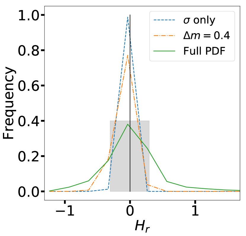
Figure 1: Comparison between three different Probability Distribution Functions for the $H_{r}$ of 1034 T-1. All distributions are centered at the median value of the magnitude obtained with the Full PDF. The blue dashed line considers only the errors in the magnitude, the orange dot-dashed line considers a single $\Delta m=0.4$, and the continuous green line considers all possible values of $\Delta m$ and the photometric errors (see text). The black vertical line represents the zero (i.e., the median of the Full PDF), while the shaded area covers the interval where the 68% of the solutions lie in the green curve.

In this case, $H_{r}$ is very precisely estimated (see Table 1). Nevertheless, the quoted uncertainty ($\sigma_{H_{r}}=0.04$ mag) does not reflect any possible effect of rotational variations in the magnitude, which will probably be larger than 0.04 based on its approximated diameter (between 3 and 6 km depending on its albedo), unless all observations were performed when the object was on a pole-on configuration. Nevertheless, we do not know this a priori, and it is unlikely that all observations were carried with such configuration.

3.1.2 Second test

The previous test did not include the effect of any possible rotational variation between different observations. This effect can be quite dramatic. According to the light-curve database (Warner et al., 2019) there are objects with $\Delta m=3.0$ mag, which may radically change the PCs if the effect is not taken into account. To test its effects, we ran a second test similar to the first, but in this case, instead of selecting $rand_{i}$ from a normal distribution, we selected it from a uniform distribution $\in[-\Delta m_{med}/2,\Delta m_{med}/2]$, where $\Delta m_{med}=0.4$ is the median $\Delta m$ from the whole small body population. The outcome of this test is also displayed in Fig. 1 but in orange dot-dashed line, labeled as $\Delta m=0.4$. In this case, the distribution of $H_{r}$ (called posterior distribution) is broader than in the previous test, $\sigma_{H_{r}}=0.14$ mag, which may appear as more realistic, but in this case, we are only considering one possible rotational state of the object, which may not be the correct one.

3.1.3 Including $\Delta m$ and $\sigma_{m}$

From the two previous tests, it is possible to see that including only the errors in the magnitudes ($\sigma_{m}$) provides a very precise value of $H$ (see also Table 1), but it does not represent the real spread of the data (please remember that we are dealing with sparse data taken at unknown rotational phases). If we only include the effect of $\Delta m$, the spread of the posterior distribution $H$ increases, providing less precision but possibly more accuracy, without significantly changing the mean (nor the median) values of $H$ (Table 1). Nevertheless, even if we chose a similar method as in Alvarez-Candal et al. (2019) where $\Delta m$ was chosen according to an estimate of $H$, this does not reflect the whole space of possible values that $\Delta m$ could take for an object with a given $H$. This is because different objects with similar $H$ may have different values of $\Delta m$. Therefore, we have adopted a new approach that includes the effect of the individual uncertainties in the magnitudes and also the whole space of possible values of $\Delta m$, i.e., it includes the values of $\Delta m$ for all objects with $H_{V}$ similar to the object of interest.

Table 1: Absolute magnitude estimates for asteroid 1034 T-1. The first column indicates the method, the second column the mean value, the third column shows the median value, and the fourth the standard deviation as a proxy for the width of the distributions

. [h] Method $\overline{H_{r}}$ $\tilde{H_{r}}$ $\sigma_{H_{r}}$ $\sigma$-only 14.95 14.92 0.04 $\Delta m=0.4$ 14.94 14.88 0.14 Full PDF 14.99 14.99 0.45

The method we devised includes the following steps (per object and per filter):
$1^{st}$ – using Eq. 1 we ran 10 000 different solutions following Test 1, i.e., using only $\sigma_{m}$, and applying it only to $g$ and $r$, therefore, we computed $H_{g}$ and $H_{r}$. Using the transformations in Table 1 of Jester et al. (2005) for all stars with $R-I<1.15$ we computed $H_{V}$, obtaining its posterior distribution. We normalized this distribution to obtain a probability distribution function (PDF) in 30 bins, i.e., $P(H_{V})=\{P_{j}(H_{V})\}$, $j$ is an integer $\in[1,30]$.
$2^{nd}$ – from the distribution of $\Delta m$ vs $H_{V}$ (Warner et al., 2019) we extracted all values $\Delta m$ in each bin $j$ in $P(H_{V})$ and finally we summed them using the values of $P(H_{V})$ as weights:

$$P_{A}^{i}(\Delta m)=\frac{\sum_{j}{P^{i}(\Delta m|P_{j}(H_{V}))\times P_{j}(H_{V})}}{\sum_{i}{\sum_{j}{P^{i}(\Delta m|P_{j}(H_{V}))\times P_{j}(H_{V})}}},$$ (2)

where $P_{A}(\Delta m)=\{P_{A}^{i}(\Delta m)\}$ is the PDF of $\Delta m$ for object $A$ in 150 bins of width 0.02 mag, to cover the whole range of reported $\Delta m\in[0.0,3.0]$. The denominator is a normalization factor. With this procedure, we created a PDF of possible values of $\Delta m$ that the object could have (see an example in Fig. 2, left panel).
$3^{rd}$ – to create the final PDF that will be used to estimate the final range of possible solutions of $H$ in all filters, we must also include the uncertainty in the measurement of $m$. In this case we construct for each object and measurement the distribution $P_{A}(m)$ as a normal distribution with $\sigma=\sigma_{m}$ centered at $m$. The final PDF is the convolution of $P_{A}(m)$ and Eq. 2:

$$P_{A}(m,\Delta m)=\big{(}P_{A}(m)*P_{A}(\Delta m)\big{)}.$$ (3)

Note that, in order to include realistic values of $\Delta m$ in $P_{A}(m)$, the distribution in Fig 2 (left) was mirrored along the y-axis and scaled by a factor 0.5 in the x-axis. This is done because an object with a given $\Delta m$ takes values of $m$ in the domain $[m-\Delta m/2,m+\Delta m/2]$ (see the final distribution in Fig. 2, right panel).

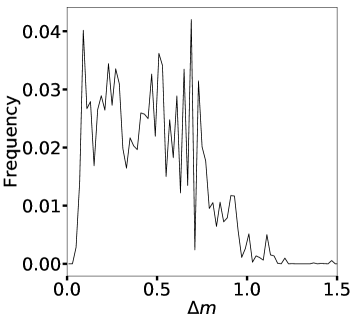
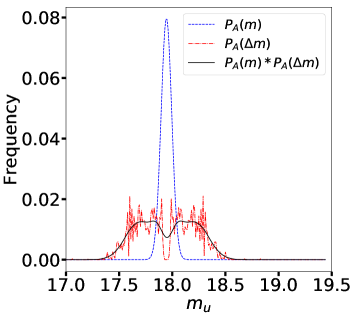
Figure 2: Left: Example of the Probability Distribution Function $P_{A}(\Delta m)$, cut at 1.5 in the x-axis for clarity, for asteroid 1034 T-1. Right: Examples of the PDFs used in this work.

Extracting 10 000 values randomly from $P_{A}(m,\Delta m)$ we ran the HG${}^{*}_{12}$ model obtaining the final values of $H$. The obvious consequence of our procedure is that the distribution of $H$ is very wide (see Fig. 1 in the continuous green line, labeled as Full PDF, and also see the values in Table 1). We remark that this is not related to the precision of $H$ but its accuracy.

Our final results are $H$ and $G$ distributions for each object and filter (stored in a compressed ASCII file). The files are available upon request. An example for the $H_{r}$ for the asteroid 1034 T-1 is shown in Fig. 1. We chose our representative value (see Table 2) as the median of the distribution and the uncertainties as to the values that enclose 68% of the solutions (seen in a continuous line and shaded region in the same figure).

Table 2: Sample of the catalog showing the ID in the first column, $H_{g}$ and its uncertainties in the second to fourth columns, the number of observations considered in the fifth and $G_{g}$ and uncertainties from column six to eight. The last two columns show the minimum $\alpha$ and its total span. The complete catalog is available in the folder provided in the text. The information is split into three different files, one with the $H$ and $G$, one with the IDs, and the last one with the angles. This was done so for simplicity. Flag -9999 indicates objects with less than 3 observations in a given filter, while flag -8888 indicates that not enough valid solutions were obtained (at least 100). The complete catalog is available at the CDS (https://cdsarc.u-strasbg.fr/) or upon request.

ID	$H_{g}$	$\sigma_{H_{g}}^{-}$	$\sigma_{H_{g}}^{+}$	N	$G_{g}$	$\sigma_{G_{g}}^{-}$	$\sigma_{G_{g}}^{+}$	$\alpha_{min}$ (deg)	$\Delta\alpha$ (deg)
1013 T-2	16.81	0.32	0.41	4	0.56	0.40	0.35	7.42	16.19
1034 T-1	15.75	0.22	0.27	4	0.44	0.36	0.31	1.63	22.44
1041 T-3	16.30.	0.38	0.44	3	0.60	0.45	0.34	0.12	8.36
1093 T-2	-9999	-9999	-9999	2	-9999	-9999	-9999	4.13	23.24
1132 T-1	-8888	-8888	-8888	8	-8888	-8888	-8888	9.17	20.86

4 Results and discussion

We computed $H$ in all filters available in the MOC (see numbers in Table 3) following the procedure outlined above. In addition, we computed $H_{V}$ again using $V$ obtained from $g$ and $r$ for each $\alpha$ where both magnitudes were available. Using $V$ and the corresponding $\alpha$, we processed the data the same way as all the rest. These computations have a multi-fold objective: First, to compare our procedure with previously published works. In particular with Oszkiewicz et al. (2011, O11 from now on), Vereš et al. (2015, V15), and Colazo et al. (2021, C21). Second, to check the validity of using the HG${}^{*}_{12}$ model, which is developed to obtain absolute magnitudes in the V filter. Third, for future studies that will include albedos in order to estimate diameters. We also include a comparison with Mahlke et al. (2021, M21) as other work with multi-wavelength PCs.

Table 3: Number of absolute magnitudes obtained

Magnitude	N	Concept	N
$H_{u}$	13 299	at least one valid $H$	14 801
$H_{g}$	14 081	with the 5 $H$ valid	12 252
$H_{r}$	14 543	in common with O11	3 879
$H_{i}$	14 485	in common with V15	8 050
$H_{z}$	14 104	in common with C21	521
$H_{V}$	14 440	in common with M21 (orange)	2 743
		in common with M21 (cyan)	1 316

In Fig. 3 we show an example of the PCs for asteroid 1034 T-1 in the five filters of the SLOAN system and also in the transformed V filter. The curves represent the data satisfactorily, making us confident of the procedure we followed (see also Sect. 4.7 below).

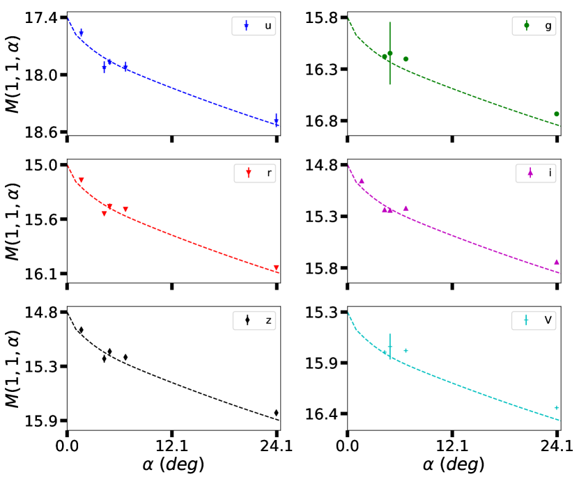
Figure 3: Phase curves in all filters for asteroid 1034 T-1. The phase function correspond to the representative values.

From the sample point of view, most objects have only three observations, although there are some with more than ten as well (Fig. 4, left panel), while the majority of objects are observed with $\alpha_{min}\sim 5$ degrees. Note that there are objects observed from near opposition up to $\alpha\sim 25$ degrees (Fig. 4, right panel), being most of them Main Belt asteroids.

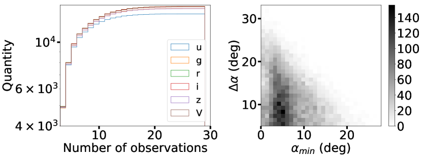
Figure 4: Left panel: cumulative distribution of number observations per filter for the objects in this work. Right panel: minimum $\alpha$ vs. span in $\alpha$ covered by the objects in this work.

The distributions of absolute magnitudes in all filters are displayed in Fig. 5.

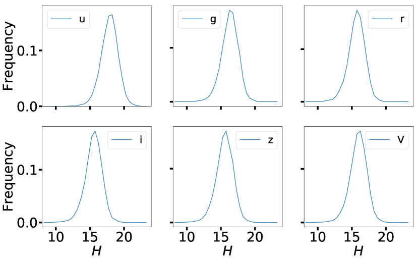
Figure 5: Frequency distribution of $H_{j}$ obtained in this work.

From the figure, it is clear that the $H_{u}$ distribution is fainter than the others by about two magnitudes, which is compatible, but still slightly larger, with the solar $(u-g)=1.43$. Overall, a systematic decrease in brightness towards u filter indicates mostly positive spectral slopes in the $H_{u}-H_{m}$ colors. The solar colors could explain part of this systematic, but not all.

4.1 HG₁G₂ vs. HG${}^{*}_{12}$

As described in Penttilä et al. (2016), the HG${}^{*}_{12}$ model is well suited for PCs with sparse coverage, which is the case of our work, with some limitations for some taxonomical classes (see Sect. 4.7). Nevertheless, recently, M21 showed that $H$ obtained from the HG${}^{*}_{12}$ model are systematically offset from $H$ obtained using the full HG₁G₂ model. Their results were obtained using ATLAS data on about 100 000 asteroids in two filters.

To check whether our $Hs$ are trustworthy, we ran the whole code using the full HG₁G₂ model and compared the absolute magnitudes obtained. The results for $g$ are shown in Fig. 6; in all other filters, the results are qualitatively and quantitatively similar (see Table 4). We chose a percent representation of the data in the histograms to remove the impact of the actual value of $H$ in the comparisons, for instance, a 0.5 mag difference at $H=10$ implies a 5 % difference, while at $H=20$ it implies a 2.5 %. For an object with $H_{g}=16$, the median value in Table 4 indicate a median difference of 0.05 magnitude, well below our median uncertainties. Therefore we conclude that $H$, as computed with the HG${}_{12}^{*}$ model, is well suited for our purposes. This does not preclude that, in the future, and if the data better cover the PCs, we adopt the HG₁G₂ model.

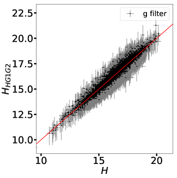
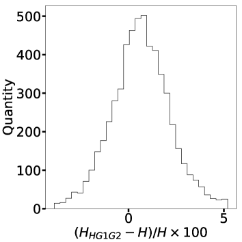
Figure 6: Left panel: Comparison between $H_{g}$ obtained by us using the HG${}_{12}^{*}$ (labeled $H$) and the magnitude obtained using the full HG₁G₂ models. The red line indicates the 1:1 relation. Right panel: Distribution of the percentual differences between the obtained $H$, the x-axis was cut for clarity.

Table 4: Comparison of absolute magnitudes. The first column shows the magnitude, the second (and fourth) the number of objects in common, the third (and fifth) the median difference, the maximum, minimum and standard deviation.

Magnitude	N	$(H_{HG1G2}-H)/H*100$ (%)	N	$(H_{no\,OE}-H)/H*100$ (%)
		[median, min, $\sigma$, max]		[median, min, $\sigma$, max]
$u$	5 455	-0.06, -23.7, 2.1, 9.7	3 242	0.05, -32.7, 3.4, 12.7
$g$	7 257	0.33, -24.7, 2.0, 11.5	3 515	0.16, -37.4, 2.8, 12.9
$r$	7 796	0.32, -26.5, 2.0, 10.8	3 644	0.13, -40.9, 2.9, 11.6
$i$	7 703	0.52, -28.0, 2.1, 11.3	3 615	0.07, -41.2, 3.0, 12.2
$z$	6 909	0.45, -27.8, 2.2, 11.8	3 526	0.04, -40.8, 3.3, 9.2
$V$	7 635	0.37, -25.8, 2.0, 12.6	3 611	0.12, -40.7, 2.9, 9.0

M21 argued that the HG${}_{12}^{*}$ was not precise enough because of a systematic difference in the absolute magnitudes obtained and also because the $G_{12}^{*}$ parameters they obtain tend to cluster towards 0 or 1 (see their Figs. 4 and 5). Nevertheless, we do not see the same trend. Our $G$-values have the shape of a wide bell. See, as an example, the comparison of $G_{cyan}$, $G_{orange}$, and our $G_{V}$ in Fig. 7.

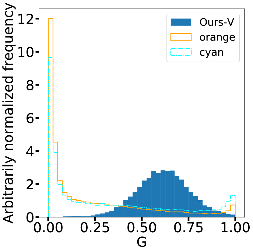
Figure 7: Comparison between $G$ values, in different filters, obtained in M21 for the ATLAS survey (cyan and orange histograms) and $G_{V}$ in the blue histogram.

4.2 Opposition effect impact on our estimations of $H$

As seen in Fig. 4 (right panel), many of the objects analyzed in this work have $\alpha_{min}>5$ degrees; therefore, their data do not cover the highly non-linear region of the opposition effect (OE). That may account for systematic differences between $H$ obtained using PCs with data in the OE region with respect to data that do not. To test if this could affect our results, we run the code, using the HG${}_{12}^{*}$ model but removing all data below 5 degrees. In this way, we can compare directly the same objects and check the impact of not covering the OE region. A comparison can be seen in Fig 8. Numerical relevant values are shown in Table 4. Note that we restrict the comparison to the objects that had data removed; if initially, they did not have any data below 5 degrees, they were left unchanged.

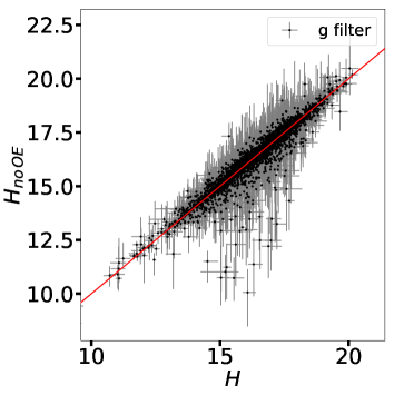
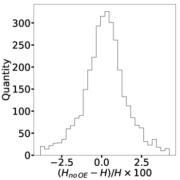
Figure 8: Left panel: Comparison between $H_{g}$ obtained by us (labeled $H$) and the magnitude obtained eliminating all data with $\alpha<5$ degrees. The red line indicates the 1:1 relation. Right panel: Distribution of the percentual differences between the obtained $H$. The x-axis was cut for clarity.

The median values are close to zero. For instance, for an object with $H_{g}=16$, the median impact will account for a difference of 0.03 mag, well within our median uncertainties. Nevertheless, it is possible to see some substantial discrepancies, especially some objects that come out as brighter when the low-phase angle data is removed. These $H$s correspond to objects with a low number of observations, as shown in Fig. 9. In the figure, the x-axis corresponds to the number of observations in the g filter before removal.

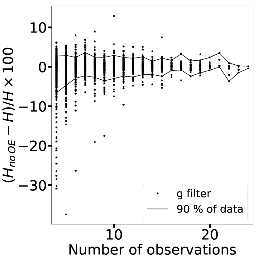
Figure 9: Number of observations per percentile difference. The continuous lines enclose the region where 90 % of the solutions lie.

The large differences seem to be related to significant uncertainties that arise when removing one or two points at low-phase angles from original data with four to ten input points. We do not detect any other strong systematic in our results. Therefore removing the OE region affects the uncertainty in the results when the original PC had few data points. However, we strongly remark that this does not happen for all objects. Therefore, we regard our results as trustworthy.

4.3 Comparison with other works

We compare our results with the four works mentioned above: O11, V15, C21, and M21. The former work presented over 400 000 PCs of objects using data compiled from the Minor Planets Center. Initially very heterogeneous in observatories, instruments, and filters, these data were carefully calibrated to a V filter magnitude to be analyzed. In V15 were presented almost a quarter of a million $H_{V}$ from the Pan-STARRS data release 1. The magnitudes were computed using Monte Carlo techniques to include effects of rotational variations and taxonomy heterogeneity. The data were magnitudes obtained in SLOAN-like filters that were transformed to $V$. With this comparison, we aim to check the quality of our results with a well-tested sample. In the case of C21, they used data from the Gaia DR2. In particular, we will compare with the sample of objects observed only with the Gaia G filter ($\gtrsim 14\,000$ objects), without transforming it to $V$. Due to the scanning law used by Gaia, these data were taken with $\alpha>10$ degrees. This comparison aims to see how our data compare with one of the largest databases of small bodies photometric measurements. Finally, M21 presented 127 012 PCs for 94 777 asteroids in a two-filter system: cyan and orange. The absolute magnitudes and phase coefficients were obtained using Bayesian inference and a Monte Carlo approach and reported as the mean values of the posterior distributions and the 95 % high-density interval, i.e., the interval where lie 95 % of the solutions.

The first three works used the HG₁₂ system as presented in Muinonen et al. (2010) and not the HG${}_{12}^{*}$ version presented in Penttilä et al. (2016) (O11 and V15 came out before it was published), while M21 did use the HG${}_{12}^{*}$. Keep in mind that $G_{12}$ and $G_{12}^{*}$ are not the same quantities. Due to this heterogeneity, we focus our comparison on the absolute magnitudes and not the phase coefficients, although, as shown below, we can draw useful information from the distribution of uncertainties of the different catalogs.

Figures 10 to 14 show the comparison of the $H$ values from all researches ($H_{V}$ from this work, O11, and V15, $H_{G}$ in C21, and $H_{cyan/orange}$ in M21). C21 reached a brighter population than the other four works (see the numerical comparison in Table 5). The difference cannot be explained only by the difference in the filters used: For an object with the color of the Sun $(V-R)=0.352$ (from Ramírez et al., 2012) and using the transformations from Gaia system to Johnson-Cousins we obtain $(G-V)=-0.13$. Interestingly, this result explains half the difference between our $H$ and C21’s (see Table 5). M21’s magnitudes are also brighter than our $H_{V}$, and these of O11 and V15, although not as much as C21. On the other hand, our distribution of $H_{V}$ is very similar, though slightly brighter but still within one standard deviation of the distributions ($\gtrsim 1$ mag), to O11’s and V15’s.

Table 5: Comparison between this work, O11, V15, C21, and M21.

	Median		Median (standard deviation)
$H_{V}$ (Ours)	16.0	$H_{V}$ (Ours) - $H_{V}$ (O11)	0.23 (0.27)
$H_{V}$ (O11)	16.0	$H_{V}$ (Ours) - $H_{V}$ (V15)	-0.13 (0.33)
$H_{V}$ (V15)	16.1	$H_{V}$ (Ours) - $H_{G}$ (C21)	0.26 (0.89)
$H_{G}$ (C21)	12.9	$H_{V}$ (Ours) - $H_{orange}$ (C21)	0.40 (0.28)
$H_{orange}$ (M21)	14.6	$H_{V}$ (Ours) - $H_{cyan}$ (C21)	0.06 (0.27)
$H_{orange}$ (M21)	14.4
	Median Uncertainty		Median Uncertainty
$H_{V}$ (Ours)	0.33	$G_{V}$ (Ours)	0.39
$H_{V}$ (O11)	0.07	$G_{12V}$ (O11)	0.33
$H_{V}$ (V15)	0.24	$G_{12V}$ (V15)	0.26
$H_{G}$ (C21)	0.98	$G_{12G}$ (C21)	0.55
$H_{orange}$ (M21)	0.01	$G^{*}_{12orange}$ (M21)	0.06
$H_{cyan}$ (M21)	0.02	$G^{*}_{12cyan}$ (M21)	0.08

We also compared the uncertainties in the five works. Note that we defined the uncertainties as to the interval edges where 68% of the solutions lie. This gives asymmetric quantities when referred to the median of the distribution. In order to compare our uncertainties, we chose as the metric the uncertainty defined as $\{[(\sigma_{H_{V}}^{+})^{2}+(\sigma_{H_{V}}^{-})^{2}]\times 0.5\}^{0.5}$. The uncertainties in O11 were treated similarly. In M21 are not reported uncertainties, but instead, magnitudes corresponding to the limits of the 95 % high-density interval. We will consider this interval as the formal uncertainty. It is clear from Fig. 10 that M21 and O11 have very precise values of $H_{V}$, with uncertainties lower than the other three. Most of M21’s uncertainties, in both filters, lie within the first bin in the figure that is the reason for the abrupt behavior of the curve. Meanwhile, C21 has a long tail of high-uncertainty $H$ and $G$. Our data seem to have larger uncertainties than O11, V15, and M21. However, they do not have the considerable uncertainties that appear for C21, especially in $G$. The long tail of highly uncertain values seen in C21 is possibly related to the fact that their data do not reach $\alpha<10$ degrees (see also Table 5). The authors complemented their PCs with ground-based $V$ magnitudes (previously transforming Gaia $G$ magnitude to $V$) to cover $\alpha<10$ degrees. Unfortunately, there are only six objects in common with our results, therefore precluding any reliable comparison.

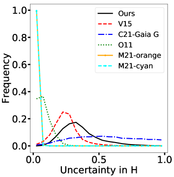
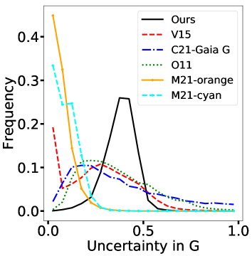
Figure 10: Comparison of the frequency distributions of the uncertainties in $H$ (left panel) and $G$ (right panel) between this work (black continuous line), O11 (green dotted line), V15 (red dashed line), $H_{G}$ of C21 (blue dot-dashed), $H_{cyan}$ (cyan dashed curve with big dots), and $H_{orange}$ (orange continuous line with big dots), the last two from M21. The x-axes were arbitrarily cut at 1 to exclude large values.

So far, we have compared the whole valid datasets (note that, for example, in V15’s online catalog, there are lines with negative uncertainties, which we do not consider valid). Now we compare the objects that are in common. First, we compare our results with O11, then with V15 and C21, and finally with M21 (significant numbers are already displayed in Table 5). As mentioned above, it is not possible to compare the values of $G$ because they were obtained using different definitions. Nevertheless, we can compare the absolute magnitudes obtained.

Our first comparison is with O11’s $H_{V}$ (Fig. 11). The red line over-plotted corresponds to a 1:1 correlation. The comparison is made over 3 879 objects in common $H_{V}\in(10,18)$. The agreement is good between both estimates of the absolute magnitudes, being ours fainter than O11’s with a median difference of 0.23 mag, while most objects have a difference in $H_{V}$ between 0 and 0.5 mag. We consider the agreement to be quite good.

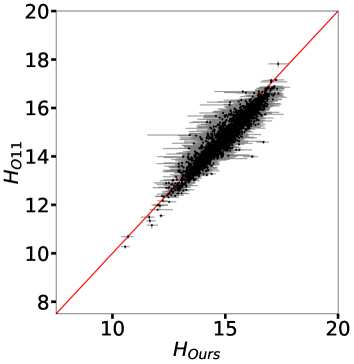
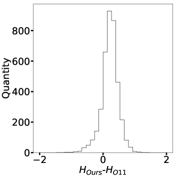
Figure 11: Left panel: Comparison between $H_{V}$ obtained by us and in O11. The red line indicates the 1:1 relation. Right panel: Distribution of the differences between the obtained $H$.

Figure 12 (left panel) shows the comparison between $H_{V}$ from this work and those published in V15. The figure shows that there is a very good agreement between both sets (8 050 objects in common), being our magnitudes slightly brighter than V15’s (median difference -0.13 mag), while most of the objects lie between a range of 1 mag centered in 0 (right panel of Fig. 12).

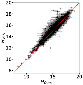
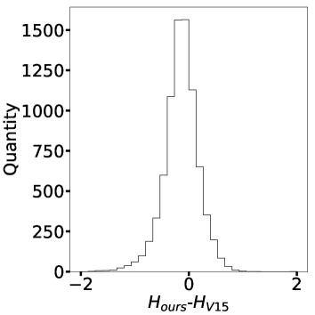
Figure 12: Left panel: Comparison between $H_{V}$ obtained by us and in V15. The red line indicates the 1:1 relation. Right panel: Distribution of the differences between the obtained $H$.

Next, we compare with a less dense database than the others, but with data that will probably become a benchmark of PCs studies. We compare with Gaia DR2 data as presented by Colazo et al. (2021) (Fig. 13). There are only 521 objects in common (some of them with non-valid results). Let us stress that their results were obtained using the G filter of Gaia, which is very broad when compared with the V filter. Overall, the data seems to follow the same trend, being C21’s magnitudes brighter than ours (median difference 0.26 mag), which makes sense considering the broader nature of the Gaia G filter. In this case, it is possible to see more spread in the difference of magnitudes, while most of the objects lie $H_{C21}-H_{ours}\in(-0.5,1.0)$.

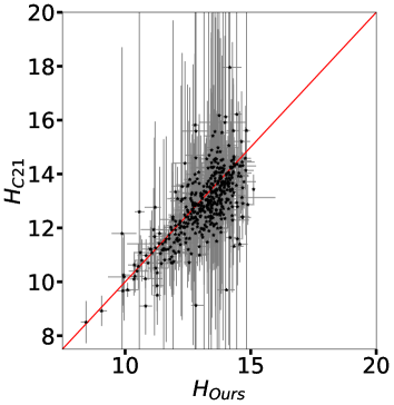
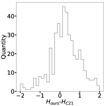
Figure 13: Left panel: Comparison between $H_{V}$ obtained by us and $H_{G}$ obtained by C21. The red line indicates the 1:1 relation. Right panel: Distribution of the differences between the obtained $H$.

Finally, we show the comparison with the ATLAS database (Mahlke et al., 2021). These data were obtained in two filters: cyan and orange, which are broader than the V filter. We have 1 316 objects in common with the cyan magnitudes and 2 743 with the orange magnitudes (Fig. 14). The comparison is quite good in both cases, especially with the cyan magnitudes (median difference 0.06), while our $H_{V}$ tends to be fainter than M21’s (median difference about 0.40). This may be because the cyan filter covers most of the V filter, while the orange filter only covers the reddest part of the V filter transmission curve.

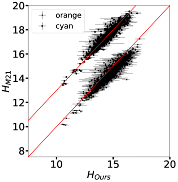
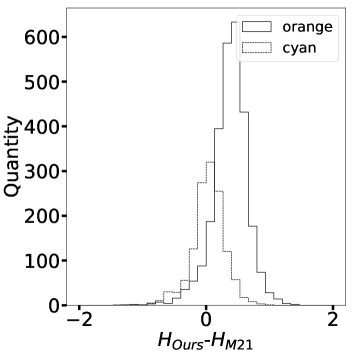
Figure 14: Left panel: Comparison between $H_{V}$ obtained by us and $Hs$ obtained by M21. The red line indicates the 1:1 relation. The comparison with the cyan magnitudes were shifted by 3 in the y-axis for clarity. Right panel: Distribution of the differences between the obtained $H$.

4.4 Zero phase angle colors

Following Ayala-Loera et al. (2018) we define the absolute colors as the difference in the absolute magnitudes in different filters. These colors are not affected by phase coloring and therefore represent a template to study these effects. The colors are shown as heat diagrams in Fig. 15. A quick comparison with Fig. 8 in Ivezić et al. (2001) shows that the space covered is similar (but logically lower in numbers).

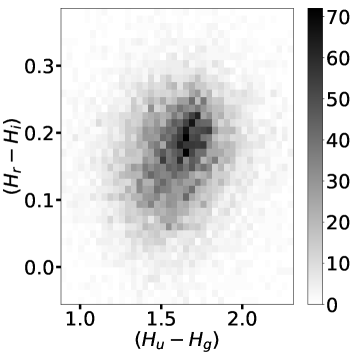
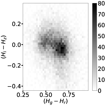
Figure 15: Absolute color - color diagrams. The axes were cut to exclude a few remaining outliers.

In this work, we do not attempt to study the possible taxonomical distribution of our objects (as done in Oszkiewicz et al. 2012), nor its distributions. These issues will be addressed in a future work. Nevertheless, it is clear, especially looking at the right panel of Fig. 15, that we do recover the large bimodal distribution of colors, historically representing the C and S type asteroids (see, for example, Hasselmann et al. 2015) while also seeing a tail of object going down to $(H_{g}-H_{r})\approx 0.7$ and $(H_{i}-H_{z})<0$ associated to V-type asteroids.

4.5 Absolute colors vs. average colors

One of our motivations is to produce a series of data that are not affected by phase coloring and can, therefore, be used with confidence to study, for example, the taxonomical distribution of objects in the main belt of asteroids. In Fig. 16 we show the weighted average of the colors per object compared with their respective absolute colors. These weighted colors were computed as the weighted average of the same data used to create the PCs. The weights are $1/\sigma_{m}^{2}$. The weighted standard deviation gives the error in each average color. Both sets of colors correlate (in all cases, the Spearman test produced $r_{s}\gtrsim 0.5$ and $P_{r_{s}}\approx 0$), but it is clear that there is not a 1 to 1 relation, reinforcing the idea that the average colors, although useful, do not necessarily represent the actual colors of the object and should be interpreted with great care.

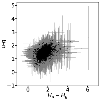
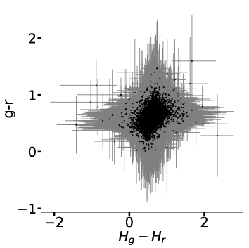
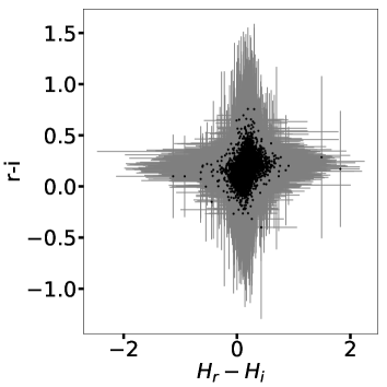
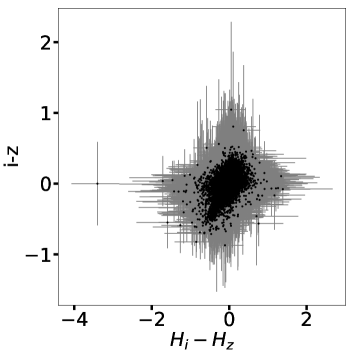
Figure 16: Absolute colors vs. average colors: Top left, $u-g$; top right, $g-r$; bottom left, $r-i$; bottom right, $i-z$. The typical (median) error bars are shown separately for clarity.

4.6 Absolute colors and $\Delta G$

We looked at the possible relationship between the absolute colors and the $G$ values we obtained. In Fig. 17 we show the absolute colors vs. the difference in $G$. There seem to be weak anticorrelations (see Table 6) between these quantities, possibly analogous to these found for TNOs (Ayala-Loera et al., 2018; Alvarez-Candal et al., 2019). In the latter work, we proposed it was related to a predominance of single-scattering at a low-phase angle, but the same cannot be said here because, first, $G$ is not the same as the phase coefficient $\beta$ obtained from a simple linear model, and second, the PCs in this work are mostly of asteroids obtained at a wide range of phase angles (see the right panel of Fig. 4).

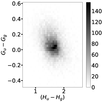
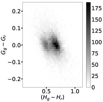
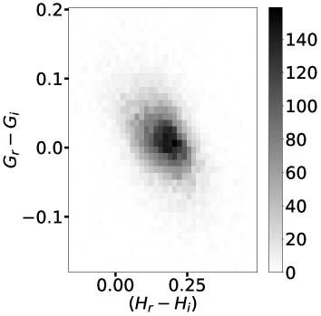
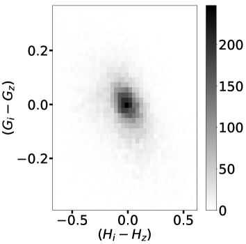
Figure 17: Absolute colors vs. the difference $G$ for pairs of filters: Top left, $u-g$; top right, $g-r$; bottom left, $r-i$; bottom right, $i-z$.

Table 6: Results from the Spearman rank-order correlation test.

Pair	$r_{s}$	$P_{r_{s}}$
$(H_{u}-H_{g})$ vs. $(G_{u}-G_{g})$	-0.27	0.0
$(H_{g}-H_{r})$ vs. $(G_{g}-G_{r})$	-0.38	0.0
$(H_{r}-H_{i})$ vs. $(G_{r}-G_{i})$	-0.45	0.0
$(H_{i}-H_{z})$ vs. $(G_{i}-G_{z})$	-0.37	0.0

Interestingly, in the $g-r$ space, there seem to be two parallel sequences. We do not have a clear explanation yet, but these overall behaviors could be due to some unexplored phenomenon happening at a low-phase angle.

4.7 Warnings and caveats

1. We explained in Sect. 3 that we have used the HG${}_{12}^{*}$ model presented by Penttilä et al. (2016). The $G_{12}^{*}$ parameter is not well suited for asteroids classed as E and D-type. Nevertheless, we decided to stick to our method because we do not know a priori the taxonomical classification of our objects. Besides, the results shown in Figs. 12 and 15 and Sects. 4.1 and 4.2 make us confident about our overall results. However, a revision will be done once we tackle the taxonomical classification of our objects.

2. The values we defined as representative of our quantities and uncertainty interval work well in most cases. Nevertheless, we identified a few cases where they were not the best representatives. In these cases, probably the mean, or mode, could work better. We stress that the method presented here is fully automatic and, due to the number of objects analyzed, it is impossible to perform checks for all objects. The readers have full access, upon request, to the distributions per object and filter of $H$ and $G$ and can therefore perform their analysis. Please note that there are solutions that do not have physical meaning in these distributions, for instance, values of $G<0$.

3. Our method intrinsically assumes that the variations in the brightness in all filters are due to rotational variation and that $P_{A}(\Delta m)$ is the same in all filters (i.e., due to form rather than different surface properties). We believe this is a reasonable trade-off between massive computation (and large numbers for statistics) and individual targeted studies when using integrated light from point sources, although detailed space missions observations show heterogeneity (e.g. DellaGiustina et al., 2020).

4. We did not apply any correction due to observations taken in different apparitions (changing aspect angle), which may be reflected in the PCs (see Fig. 10 in Mahlke et al. 2021 for an example). In the cases where this could have a significant effect, we expect it to be embedded in the posterior distributions of $H$ and $G$. We stress that we did not search for cases like this.

5. We still do not know the possible rotational phase at which each datum was obtained. This effect may be taken into account by multiplying each value of $\Delta m$ in $P^{i}(\Delta m|P_{j}(H_{V})$ by a random $\cos{\phi}$, where $\phi$ is the rotational phase that takes values in $[0,2\pi)$. Preliminary tests show that this approach needs better coverage of the PCs than that provided by the MOC to improve the results.

6. Figure 7 shows that our values of $G$ are distributed following bell-shape, centered more or less at values associated to C-type asteroids, see Fig. 2 in Penttilä et al. (2016), while it is expected that there should be many values at locations associated to S-type asteroids ($G\lesssim 0.2$). This is because our $G$ values are taken as the median of the posterior distributions determined in step 3 in Sect. 3.1.3. The median value is good for statistical analysis of large samples, but it may not be the best option when studying individual objects, as some distributions may appear flat, or bi- (or even multi-) modal.

5 Conclusions

We developed a method that includes Monte Carlo simulations and Bayesian inference to include the nominal errors in the magnitudes and the effects of rotational variations in the computation of phase curves with sparse data obtained by large photometric surveys. We applied the method to the SLOAN MOC and computed the phase curves of almost 15 000 objects obtaining $H$ and $G$ in the five filter system of the SLOAN survey. We also converted from $g$ and $r$ to $V$ to obtain $H_{V}$ and $G_{V}$.

We compared our results, especially $H_{V}$ and our uncertainties, with published catalogs to evaluate the performance of our method with respect to others. These tests proved satisfactory, granting confidence to the process. Although the method presented was developed with J-PAS and J-PLUS surveys in mind, it is flexible enough to be used with input magnitudes from other surveys, for instance, with data from the LSST, which will observe in a similar photometric system as the MOC and will add a filter in the near-infrared, the y filter (Ivezić et al., 2019). Therefore, we expect to apply the method to other catalogs, either multi-wavelength or not. Its effectiveness in near-infrared magnitudes, or other wavelengths, has yet to be checked.

Useful information can be extracted from the absolute magnitudes when translating them to reflectance values to construct photo-spectra, while the values of $G$ must be interpreted with care and should not be directly associated with taxonomical information. Finally, we would like to remark that the posterior distributions in $H$ and $G$ can be used when future data comes and other surveys for the same objects as priors to refine the computations and improve uncertainties.

Future work

The next steps, in no particular order, of this work, include:

• cross match with taxonomic information using the absolute colors.

• use the zero-phase colors to study color variations with $\alpha$.

• improve our algorithm, including possible effects of changing aspect angle using the shape models derived from Gaia DR3 photometry using inversion methods (Cellino et al., 2019).