Formation of ring-like structures in flared $\alpha$-discs with X-ray/FUV photoevaporation

Abstract

Protoplanetary disks are complex dynamical systems where several processes may lead to the formation of ring-like structures and planets. These discs are flared following a profile where the vertical scale height increases with radius. In this work, we investigate the role of this disc flaring geometry on the formation of rings and holes. We combine a flattening law change with X-ray and FUV photoevaporative winds. We have used a semi-analytical $1D$ viscous $\alpha$ approach, presenting the evolution of the disc mass and mass rate in a grid of representative systems. Our results show that changing the profile of the flared disc may favour the formation of ring-like features resembling those observed in real systems at the proper evolutionary times, with proper disc masses and accretion rate values. However, these features seem to be short-lived and further enhancements are still needed for better matching all the features seen in real systems.

1 Introduction

Planets form in accretion discs around Pre-Main Sequence stars, and understanding the evolution of these protoplanetary discs (PPDs) and the mechanisms and timescales by which these discs are eventually dispersed is a key issue in planet formation theories.

As the mass accretes onto star, the conservation of angular momentum implies that the disc spreads out, the accretion decreases with time and the radius increases with time. This transport can be explained in terms of internal viscous transport and magnetised winds, even when other possible mechanisms to consider may be planet formation, dust growth and encounters with other stars (Armitage and Hansen, 1999; Dullemond and Dominik, 2005).

Transition discs are PPDs characterised by a deficiency of disc material close to the star, exhibiting inner cavities or gaps in the distribution of the dust and/or gas (Andrews et al., 2011; Espaillat, 2014; Tazzari et al., 2017). Many of these inner cavities have sizes that can vary from sub-AU to many tens of AU, while there is still mass accretion onto the central star (Francis and van der Marel, 2020; Rometsch et al., 2020).

In addition to these internal cavities, ALMA data shows that the dust continuum emission of many, if not all bright and large, PPDs consists of rings and gaps, and one can find ring-like structures across the full ranges of spectral type and luminosity, up to a distance of around $100$au from their host star, with ages about $0.4-10$ Myr (Andrews et al., 2018; Long et al., 2018)).

An inside-out dispersal model produced by photoevaporation can naturally produce these internal cavities. When the thermal velocity exceeds the local escape velocity, the surface layer gets unbound and evaporates. Hence, the thermal winds remove mass regardless the angular momentum transport internal process, and the features seen in transition discs can be produced. The depletion can be produced by external radiation fields, when the disc is located in a populated and dense star forming region (Winter et al., 2018; Concha-Ramirez et al., 2019) or by internal radiation fields, generated by the host star itself (Alexander et al., 2006; Gorti and Hollenbach, 2009; Owen et al., 2012). Notably, the mass losses from both mechanisms are comparable, typically quoted as $10^{-8}$ $M_{\odot}/yr$ (Anderson et al., 2013).

These photoevaporative discs reproduce well some of the observed transition discs, mainly those with small cavities and low accretion rates, less than $10^{-8}$ $M_{\odot}/yr$. (Ercolano et al., 2018; Wolfer et al., 2019). However, they have problems to reproduce all observed discs (Owen et al., 2012; Marel et al., 2018). Therefore, many other mechanisms have been raised to explain the presence of ring-like fatures in young discs barely $1$ Myr old. Among these mechanisms, we can cite planets (Dong et al., 2015; Long et al., 2018; Huang et al., 2018), snow lines (Zhang and Jin, 2015), sintering (Okuzumi et al., 2016), instabilities (Takahashi and Inutsuka, 2016), resonances (Boley, 2017), dust pile-ups (Gonzalez et al., 2017), dead zones (Ruge et al., 2016), self-induced reconnection in magnetised discs wind systems (Suriano et al., 2018) or large scale vortices (Barge et al., 2017).

Obviously, PPDs are complex systems where different mechanisms leading to ring-like structures can be present at time, and one of these mechanisms might or not predominate. A common explanation for the observed ring-like features is the presence of planet-disc interactions. Therefore, these features are frequently considered tracers of new-born planets. However, it still remains how to match these widely found gaps at given distances with the small number of Jupiters mass planets around main sequence stars at those separations (Lodato et al., 2019).

The goal of our work is to analyse if simple photoevaporative viscous models can explain some of the observed ring-like features in PPDs while keeping the disc masses and accretion rates within the observed range of values. We will analyse the interplay of a variable flaring geometry and different photoevaporative winds in a variety of viscous $\alpha$-discs, exploring in a systematic way the impact of the different control parameters on the evolution and the formation of ring-like structures on those discs.

Viscous momentum transport is still of interest in disc modelling even when other transport alternatives are possible (Papaloizou, 2005; Heinemann and Papaloizou, 2009; Hartmann and Bae, 2018). The magnetorotational instability, or MRI (Balbus and Hawley, 1991), was for long time a leading candidate for turbulence and angular momentum transport. However, the MRI can be suppressed in non-ideal MHD (Riols and Lesur, 2018), and other mechanisms such as outflows, hydrodynamical processes and gravitational instability can be considered (Armitage, 2015; Kratter and Lodato, 2016). Moreover, magnetic fields can be of importance in momentum transport mechanisms and disc accretion may be primarily wind-driven with magnetised disc winds (Pudritz et al., 1991; Bai, 2016; Simon et al., 2017). Nevertheless, the presence of these magnetised winds does not exclude the presence of viscous transport.

The EUV flux was the first radiation field taken into consideration as a mechanism for the internal photoevaporation (Hollenbach, 1994). But EUV radiation leads to limited mass losses, while the FUV and X-rays radiation fields produce larger mass losses than EUV. Moreover, the X-ray winds are itself optically thick to EUV photons, and they prevent them from reaching the disc. Therefore, EUV is usually neglected when one considers the other two fields (Owen et al., 2012; Kimura et al., 2016).

The luminosities in FUV and X-ray wavelengths of young low-mass stars are significant and exceed by a factor $50$-$100$ the luminosities found in older stars like our Sun (Gómez de Castro and Marcos-Arenal, 2012). When modelling X-ray and FUV radiation, the hydrodynamic and thermal structure of the disc must be solved numerically, taking into account the irradiating spectrum, grain physics, chemical processes and cooling by atomic and molecular lines. This makes the modelling of each disc complex and computationally expensive. Hence, previous numerical studies dealing with these issues focused on analysing representative values of the host star mass and the viscosity (Anderson et al., 2013; Lodato et al., 2017). These studies are still being enhanced, by adding three-layers structures, metallicity dependences, improved modelling of gas temperatures and improved thermochemistry processes (Wang and Goodman, 2017; Nakatani et al., 2018; Picogna et al., 2019; Grassi et al., 2020).

Because of the complexity of the problem, we are going to take a semi-analytical $1D$ viscous $\alpha$-disc. Here, we can add a flaring profile that changes with time, and a photoevaporative term resulting from the combination of X-ray and Far-Ultraviolet (FUV) winds of different efficiencies.

A $1D$ model is by far much straightforward to implement, but it might be considered only valid while one does not include magnetic fields, envelopes or any other $2D$ or $3D$ structures. However, the complex hydrodynamics, chemical processes, and radiative processes can be incorporated in the form of function profiles resulting from numerical fits to the result of the more realistic simulations. In this way, semi-analytical $1D$ models are useful nowadays because their simplicity in interpreting the results allows to complement more complex hydrodynamical simulations.

We are going to numerically explore a grid of representative systems, analysing the evolution of the disc mass, the accretion rate and the creation of ring-like features as the stellar masses and initial disc mass are varied. Aiming to provide some insight on the role played by each parameter in better matching a numerical model with a real system, we will compare our results with an arbitrary sample of real systems in the Taurus star forming region, the same we selected in Vallejo and Gómez de Castro (2018). This will allow to probe the usefulness and limitations of this semi-analytical $1D$ approach.

The structure of the paper is as follows. The section 2 introduces the grid of $\alpha$-disc models. The section 3 shows the evolution of these models as the different control parameters, such as the viscosity, the flaring profile and the efficiency of a X-ray dominated wind, are varied. The section 4 presents the changes in the evolution of the discs when we combine both X-ray and FUV ionising fields. Section 5 is devoted to the analysis of the accretion rates in both cases. Finally, the last section summarises the results and makes some concluding remarks.

2 The numerical $\alpha$-discs

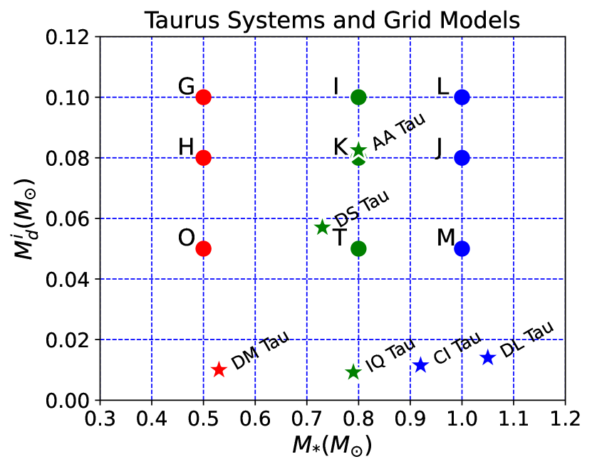
Figure 1: The selected grid of discs models in the $M_{*}-M_{d}^{i}$ plane. The initial disc masses $M_{d}^{i}$ decrease as the discs evolve. Hence, these initial points move downwards in the diagram, approaching to the Taurus systems from Table 1 that are also overlaid to the grid.

The Figure 1 shows the grid of systems that we will study. Every model of the grid is labeled with a given capital letter, keeping the same labels already used in Vallejo and Gómez de Castro (2018). This grid covers typical values for the host star mass $M_{*}$ and the initial mass of the disc $M_{d}^{i}$, meaning $M_{d}(0)$. This initial mass decreases with time as the disc is eroded, at a rate driven by the remaining control parameters. Conversely, the mass of the star $M_{*}$ can be considered to be constant as the accreted mass term does not add enough amount of mass to modify it.

As the initial disc mass of each numerical model decreases, their discs masses decrease, reaching the masses observed in real system at given ages. In this way, we can see how a real observed system can be best matched by a given model (or models) when these control parameters are varied in a given way. For doing so, we have overlaid to this figure the arbitrary selection of real discs listed in Table 1. These representative systems will be our reference sample. We have selected Taurus because it is one of the nearest and best-studied large star-forming regions. In addition, our work focuses on discs subject to radiation fields coming from the host star, and, in Taurus, the molecular cores can be considered isolated and the influence of outflows, jets, or gravitational effects is minimised (Hartmann, 2000). Other regions such as $\rho$-Oph or Orion are a good place for testing external photoevaporation models, but they are not the best environments for the analyses of disc sizes as diagnostic for isolated viscous evolution.

The Table 1 also includes data about the ring-like structures (rings and gaps) detected in those discs. A schematised view of the position of these structures can be seen in Figure 2. These data are listed just for reference. Some slight variations can be found along the literature because observational uncertainties, but we just aim to gain insights on the different mechanisms that may produce similar ring-like features at given ages on PPDs. For reference, the median age of Taurus stars is just a few Myr (Bertout et al., 2007), and a recent study (Luhman, 2018) shows that the older population of stars $>10$ Myr which was proposed to be associated with this region in other studies has no physical relationship with Taurus.

Table 1: Representative systems from the Taurus star forming region. The values for the star masses are those found in Simon et al. (2017). The values for disc mass, accretion rate and ages are those found in Jones et al. (2012). The X-ray Luminosity $L_{X}$ is computed from $M_{*}$ following Telleschi (2007). Additional viscosity data can be found in Vallejo and Gómez de Castro (2018).

Star	$M_{*}$	$M_{d}(t_{*})$	$M_{d}(t_{*})/M_{*}$	$L_{X}$	$log_{10}t_{*}$	$\dot{M}(t_{*})$	Rings-like
	($M_{\odot}$)	($M_{\odot}$)	(adim)	($erg\quad s^{-1}$)	($t_{*}$ yrs)	($M_{\odot}$ $yr^{-1}$)	brightness profile estructures
DL Tau	$1.05$	$0.0140$	$0.01$	$1.46\cdot 10^{30}$	$6.34$	$2.18\cdot 10^{-8}$	Gaps at $39$au, $66$au, $89$au. (Lodato et al., 2019; Long et al., 2020)
CI Tau	$0.92$	$0.0115$	$0.01$	$1.17\cdot 10^{30}$	$6.23$	$1.12\cdot 10^{-8}$	Gaps at $14$au, $48$au, $118$au. (Long et al., 2018; Lodato et al., 2019)
AA Tau	$0.80$	$0.0825$	$0.10$	$9.23\cdot 10^{29}$	$6.38$	$2.75\cdot 10^{-9}$	Cavity up to $28$au, gaps at $72$au, $115$au. (Marel et al., 2018)
IQ Tau	$0.79$	$0.0092$	$0.01$	$9.03\cdot 10^{29}$	$6.08$	$5.75\cdot 10^{-9}$	Gap at $41$au. (Long et al., 2018; Lodato et al., 2019)
DS Tau	$0.73$	$0.0570$	$0.08$	$7.90\cdot 10^{29}$	$7.23$	$1.00\cdot 10^{-8}$	Gap at $33$au. (Lodato et al., 2019; Long et al., 2020)
DM Tau	$0.53$	$0.0100$	$0.02$	$4.58\cdot 10^{29}$	$6.56$	$1.02\cdot 10^{-8}$	Cavity up to $16$, gap at $70$au. (Marel et al., 2018)

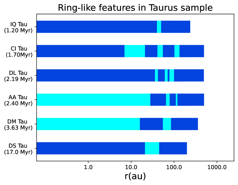
Figure 2: A schematised view of the position of the inner cavities and gaps of different widths that are observed in the Taurus reference sample (there is no detailed indication of the real density gradients). The discs are plotted as dark blue, and the cavities and gaps in cyan. For reference, ALMA spatial resolution in Band 6 is around $16$au at Taurus distance. See references given in Table 1 for details.

The calculation of the mass accreted by every host star of the grid can be done through the analysis of the evolution in time of the surface mass density $\Sigma(r,t)$ using the basic laws of mass and momentum conservation,

$$\frac{\partial\Sigma}{\partial t}=\frac{3}{r}\frac{\partial}{\partial r}[r^{1/2}\frac{\partial}{\partial r}(\nu\Sigma r^{1/2})]-\dot{\Sigma}_{w},$$ (1)

where $\dot{\Sigma}_{w}$ denotes the mass loss by a given photoevaporative wind, functionally equivalent to have a sink in this diffusion equation.

The viscous evolution of the disc is computed using a first-order explicit FTCS scheme. The computational mesh covers uniformly from $0.0025$ au to $2500$ au using the scaled variable $x$, where $r=x^{2}/4$. Zero-torque boundary conditions are applied in the inner and outer boundaries, meaning $\Sigma=0.0$ at both edges of the mesh. When solving Eq. 1, we use an initial profile $\Sigma(r,0)$ that follows the self-similar solution firstly used in Lynden-Bell and Pringle (1974).

The kinematic viscosity $\nu(r)$ is the coefficient that regulates the diffusion. When considering that the disc surface density follows a $r^{-\gamma}$ dependency, this kinematic viscosity can be modeled by,

$$\nu(r)=\nu_{1}(\frac{r}{R_{1}})^{\gamma}.$$ (2)

Different $\gamma$ values can be found in the literature. Some references use $\gamma=3/2$ (Lodato et al., 2017), but it is more frequent to use a linear dependency with radius, $\gamma=1$ (Clarke et al., 2001; Alexander et al., 2006; Rosotti et al., 2017). Therefore, we have selected this value for comparison purposes.

As a consequence of above, $R_{1}$ is the scale radius at which the viscosity has the value $\nu_{1}$. This $\nu_{1}$ just depends on the initial mass of the disc $M_{d}^{i}=M_{d}(0)$ and the selection of the initial accretion rate $\dot{M_{0}}$,

$$\dot{M_{0}}=\frac{3M_{d}(0)\nu_{1}}{2{R_{1}}^{2}}.$$ (3)

Once we have fixed the initial profile $\Sigma(r,0)$ and the functional form of Eq. 2, one can obtain $\nu_{1}$ from Eq. 3 and compute the viscous evolution as per Eq. 1. However, the initial value for the accretion rate $\dot{M_{0}}$ is not a good control parameter of the model because it is not an observable quantity. By other hand, the Shakura prescription, or $\alpha$-disc prescription, allow us to select the $\nu_{1}$ coefficient without presuming $\dot{M_{0}}$.

This parametrisation was firstly used in Shakura and Sundayev (1973) and later refined in Shakura and Sundayev (1976). It hides the details of the specific viscous transport mechanism while reflecting the impact of the transport in the disc evolution. Therefore, as this parametrisation simplifies the implementation of the viscosity in numerical models, it has been widely used for many years and it is still in common use today (Kimura et al., 2016; Lodato et al., 2017; Ercolano et al., 2017).

This model relies on an optically thick accretion disc and a turbulent fluid described by a viscous stress tensor, with this stress tensor being proportional to the total pressure. When the eddy size (mean free-path) is less than the disc height and the turbulent velocity smaller than the sound speed $c_{s}$, one can write the viscous profile as, $\nu(r)=\alpha c_{s}H(r)$, with $H(r)$ the scale height profile that models the disc thickness, presuming $H(r)<<r$ for a thin disc.

Considering hydrostatic equilibrium perpendicular to the disc plane and a simple relationship between the disc and surface temperatures, the sound speed can be written as $c_{s}=H(r)\Omega$, with $\Omega$ is the circular keplerian velocity (Jones et al., 2012). Hence, the $\nu$ viscosity at a given distance $r$ depends on rotation, with a linear dependency on the mass of the star $M_{*}$ and on the flaring of the disc,

$$\nu(r)=\alpha\frac{c_{s}^{2}}{\Omega}=\alpha\Omega H^{2}(r).$$ (4)

Figure 3: Different profiles for the considered flared discs. The parameters of the power law define the scale height $H(r)$ of the disc. The P5 profile means $\upkappa=0.05$, the P3 profile means $\upkappa=0.033$, the P2 profile means $\upkappa=0.02$, all using $h=1.25$. Hence, when using progressive flattenings, the label P52 means a profile changing from P5 to P2.

Therefore, the flaring profile is a key parameter that defines the $c_{s}$ profile, and, in turn, the temperature profile of the disc. The scale height $H(r)$ depends on the competition between thermal pressure and gravity. That is, between the temperature and surface density profile. And the temperature depends on the amount of stellar radiation impacting the disk, which also rests on its geometry again. By solving these coupled equations, Chiang and Goldreich (1997) found the scale height $H(r)$ can follow an approximate power law dependence,

$$H(r)=\upkappa\ r^{h},$$ (5)

with $h\sim 1.3-1.5$. However, fully-flared models based on a two-layer dust model do not properly reproduce the SED in the far-IR and a flattened disc flaring is required, typically by a factor $3$ (Tazzari et al., 2017). This flattened profile is then similar to those that use $h=5/4$ (Alexander et al., 2006; Owen et al., 2012; Rosotti et al., 2017) . This fullfils the condition for a geometrically thin disk and lead to a viscosity through Eq. 2 that scales linearly with radius (Hartmann et al., 1998; Alexander, 2007). Hence, we have used this value of $h$ as baseline profile. The Figure 3 shows these different flaring profiles for reference.

Even when it is customary to keep constant the flaring profile of the disc, it seems reasonable to consider that this flaring may change with time, with a progressive flattening of the disc as the age increases. This flattening can be due due to settling of dust grains toward the midplane (DAlessio et al., 1999; Chiang et al., 2001), and to occur very early in the evolution of a disc (Dullemond and Dominik, 2004). Obviously, discs with cavities are very diverse, not forming a single population of objects, and they could present very different dust growth and sedimentation (dust settling) laws (Williams and Cieza, 2011). Finally, the flaring geometry of the disc may differ when one considers if the photoevaporation is dominated or not by the X-ray (Owen et al., 2012). Therefore, we will include in our simulations a changing profile for the flared disc, by decreasing the $\upkappa$ parameter in Equation 5 at given times (see Section 3.2).

3 Photoevaporation from X-ray radiation dominated winds

The selection of the photoevaporation mechanism providing the mass sink term ${\dot{\Sigma}}_{wind}$ in Eq. 1 has important implications for the evolution of the discs. The models from Owen et al. (2012) suggested that the X-ray component dominates the photoevaporative mass-loss rates from the inner disc unless one may have high FUV-to-X-ray luminosity ratios ($L_{FUV}/L_{X}>100$), even when there is not a clear consensus about how X-ray and FUV (and even EUV) must be put together (Armitage, 2015). Because we aim to systematically analyse the role of every control parameter, our work starts with simulations based on winds presumed to be mainly driven by X-ray radiation.

In general, one can consider three sources for the X-rays: emission coming from the disc host star, emission coming from jets shocks (Ustamujic et al., 2016), and external emission in clusters (Adams et al., 2012). Here, we will focus on the internal radiation field coming from the host star. This X-ray heating rely in X-ray photons in the $0.1-10$ KeV range that can tear off the electrons from the internal shells of metals. These electrons produce further ionisations until the energy is thermalised. Higher energies photons can penetrate further, but do no provide significant heating (Owen et al., 2012).

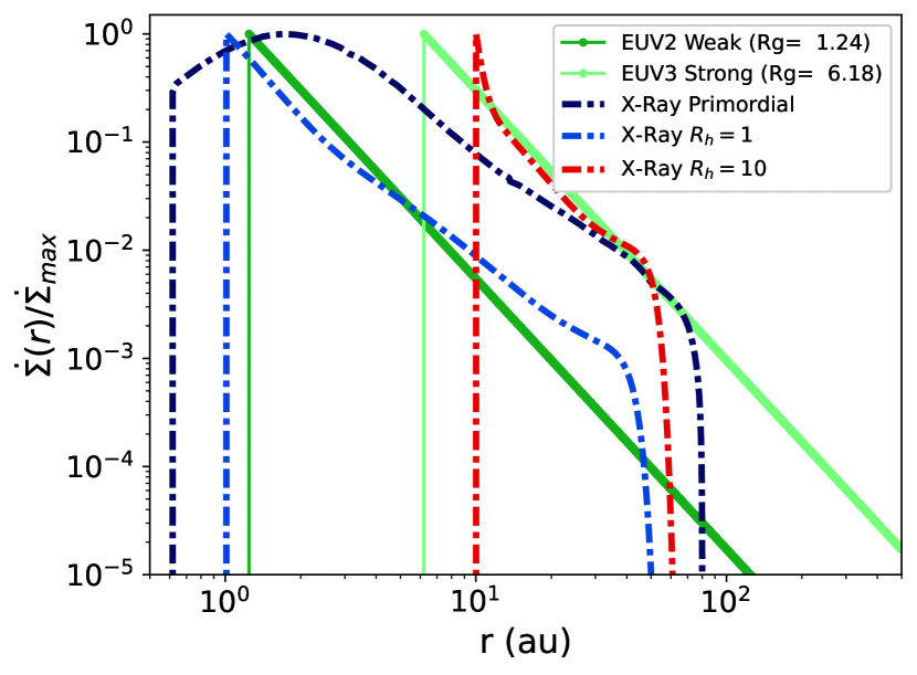
Figure 4: Photoevaporative wind mass losses for diferent X-ray cases and $L_{x}=1\cdot 10^{30}$ ($ergs$ $s^{-1}$). For comparison, one strong and one weak EUV wind mass profile are also plotted. The integrated mass rates along all radii have been set to unity and the resulting profiles have been divided by their maximun in order to compare the different shapes.

This heating is not straightforward to model because the hydrodynamic and thermal structure of the disc must be solved numerically taking into account the irradiating spectrum, grain physics, chemical processes and cooling by atomic and molecular lines. As we want to add these winds in our $1D$ semi-analytical model, we have used the same approach taken by Rosotti et al. (2013), Ercolano et al. (2017) and Kimura et al. (2016). Hence, we have used a photoevaporative X-wind mass sink term $\dot{\Sigma}_{wind}$ resulting from the numerical fit to the results of the simulations done by Owen et al. (2012).

This X-ray wind model has two different wind profiles, that are activated by the presence or not of a hole in the disc. The Figure 4 shows the photoevaporative wind mass losses $\dot{\Sigma}$ corresponding to each phase. The primordial phase profile corresponds to the initial stage that lasts until the wind eroding the disc opens a cavity on it. Then, the second stage begins, that lasts while this gap gets wider, as the inner edge of the outer disc is exposed directly to stellar irradiation. The figure also shows the second stage profiles corresponding to different sizes of this hole. This phase ends when the disc can be considered almost fully depleted as the floor density has been reached at all radii.

Just for reference, the Figure 4 also shows EUV winds: one weak EUV wind (labeled EUV2) and one strong EUV wind (labeled EUV3), as described in Vallejo and Gómez de Castro (2018). Meanwhile the EUV winds have more localised wind losses, and the disc is hardly depleted at large radii, the X-ray winds are stronger, with much shallower profiles and significant contributions at large distances.

One key parameter of this X-ray model is the computation of the instant when it switches from the primordial phase to the second phase. This can be done by monitoring the $\Sigma(r,t)$ at every $t$ in two different inner selected locations, $0.1$ au and $1.0$ au (Ercolano and Rosotti, 2015). The switch will take place when $\Sigma<10^{-5}gcm^{-2}$. As alternative, one can compute the column density $N_{H}$ at the inner edge of outer disc, and the switch will starts when $N_{H}<10^{22}$ (Ercolano et al., 2017; Kimura et al., 2016). Both approaches lead to similar results, and, for simplicity, we have selected the first option.

The expressions of the total integrated mass loss rate due to the X-ray wind are detailed in Owen et al. (2012), and they depend on the stellar mass $M_{*}$ and X-ray luminosity $L_{X}$. For $M_{*}=1$ $M_{\odot}$ and $L_{X}=10^{30}$ $ergs\quad s^{-1}$, the total integrated mass loss rate in the primordial phase is $\dot{M}_{X}=6.25\cdot 10^{-9}$ $M_{\odot}yr^{-1}$, meanwhile the total integrated mass loss rate in the second phase is $\dot{M}_{X}=4.8\cdot 10^{-9}$ $M_{\odot}yr^{-1}$. We will take these values as the baseline option for defining our fiducial X-ray wind.

3.1 Viscosity and timescales

The $\alpha$ parameter was initially introduced as a convenient scaling factor of the friction between adjacent rings. Later on, it turned into a standard dimensionless measure of viscosity, as a convenient way to hide the real viscosity mechanism. This dimensionless constant can take values between $0$ (no accretion) and close to one, presuming a subsonic regime for the turbulence. A recent discussion of the $\alpha$ parametrisation in other regimes can be seen in Martin et al. (2019).

The $\alpha$ prescription can be seen as mere re-parametrisation of the viscosity. But, one can also extend this approach, and to use a unique $\alpha$ value for modelling the viscosity of the whole disc. The variety of values for $\alpha$ then reflects the different effectiveness of the hidden viscosity processes found in different discs. Indeed, this effectiveness can take different values within the same disc at different locations (Bai, 2016). These issues may explain the variety of values returned from observations, sometimes being as high as $0.2-0.3$ in fully ionised discs, and sometimes being much less than that, lowering up to values $<0.01$ or even $0.001$ for not fully ionised discs (Martin et al., 2019).

Therefore, $\alpha$ is a main parameter controlling the disc evolution that can not be set arbitrarily. The observed disc masses and accretion rates in star forming regions such as Taurus, Chamaeleon I or Lupus, put constraints on the amount of viscosity to consider, see Martin et al. (2019) and references therein. However, there is no general consensus in the most suitable value for $\alpha$ even in the simplest scenario, when one neglects that the viscosity can evolve with time. Different $\alpha$ values may mean different metallicity values for the disc (Ercolano et al., 2018), and one can find a variety of values. The $\alpha=0.01$ was used in early studies because a viscosity sourced to MRI seemed to lead to this value (Hawley and Balbus, 1995), and also because it provides evolutionary timescales in line with known properties of discs (Hartmann et al., 1998). Later on, a wider rage of values was in used, with values in the literature spanning typically from $0.1$ to $0.001$ (Andrews et al., 2009; Gorti and Hollenbach, 2009; Jones et al., 2012). Finally, lower values like $10^{-4}$ are nowadays also found (Anderson et al., 2013; Ercolano et al., 2017), and our previous work with EUV winds points to these small viscosity values (Vallejo and Gómez de Castro, 2018).

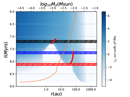
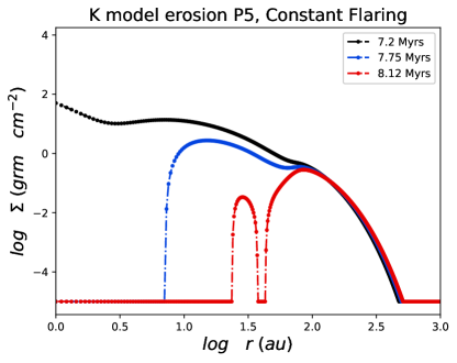
Figure 5: (Left panel) Density diagram showing the evolution of model $K$ under photoevaporation produced by X-ray dominated heating and a viscosity value of $\alpha=10^{-4}$, with a constant flaring profile $P5$. Earlier times are at the top of the figure, and the $y$-axis shows the time evolution of the surface density from top to down. The lighter the colour, the lower the density, with white colour indicating that the density floor level has been reached. The red dots indicate the local minima in the density profile. The upper horizontal axis shows the evolution with time of the disc mass as an orange curve. The black, blue and red horizontal patterns mark the times corresponding to the three density profiles on the right panel. (Right panel) Density profiles at three given times produced when slicing the density diagram. The initial dent can grow until it produces an internal cavity. If an additional dent in the density is produced, further gaps and outer ring-like features can be observed.

Hence, as starting point one can take the X-ray wind mass losses described in the previous section, a viscosity value of $\alpha=10^{-4}$, and a flared profile with a constant value $\upkappa=0.033$ (the P3 profile).

The wind flow first produces a dent in the density profile. This dent can will typically grow with time, becoming deeper and deeper until a gap in the density profile is produced. As the inner disc density decreases, it eventually reaches the floor level and an internal cavity is created.

The creation of this internal cavity flags the start of the second phase, when there is a direct flux wind coming from the host star. The wind profile in this second phase also has a peak at given location that moves farther away as the time goes, and will erode the outer portions of the disc. The larger the mass of the disc, the longer it takes to disappear. Conversely, the larger the stellar mass, the stronger the wind and the shorter the disc lifetime. However, the internal cavity typically seems to develop at around $10$Myrs, and the synthetic disc lifetimes can reach up to $20$Myrs for the largest initial discs and smallest host stellar masses.

One can make these lifetimes shorter by increasing the initial flaring, considering a flared profile with a constant value $\upkappa=0.05$. The left panel of Figure 5 corresponds to the evolution of the surface density $\Sigma(r,t)$ with time of the central model of the grid, the $K$ model, using the fiducial X-ray wind mass losses, a viscosity value of $\alpha=10^{-4}$, and the P5 profile. The bottom horizontal axis scale provides the density at given radii. The lighter the colour, the lower the density, with white colour indicating that the density floor level has been reached. These diagrams also provide information about when a dent in the density profile is produced, if the erosion is slow enough. These dents might eventually produce further gaps and outer ring-like features. The red dots indicate the dents as local minima in the density profiles. The right panel shows how slicing these diagrams at given times one can visualise these features in the density profiles.

Earlier times are at the top of the figure, and the $y$-axis shows the time evolution of the surface density from top to down. The internal gap begins to develop around $7$Myrs and the disc is completely eroded around $9$Myrs. In terms of temperature, the larger the $\upkappa$, the higher the temperature at a given radius. Hence, one gets a faster eroding in this case, and a shorter lifetime. As summary, the cavities seen in these simulations are very short lived, lasting just a few Myrs but for the smallest stellar masses and largest initial disc masses.

This Figure 5 also shows the evolution with time of the disc mass as an orange curve. The upper horizontal axis shows how fast the disc mass decreases with time.

Simulations using a higher viscosity value, $\alpha=0.001$, lead to the surface density to decrease faster. The synthetic models produce inner cavities, but have difficulties on creating ring-like structures at any age, unless we use very flattened discs. This is because the peak belonging to the wind front moves fast inside out, quickly eroding the external disc.

Dents and ring-like features can be also formed, but they are short-lived and created at very late times. Therefore, these simple photoevaporative models with constant flaring profiles can explain the generation of inner cavities and some ring-like features, but in a limited way. They do not fully account for creating the observed structures in transition disks of ages of Myr or less. Moreover, the internal cavities are only formed when the disc masses are much lower than the observed values, as reflected by the orange curves in the plots.

Hence, the age of the disc when the cavities and ring-like features appear is a key issue. One might consider that some of the parameters of the Taurus sample may be subject to observational uncertainties, mainly the ages. One may also take into account that the generation of a dent is not always followed by the creation of a gap in our models. However, the possibility of creating dents with this simple approach is important because once the dents are present, gas removal processes may trigger collective mechanisms for planetesimal formation such as the streaming instability or some increases in the dust-to-gas ratio, that may act as dust traps (Ercolano et al., 2017). Hence, in the following sections we will explore how to produce earlier in time these dents, keeping at the same time the proper disc mass.

3.2 The impact of a progressive flattening in the profile of flared discs

Discs are flared, as seen by spatially-resolved mid-IR imaging in nearby PPDs (Doucet et al., 2007; Maaskant et al., 2013). In these discs, the outer parts of the disc intercepts more radiation from the central star. Moreover, according to Equation 4, the selection of the flaring profile directly impacts the viscosity, thus the evolution of the disc. We want to analyse the impact of a changing profile of the flared disc as the disc evolves, with a progressive flattening of the disc as the age increases and the dust may settle at different rates. Hence, this section aims to analyse the role that these changes may have in the generation of ring-like features at outer radii.

We will model a decreasing flattening of the disc by decreasing the $\upkappa$ parameter in Equation 5. A decrease in the flaring of the disc means a decrease in the temperature profile. Hence, the accretion rate is made stronger, and one gets a faster starvation of the disc and the ring-like features might appear before.

As a first approach, we can take a model where the disc starts with a given flaring profile, keeping $\upkappa$ constant during the primordial phase. When the direct-flux phase begins, let us say, at $t_{direct}$, the disc is flattened by lowering the $\upkappa$ value. This new value remains fixed for the whole remaining disc lifetime.

This one step piecewise flattening is a very rough modelling of the expected continuous flattening to happen in real systems. Hence, the baseline for our synthetic models will consider a second run for each system. This second run is based on a $P52$ profile. This means that we start with an initial flaring value of $\upkappa=0.05$ that gradually decreases up to $\upkappa=0.02$ in five steps. The center point with the fiducial value $\upkappa=0.03$ is set at time $t_{direct}$, when the direct flux started in the first simulation run. Of course, one should note that the direct phase can start in the second run at a different time with respect the first simulation, because we have obviously changed the flaring profile of the disc.

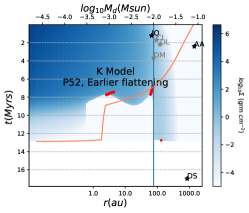
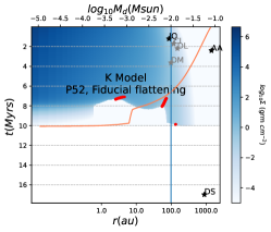
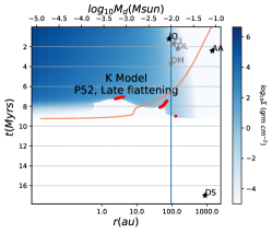
Figure 6: Density diagrams showing the impact of an earlier or late flattening process. They show the evolution of the central model of the grid (model $K$) under photoevaporation produced by X-ray dominated heating and a viscosity value of $\alpha=10^{-4}$, subject to a progressive $P52$ flattening of the disc. The center column is the fiducial flattening, that sets the value $\upkappa=0.033$ at $t_{direct}$ time (see text for details). The earlier the time when the progressive flattening starts, the longer the cavity lasts and the longer is the phase when ring-like features can exist.

The Figure 6 shows the impact of this progressive flattening in the evolution of the the central model of the grid (model $K$). The center column is the fiducial flattening, that sets the value $\upkappa=0.033$ at $t_{direct}$ time. As visual reference, the blue vertical line marks an arbitrary value of $0.01M_{\odot}$, that indicates when disc mass is very small.

One can consider that the actual flattening may start earlier or later than $t_{direct}$. Hence, this figure also shows the results when we move forward and backwards the time when flattening steps take place. The earlier the time when the progressive flattening starts, the longer the cavity lasts and the longer is the phase when ring-like features can exist. The lifetime of the disc seems to grow, as reflected by the orange curve. Conversely, when the flattening takes place later, it seems that the lifetimes are similar or slightly shorter.

When one compares these diagrams with those resulting from a constant flaring profile, one can see that internal eroding phase takes slightly longer. The orange curve shows that the disc mass will slow down in this phase. This allows the wind to slowly erode the outer parts of the disc before starting the direct phase, which can ease the creation of a third dent in the outer part of the disc.

$\xrightarrow{\makebox[170.71652pt]{$M_{d}$}}$
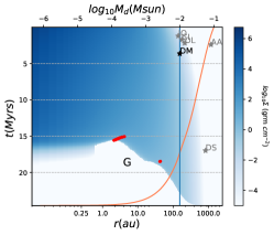
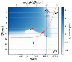
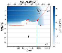
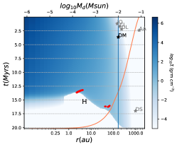
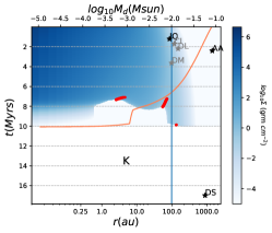
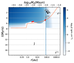
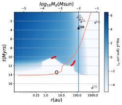
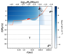
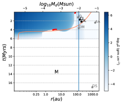
	$\xrightarrow{\makebox[170.71652pt]{$M_{*}$}}$

Figure 7: Evolution of the grid of models for a fiducial photoevaporation controlled by X-ray heating, $e_{x}=1.0$, a viscosity value of $\alpha=10^{-4}$ and a progressively flattened flaring profile $P52$. The surface density in blue gets lighter as the disc is eroded. The red points indicate local minima in the density profiles. The second dent can be carved at the same time or even at earlier times than the the inner dent. These two dents can produce ring-like features when exist at the same time. Sometimes, these two dents can be accompanied by a third outer dent. The Taurus discs are also plotted for reference. They appear in black when their stellar masses are similar to the mass of the analysed synthetic model. Otherwise, they appear in grey.

The Figure 7 shows the density diagrams corresponding to the evolution of the grid of models for a fiducial photoevaporation controlled by X-ray heating, a viscosity value of $\alpha=10^{-4}$ and this progressively flattened flaring profile $P52$. Because the time when the direct flux stage gets active is different in each model, the time when the flattening occurs is also different in each case.

The larger the stellar mass, the faster the creation of the inner cavity, and faster the decrease of the disc mass. Changes in the flaring profile means changes in the eroding rate. As a consequece, the systems with smaller host stellar masses and largest initial disc masses ($G$ and $H$) present somehow long-lived cavities, while the remaining systems show very short cavity lifetimes.

The red points indicating local minima (dents) show that as the stellar masses and initial disc masses increase, the second dents appear earlier. These dents (sometimes eventually converted into gaps) can produce ring-like features when exist at the same time that the first dent. Moreover, an additional third dent can be found in the systems with large enough disc masses ($K$,$I$ and $L$).

Following our simulations, the first close-to-star and the second external dents are not created at the same time. First, the inner dents are created. Then, a few Myr later, the outer structures appear. Notably, the second dent can be produced earlier than the first one when the initial disc mass is small enough, as best seen in models $T$ and $M$.

These dents may or not convert into gaps and lead to true rings. The dents sometimes do not evolve into real gaps, because the disc in the surroundings reaches the floor density before the dent fully develops. However, we will still refer to them as ring-like features, because such dents may be considered seeds for true rings. As we are dealing with very simple models, one can consider that such dents, linked to density gradients, may trigger additional mechanisms for forming traps that may enhance the efficiency of the gap generation process beyond our simple semi-analytical model.

In real systems, gaps and ring-like features are found at essentially any radial location, from close-to-star to outer structures (Andrews, 2020). This can be seen in Figure 2, even when it is important to remark that neither the measured positions of the gaps nor the ages are fully consolidated.

Some of the features produced in our simulations resemble those found in real systems. However, one also must consider the ages when the ring-like features are produced and the value of the mass of the disc at that time. This evolution of the disc mass is given by the orange curves. Taking into account these issues, the model $M$, the system with the largest stellar mass and smaller initial disc mass, is the only model roughly closer to some of the real systems of our sample ($CI$ Tau and $DL$ Tau).

Therefore, a key issue is the comparison of the ages when the features are produced in the synthetic models and when they are observed in real systems. Note that the observed discs sometimes seems to be relatively short-lived, with transition times from primordial to discsless of roughly $10^{5}$ yr (Owen et al., 2012; Anderson et al., 2013). The mass depletion mechanism, once there is a hole in the inner regions of the disc, seems to lead to a quicker evolution of the discs, making these discs to be typically observed at ages of $1$Myr, but to have disappeared at ages around $10$Myr. Therefore, one may need to modify another parameter for getting these short-lived discs.

3.3 The impact of the wind efficiency

Up to now, we have considered fiducial values those given by the profiles from Owen et al. (2012) as the baseline for the integrated mass loss rates. These results come from a numerical fit to a population synthesis study, based on the dependency on $L_{X}$ and $M_{*}$. Following those models, the mass-loss rates scale linearly with X-ray luminosity, having values from $10^{-11}$ to $10^{-7}$ $M_{\odot}/yr$. The mass losses in real systems can deviate from those values, and one can observe a variety of mass rates, averaged as $(7.5\pm 2.6)10^{-9}M_{\odot}/yr$, that may span from $10^{-10}$ to $10^{-7}$ (Jennings et al., 2018), with these values coming actually from observations of Taurus cluster (Güdel et al., 2007).

We have included these variations in the photoevaporative wind mass loss rates by adding an arbitrary efficiency factor $e_{x}$. This factor will model the possible increases (or decreases) in the wind mass loss rates. When $e_{x}=1.0$, we have the fiducial value $10^{-8}$ $M_{\odot}/yr$. A factor $e_{x}=0.5$ lower the mass rates to be half of the fiducial mass rate, meanwhile a factor of $5.0$ indicate a mass loss rate five times the baseline value. We note that this strong efficiency is far in the tail of the X-ray luminosity distribution in Güdel et al. (2007). However, we will use such a large value aiming to observe the consequences of shortening the disc lifetimes when increasing the efficiencies.

$\xrightarrow{\makebox[170.71652pt]{$M_{d}$}}$
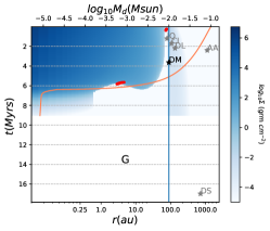
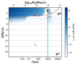
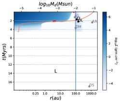
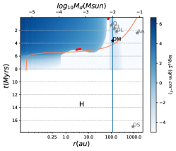
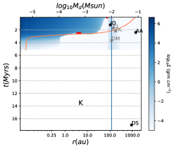
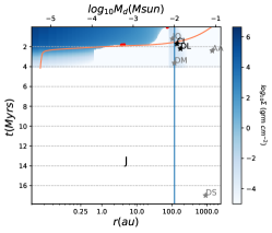
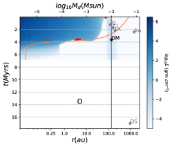
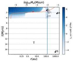
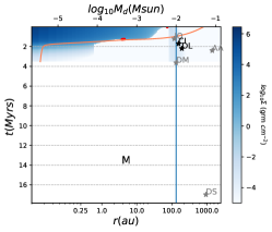
	$\xrightarrow{\makebox[170.71652pt]{$M_{*}$}}$

Figure 8: Evolution of the grid of models for a photoevaporation controlled by X-ray heating, with a wind with efficiency parameter $e_{x}=5.0$ (meaning the X-ray wind mass losses to be five times the fiducial mass rate), a viscosity value of $\alpha=10^{-4}$ and a variable flaring profile $P52$. The surface density in blue gets lighter as the disc is eroded. The red points indicate local minima in the density profiles. These are produced much earlier than when $e_{x}=1.0$, and the disc lifetimes are much shorter too.

The Figure 8 shows the results got when the previous models with viscosity $\alpha=10^{-4}$ and the flattening profile P52 (where $\upkappa=0.05$ changes to $\upkappa=0.02$) evolve subject to winds with an increased efficiency factor $e_{x}=5.0$.

The eroding of the disc is now stronger and the discs lifetimes are shorter. The most interesting fact is that the second dent and ring-like features produced in the outer part of the discs are now produced in almost all models of the grid, and much earlier than in the previous cases, at times when the disc masses $M_{d}$ are closer to the observed values. However, one must also note that the ring-like features produced when two dents or gaps exist at the same time are transient, and they may have very short lifetimes.

The disc masses can be obtained from CO measurements (Williams and Best, 2014; Miotello et al., 2016; Rosotti et al., 2017) or from the dust IR continuum flux, using an adequate dust-to-gas ratio (Lodato et al., 2017). Therefore, the observed disc masses may have systematic uncertainties because the CO ratio abundances estimation in the first case or the selection of the dust-to-gas ratio and the considered dust opacity in the second case. In any case, we take them as a reference point, and when we overlay the values corresponding to the Taurus systems, we see that they are best matched by the bottom row of the grid, which corresponds to the intermediate initial disc masses $M_{d}^{i}$.

When compared Figure 8 with the results from Figure 7, that used the fiducial efficiency $e_{x}=1.0$, one can note that with these strong winds the cavities just fully develop at the very end of the disc lifetime. We can also see that the second dent grows and develops quicker than the inner one. Finally, the third very external dent does not appear because this fast erosion.

The evolution of these models with winds of increased efficiency is quicker than the evolution of the models with less-efficient winds. This makes them to have ages more consistent with the observed disc lifetimes. We have overlaid the Taurus sample systems over our grid of models. The observed ring-like features of the real system with the smallest host stellar mass, the DM Tau system, seem to match in age with the $O,G,H$ models. Moreover, they also roughly have the adequate disc mass. However, the internal cavity observed in the real system seems to form too late in the synthetic models. Observational uncertainties in age determination, different gas-to-dust ratios and additional mechanisms are again a key issue.

The proper estimation of the age of the disc is then an important issue for proper calibration of the model. This age is an observable quantity, subject to large uncertainties, such as the selection of the star evolutionary HR track, reddening or blue excess and stellar masss. See a comparison of ages estimated by various methods in Gómez de Castro (2013) and references therein.

In which concerns the intermediate stellar masses, the IQ Tau system seems to roughly match the $T$ model when considering the production of ring-like features. Regarding the disc masses of AA Tau and DS Tau systems, they do not match with any model. However, it may happen that using a very large initial disc mass, even larger than the initial mass of model $I$, the AA Tau system may be reproduced.

Finally, regarding the largest stellar masses, the disc masses of the CI and DL Tau systems seems to be explained by the $J$ and $L$ model.

The creation of these ring-like features is interesting. Features below tens of AU around young stars that are less than $1$ Myr old would need an early formation of planets at the locations of the rings, and whether gas giant planets can form so close on such short timescale is still not clear (Helled et al., 2014), and other mechanisms as a common origin of multi-ring systems, such as snow lines, have been also under debate (Marel et al., 2018). Remarkably, our photoevaporative simulations may provide some complementary explanation to inner features below tens of AU around young stars.

$\xrightarrow{\makebox[170.71652pt]{$M_{d}$}}$
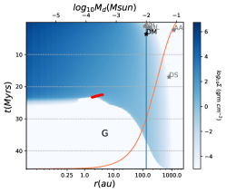
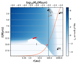
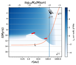
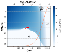
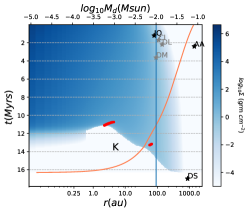
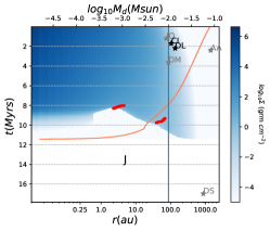
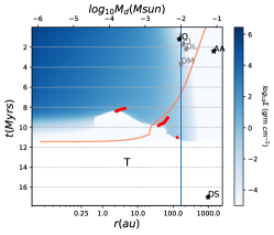
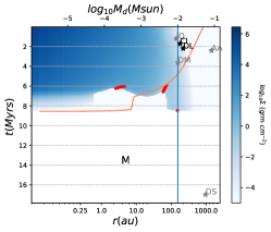
	$\xrightarrow{\makebox[170.71652pt]{$M_{*}$}}$

Figure 9: Evolution of the grid of models for a for a photoevaporation controlled by X-ray heating, with a wind with efficiency parameter $e_{x}=0.5$ (meaning the X-ray wind mass losses is half times smaller than the fiducial value), a viscosity value of $\alpha=10^{-4}$ and a variable flaring profile $P52$. The surface density in blue gets lighter as the disc is eroded. The red points indicate local minima in the density profiles. These are produced much later than when $e_{x}=1.0$, and the disc lifetimes are much longer too.

The previous results have explored very large values of the wind mass loss rates. Now, we will explore the opposite case, when the efficiency is lowered instead. The Figure 9 shows the results got when the previous models with viscosity $\alpha=10^{-4}$ and the flattening profile $P52$ evolve subject to winds with a decreased efficiency factor $e_{x}=0.5$, which corresponds to half of the fiducial mass losses.

The eroding of the disc now slows down and the discs lifetimes are much longer. This allows the formation of cavities with increased lifetimes, mainly in the smallest stellar masses. The dents and ring-like features produced in the outer part of the discs are now generated in the largest stellar mass models of the grid. These features are best seen for the lowest disc masses, where even an additional outer third dent can appear.

These features are generated when the disc masses $M_{d}$ are too low and the ages too large to match the observed values in the reference sample. However, this low efficiency $e_{x}$ value might be a way for modelling systems with very large estimated ages, like the reference system $DS$ Tau. The initial disc mass should be even larger than the initial mass of model $I$ in this case. One might also think in decreasing the flattening for making the lifetime somehow longer, slowing the erosion and creating the outer dent at proper age.

4 Photoevaporation from FUV radiation driven winds

The importance of internal FUV radiation was first analysed in Gorti and Hollenbach (2008) assuming large initial disc masses ($\approx 0.1M_{\odot}$), though external FUV heating was considered earlier in Johnstone et al. (1998) and Adams et al. (2004), producing high accretion rates. Following these models, the X-ray photons do not produce significant photoevaporation by themselves. But, because they increase the degree of ionization of the gas in the disc, there is a higher electron population which in turns reduces the positive charge of the dust grains, that helps the FUV-induced grain photoelectric heating of the gas.

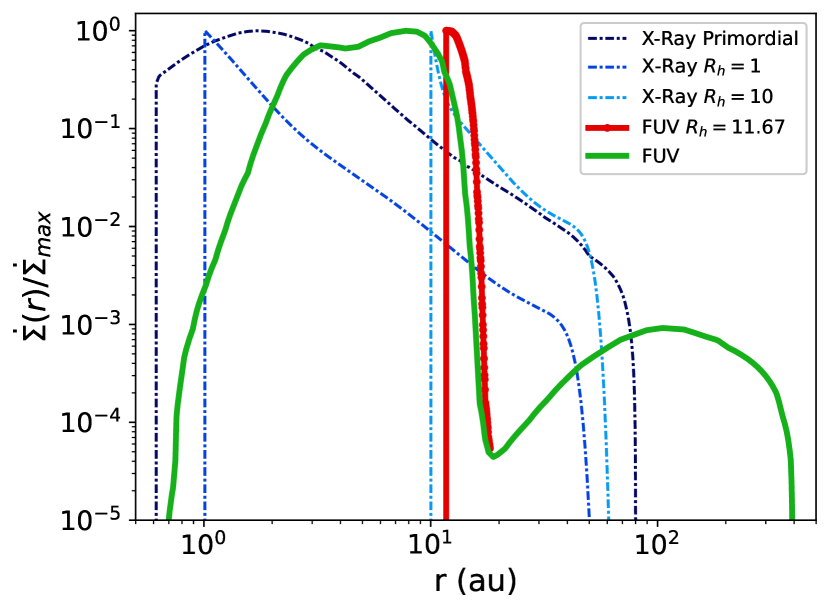
Figure 10: Normalised photoevaporative wind mass losses corresponding to the two FUV wind profiles described in Jennings et al. (2018). The FUV profile in the initial phase is a static one, meanwhile the header of the profile corresponding to the second phase is formed by a moving peak (in red) that shifts towards the position of the trough, that remains at fixed radius. At any time, the integrated mass loss is constant. The X-ray wind profiles used in Section 3 are overlaid for comparison.

We are going to consider here mass losses coming from FUV radiation to our semi-analytical $1$D model by adding the corresponding sink term to the viscous evolution in the same way we added the X-ray radiation dominated wind. We add a FUV-wind profile like the one described in Jennings et al. (2018), that is indeed developed from the models from Gorti and Hollenbach (2009).

This FUV profile, plotted in Figure 10, splits in two phases like the X-ray dominated profile seen before. There is a primordial profile, considered static, and coincident with the profile used in Gorti and Hollenbach (2009). However, the profile switches to another one when the cavity opens. Then, the inner peak initially at $7.3$au is shifted towards the trough at $18$au, keeping the profile at distances larger than $18$au unaltered. At any time, the total mass rate loss is the same that in the primordial case.

We have seen in previous section that the X-ray dominated profile mainly erodes the disc at given radii, mainly where the X-ray wind peak is located. Once this initial dent has grown so much that the floor density is reached, a gap is produced, and the inner portion of the disc is eroded until it disappears. The primordial X-ray profile peaks around $2$au, while the primordial FUV profile has a high loss between $3-10$au, peaking at around $10$au., see Figure 10. Therefore, the FUV profile may produce dents at diferent distances than the X-ray profile.

Along this work, we will keep the positions of the front and trough of the FUV profile fixed and coincident with those values from Jennings et al. (2018). Evidently, the initial position of the FUV profile might vary depending on the stellar mass and other parameters. However, in this first approach, we do not want to focus on the detailed positions of the gaps. Conversely, we aim to understand if a FUV moving front can create ring-like structures at early stages.

Hence, our key control parameter will be the FUV mass rate losses. The FUV fluxes can be generated by accretion or chromospherically, and the mass loss rate will depend on the adopted thermochemistry. As fiducial value, we have taken a mass loss rate of $3.0\cdot 10^{-8}M_{*}$ (Owen et al., 2012). However, this value may be not universal for all systems, and we will use an efficiency factor $e_{fuv}$, as we did with the X-ray dominated winds, to achieve the range of different photoevaporative mass rates discussed in Jennings et al. (2018). This $e_{fuv}$ factor will allow to reproduce the huge accretion rates close to $10^{-7}$ seen sometimes at early stages (Gorti and Hollenbach, 2009), and also the lower accretion values produced when the accretion flow may shade the disc from Lyman-$\alpha$ when it is close to the star.

$\xrightarrow{\makebox[170.71652pt]{$M_{d}$}}$
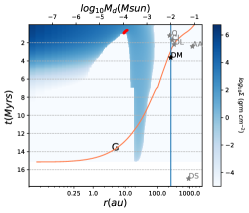
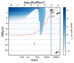
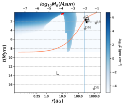
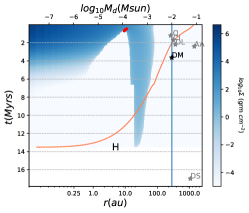
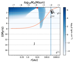
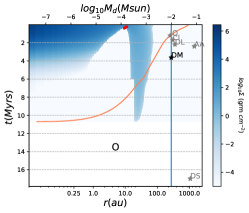
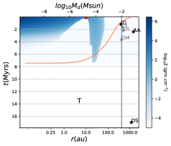
	$\xrightarrow{\makebox[170.71652pt]{$M_{*}$}}$

Figure 11: Evolution of the grid of models subject to FUV-dominated winds, with efficiency parameter $e_{fuv}=5.0$ (five times the fiducial values), a viscosity value of $\alpha=10^{-4}$ and a variable flaring profile $P52$. The surface density in blue gets lighter as the disc is eroded. The red points indicate local minima in the density profiles. The FUV wind seems to produce very good matches of the disc masses for the largest initial disc mass models. However, it creates only one inner gap that will convert into a long lasting cavity.

We first computed some simulations using this FUV-dominated wind profile using the fiducial efficiency value $e_{fuv}=1.0$. These simulations seem to create a single dent in the inner parts of the disc, around the position of the $18$au peak, which then grows and creates the inner cavity. No further dents appear, and only systems with inner cavities but no external ring-like features might be explained with these FUV-dominated models. These cavities begin to form just after a pair Myrs, but, notably, they are very long lived, lasting up to $20$Myrs in average.

Hence, the Figure 11 shows the results for simulations run with increased efficiencies $e_{fuv}=5.0$. These synthetic models open the internal cavities at earlier times. The discs lifetimes can span up to around $10$Myr for the smaller stellar masses, but makes them shorter than when $e_{fuv}=1.0$.

We have also considered lower than fiducial efficiencies, by running some simulations with $e_{fuv}=0.5$. These synthetic models reflect a much slower erosion rate, leading to really very large disc lifetimes.

5 Accretion rates

The integrated mass loss rate along all radii can be measured using the excess emission in the Balmer continuum. Even when this is a measurement that is also subject to unavoidable uncertainties, it is a fundamental parameter when studying the evolution of discs. In our models, we can compute it by integrating the surface density as follows,

$$\dot{M}=2\pi\int_{0}^{\infty}r\dot{\Sigma}(r)dr.$$ (6)

$\xrightarrow{\makebox[170.71652pt]{$M_{d}$}}$
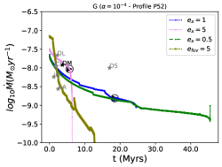
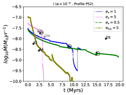
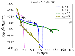
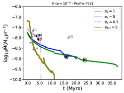
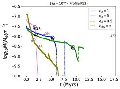
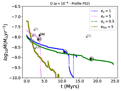
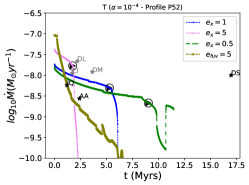
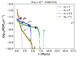
	$\xrightarrow{\makebox[170.71652pt]{$M_{*}$}}$

Figure 12: Accretion rates for X-ray winds and FUV winds, $\alpha=0.0001$ and a variable flaring profile changing from $0.05$ to $0.02$. The blue curve corresponds to the fiducial X-ray radiation dominated wind model $e_{x}=1$. The pink curve means $e_{x}=5$, and the green curve $e_{x}=0.5$. The disc subject to FUV-dominated winds, $e_{fuv}=5.0$, appears as olive curve. The black circles with a triangle within it mark when dents are present and ring-like features can be produced.

The Figure 12 shows the accretion rates in discs subject to photoevaporation from X-rays dominated or FUV-dominated winds. All curves correspond to $\alpha=10^{-4}$ and a progressive flattening $P52$. The blue curve means X-rays radiation dominated $e_{x}=1.0$, the pink curve means $e_{x}=5.0$ and the green curve means $e_{x}=0.5$. The disc subject to FUV-dominated winds, $e_{fuv}=5.0$, appears as olive curve. The black circles with a triangle within it marks when a ring-like feature is produced.

This figure shows how the initial value of the accretion rate depend on the disc mass $M_{d}$. The larger the initial disc mass, the higher the initial accretion rate. However, the later evolution of this initial value will depend on remaining control parameters.

Obviously, when comparing the evolution of discs with high and low values of the viscosity, the decay is faster and the dependency on the remaining control parameters is stronger in the case of low viscosity $\alpha$, in coincidence with the EUV-only case (Vallejo and Gómez de Castro, 2018).

If we consider the variable flaring profile $P52$, with a primordial phase starting with a higher temperature than the standard $\upkappa=0.033$, the mass rates are higher. The stronger the wind, the larger the accreted mass, with larger differences for the larger stellar masses.

In general, the mass rate decreases continuously until the first (inner) dent in the disc opens a gap. Then, the decrease in mass rate is faster meanwhile the gap widens until the inner disc is fully drained. When the inner cavity opens and the direct flux phase starts, there is in some cases an increase in the mass accretion rate. This can be explained because the photoevaporated mass rate is lower in direct flux phase than in the primordial case. Hence, the mass loss due to photoevaporation decreases, and, in turn, the accreted mass rate that remains after subtracting the wind losses is larger. However, one must also note that our models are still very simple, and further refinements when reaching the direct phase in an under flattening disc.

We have already seen in previous sections that when disc mass is very small in the direct flux phase, the front of the wind can carve an outer dent, and even an outer gap on it. These outer dents are marked by circles in Figure 12. The stronger the wind and the lower of the disc mass, the higher the likelihood of having these dents and gaps.

The models with a high viscosity $\alpha$ predict a very fast reduction in the mass rates. Conversely, the mass rates when one decreases $\alpha$ are closer to the observed values in the Taurus systems (Vallejo and Gómez de Castro, 2018). The Figure 12 shows that even taking $\alpha=10^{-4}$, the synthetic models produce mass rates slightly lower than the Taurus systems, but IQ and AA Tau.

The DM Tau seems to roughly match with several curves corresponding to different initial disc masses. The pink curve ($e_{x}=5.0$) in the $H$ model is the closest to this system. However, when we also consider when ring-like features are created, flagged by the black circle with an arrow inside, the DM Tau makes a better match in age, disc mass and accretion rate with the synthetic model with the smallest initial disc mass ($O$).

When considered FUV-dominated fluxes, the accretion rate of DM Tau is closer to the mass rate curves in $G$ model. But, when one takes into account the creation of dents, the FUV-dominated models seems to produce just the internal cavity, and no any other ring-like feature. Our models are very simple, and this may point again to further explore the parametric space.

Regarding the Taurus systems with intermediate stellar mass (panels in the central column of the figure), the IQ and AA Tau systems seem to be far away from the mass rates coming from our X-ray dominated models, and closer to those produced by FUV-dominated winds. The AA Tau system might be modelled by a synthetic system with an initial mass larger than the $I$ model. Notably, the DS Tau system seems to be far away from all plotted curves because its large age. However, we note again that we do not aim to explain all Taurus systems. Conversely, we just aim to analyse the role of the diverse model parameters in lifetimes, mass rates and ring-like features.

Notably, the FUV-dominated curve does the best match in these intermediate stellar mass systems. while predicting the proper cavity ages. However, these models, constrained by using a FUV wind with fixed peak and trough, did not predict the creation of ring-like features at any age.

Finally, in which concerns the largest stellar masses, the CI and DL Tau systems seem to match with almost any X-ray dominated model. Considering the disc mass and observed features at time, the $J$ model have a good match when considering the highest efficiency of the wind.

The curves describing the mass rate evolution also provide a view of the lifetimes of the discs. We see how these disc lifetimes depend on the stellar mass, the smaller lifetimes corresponding to the largest stellar masses. As the stellar mass increases, the accreted mass rate grows, as expected.

Notably, some of our photoevaporative models may explain objects with large inner cavities and strong accretion rates, while much simpler models fail to explain them (Ercolano et al., 2018). These transition discs with large cavities and strong accreting rates have sometimes be linked to (multiple) giant planet formation systems (Dodson and Salyk, 2011). Alternatively, following Ercolano et al. (2018), these features could result from X-ray photoevaporation in metal (C and O) depleted discs, and our models might support this photoevaporative approach.

However, we must stress again the simplicity of our models, mainly the FUV-dominated wind with fixed geometrical parameters. The best matches of the ages of our models with those from real Taurus systems are produced with very large $e_{fuv}$ values. The cavities seem to be produced in all cases, but at somehow late ages. Unfortunately, no ring-like features seems to be present in these initial analyses and further explorations of the parameter space are needed.

6 Conclusions

We have analysed the impact of a progressive flattening in protoplanetary flared discs combined with different photoevaporative winds in the creation of ring-like structures, using simple semi-analytical $1D$ $\alpha$-disc.

Previous works that used combined X-ray and FUV winds (Gorti and Hollenbach, 2009) predicted a significant population of discs with relatively massive discs and low accretion rates with large inner holes. By adding variable flaring profiles and different wind efficiencies, other combinations of accretion rates and masses are possible, as seen when we compare our results with measured parameters in real systems from Taurus.

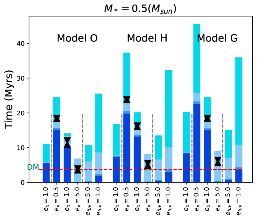
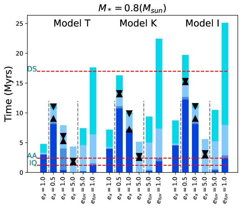
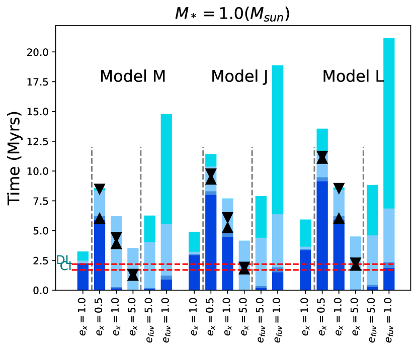
Figure 13: Summary of the evolution and lifetimes of synthetic discs. The first bar corresponds to a fiducial X-dominated wind with $\alpha=10^{-3}$, the remaining groups of bars correspond to $\alpha=10^{-4}$, the first group being an X-ray dominated wind, the second group being a FUV wind with secondary X-ray emission. The horizontal dashed lines mark the ages of the Taurus reference systems.

As summary of previous sections, the creation of ring-like structures in photoevaporative discs are facilitated in discs with low viscosity values and a flared geometry that flattens as the disc evolves. Several ring-like features can be produced with a variety of efficiencies. Up to three dents can be obtained with fiducial or weak winds, meanwhile only two dents are got with strong winds. However, the later case is the one that does not require long lifetimes until the ring-like features fully develop. Regarding the generation of long-lived cavities, these are best seen in the FUV-dominated models. However, they are also present in the X-ray dominated cases despite being very short-lived.

The Figure 13 summarises these results. Every phase appears in a different blue tone. When the inner cavity starts to develop is dark blue, when it opens is turquoise, when the direct flux starts is light blue, and the final outer disc evolution is plotted in cyan. The first bar corresponds to a fiducial X-dominated wind with $\alpha=10^{-3}$, the remaining groups of bars correspond to $\alpha=10^{-4}$, the first group being an X-ray dominated wind, the second group being a FUV wind with secondary X-ray emission. The time when the first dent appears is marked with an upper arrow. The last time when any dent (it might have or not evolved to be a gap) is present is marked with a downward arrow.

The Figure 13 also provides the different disc lifetimes of the grid models. When the wind efficiencies increase, the lifetimes are shortened. In this figure one can also observe than these lifetimes decrease with the host star mass, and when we fix this parameter, lifetimes grow with initial disc mass, as expected.

The age when the gas is depleted constrains the potential ending of the formation of gas giants planets, and migration processes that involve exchanges of angular momentum could also stop at these early ages (Alexander and Armitage, 2009). We have seen that one can achieve very short disc lifetimes when using winds with high efficiency factors.

A FUV-dominated photoevaporative wind seems to reproduce well the accretion rates found in the intermediate stellar mass cases of our limited sample, but fails in reproducing the ring-like features at inner and outer distances observed in real systems, and only produce cavities of slow evolution. Conversely, with X-ray dominated winds, one gets gaps in the range of tens of astronomical units in discs as young as $1$ Myr old.

Therefore, a progressive flattening of the disc seems to support the production of ring-like features at the observed ages. These features can be produced in our synthetic models when two dents or gaps exist at the same time. Hence, our ring-like features are transient features, typically lasting less than $1$Myr. Notably, a third dent can appear, more likely in the higher stellar masses and higher disc masses models. However, it does not coincide in time with the previously generated dents.

All these features are transient, and they are roughly coincident with some of the annular features seen in a few of the Taurus disc of our sample (see Table 1) when using somehow too strong efficiencies.

The major part of these ring-like features are only created before the internal cavity is fully developed. The timescales for the creation of internal cavities do not match well and further explorations of the involved parameters are still needed. One improvement should be to modify some of the geometrical baseline parameters of our wind profiles, such as the peak and trough of the FUV profile at fixed positions used in this work. Another important enhancement should be to further refine the flattening process.

Moreover, some additional mechanism may be needed for carving faster the dents and create real gaps. For instance, our dents may convert onto dust traps, accelerating the process of gaps creation in a similar fashion that the gaps creation mechanisms is attributed to planets. Despite of that, our simple photoevaporative dents still may produce valid predictions, considering that the dents may trigger this mechanism and lead to the observed structures.

We note that we have just considered the evolution of the gas, and its evolution can be somehow different than the evolution of the dust, even when the initial dents created by photoevaporative processes may indicate dents into the dust. One also may take into account observational uncertainties. The gas, mainly $H_{2}$ ($90$%) and He ($10$%), is difficult to observe, and typically one uses CO ( $0.01$%) as a proxy (Miotello et al., 2016; Molyarova et al., 2017). But CO can have a complex distribution due to the disk structure hence making the interpretation of the results very difficult, leading to the analysis of other tracers that are even more scarce (Williams and Best, 2014).

Many other observations are based on dust continuum, where discs present rings and gaps, in addition to the internal cavity. The gas surface density is assumed to follow the dust density evolution, driven by a given dust-to-gas ratio (Birnstiel et al., 2010). Certainly, this may not be true, and the dust-to-gas mass ratio be a free parameter. Anyhow, if gas might be much abundant than dust, one may find that meanwhile gas erosion keeps as a small dent, dust may have already formed a gap. If this ratio changes with time or is not constant along the disc (see, for instance Birnstiel et al. (2010)), it might be higher in the outer parts of the disc than in the inner side, making the outer features in the dust to appear before than in the gas.

We have seen that the disc mass evolution curves, the accretion rates curves and the mass density features predicted by our models can sometimes resemble those found in the reference Taurus systems. This supports the usefulness of using $1D$ models because their simplicity in interpreting their results. These results can be summarised in Figure 14. Here, we can see a schematised view of the position of the ring-like features, inner cavities and gaps, of different widths produced by the grid models. Some of the model-generated features resemble those observed in the Taurus reference sample (denoted by red dashed lines) at proper ages.

The best matches are got with IQ Tau, CI Tau and DL Tau. Their ages, disc masses and accretion rates can be reproduced, while one can see structures resembling to those seen in some of those real systems. However, very high mass losses are needed, and some additional gaps should be carved for having a better match.

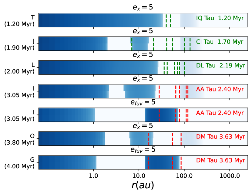
Figure 14: A schematised view of the position of the ring-like features, inner cavities and gaps, of different widths produced by the grid models. The first three models produce features resembling those observed in the Taurus reference sample at the proper age, with a disc mass and accretion rate similar to the observed values. These Taurus features appear as dashed lines, red color indicating the internal cavity is present. The last three models produce a gap at proper ages, but the cavities are fully developed much later than when observed in real systems. Note that the colorscale denotes the model surface density.

Obviously, there are limitations in such simplifications. Our simple models do not reproduce other reference real systems. The synthetic models closer to DM Tau and AA Tau are still eroding the internal cavity, while the real DM Tau and AA Tau have already developed this cavity. By other hand, DS Tau seems to remain out of any of our model predictions, even when DS Tau may be matched with a model with initial mass larger than $I$ model, may be using a very inefficient X-ray dominated wind.

Observations of inner ring-like structures very close to the host star are not straightforward and remain somehow elusive below the astronomical unit. Our baseline models focused on low viscosity values in order to better match with measured disc ages. However, the disc composition is not the only source for shortening discs lifetimes. We have seen the important role played by the flattening of the disc profile. Therefore, a quite interesting research topic that can extend the results presented here is to modify further the geometrical baseline parameters of the flaring profiles and the flattening process, especially in the case of FUV-dominated winds. These enhancements may change the location and time where cavities, dents and gaps are created.

Data availability

The data underlying this article will be shared on reasonable request to the corresponding author.

References

- Adams et al. (2004) Adams, F.C., Hollenbach, D., Laughlin, G., Gorti, U., 2004, ApJ, 611, 360.
- Adams et al. (2012) Adams, F.C., Fatuzzo, M., Holden, N., 2012, PASP, 124, 913.
- Alexander et al. (2006) Alexander, D., Clarke, C.J. and Pringle, J.E., 2006, MNRAS, 369, 229.
- Alexander (2007) Alexander, D., 2007, MNRAS, 375, 500.
- Alexander and Armitage (2009) Alexander, D., Armitage, P.J., 2009, ApJ, 704, 989.
- Anderson et al. (2013) Anderson, K.R., Adams, F.C., and Calvet, N., 2013, ApJ, 774, 49.
- Andrews et al. (2009) Andrews, S.M., Wilner, D.J., Hughes, A.M., Qi, C., Dullemond, C.P., 2009, ApJ, 700, 1592.
- Andrews et al. (2011) Andrews, S.M., Rosenfeld, K.A., Wilner, D.J., Bremer, M., 2011, ApJ, 742, 5A.
- Andrews et al. (2018) Andrews, S.M. et al., 2018, ApJ, 869L, 41A.
- Andrews (2020) Andrews, S.M., 2020, Annual Review of Astronomy and Astrophysics, 58, 483.
- Armitage and Hansen (1999) Armitage P. J., Hansen B. M. S., 1999, Nature, 402, 633.
- Armitage (2015) Armitage, P.J., 2015, arXiv:1509.06382.
- Balbus and Hawley (1991) Balbus, S.A, Hawley, J.F., 1991, ApJ, 376, 214.
- Bai (2016) Bai, X., 2016, ApJ, 821, 80.
- Barge et al. (2017) Barge, P., Ricci, L., Carilli, C.L., Previn-Ratnasingam, R., 2017, A&A, 605A, 122B.
- Bertout et al. (2007) Bertout, C., Siess, L., & Cabrit, S. A&A, 473, L21
- Birnstiel et al. (2010) Birnstiel, T., Dullemond, C.P. and Brauer, F., 2010, A&A 513, A79.
- Boley (2017) Boley, A.C., 2017, ApJ, 850, 103B.
- Chiang and Goldreich (1997) Chiang, E., Goldreich, P, 1997, ApJ, 490, 368.
- Chiang et al. (2001) Chiang, E.I., Joung, M.K., Creech-Eakman, M.J., Qi, C., Kessler, J.E., Blake, G.A., van Dishoeck, E.F., 2001, ApJ, 547, 1077.
- Clarke et al. (2001) Clarke, C.J., Gendrin, A. and Sotomayor, M., 2001, MNRAS, 328, 485.
- Concha-Ramirez et al. (2019) Concha-Ramirez, F., Wilhelm, M.J.C., Portegies, S., Haworth, T.J. , 2019, MNRAS, 490, 5678C.
- DAlessio et al. (1999) D’Alessio P., Calvet N., Hartmann L., Lizano S., Cantó J., 1999, ApJ,527,93.
- Dullemond and Dominik (2004) Dullemond, C.P., Dominik, C., 2004, A&A, 421,1075.
- Dullemond and Dominik (2005) Dullemond, C.P., Dominik C., 2005, A&A, 434, 971.
- Dodson and Salyk (2011) Dodson-Robinson, S.E., Salyk, C., 2011, ApJ, 738, 131D.
- Dong et al. (2015) Dong, R., Zhu, Z., Rafikov, R.R., Stone, J.M., 2015, ApJ, 809, 5D.
- Doucet et al. (2007) Doucet, C., Habart, E., Pantin, E., et al., 2007, A & A, 470, 625.
- Ercolano and Rosotti (2015) Ercolano B., Rosotti, G., 2015, MNRAS, 450, 3008.
- Ercolano et al. (2017) Ercolano, B., Jennings, J., Rosotti, G., Birnstiel, T., 2017, MNRAS, 472, 411.
- Ercolano et al. (2018) Ercolano, B., Weber, M.L., Owen, J.E., 2018, MNRAS, 473L, 64E.
- Espaillat (2014) Espaillat, C., Muzerolle, J., Najita, J., Andrews, S., Zhu, Z., Calvet, N., Kraus, S., Hashimoto, J., Kraus, A., DAlessio, P., 2014, An Observational Perspective of Transitional Disks, Protostars and Planets VI, Beuther H., Klessen, R.S., Dullemond C.P. and Henning T. (eds.), University of Arizona Press, Tucson, 914 pp., p.497-520.
- Francis and van der Marel (2020) Francis, L., van der Marel, N., 2020, ApJ, 892, 111F.
- Gómez de Castro and Marcos-Arenal (2012) Gómez de Castro, A.I., Marcos-Arenal, P., 2012, ApJ, 749, 190G.
- Gómez de Castro (2013) Gómez de Castro, A.I., 2013, Planets, Stars and Stellar Systems Vol. 4, by Oswalt, T.D., Barstow, M.A., Springer Science+Business Media Dordrecht, 2013, p. 279.
- Gonzalez et al. (2017) Gonzalez, J.F., Laibe, G., Maddison, S.T., 2017, MNRAS, 467, 1984G.
- Gorti and Hollenbach (2008) Gorti, U., Hollenbach, D., 2008, ApJ, 683, 287G.
- Gorti and Hollenbach (2009) Gorti, U., Hollenbach, D., 2009, ApJ, 690, 1539.
- Grassi et al. (2020) Grassi, T., Ercolano, B., Szücs, L., Jennings, J., Picogna, G., 2020, MNRAS, 494, 4471G.
- Güdel et al. (2007) Güdel M., Güdel, M., Briggs, K.R., Arzner, K., Audard, M., Bouvier, J., Feigelson, E.D., Franciosini, E., Glauser, A., Grosso, N., Micela, G., Monin, J.L., Montmerle, T., Padgett, D.L., Palla, F., Pillitteri, I., Rebull, L., Scelsi, L., Silva, B., Skinner, S.L., Stelzer, B., Telleschi, A. , 2007, A & A, 468, 353.
- Hartmann et al. (1998) Hartmann L., Calvet, N., Gullbring, E., and D’Alessio, P., 1998, ApJ, 495, 385.
- Hartmann (2000) Hartmann L., 2000, ESASP, 445, 107H.
- Hartmann and Bae (2018) Hartmann L., Bae, J., 2018, MNRAS, 474, 88.
- Hawley and Balbus (1995) Hawley, J.F., Balbus, S.A., 1995, PASA, 12, 159H.
- Helled et al. (2014) Helled, R., Bodenheimer, P., Podolak, M., et al., 2014, Protostars and Planets VI, 64
- Heinemann and Papaloizou (2009) Heinemann, T., Papaloizou, J.C.B. , 2009, MNRAS, 397, 64.
- Hollenbach (1994) Hollenbach, D., Johnstone, D., Lizano, S. and Shu, F., 1994, ApJ, 428, 654.
- Huang et al. (2018) Huang, J., Andrews, S.M., Perez, L.M., Zhu, Z., Dullemond, C.P., et al, 2018, ApJ, 869, 43H.
- Johnstone et al. (1998) Johnstone, D., Hollenbach, D., Bally, J., 1998, ApJ, 499, 758J.
- Kimura et al. (2016) Kimura, S.S., Kunitomo, N., Takahashi, S.Z., 2016, MNRAS, 461, 2257.
- Jennings et al. (2018) Jennings, J., Ercolano, B., and Rosotti, G.P., 2018, MNRAS, 477, 131.
- Jones et al. (2012) Jones, M.G., Pringle, J.E., Alexander, R.D., 2012, MNRAS, 419, 925.
- Kratter and Lodato (2016) Kratter, K., Lodato, G., 2016, ARA&A, 54, 271..
- Lodato et al. (2017) Lodato, G., Scardoni, Ch.E., Manara, C.F., Testi, L., 2017, MNRAS, 472, 4700.
- Lodato et al. (2019) Lodato, G., Dipierro, G., Ragusa, E., et al, 2019, MNRAS, 486, 453L .
- Long et al. (2018) Long F., Pinilla P., Herczeg, G.J., Harsono, D., et al, 2018, ApJ, 869, 17.
- Long et al. (2020) Long F., Pinilla P., Herczeg, G.J., Andrews, S.M., et al, 2020, ApJ, 898, 36L.
- Luhman (2018) Luhman, K. L. AJ, 156, 271
- Lynden-Bell and Pringle (1974) Lynden-Bell, D, Pringle, J.E., 1974, MNRAS, 168, 603.
- Marel et al. (2018) van der Marel, N. , Dong, R. , di Francesco, J. , Williams, J.P., Tobin, J., 2019, ApJ, 872, 112V.
- Martin et al. (2019) Martin R.G., Nixon, C.J., Pringle, J.E., Livio M., 2019, NewA, 70, 7M.
- Maaskant et al. (2013) Maaskant, K.M., Honda, M., Waters, L.B.F.M., et al, 2013, A & A, 555A, 64M.
- Miotello et al. (2016) Miotello, A., van Dishoeck, E.F., Kama, M., Bruderer, S., 2016, A & A, 594A, 85M.
- Molyarova et al. (2017) Molyarova, T., Akimkin, V., Semenov, D., Henning, T., Vasyunin, A. and Wiebe, D., 2017, ApJ, 849, 2.
- Nakatani et al. (2018) Nakatani, R., Hosokawa, T., Yoshida, N., Nomura, H., Kuiper, R., 2018, ApJ, 865, 75N.
- Okuzumi et al. (2016) Okuzumi, S., Momose, M., Sirono, S., Kobayashi, H. Tanaka, H., 2016, ApJ, 821, 82O .
- Owen et al. (2012) Owen, J.E., Clarke, C.J. and Ercolano, B., 2012, MNRAS, 422, 1880.
- Papaloizou (2005) Papaloizou, J. C. B., 2005, CeMDA, 91, 33P.
- Picogna et al. (2019) Picogna, G., Ercolano, B., Owen, J.E., Weber, M.L., 2019, A&A, 617, A117.
- Pudritz et al. (1991) Pudritz, R., Pelletier, G, Gómez de Castro A.I., 1991, The Physics of Star Formation and Early Stellar Evolution, NATO Advanced Study Institute (ASI) Series C, Vol. 342, held in Agia Pelagia, Crete, Greece, May 27th - June 8th, Dordrecht: Kluwer, 1991, edited by Charles J. Lada and Nikolaos D. Kylafis., p.539.
- Riols and Lesur (2018) Riols, A., Lesur, G., 2018, A&A, 617, A117.
- Rometsch et al. (2020) Rometsch, T., Rodenkirch, P.J., Kley, W., Dullemond, C.P., 2020, A&A, 643, A87.
- Rosotti et al. (2013) Rosotti, G., Ercolano, B, Owen, J. Armitage, P., 2013, MNRAS, 430, 1392.
- Rosotti et al. (2017) Rosotti, G.P., Clarke, C.J., Manara, C.F., Facchini, S., 2017, astro-ph.SR 8 Mar 2017.
- Ruge et al. (2016) Ruge, J. P., Flock, M., Wolf, S., Dzyurkevich, N., Fromang, S., Henning, Th., Klahr, H., Meheut, H., 2016, A&A, 590A, 17R.
- Shakura and Sundayev (1973) Shakura, N.I., Sundayev, R.A., 1973, A&A, 24, 337.
- Shakura and Sundayev (1976) Shakura, N.I., Sundayev, R.A., 1976, MNRAS, 175, 613.
- Simon et al. (2017) Simon, M., Guilloteau, S., Di Folco, E., et al, 2017, ApJ, 844, 158S.
- Suriano et al. (2018) Suriano, S., Li, Z., Krasnopolsky, R., Shang, H., 2018, MNRAS, 477, 1239S.
- Takahashi and Inutsuka (2016) Takahashi, S.Z., Inutsuka, S., 2016, AJ, 152, 184.
- Tazzari et al. (2017) Tazzari M., Testi, L., Natta, A., Ansdell, M., et al., 2017, A&A, 606,A88,
- Telleschi (2007) Telleschi, et al, 2007, A&A, 468, 425.
- Ustamujic et al. (2016) Ustamujic, S., Orlando, S., Bonito, R., Miceli, M., Gómez de Castro, A. I., López-Santiago, J., 2016, A&A, 596, 99.
- Vallejo and Gómez de Castro (2018) Vallejo, J.C., Gómez de Castro, A.I., 2018, APSS, 363, 246.
- Wang and Goodman (2017) Wang, L. and Goodman, J., 2017, ApJ, 847, 11W.
- Williams and Cieza (2011) Williams, J.P., Cieza, L.A., 2011, Annual Review of AA,49,67.
- Winter et al. (2018) Winter, A.J., Clarke, C.J., Rosotti, G., Ih, J., Facchini, S., Haworth, T. J., 2018, MNRAS, 478, 2700W.
- Williams and Best (2014) Williams, J.P. and Best, W.M.J., 2014, ApJ, 788, 59.
- Wolfer et al. (2019) Wolfer, L., Picogna, G., Ercolano, B., van Dishoeck, E.F., 2019, MNRAS, 490, 5596W.
- Zhang and Jin (2015) Zhang, Y., Jin, L., 2015, ApJ, 802, 58Z.