Nonlinearity-induced transition
in nonlinear Su-Schrieffer-Heeger model and nonlinear higher-order topological system

Abstract

We study the topological physics in nonlinear Schrödinger systems on lattices. We employ the quench dynamics to explore the phase diagram, where a pulse is given to a lattice point and we analyze its time evolution. There are two system parameters $\lambda$ and $\xi$, where $\lambda$ controls the hoppings between the neighboring links and $\xi$ controls the nonlinearity. The dynamics crucially depends on these system parameters. Based on analytical and numerical studies, we derive the phase diagram of the nonlinear Su-Schrieffer-Heeger (SSH) model in the ($\lambda,\xi$) plane. It consists of four phases. The topological and trivial phases emerge when the nonlinearity $\xi$ is small. The nonlinearity-induced localization phase emerges when $\xi$ is large. We also find a dimer phase as a result of a cooperation between the hopping and nonlinear terms. A similar analysis is made of the nonlinear second-order topological system on the breathing Kagome lattice, where a trimer phase appears instead of the dimer phase.

I Introduction

Topological phases have attracted much attention in the context of solid state materialsHasan ; Qi with the emergence of topological edge states. They are generalized to higher-order topological phasesFan ; Science ; APS ; Peng ; Lang ; Song ; Bena ; Schin ; FuRot ; EzawaKagome ; Khalaf , where topological corner states and topological hinge states emerge. Recently, they are also found in various linear systems such as photonicKhaniPhoto ; Hafe2 ; Hafezi ; WuHu ; TopoPhoto ; Ozawa16 ; Ley ; KhaniSh ; Zhou ; Jean ; Ota18 ; Ozawa ; Ota19 ; OzawaR ; Hassan ; Ota ; Li ; Yoshimi ; Kim ; Iwamoto21 , acousticProdan ; TopoAco ; Berto ; Xiao ; He ; Abba ; Xue ; Ni ; Wei ; Xue2 , mechanicalLubensky ; Chen ; Nash ; Paul ; Sus ; Sss ; Huber ; Mee ; Kariyado ; Hannay ; Po ; Rock ; Takahashi ; Mat ; Taka ; Ghatak ; Wakao and electric circuitTECNature ; ComPhys ; Hel ; Lu ; YLi ; EzawaTEC ; Research ; Zhao ; EzawaLCR ; EzawaSkin ; Garcia ; Hofmann ; EzawaMajo ; Tjunc ; Lee ; Kot systems. Now, nonlinear topological photonics is an emerging fieldLey ; Zhou ; Smi ; Kruk ; MacZ , where nonlinearity is naturally introduced by the Kerr effect. Nonlinear higher-order topological phases have been experimentally studied in photonicsZange ; Kirch . Topological edge states and topological corner states have been observed in nonlinear systems just as in linear systems.

It is a hard task to construct a general theory of the topological physics in nonlinear systems because there are many ways to introduce nonlinearity. It would be necessary to make individual studies of typical nonlinear models to achieve at a systematic understanding. We studied the dimerized Toda-lattice modelTopoToda and a nonlinear mechanical systemMechaRot in previous works. These models contain the Su-Schrieffer-Heeger (SSH) model as an essential term. Indeed, these models are reduced to the dynamical SSH model provided the nonlinear term is ignored, where the topological number is well defined and the zero-mode edge state emerges in the topological phase. Then, we carried out numerical analysis to show the topological physics is valid even in the presence of the nonlinear term. These models have only two phases, the topological phase and the trivial phase in the phase diagram in the ($\lambda,\xi$) plane, with $\lambda$ the dimerization parameter and $\xi$ the nonlinearity parameter.

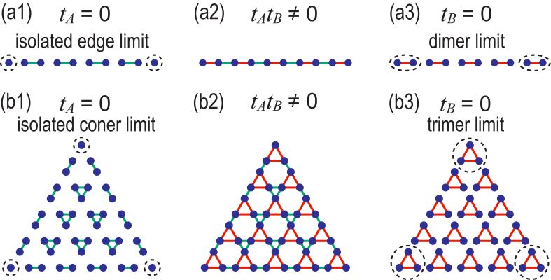
Figure 1: Illustration of (a) a dimerized lattice and (b) a breathing Kagome lattice with (a) $t_{A}=0$, (b) $t_{A}t_{B}\neq 0$ and (c) $t_{B}=0$. A line (triangle) contains many small segments (triangles). At the edges (corners) of the chain (triangle), there are two (three) isolated atoms for $t_{A}=0$, while there are dimer (trimer) states for $t_{B}=0$. They are marked by dotted circles. The size of the line (triangle) is $L=5$.

In this paper, we study the quench dynamics governed by a nonlinear Schrödinger equation consisting of the hopping term with the hopping matrix $M_{nm}$ and the nonlinear term proportional to the nonlinearity parameter $\xi$. In the quench dynamics, we give a pulse to a lattice point and explore its time evolution. The dynamics is sensitive to the presence of the topological edge and corner states. We perform a numerical analysis in a wide region of parameters and construct phase diagrams in the ($\lambda,\xi$) plane. We are interested in the systems which describe nontrivial topological dynamics in the linear limit ($\xi=0$). As explicit examples, we take $M_{nm}$ on the SSH lattice and on the breathing Kagome lattice. We confirm analytically the validity of the topological dynamics in the weak nonlinearity regime ($\xi\ll 1$) based on the first-order perturbation theory in $\xi$. We show that the topological phase boundary between the topological and trivial phases is well defined and not modified in this weak nonlinearity regime. In the strong nonlinearity regime ($\xi\gg 1$) where the nonlinear term is dominant, we obtain analytically the nonlinearity-induced localization phase, where the state is localized due to the nonlinear term. It is unrelated to the topological physics because the term $M_{nm}$ is irrelevant in this regime. The transition from the weak to the strong nonlinearity regime is a transition from extended states to localized states. We have also found a new phase formed by a cooperative effect of these two terms, which is the oscillation-mode phase in the vicinity of the dimerized nonlinear SSH model and the trimerized breathing Kagome model illustrated in Fig.1(a3) and (b3), respectively.

This paper is composed as follows. In Section II, we review the nonlinear Schrödinger equation. We discuss it analytically in the linear limit ($\xi=0$), in the weak nonlinearity regime ($\xi\ll 1$) and in the strong nonlinearity regime ($\xi\gg 1$). We find that the topological phase transition point does not change in the weak nonlinear regime. On the other hand, the system turns into the nonlinearity-induced localization phase in the strong nonlinearity regime. In Section III, we explicitly study the nonlinear SSH model, where the phase diagram is determined by a numerical analysis. It consists of the topological phase, the trivial phase, the nonlinearity-induced localization phase and the dimer phase. We discuss the origin of the dimer phase as an operative effect of the hopping term and the nonlinear term. In Section IV we explicitly study the nonlinear second-order topological phase on the breathing Kagome lattice, where the phase diagram is constructed by a numerical analysis. The analysis and the results are quite similar to those in the nonlinear SSH model except for the trimer phase replacing the dimer phase.

II Nonlinear Schrödinger equation

A typical nonlinear equation is the nonlinear Schrödinger equation,

$$i\frac{\partial\psi}{\partial t}+\varepsilon\frac{\partial^{2}\psi}{\partial x^{2}}+\xi\left|\psi\right|^{2}\psi=0,$$ (1)

where the third term is a nonlinear term. It is introduced by the Kerr effect in the case of photonic systemsSzameit ; Chris . The nonlinearity is controlled by the parameter $\xi$, where large $\xi$ indicates strong nonlinearity. There is a lattice version of the above equation,

$$i\frac{d\psi_{n}}{dt}+\varepsilon\left(\psi_{n+1}-2\psi_{n}+\psi_{n-1}\right)+\xi\left|\psi_{n}\right|^{2}\psi_{n}=0,$$ (2)

which is called the discrete nonlinear Schrödinger equationCai ; Kev . There are two conserved quantities. One is the HamiltonianEil ; Szameit ; Korab ,

$$H=\sum_{n=1}^{N}\left(\varepsilon\left|\psi_{n+1}-\psi_{n}\right|^{2}-\frac{\xi}{2}\left|\psi_{n}\right|^{4}\right).$$ (3)

and the other is the excitation number,

$$N_{\text{exc}}=\sum_{n=1}^{N}\left|\psi_{n}\right|^{2}.$$ (4)

The discrete nonlinear Schrödinger equation (2) is defined on the one-dimensional lattice. It is generalized to a nonlinear equation on an arbitrary latticeEil ; Szameit ; Chris ,

$$i\frac{d\psi_{n}}{dt}+\sum_{m=1}^{N}M_{nm}\psi_{m}+\xi\left|\psi_{n}\right|^{2}\psi_{n}=0,$$ (5)

where $M_{nm}$ represents a hopping matrix, and $N$ is the number of the lattice sites. We investigate such a system that contains the topological and trivial phases provided the nonlinear term is ignored. We study analytically and numerically the phase diagram of the model (5). The main issue is how the topological phase defined in the linear model ($\xi=0$) is robust against the introduction of the nonlinear term.

There are two conserved quantitiesKorab . One is the Hamiltonian

$$H=\sum_{n=1}^{N}\left(-M_{nm}\psi_{n}^{\ast}\psi_{m}-\frac{\xi}{2}\left|\psi_{n}\right|^{4}\right),$$ (6)

and the other is the excitation number (4).

We analyze the quench dynamics by imposing an initial condition

$$\psi_{n}\left(t\right)=\delta_{n,m}\qquad\text{at}\qquad t=0.$$ (7)

Namely, giving an delta-function type input at the site $m$ initially, we study its time evolution. Because of the conservation rule (4), the condition

$$\sum_{n=1}^{N}\left|\psi_{n}\right|^{2}=1$$ (8)

is imposed throughout the time evolution.

A comment is in order. It is possible to eliminate the nonlinearity parameter $\xi$ entirely from Eq.(5). By setting $\psi_{j}=\psi_{j}^{\prime}/\sqrt{\xi}$, we may rewrite (5) as

$$i\frac{d\psi_{n}^{\prime}}{dt}+\sum_{m}M_{nm}\psi_{m}^{\prime}+\left|\psi_{n}^{\prime}\right|^{2}\psi_{n}^{\prime}=0.$$ (9)

The initial condition (7) is replaced by

$$\psi_{n}^{\prime}\left(t=0\right)=\sqrt{\xi}\delta_{n,m}.$$ (10)

Namely, the quench dynamics subject to Eq.(5) is reproduced by the nonlinear equation (9) with the modified initial condition (10). Consequently, it is possible to use a single sample to investigate the quench dynamics at various nonlinearity $\xi$ only by changing the initial condition as in (10). Nevertheless, we use the form of Eq.(5) throughout the paper to make the nonlinear effect manifest.

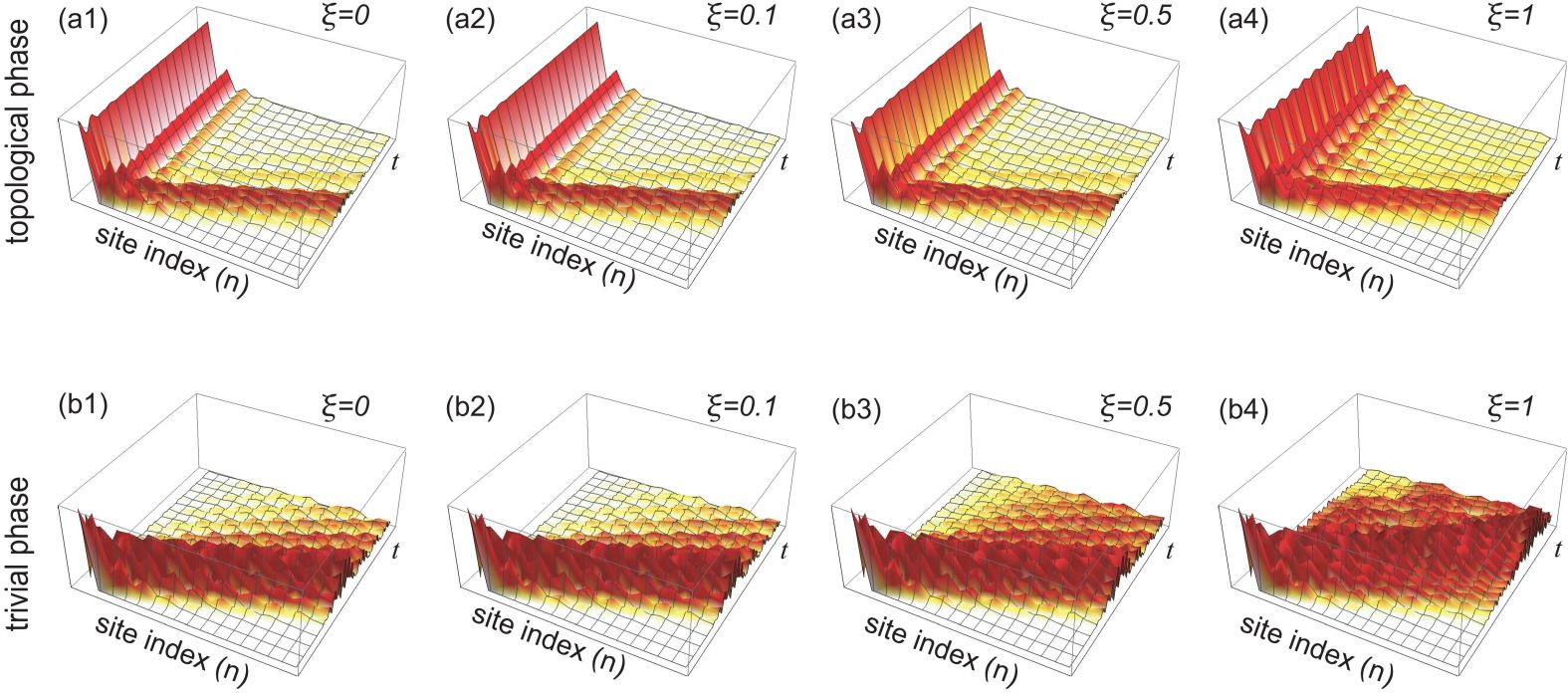
Figure 2: Bird’s eye’s view of time evolution of the amplitude $|\psi_{n}|$ in the nonlinear SSH model. The horizontal axes are the site index $n$ and the time $t$ ranging $0\leq t\leq 30$. (a1)$\sim$(a4) Topological phase ($\lambda=-0.5$). (b1)$\sim$(b4) Trivial phase ($\lambda=0.5$). We have set $\xi=0$ for (a1) and (b1), $\xi=0.1$ for (a2) and (b2), $\xi=0.5$ for (a3) and (b3), and $\xi=1$ for (a4) and (b4).

II.1 Linearized model

We first study the linear limit by setting $\xi=0$,

$$i\frac{d\psi_{n}}{dt}+\sum_{m}M_{nm}\psi_{m}=0.$$ (11)

We diagonalize $M_{nm}$ as

$$M\bar{\psi}_{p}=E_{p}\bar{\psi}_{p},$$ (12)

where $p$ labels the eigen index, $1\leq p\leq N$. Then, we obtain decoupled equations

$$i\frac{d\bar{\psi}_{p}}{dt}+E_{p}\bar{\psi}_{p}=0,$$ (13)

whose solutions are given by

$$\bar{\psi}_{p}\left(t\right)=\exp\left[-itE_{p}\right]\bar{\psi}_{p}\left(0\right).$$ (14)

The initial state is expanded as

$$\psi_{n}\left(0\right)=\delta_{n,m}=\sum_{p}c_{p}\bar{\psi}_{p}\left(0\right).$$ (15)

Because Eq.(11) is a linear model, the topological numbers defined with respect to $M_{nm}$ determines the topological phases of the system.

There are localized states in a topological phase known as zero-mode edge states in the one-dimensional topological phase and zero-mode corner states in the two-dimensional second-order topological phase. We impose the initial condition (7) with $m=1$, or

$$\psi_{n}\left(0\right)=\delta_{n,1},$$ (16)

where the site $n=1$ denotes the left edge of a chain or the top corner of a triangle. The zero-mode edge (corner) state is given in terms of an eigenstate of $M_{nm}$, which we assume to be $\bar{\psi}_{1}$ with $E_{1}=0$ in (12). With the use of the expansion (15), the zero-mode edge (corner) state $\bar{\psi}_{1}$ is well approximated by $\psi_{1}$ at $t=0$, or

$$\psi_{1}\left(0\right)\simeq c_{1}\bar{\psi}_{1}\left(0\right).$$ (17)

Since the zero-mode edge (corner) state has the zero energy, there is no dynamics,

$$\psi_{1}\left(t\right)=c_{1}\bar{\psi}_{1}\left(0\right).$$ (18)

As a result, there remains a finite component $c_{1}$ at the edge (corner) site even after time evolution.

On the other hand, there is no zero-mode localized state at the edge (corner) in the trivial phase, and the state $\psi_{n}\left(t\right)$ rapidly penetrates into the bulk. Consequently, it is possible to differentiate the topological and trivial phases numerically by checking whether there remains a finite component or not under the initial condition (16).

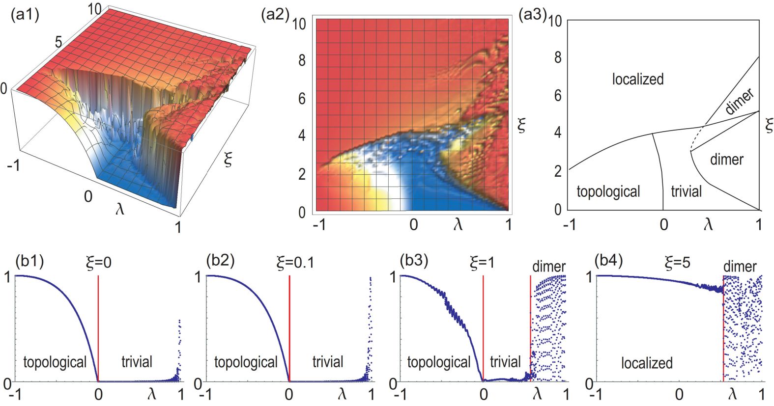
Figure 3: (a1)$\sim$(a3) Phase diagram of the nonlinear SSH model. (a1) Bird’s eye’s view, (a2) top view and (a3) schematic illustration of the phase diagram. (b1)$\sim$(b4) Amplitude $|\psi_{1}|$ as a function of $\lambda$ for various $\xi$. (b1) $\xi=0$, (b2) $\xi=0.1$, (b3) $\xi=1$, and (b4) $\xi=5$.

II.2 Weak nonlinear regime

We study the weak nonlinear regime of Eq.(5), which is the regime where the first-order perturbation in $\xi$ is valid. We may insert the linear solution (14) to the nonlinear term proportional to $\xi$ in Eq.(5), i.e.,

$$\xi\left|\psi_{n}(t)\right|^{2}\psi_{n}(t)=\xi\left|\psi_{n}\left(0\right)\right|^{2}\psi_{n}(t)+O(\xi^{2}),$$ (19)

and obtain

$$i\frac{d\psi_{n}}{dt}+\sum_{m}\overline{M}_{nm}\psi_{m}=0,$$ (20)

where

$$\overline{M}_{nm}\equiv M_{nm}+\delta_{nm}\xi\left|\psi_{n}\left(0\right)\right|^{2}.$$ (21)

The second term $\delta_{nm}\xi\left|\psi_{n}\left(0\right)\right|^{2}$ may be regarded as an on-site random potential in the linearized model. Then, the topological phase is robust against the on-site potential as far as the bulk gap does not close or equivalently $\xi\left|\psi_{n}\left(0\right)\right|^{2}$ is smaller than the gap of $M_{nm}$. Consequently, in the weak nonlinearity regime, the topological number is well defined, and the topological phase boundary is unchanged as $\xi$ increases. See explicit examples in Sec.III and Sec.IV, where the topological phase diagrams are numerically constructed.

II.3 Strong nonlinear regime

We next study the strong nonlinear regime ($\xi\gg 1$), which is the regime where the hopping term is negligible with respect to the nonlinear term. We may approximate Eq.(5) as

$$i\frac{d\psi_{n}}{dt}=-\xi\left|\psi_{n}\right|^{2}\psi_{n},$$ (22)

where all equations are separated. We set

$$\psi_{n}\left(t\right)=r_{n}e^{i\theta_{n}\left(t\right)},$$ (23)

and make an ansatz that $r_{n}$ is a constant in the time $t$. This ansatz is confirmed numerically in Sec.III and Sec.IV. Then, the solution is given by

$$\theta_{n}=\xi r_{n}^{2}t+c.$$ (24)

Hence, the amplitude does not decrease. Due to the norm conservation (8), we find $\psi_{m}\left(t\right)=\delta_{nm}.$ Namely, the state $\psi_{n}$ does not spread under the initial condition (7), as we will see by taking an explicit model in Sec.III.5. This phase may be referred to as the nonlinearity-induced localization phase.

We note that there is no concept of topology in the strong nonlinear regime because the $M_{nm}$ term is irrelevant. This property is confirmed in Sec.III and Sec.IV based on explicit examples.

II.4 Dynamics of edge or corner state

We consider the case where the edge (corner) is perfectly decoupled from all sites in the bulk. See Fig.1(a1) and (b1) for examples. It is enough to solve the single differential equation,

$$i\frac{d\psi_{1}}{dt}=\varepsilon\psi_{1}-\xi\left|\psi_{1}\right|^{2}\psi_{1},$$ (25)

where $\varepsilon$ is the on-site energy of the site $n=1$. As in the strong nonlinear regime, we assume the condition (23), and we obtain

$$-r_{n}e^{i\theta_{n}\left(t\right)}\frac{d\theta_{n}\left(t\right)}{dt}=\varepsilon r_{n}e^{i\theta_{n}\left(t\right)}-\xi r_{n}^{3}e^{i\theta_{n}\left(t\right)},$$ (26)

or

$$\frac{d\theta_{n}\left(t\right)}{dt}=-\varepsilon+\xi r_{n}^{2}.$$ (27)

The solution is given by

$$\theta_{n}=\left(-\varepsilon+\xi r_{n}^{2}\right)t+c,$$ (28)

with a constant $c$. It shows that the amplitude does not change as a function of the time $t$.

III Nonlinear SSH model

III.1 Model

We consider explicit models. The first example is the nonlinear SSH modelHadad ; Gor ; Tulo ; Zhou , where $M_{nm}$ is given by

$$M_{nm}=-\delta_{nm}\left(t_{A}+t_{B}\right)+\left(t_{A}\delta_{n,2m-1}+t_{B}\delta_{2n,2m+1}\right)$$ (29)

We illustrate the lattice model of the SSH model in Fig.1, which is a dimerized lattice. For $t_{A}=0$, two edge sites are perfectly decoupled whereas all other bulk sites are dimerized as in Fig.1(a1). On the other hand, for $t_{B}=0$, all of the sites are dimerized as in Fig.1(a3).

The equations of motion (5) read

$$i\frac{d\psi_{2n-1}}{dt} =t_{B}\left(\psi_{2n-2}-\psi_{2n-1}\right)+t_{A}\left(\psi_{2n}-\psi_{2n-1}\right)$$

$$-\xi\left|\psi_{2n-1}\right|^{2}\psi_{2n-1},$$ (30)

$$i\frac{d\psi_{2n}}{dt} =t_{A}\left(\psi_{2n-1}-\psi_{2n}\right)+t_{B}\left(\psi_{2n+1}-\psi_{2n}\right)$$

$$-\xi\left|\psi_{2n}\right|^{2}\psi_{2n},$$ (31)

with alternating bondings $t_{A}$ and $t_{B}$. We introduce the dimerization control parameter defined by

$$\lambda=\frac{t_{A}-t_{A}}{t_{A}+t_{A}},$$ (32)

where $|\lambda|\leq 1$.

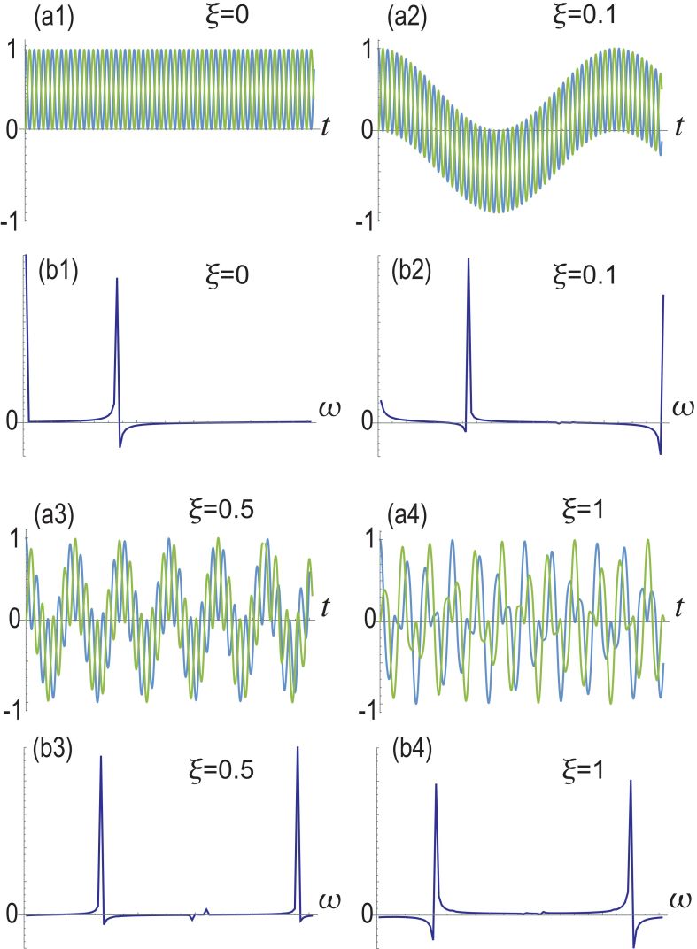
Figure 4: (a1)$\sim$(a4) Time evolution of Re[$\psi_{1}(t)$] in the nonlinear Schrödinger model on the dimer described by Eqs.(35) and (36). (a1), (b1) $\xi=0$; (a2), (b2) $\xi=0.1$; (a3), (b3) $\xi=0.5$; (a4), (b4) $\xi=1$. (a1)$\sim$(a4) The vertical axis is Re[$\psi_{1}(t)$] and the horizontal axis is the time $t$. (b1)$\sim$(b4) Fourier component of Re[$\psi_{1}(\omega)$]. The horizontal axis is the frequency $\omega$, which is the Fourier component of the time $t$, while the vertical axis is Re[$\psi_{1}(\omega)$].

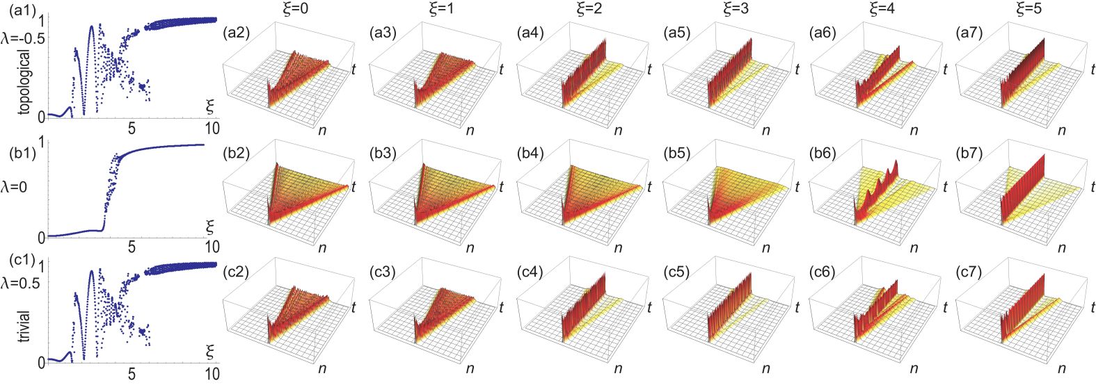
Figure 5: (a1)$\sim$(c1) Amplitude $|\psi_{1}|$ after enough time as a function of $\xi$. (a2)$\sim$(a7), (b2)$\sim$(b7) and (c2)$\sim$(c7) Time evolution of $|\psi_{n}|$ in the discrete nonlinear Schrödinger equation (2). (a1)$\sim$(a7) topological phase at $\lambda=-0.5$, (a1)$\sim$(a7) topological phase boundary at $\lambda=0$, and (a1)$\sim$(a7) trivial phase at $\lambda=0.5$.

III.2 Phase diagram

Starting from the initial condition (16), we explore the time evolution of $\psi_{n}$ for various $\xi$ and show the results in Fig.2(b). As indicated by a general consideration given before, we find that there remains a finite component at the edge site ($n=1$) in the topological phase, while it is almost zero in the trivial phase.

We show the absolute value of $\psi_{1}$ after enough time as a function of $\lambda$ for various $\xi$ in Fig.3(b1)$\sim$(b4). First, we study the linear model as shown in Fig.3(b1). The amplitude $\left|\psi_{1}\right|$ is finite in the topological phase, while it is almost zero in the trivial phase. The overall structure is almost identical in the linear limit ($\xi=0$) and in the weak nonlinear regime ($\xi=0.1$) as shown in Fig.3(b2). For medium nonlinearity ($\xi=1$), there appears an oscillation mode for $\lambda\geq 0.55$, as shown in Fig.3(b3). We will argue that this is due to the dimerization effect in Sec.III.4. For strong nonlinearity ($\xi=5$), the amplitude $\left|\psi_{1}\right|$ is almost 1 for $\lambda\leq 0.52$. We have already argued that this is due to the nonlinearity-induced localization in Sec.II.3.

There are four phases. First, we have the topological and trivial phases in the weak nonlinear regime. The topological phase boundary is almost independent of the nonlinearity $\xi$ . The amplitude gradually decreases from $1$ to $0$ depending on the dimerization from $\lambda=-1$ to $\lambda=0$, as we have argued in Sec.II.2. On the other hand, there is a nonlinearity-induced localization phase for large $\xi$. The amplitude is almost $1$ entirely in the nonlinearity-induced localization phase, as we have argued in Sec.II.3.

In addition, there is a dimer phase in the vicinity of $\lambda\simeq 1$, where the system is almost dimerized. The states $\psi_{1}$ and $\psi_{2}$ oscillate between the two adjacent sites ($n=1,2$) at the edge. Furthermore, the trivial phase penetrates into the dimer phase for $\lambda\geq 0.25$ in Fig.3(a2) as in (a3).

III.3 Topological number

The hopping matrix (29) leads to the SSH Hamiltonian in the momentum space,

$$M\left(k\right)=-\left(t_{A}+t_{B}\right)I_{2}+\left(\begin{array}[]{cc}0&t_{A}+t_{B}e^{-ik}\\ t_{A}+t_{B}e^{ik}&0\end{array}\right).$$ (33)

The topological number is the Berry phase defined by

$$p_{i}=\frac{1}{2\pi}\int_{9}^{2\pi}A\left(k\right)dk,$$ (34)

where $A\left(k\right)=-i\left\langle\psi(k)\right|\partial_{k}\left|\psi(k)\right\rangle$ is the Berry connection with $\psi(k)$ the eigenfunction of $M\left(k\right)$. We obtain $\Gamma=1$ for $\lambda<0$ and $\Gamma=0$ for $\lambda>0$. It is known that the SSH system is topological for $\lambda<0$ and trivial for $\lambda>0$. There are two isolated edge states in the limit $\lambda\simeq-1$, while all of the states are dimerized in the limit $\lambda\simeq 1$: See Fig.1(a).

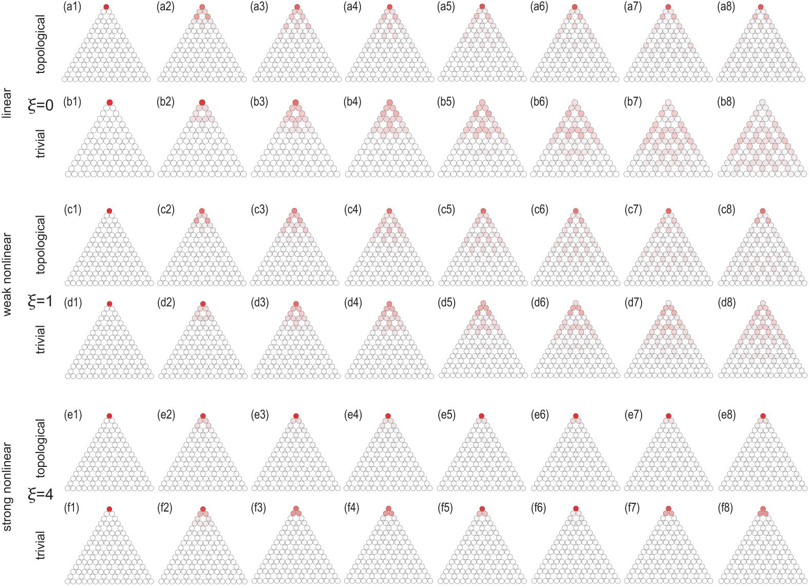
Figure 6: Time evolution of the spatial distribution of the amplitude $|\psi_{n}|$ in the nonlinear breathing Kagome model. (a1)$\sim$(b8) linear model with $\xi=0$ for various time. (c1)$\sim$(d8) weak nonlinear model with $\xi=1$. (e1)$\sim$(f8) strong nonlinear model with $\xi=4$, where the system is in the nonlinearity-induced localized phase. The color density indicates the amplitude $|\psi_{n}|$ . We have set $\lambda=-0.5$ for (a1)$\sim$(a8), (c1)$\sim$(c8) and (e1)$\sim$(e8), where the system is topological, while we have set $\lambda=0.5$ for (b1)$\sim$(b8), (d1)$\sim$(d8) and (f1)$\sim$(f8), where the system is trivial.

III.4 Dimer limit

Next, we study the dimer limit with $t_{B}=0$ as in Fig.1(a3), where $\lambda=1$. The differential equations are explicitly given by

$$i\frac{d\psi_{1}}{dt} =t_{A}\left(\psi_{2}-\psi_{1}\right)-\xi\left|\psi_{1}\right|^{2}\psi_{1},$$ (35)

$$i\frac{d\psi_{2}}{dt} =t_{A}\left(\psi_{1}-\psi_{2}\right)-\xi\left|\psi_{2}\right|^{2}\psi_{2}.$$ (36)

We show a numerical solution of the time evolution of $\psi_{1}$ and $\psi_{2}$ in Fig.4.

In the linear model ($\xi=0$), they oscillate alternately without changing their amplitudes,

$$\psi_{1}=e^{-it_{A}t}\cos t_{A}t,\qquad\psi_{2}=ie^{-it_{A}t}\sin t_{A}t,$$ (37)

where the phases are different by $\pi$. Once the nonlinearity is introduced, there appears an oscillation whose period is much longer than the original period. The overall oscillation period becomes shorter as the nonlinearity increases. It shows a complicated behavior for strong nonlinearity as in Fig.4.

In the nonlinear model ($\xi\neq 0$), there is an oscillatory behavior with long and short periods in the dimer phase as in Fig.4. This is easily seen by examining the Fourier component $\psi\left(\omega\right)$, where $\omega$ is the frequency as in Fig.4(b1)$\sim$(b4). There are two sharp peaks in $\psi\left(\omega\right)$, which indicates that there are short-period and long-period modes.

This oscillatory behavior may be understood as follows. By using an ansatz

$$\psi_{2}=-\psi_{1},$$ (38)

the equations (35) and (36) are summarized to one equation

$$i\frac{d\psi_{1}}{dt}=-2t_{A}\psi_{1}-\xi\left|\psi_{1}\right|^{2}\psi_{1},$$ (39)

whose solution is given by

$$\theta_{1}=\left(2t_{A}+\xi r_{n}^{2}\right)t+c,$$ (40)

and a constant $r_{1}$ with the polar expression (23). This explains a short-period oscillation mode in Fig.4.

However, the ansatz (38) for the analytical solution is not compatible to the initial condition (7). Thus, we cannot apply the analytic solution (40) for the quench dynamics, although the ansatz (38) holds after enough time. In order to adjust the ansatz (38) to the initial condition (7), the long-period oscillation mode would appear.

These dimer oscillations give rise to the dimer phase in the vicinity of $\lambda=1$ in the phase diagram in Fig.3(a3).

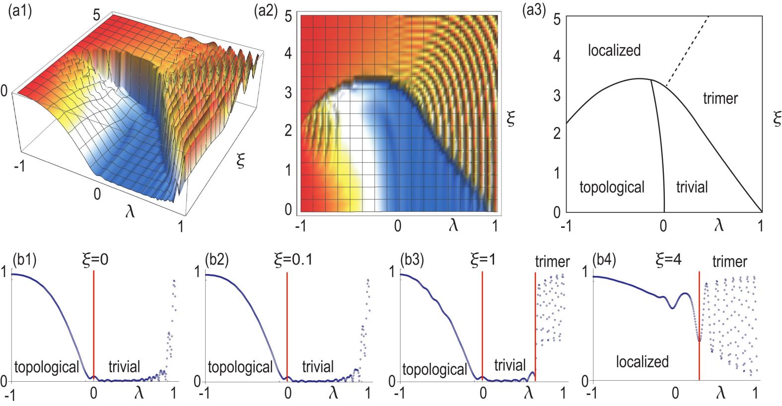
Figure 7: (a1)$\sim$(a3) Phase diagram of the nonlinear breathing Kagome model. (a1) Bird’s eye’s view, (a2) top view, and (a3) schematic illustration of the phase diagram. (b1)$\sim$(b4) Amplitude $|\psi_{1}|$ as a function of $\lambda$ for various $\xi$. (b1) $\xi=0$, (b2) $\xi=0.1$, (b3) $\xi=1$, and (b4) $\xi=5$.

III.5 Discrete nonlinear Schrödinger equation

The discrete nonlinear Schrödinger equation (2) is a limit of the nonlinear SSH model (30) and (31) by setting $\lambda=0$. We show the time evolution of $\psi_{n}$ starting from the initial condition (7), where the initial state is taken at the site $m$ in the bulk in Fig.5. For weak nonlinearity $\xi\lesssim 4$, the state rapidly spreads as shown in Fig.5(b2)$\sim$(b7). On the other hand, for strong nonlinearity $\xi\gtrsim 4$, the state almost remains at the initial site $m$ as shown in Fig.5(b6) and (b7). We also show $\left|\psi_{1}\right|$ as a function of $\xi$ in Fig.5(b1). It shows a drastic change at $\xi\simeq 4$ for $\lambda=0$, which indicates the nonlinearity-induced localization transition.

We have also shown the time evolution of $\psi_{n}$ starting from the initial condition (7) in the case of the nonlinear SSH model in Fig5(a2)$\sim$(a7) for the topological phase with $\lambda=-0.5$ and Fig5(c2)$\sim$(c7) for the trivial phase with $\lambda=0.5$. The nonlinearity-induced localization transition is found to occur at $\xi\simeq 2$.

It is to be noted in Fig5 that there is almost no difference in the dynamics of $\left|\psi_{n}\right|$ between the topological and trivial phases for $\lambda=\mp 0.5$. It dictates that we cannot differentiate the topological and trivial phases by starting from a site in the bulk. It is because the bulk state is almost identical between the topological and trivial phases. The key difference is the presence of topological edge or corner states in the topological phase.

As a result, the nonlinearity-induced localization occurs irrespective of the dimerization $\lambda$. It is because the nonlinearity effect is dominant in the dynamics for large $\xi$.

IV Nonlinear second-order topological phases

IV.1 Model

Recently, the nonlinear second-order topological phase has been studied in photonicsKirch . We proceed to study the case where the matrix $M_{nm}$ describes the breathing Kagome lattice, whose lattice structure is illustrated in Fig.1(b). The matrix $M$ in the momentum space is given byEzawaKagome

$$M\left(\mathbf{k}\right)=-\left(\begin{array}[]{ccc}0&h_{12}&h_{13}\\ h_{12}^{\ast}&0&h_{23}\\ h_{13}^{\ast}&h_{23}^{\ast}&0\end{array}\right),$$ (41)

with

$$h_{12} =t_{A}e^{i\left(k_{x}/2+\sqrt{3}k_{y}/2\right)}+t_{B}e^{-i\left(k_{x}/2+\sqrt{3}k_{y}/2\right)},$$ (42)

$$h_{23} =t_{A}e^{i\left(k_{x}/2-\sqrt{3}k_{y}/2\right)}+t_{B}e^{i\left(-k_{x}/2+\sqrt{3}k_{y}/2\right)},$$ (43)

$$h_{13} =t_{A}e^{ik_{x}}+t_{B}e^{-ik_{x}},$$ (44)

where we have introduced two hopping parameters $t_{A}$ and $t_{B}$ corresponding to upward and downward triangles, as shown in Fig.1(b).

IV.2 Topological number

There are three mirror symmetries for the breathing Kagome lattice. They are the mirror symmetries $M_{x}$ with respect to the $x$ axis, and $M_{\pm}$ with respect to the two lines obtained by rotating the $x$ axis by $\pm 2\pi/3$. The polarization along the $x_{i}$ axis is the expectation value of the position,

$$p_{i}=\frac{1}{S}\int_{\text{BZ}}A_{i}d^{2}\mathbf{k},$$ (45)

where $A_{i}=-i\left\langle\psi(\mathbf{k})\right|\partial_{k_{i}}\left|\psi(\mathbf{k})\right\rangle$ is the Berry connection with $x_{i}=x,y$, and $S=8\pi^{2}/\sqrt{3}$ is the area of the Brillouin zone; $\psi(\mathbf{k})$ the eigenfunction of $M\left(\mathbf{k}\right)$.

The topological number is defined byEzawaKagome

$$\Gamma=3\left(p_{x}^{2}+p_{y}^{2}\right).$$ (46)

We obtain $\Gamma=0$ for $t_{A}/t_{B}<-1$ and $t_{A}/t_{B}>2$, which is the trivial phase with no zero-mode corner states. On the other hand, we obtain $\Gamma=1$ for $-1<t_{a}/t_{b}<1/2$, which is the topological phase with the emergence of three zero-mode corner states. Finally, $\Gamma$ is not quantized for $1/2<t_{A}/t_{B}<2$, which is the metallic phase.

For $t_{A}=0$, three corner sites are perfectly decoupled from the bulk as in Fig.1(b1). On the other hand, for $t_{B}=0$, all sites are trimerized as in Fig.1(b3). We study a quench dynamics starting from the initial condition (16), where the state is perfectly localized at the top corner site. We note that we use the tight-bind model although the continuum model is used in the previous workKirch , where the essential physics is identical.

IV.3 Phase diagram

We show the phase diagram in Fig.7. There are four phases in the nonlinear breathing Kagome model. The trimer phase appears instead of the dimer phase characteristic to the nonlinear SSH model. The trimer phase and the nonlinearity-induced localization phase are smoothly connected, both of which are irrelevant to the topological number. The difference is that there is an oscillatory behavior in the trimer phase but not in the nonlinearity-induced localization phase. On the other hand, there is a sharp transition between the trivial and nonlinearity-induced localization phases. This is also the case for the transition between the trivial and trimer phase. As in the case of the nonlinear SSH model, the topological phase boundary between the topological and trivial phases is almost unchanged for $0\leq\xi\lesssim 3$ as in Fig.7(a3).

We start with the study of the linear model ($\xi=0$). We show the spatial distribution of the amplitude $|\psi_{n}|$ for various time in Fig.6(a1)$\sim$(a8) and Fig.6(b1)$\sim$(b8). In the topological phase, the amplitude remains finite at the top corner site. On the other hand, the amplitude rapidly spreads into the bulk and disappears in the trivial phase.

The weak nonlinear regime ($\xi\simeq 0$) is analyzed just as in Sec.II.2. Namely, the topological analysis based on the formula (20) is valid as in the linear model. We have numerically confirmed this observation in Fig.6(c1)$\sim$(c8). Indeed, we may regard the system even with $\xi=1$ as the one in the weak nonlinear regime. We show the spatial distribution for $\xi=1$ in Fig.6(c1)$\sim$(c8), which is almost identical to the one in the linearized model ($\xi=0$) in Fig.6(a1)$\sim$(a8). This is also the case for the trivial phase as shown in Fig.6(d1)$\sim$(d8). The amplitude at the top corner site after enough time is shown in Fig.7(b1)$\sim$(b4). We note that the overall feature is quite similar to the one in the nonlinear SSH model. On the other hand, the state is localized in both of the topological and trivial phases for $\xi=4$ in Fig.6(e1)$\sim$(e8) and Fig.6(f1)$\sim$(f8). It indicates that the state is in the nonlinearity-induced localization phase.

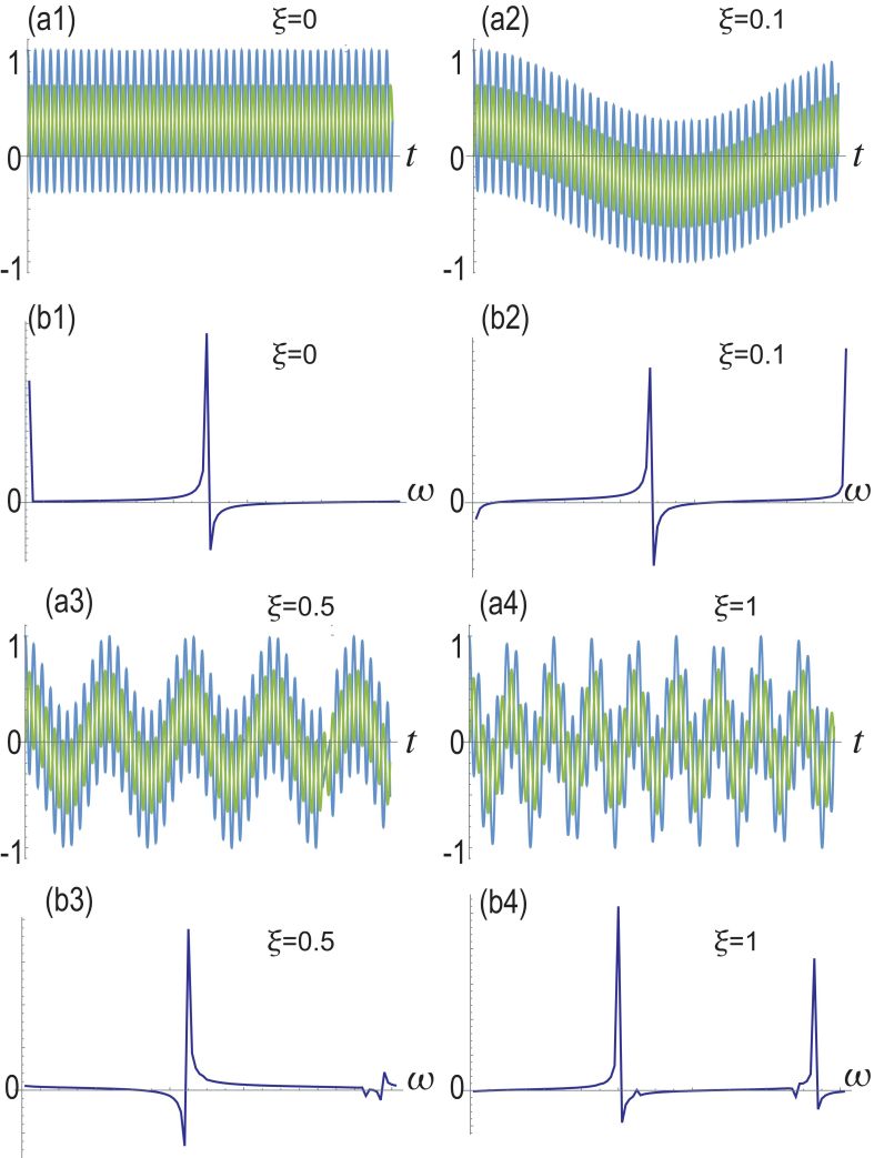
Figure 8: (a1)$\sim$(a4) Time evolution of Re[$\psi_{1}(t)$] in the nonlinear Schrödinger model on the trimer described by Eqs.(47), (48) and (49). (a1), (b1) $\xi=0$; (a2), (b2) $\xi=0.1$; (a3), (b3) $\xi=0.5$; (a4), (b4) $\xi=1$. (a1)$\sim$(a4) The vertical axis is Re[$\psi_{1}(t)$] and the horizontal axis is time. (b1)$\sim$(b4) Fourier component of Re[$\psi_{1}(\omega)$]. The horizontal axis is the frequency $\omega$, which is the Fourier component of the time $t$, while the vertical axis is Re[$\psi_{1}(\omega)$].

IV.4 Trimer limit

Next, we study the trimer limit with $t_{B}=0$ as in Fig.1(b3), where $\lambda=1$. The differential equations are explicitly given by

$$i\frac{d\psi_{1}}{dt} =\varepsilon\psi_{1}+t_{A}\left(\psi_{1}-\psi_{2}\right)+t_{A}\left(\psi_{1}-\psi_{3}\right)-\xi\left|\psi_{1}\right|^{2}\psi_{1},$$ (47)

$$i\frac{d\psi_{2}}{dt} =\varepsilon\psi_{2}+t_{A}\left(\psi_{2}-\psi_{1}\right)+t_{A}\left(\psi_{2}-\psi_{3}\right)-\xi\left|\psi_{2}\right|^{2}\psi_{2},$$ (48)

$$i\frac{d\psi_{3}}{dt} =\varepsilon\psi_{3}+t_{A}\left(\psi_{3}-\psi_{1}\right)+t_{A}\left(\psi_{3}-\psi_{2}\right)-\xi\left|\psi_{3}\right|^{2}\psi_{3}.$$ (49)

Without loss of generality we may set $\psi_{2}=\psi_{3}$ and obtain

$$i\frac{d\psi_{1}}{dt} =\varepsilon\psi_{1}+2t_{A}\left(\psi_{1}-\psi_{2}\right)-\xi\left|\psi_{1}\right|^{2}\psi_{1},$$ (50)

$$i\frac{d\psi_{2}}{dt} =\varepsilon\psi_{2}+t_{A}\left(\psi_{2}-\psi_{1}\right)-\xi\left|\psi_{2}\right|^{2}\psi_{2}.$$ (51)

It is hard to solve these equations analytically except for the linear model, where the solution is given by

$$\psi_{1} =\frac{1}{3}\left(1+2e^{-3it_{A}t}\right),$$ (52)

$$\psi_{2} =\psi_{3}=\frac{1}{3}\left(1-e^{-3it_{A}t}\right).$$ (53)

Although this is modified smoothly as a function of $\xi$, it presents the short-period oscillation. The long-period oscillation emerges once the nonlinearity $\xi$ is introduced. We show the Fourier component $\psi\left(\omega\right)$ in Fig.8(b1)-(b4), where we see two sharp peaks in $\psi\left(\omega\right)$ corresponding to the short-period and long-period oscillations.

These trimer oscillations give rise to the trimer phase in the vicinity of $\lambda=1$ in the phase diagram in Fig.7(a3).

V Conclusion

The topological physics has been developed in linear systems such as condensed matter systems, electric circuits and acoustic systems. The key issue of the topological physics is the emergence of topological edge or corner states in the topological phase, which has been firmly established by various experimental observation. Now there are attempts generalize it to nonlinear systems.

In the present work, we investigated the one-dimensional nonlinear SSH model and the two-dimensional nonlinear breathing Kagome model. These models contain the hopping term $\sum_{m}M_{nm}\psi_{m}$ and the nonlinear term $\xi\left|\psi_{n}\right|^{2}\psi_{n}$. Dynamics is determined as a result of the competition between these two terms. As far as the hopping term is dominant, the topological dynamics is valid in these models. On the other hand, when the nonlinear term is dominant, the nonlinearity-induced localization phase emerges. There is another phenomenon due to a cooperative effect of these two terms, which is the oscillation mode in the dimer (trimer) limit of the nonlinear SSH (breathing Kagome) model. We have studied these new phenomena analytically and numerically. Our results are summarized in the phase diagrams in Fig.3 and in Fig.7.

These results show that there are varieties of the effect of nonlinearity to topological phases. It is an interesting problem to study various nonlinear topological systems.

The author is very much grateful to N. Nagaosa for helpful discussions on the subject. This work is supported by the Grants-in-Aid for Scientific Research from MEXT KAKENHI (Grants No. JP17K05490 and No. JP18H03676). This work is also supported by CREST, JST (JPMJCR16F1 and JPMJCR20T2).

References

- (1) M. Z. Hasan and C. L. Kane, Rev. Mod. Phys. 82, 3045 (2010).
- (2) X.-L. Qi and S.-C. Zhang, Rev. Mod. Phys. 83, 1057 (2011).
- (3) F. Zhang, C.L. Kane and E.J. Mele, Phys. Rev. Lett. 110, 046404 (2013).
- (4) W. A. Benalcazar, B. A. Bernevig, and T. L. Hughes, 10.1126/science.aah6442.
- (5) F. Schindler, A. Cook, M. G. Vergniory, and T. Neupert, in APS March Meeting (2017).
- (6) Y. Peng, Y. Bao, and F. von Oppen, Phys. Rev. B 95, 235143 (2017).
- (7) J. Langbehn, Y. Peng, L. Trifunovic, F. von Oppen, and P. W. Brouwer, Phys. Rev. Lett. 119, 246401 (2017).
- (8) Z. Song, Z. Fang, and C. Fang, Phys. Rev. Lett. 119, 246402 (2017).
- (9) W. A. Benalcazar, B. A. Bernevig, and T. L. Hughes, Phys. Rev. B 96, 245115 (2017).
- (10) F. Schindler, A. M. Cook, M. G. Vergniory, Z. Wang, S. S. P. Parkin, B. A. Bernevig, and T. Neupert, Science Advances 4, eaat0346 (2018).
- (11) C. Fang, L. Fu, arXiv:1709.01929.
- (12) M. Ezawa, Phys. Rev. Lett. 120, 026801 (2018).
- (13) E. Khalaf, H. C. Po, A. Vishwanath and H. Watanabe, Phys. Rev. X 8, 031070 (2018).
- (14) A. B. Khanikaev, S. H. Mousavi, W.-K. Tse, M. Kargarian, A. H. MacDonald, G. Shvets, Nature Materials 12, 233 (2013).
- (15) M. Hafezi, E. Demler, M. Lukin, J. Taylor, Nature Physics 7, 907 (2011).
- (16) M. Hafezi, S. Mittal, J. Fan, A. Migdall, J. Taylor, Nature Photonics 7, 1001 (2013).
- (17) L.H. Wu and X. Hu, Phys. Rev. Lett. 114, 223901 (2015).
- (18) L. Lu. J. D. Joannopoulos and M. Soljacic, Nature Photonics 8, 821 (2014).
- (19) T. Ozawa, H. M. Price, N. Goldman, O. Zilberberg and I. Carusotto Phys. Rev. A 93, 043827 (2016).
- (20) D. Leykam and Y. D. Chong, Phys. Rev. Lett. 117, 143901 (2016).
- (21) A. B. Khanikaev and G. Shvets, Nature Photonics 11, 763 (2017).
- (22) X. Zhou, Y. Wang, D. Leykam and Y. D. Chong, New J. Phys. 19, 095002 (2017).
- (23) P. St-Jean, V. Goblot, E. Galopin, A. Lemaitre, T. Ozawa, L. Le Gratiet, I. Sagnes, J. Bloch and A. Amo, Nature Photonics 11, 651 (2017).
- (24) Y. Ota, R. Katsumi, K. Watanabe, S. Iwamoto and Y. Arakawa, Communications Physics 1, 86 (2018)
- (25) T. Ozawa, H. M. Price, A. Amo, N. Goldman, M. Hafezi, L. Lu, M. C. Rechtsman, D. Schuster, J. Simon, O. Zilberberg and L. Carusotto, Rev. Mod. Phys. 91, 015006 (2019).
- (26) Y. Ota, F. Liu, R. Katsumi, K. Watanabe, K. Wakabayashi, Y. Arakawa and S. Iwamoto, Optica 6, 786 (2019).
- (27) T. Ozawa and H. M. Price, Nature Reviews Physics 1, 349 (2019).
- (28) A. E. Hassan, F. K. Kunst, A. Moritz, G. Andler, E. J. Bergholtz, M. Bourennane, Nature Photonics 13, 697 (2019).
- (29) Y. Ota, K. Takata, T. Ozawa, A. Amo, Z. Jia, B. Kante, M. Notomi, Y. Arakawa, S.i Iwamoto, Nanophotonics 9, 547 (2020).
- (30) M. Li, D. Zhirihin, D. Filonov, X. Ni, A. Slobozhanyuk, A. Alu and A. B. Khanikaev, Nature Photonics 14, 89 (2020).
- (31) H. Yoshimi, T. Yamaguchi, Y. Ota, Y. Arakawa and S. Iwamoto, Optics Letters 45, 2648 (2020).
- (32) M. Kim, Z. Jacob and J. Rho, Light: Science and Applications 9, 130 (2020).
- (33) S. Iwamoto, Y. Ota and Y. Arakawa, Optical Materials Express 11, 319 (2021).
- (34) E. Prodan and C. Prodan, Phys. Rev. Lett. 103, 248101 (2009).
- (35) Z. Yang, F. Gao, X. Shi, X. Lin, Z. Gao, Y. Chong and B. Zhang, Phys. Rev. Lett. 114, 114301 (2015).
- (36) P. Wang, L. Lu and K. Bertoldi, Phys. Rev. Lett. 115, 104302 (2015).
- (37) M. Xiao, G. Ma, Z. Yang, P. Sheng, Z. Q. Zhang and C. T. Chan, Nat. Phys. 11, 240 (2015).
- (38) C. He, X. Ni, H. Ge, X.-C. Sun,Y.-B. Chen1 M.-H. Lu, X.-P. Liu, L. Feng and Y.-F. Chen, Nature Physics 12, 1124 (2016).
- (39) H. Abbaszadeh, A. Souslov, J. Paulose, H. Schomerus and V. Vitelli, Phys. Rev. Lett. 119, 195502 (2017).
- (40) H. Xue, Y. Yang, F. Gao, Y. Chong and B.Zhang, Nature Materials 18, 108 (2019).
- (41) X. Ni, M. Weiner, A. Alu and A. B. Khanikaev, Nature Materials 18, 113 (2019).
- (42) M. Weiner, X. Ni, M. Li, A. Alu, A. B. Khanikaev, Science Advances 6, eaay4166 (2020).
- (43) H. Xue, Y. Yang, G. Liu, F. Gao, Y. Chong and B. Zhang, Phys. Rev. Lett. 122, 244301 (2019).
- (44) C. L. Kane and T. C. Lubensky, Nature Phys. 10, 39 (2014).
- (45) B. Gin-ge Chen, N. Upadhyaya and V. Vitelli, PNAS 111, 13004 (2014).
- (46) L. M. Nash, D. Kleckner, A. Read, V. Vitelli, A. M. Turner and W. T. M. Irvine, PNAS 112, 14495 (2015).
- (47) J. Paulose, A. S. Meeussen and V. Vitelli, PNAS 112, 7639 (2015).
- (48) R. Susstrunk, S. D. Huber, Science 349, 47 (2015).
- (49) R. Susstrunk and S. D. Huber, Proc. Natl. Acad. Sci. USA 113, E4767 (2016).
- (50) S. D. Huber, Nature Physics 12, 621 (2016).
- (51) A. S. Meeussen, J. Paulose and V. Vitelli, Phys. Rev. X 6, 041029 (2016).
- (52) T. Kariyado and Y. Hatsugai, Sci. Rep. 5, 18107 (2016).
- (53) T. Kariyado and Y. Hatsugai, J. Phys. Soc. Jpn. 85, 043001 (2016).
- (54) H. C. Po, Y. Bahri and A. Vishwanath, Phys. Rev. B 93, 205158 (2016).
- (55) D. Zeb Rocklin, Bryan Gin–ge Chen, Martin Falk, Vincenzo Vitelli, and T. C. Lubensky, Phys. Rev. Lett. 116, 135503 (2016).
- (56) Y. Takahashi, T. Kariyado and Y. Hatsugai, New J. Phys. 19, 035003 (2017).
- (57) K. H. Matlack, M. Serra-Garcia, A. Palermo, S. D. Huber and C. Daraio, Nature Mat. 17, 323 (2018).
- (58) Y. Takahashi, T. Kariyado and Y. Hatsugai, Phys. Rev. B 99, 024102 (2019).
- (59) A. Ghatak, M. Brandenbourger, J. van Wezel and C. Coulais, Proc. Natl. Ac. Sc. U.S.A. 117, 29561 (2020).
- (60) H. Wakao, T. Yoshida, H. Araki, T. Mizoguchi and Y. Hatsugai, Phys. Rev. B 101, 094107 (2020).
- (61) S. Imhof, C. Berger, F. Bayer, J. Brehm, L. Molenkamp, T. Kiessling, F. Schindler, C. H. Lee, M. Greiter, T. Neupert, R. Thomale, Nat. Phys. 14, 925 (2018).
- (62) C. H. Lee , S. Imhof, C. Berger, F. Bayer, J. Brehm, L. W. Molenkamp, T. Kiessling and R. Thomale, Communications Physics, 1, 39 (2018).
- (63) T. Helbig, T. Hofmann, C. H. Lee, R. Thomale, S. Imhof, L. W. Molenkamp and T. Kiessling, Phys. Rev. B 99, 161114 (2019).
- (64) Y. Lu, N. Jia, L. Su, C. Owens, G. Juzeliunas, D. I. Schuster and J. Simon, Phys. Rev. B 99, 020302 (2019).
- (65) Y. Li, Y. Sun, W. Zhu, Z. Guo, J. Jiang, T. Kariyado, H. Chen and X. Hu, Nat. Com. 9, 4598 (2018).
- (66) M. Ezawa, Phys. Rev. B 98, 201402(R) (2018).
- (67) K. Luo, R. Yu and H. Weng, Research, ID 6793752. (2018).
- (68) E. Zhao, Ann. Phys. 399, 289 (2018).
- (69) M. Ezawa, Phys. Rev. B 99, 201411(R) (2019).
- (70) M. Ezawa, Phys. Rev. B 99, 121411(R) (2019).
- (71) M. Serra-Garcia, R. Susstrunk and S. D. Huber, Phys. Rev. B 99, 020304 (2019).
- (72) T. Hofmann, T. Helbig, C. H. Lee, M. Greiter, R. Thomale, Phys. Rev. Lett. 122, 247702 (2019).
- (73) M. Ezawa, Phys. Rev. B 100, 045407 (2019).
- (74) M. Ezawa, Phys. Rev. B 102, 075424 (2020).
- (75) C. H. Lee, T. Hofmann, T. Helbig, Y. Liu, X. Zhang, M. Greiter and R. Thomale, Nature Communications 11, 4385 (2020).
- (76) T. Kotwal, H. Ronellenfitsch, F. Moseley, A. Stegmaier, R. Thomale, J. Dunkel, PNAS 118, e2106411118 (2021).
- (77) D. Smirnova, D. Leykam, Y. Chong and Y. Kivshar, Applied Physics Reviews 7, 021306 (2020).
- (78) S. Kruk, A. Poddubny, D. Smirnova, L. Wang, A. Slobozhanyuk, A. Shorokhov, I. Kravchenko, B. Luther-Davies and Y. Kivshar, Nature Nanotechnology 14, 126 (2019).
- (79) Lukas J. Maczewsky, Matthias Heinrich, Mark Kremer, Sergey K. Ivanov, Max Ehrhardt, Franklin Martinez, Yaroslav V. Kartashov, Vladimir V. Konotop, Lluis Torner, Dieter Bauer, Alexander Szameit, Science 370, 701 (2010).
- (80) F. Zangeneh-Nejad and R. Fleury, Phys. Rev. Lett. 123, 053902 (2019).
- (81) M. S. Kirsch, Y. Zhang, M. Kremer, L. J. Maczewsky, S. K. Ivanov, Y. V. Kartashov, L. Torner, D. Bauer, A. Szameit and M. Heinrich, Nature Physics 17, 995 (2021).
- (82) M. Ezawa, cond-mat/arXiv:2105.10851
- (83) M. Ezawa, arXiv:2108.09634.
- (84) A. Szameit, D. Blöer, J. Burghoff, T. Schreiber, T. Pertsch, S. Nolte, A. Tünnermann and F. Lederer, Optics Express 13, 10552 (2005).
- (85) D. N. Christodoulides, F. Lederer and Y. Silberberg, Nature 424, 817 (2003)
- (86) D. Cai, A. R. Bishop and N. Gronbech-Jensen, Phys. Rev. Lett. 72, 591 (1994).
- (87) P. G. Kevrekidis, K. O. Rasmussen and A. R. Bishop, Int. J. Mod. Phys. B 15, 2833 (2001).
- (88) J. C. Eilbeck, P. S. Lomdahl and A. C. Scott, Physica D 16, 318, (1985).
- (89) N. Korabel and G. M. Zaslavsky, Physica A: Statistical Mechanics and its Applications, 378, 223 (2006).
- (90) Y. Hadad, J. C. Soric, A. B. Khanikaev, and A. Alù, Nature Electronics 1, 178 (2018).
- (91) M. A. Gorlach, A. P. Slobozhanyuk, Nanosystems: Physics, Cheminstry, Mathematics, 8, 695 (2017).
- (92) T. Tuloup, R. W. Bomantara, C. H. Lee and J. Gong, Phys. Rev. B 102, 115411 (2020).