\jmlrvolume\jmlryear\jmlrproceedings

Infinitely Divisible Noise in the Low Privacy Regime

\NameRasmus Pagh \Emailpagh@di.ku.dk
\addrBARC and University of Copenhagen
   \NameNina Mesing Stausholm \Emailnimn@itu.dk
\addrIT University of Copenhagen
Abstract

Federated learning, in which training data is distributed among users and never shared, has emerged as a popular approach to privacy-preserving machine learning. Cryptographic techniques such as secure aggregation are used to aggregate contributions, like a model update, from all users. A robust technique for making such aggregates differentially private is to exploit infinite divisibility of the Laplace distribution, namely, that a Laplace distribution can be expressed as a sum of i.i.d. noise shares from a Gamma distribution, one share added by each user.

However, Laplace noise is known to have suboptimal error in the low privacy regime for ε𝜀\varepsilon-differential privacy, where ε>1𝜀1\varepsilon>1 is a large constant. In this paper we present the first infinitely divisible noise distribution for real-valued data that achieves ε𝜀\varepsilon-differential privacy and has expected error that decreases exponentially with ε𝜀\varepsilon.

keywords:
Differential privacy, federated learning.

1 Introduction

Differential privacy, a state-of-the-art privacy definition, is a formal constraint on randomized mechanisms for privately releasing results of computations. It gives a formal framework for quantifying how well the privacy of an individual, whose data is part of the input, is preserved. In recent years, differentially private algorithms for machine learning have been developed and made available, for example, in TensorFlow/privacy and the Opacus library for PyTorch. Using such algorithms ensures that the presence or absence of a single data record in a database does not significantly affect the distribution of the model produced.

Concurrently, the area of federated learning (McMahan et al., 2017) has explored how to carry out machine learning in settings where training data is distributed among n𝑛n users and never shared. Cryptographic techniques such as secure aggregation are used to aggregate contributions, like a model update, from all users (Bonawitz et al., 2017). This setup is used, for example, in the federated learning system run by Google on data from Android phones.***https://ai.googleblog.com/2017/04/federated-learning-collaborative.html A robust technique for making such aggregates differentially private is to exploit infinite divisibility of the Laplace distribution, namely, that a Laplace distribution can be expressed as a sum of n𝑛n i.i.d. noise shares from a Gamma distribution, one share added to the input of each user (Goryczka and Xiong, 2017). That is, if user i𝑖i holds xi[0,Δ]subscript𝑥𝑖0Δx_{i}\in[0,\Delta], the input provided to the secure aggregation is xi+ηisubscript𝑥𝑖subscript𝜂𝑖x_{i}+\eta_{i}, where ηisubscript𝜂𝑖\eta_{i} is sampled from a suitable Gamma distribution. Infinitely divisible noise is resistent to dropout, where some users never contribute to the sum, if we set n𝑛n to be a lower bound on the number of fully participating users.

However, the Laplace noise needed for ε𝜀\varepsilon-differential privacy yields expected error Θ(Δ/ε)ΘΔ𝜀\Theta(\Delta/\varepsilon), which is not optimal in the “low privacy regime” when ε1much-greater-than𝜀1\varepsilon\gg 1. Geng, Kairouz, Oh, and Viswanath (2015) and Geng and Viswanath (2016a) presented the Staircase mechanism (see Lemma B.7), which can be parameterized to obtain expected error Θ(Δeε/2)ΘΔsuperscript𝑒𝜀2\Theta(\Delta e^{-\varepsilon/2}) or variance Θ(Δ2e2ε/3)ΘsuperscriptΔ2superscript𝑒2𝜀3\Theta(\Delta^{2}e^{-2\varepsilon/3}), thus outperforming the Laplace mechanism for ε𝜀\varepsilon larger than some constant. However, the noise distribution used by this mechanism is not infinitely divisible, so it cannot replace Laplace noise in federated settings.

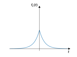
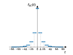
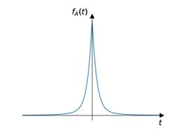
In this paper we present the first infinitely divisible noise distribution for real-valued data that achieves ε𝜀\varepsilon-differential privacy and has expected error that decreases exponentially with ε𝜀\varepsilon. Our new noise distribution, the Arete111The name Arete is inspired by the word arête (pronounced ”ah-ray’t”), which is a sharp-crested mountain ridge, while also a concept from Greek mythology, Arete (pronounced ”ah-reh-’tay”) referring to moral virtue and excellence: the notion of the fulfillment of purpose or function and the act of living up to one’s full potential (Wikipedia, ). distribution, has expected absolute value and variance exponentially decreasing in ε𝜀\varepsilon, and thus comparable to that of the Staircase distribution up to constant factors in ε𝜀\varepsilon. Figure 1 illustrates the shape of each of the three distributions.

\subfigure

[Laplace distribution] Refer to caption \subfigure[Staircase distribution] Refer to caption \subfigure[Arete distribution] Refer to caption

Figure 1: Illustration of the density functions for the Laplace, Staircase and Arete distributions.

The Arete distribution has a continuous density function implying that the privacy level decreases more smoothly with sensitivity, in contrast to the Staircase distribution (see discussion in Section 2).

The main part of this paper is devoted to the accuracy and privacy analysis of the Arete mechanism. Appendix A discusses applications in distributed private data analysis.

The Arete Distribution

For simplicity, we will limit ourselves to 1-dimensional setting. In order to deal with vectors (with subscript\ell_{\infty} sensitivity bounded by ΔΔ\Delta), we may simply add independent noise from the Arete distribution to each coordinate. Our goal is to approximate the staircase distribution with an infinitely divisible distribution, so it is instructive to understand the essential properties of the staircase distribution: Only probability mass exp(Ω(ε))Ω𝜀\exp({-\Omega(\varepsilon)}) is placed in the tails, which can be seen as a piece-wise uniform version of a scaled Laplace distribution. The majority of the probability mass is placed in a uniform distribution on an interval around zero of length exp(Ω(ε))Ω𝜀\exp({-\Omega(\varepsilon)}).

Definition 1.1 (Arete distribution, informal).

Let independent random variables X1,X2Γ(α,θ)similar-tosubscript𝑋1subscript𝑋2Γ𝛼𝜃X_{1},X_{2}\sim\Gamma(\alpha,\theta) and YLaplace(λ)similar-to𝑌𝐿𝑎𝑝𝑙𝑎𝑐𝑒𝜆Y\sim Laplace(\lambda). Then Z:=X1X2+Yassign𝑍subscript𝑋1subscript𝑋2𝑌Z:=X_{1}-X_{2}+Y has Arete distribution with parameters α,θ𝛼𝜃\alpha,\theta and λ𝜆\lambda, denoted Arete(α,θ,λ)𝐴𝑟𝑒𝑡𝑒𝛼𝜃𝜆Arete(\alpha,\theta,\lambda). When the parameters α𝛼\alpha, θ𝜃\theta and λ𝜆\lambda are understood from the context, we use fA(t)subscript𝑓𝐴𝑡f_{A}(t), t𝑡t\in\mathbb{R}, to denote the density function of Z𝑍Z.

Since the ΓΓ\Gamma and Laplace distributions are continuous and infinitely divisible, and the Laplace distribution is symmetric, it follows that the Arete distribution also has these properties. In Section 3.2 we show:

Lemma 1.2.

For any choice of parameters α,θ,λ>0𝛼𝜃𝜆0\alpha,\theta,\lambda>0, the Arete(α,θ,λ)𝐴𝑟𝑒𝑡𝑒𝛼𝜃𝜆Arete(\alpha,\theta,\lambda) distribution is infinitely divisible and has density fA(t)subscript𝑓𝐴𝑡f_{A}(t) that is continuous, symmetric around 0, and monotonely decreasing for t>0𝑡0t>0.

Next, we discuss the intuition behind the noise and privacy properties of the Arete distribution: For privacy parameter ε>0𝜀0\varepsilon>0 and sensitivity Δ>0Δ0\Delta>0 we concern ourselves with distributions 𝒟𝒟\mathcal{D} with support S𝑆S and density function f𝒟subscript𝑓𝒟f_{\mathcal{D}} satisfying

eεf𝒟(t)f𝒟(t+a)eε,t,a,|a|Δformulae-sequencesuperscript𝑒𝜀subscript𝑓𝒟𝑡subscript𝑓𝒟𝑡𝑎superscript𝑒𝜀for-all𝑡𝑎𝑎Δ\displaystyle e^{-\varepsilon}\leq\frac{f_{\mathcal{D}}(t)}{f_{\mathcal{D}}(t+a)}\leq e^{\varepsilon},\qquad\forall t,a\in\mathbb{R},|a|\leq\Delta (1)

as this property is sufficient to ensure differential privacy, which is our main goal. We will refer to the property (1) as the differential privacy constraint. In order to minimize the magnitude of the noise, the goal is to find a distribution with minimal expected (absolute) value while satisfying (1).

The difference of two ΓΓ\Gamma distributed random variables can be parameterized to have similar tails and to “peak” in an interval around zero of the same width as the staircase distribution. But this does not provide differential privacy since the density function has a singularity at zero. To achieve differential privacy we add a small amount of Laplace noise that “smooths out” the singularity. In more detail, the Γ(α,θ)Γ𝛼𝜃\Gamma(\alpha,\theta)-distribution (see Definition B.2) with shape α<1𝛼1\alpha<1, has most of its probability mass on an interval (0,O(α))0𝑂𝛼(0,O(\alpha)). The difference of two ΓΓ\Gamma distributions does not satisfy (1) for any choice of α<1𝛼1\alpha<1, as the density tends to infinity for values going to zero. To fix this we need to “flatten the curve” of the density function in the neighborhood of 0. Consider Z:=X+Yassignsuperscript𝑍𝑋𝑌Z^{\prime}:=X+Y for independent XΓ(α,θ)similar-to𝑋Γ𝛼𝜃X\sim\Gamma(\alpha,\theta) and YExp(λ)similar-to𝑌𝐸𝑥𝑝𝜆Y\sim Exp(\lambda). The Exponential distribution, with a suitable choice of parameter λ𝜆\lambda, is used to flatten the density function of the ΓΓ\Gamma distribution close to 0. In order to get a noise distribution that is symmetric around zero, we further consider Z=X1+Y1(X2+Y2)𝑍subscript𝑋1subscript𝑌1subscript𝑋2subscript𝑌2Z=X_{1}+Y_{1}-(X_{2}+Y_{2}) for X1,X2Γ(α,θ)similar-tosubscript𝑋1subscript𝑋2Γ𝛼𝜃X_{1},X_{2}\sim\Gamma(\alpha,\theta) and Y1,Y2Exp(λ)similar-tosubscript𝑌1subscript𝑌2𝐸𝑥𝑝𝜆Y_{1},Y_{2}\sim Exp(\lambda). Our definition of the Arete distribution follows from the fact that if Y1,Y2Exp(λ)similar-tosubscript𝑌1subscript𝑌2𝐸𝑥𝑝𝜆Y_{1},Y_{2}\sim Exp(\lambda), then Y=Y1Y2Laplace(λ)𝑌subscript𝑌1subscript𝑌2similar-to𝐿𝑎𝑝𝑙𝑎𝑐𝑒𝜆Y=Y_{1}-Y_{2}\sim Laplace(\lambda). We provide an explicit setting for the parameters α,θ,λ𝛼𝜃𝜆\alpha,\theta,\lambda in Lemma 1.3.

We note that the Arete distribution generalizes the Laplace distribution in the sense that we obtain Laplace(λ)𝐿𝑎𝑝𝑙𝑎𝑐𝑒𝜆Laplace(\lambda) as the limiting distribution for α0𝛼0\alpha\rightarrow 0. In this sense, the Arete distribution is suitable also for ε𝜀\varepsilon close to zero, where it may simply be used to implement Laplace noise.

Main Results
Refer to caption
Refer to caption
Refer to caption
Refer to caption
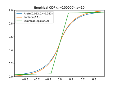
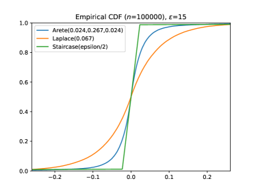
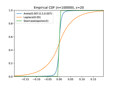
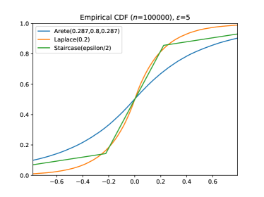
Figure 2: Empirical cumulative distribution functions for Arete distributions parameterized according to Lemma 1.3 for various values of ε𝜀\varepsilon, compared to two known ε𝜀\varepsilon-differentially noise distributions: Laplace(1/ε1𝜀1/\varepsilon), which is infinitely divisible, and a Staircase distribution (not infinitely divisible) parameterized to be (ε+o(1))𝜀𝑜1(\varepsilon+o(1))-differentially private at neighbor distance Δ=1+o(1)Δ1𝑜1\Delta=1+o(1). The values of ε<20𝜀20\varepsilon<20 are for illustration only, since they are too small for Lemma 1.3 to apply.

Let the Arete distribution Arete(α,θ,λ)𝐴𝑟𝑒𝑡𝑒𝛼𝜃𝜆Arete(\alpha,\theta,\lambda) be as in Definition 1.1 (and formally, Definition 3.5) with density function fAsubscript𝑓𝐴f_{A}. In Section 4.3 we show the following result:

Lemma 1.3.

For every choice of Δ2/eΔ2𝑒\Delta\geq 2/e and ε20+4ln(Δ)𝜀204Δ\varepsilon\geq 20+4\ln(\Delta) there exist parameters α,β,λ>0𝛼𝛽𝜆0\alpha,\beta,\lambda>0 such that:

  • For every choice of t,a𝑡𝑎t,a\in\mathbb{R} with |a|Δ𝑎Δ|a|\leq\Delta, eεfA(t)fA(t+a)eεsuperscript𝑒𝜀subscript𝑓𝐴𝑡subscript𝑓𝐴𝑡𝑎superscript𝑒𝜀e^{-\varepsilon}\leq\frac{f_{A}(t)}{f_{A}(t+a)}\leq e^{\varepsilon}:

  • For ZArete(α,θ,λ)similar-to𝑍𝐴𝑟𝑒𝑡𝑒𝛼𝜃𝜆Z\sim Arete(\alpha,\theta,\lambda), E[|Z|]=O(Δeε/4)E𝑍𝑂Δsuperscript𝑒𝜀4\operatorname{\operatorname{E}}[|Z|]=O(\Delta e^{-\varepsilon/4}) and Var[Z]=O(Δ2eε/4)Var𝑍𝑂superscriptΔ2superscript𝑒𝜀4\operatorname{\operatorname{Var}}[Z]=O(\Delta^{2}e^{-\varepsilon/4}).

Parameters α=eε/4,θ=4Δεformulae-sequence𝛼superscript𝑒𝜀4𝜃4Δ𝜀\alpha=e^{-\varepsilon/4},\theta=\frac{4\Delta}{\varepsilon} and λ=eε/4𝜆superscript𝑒𝜀4\lambda=e^{-\varepsilon/4} suffice.

The condition Δ2/eΔ2𝑒\Delta\geq 2/e is not essential in the sense that we may always scale the noise by a factor ΔΔ\Delta, which means that it is enough to consider sensitivity 1. This also means that ε20𝜀20\varepsilon\geq 20 suffices if we use a scaled Arete distribution.

Figure 2 shows empirical cumulative distribution functions for Arete distributions derived from Lemma 1.3. The code for generating these plots, as well as all other plots in this paper, can be found on GitHub.https://github.com/rasmus-pagh/alt22-code

The following corollary, shown in Section 3.2, says that adding noise from the Arete distribution gives an ε𝜀\varepsilon-differentially private mechanism. We refer to Section B.2 for details about differential privacy and the definition of the sensitivity of a query.

Definition 1.4 (The Arete mechanism).

Let x𝒳d𝑥superscript𝒳𝑑x\in\mathcal{X}^{d} be an input and q:𝒳d:𝑞superscript𝒳𝑑q:\mathcal{X}^{d}\rightarrow\mathbb{R} a query with sensitivity bounded by Δ2/eΔ2𝑒\Delta\geq 2/e. Given parameters α,θ,λ𝛼𝜃𝜆\alpha,\theta,\lambda, the Arete mechanism Arete(x)subscript𝐴𝑟𝑒𝑡𝑒𝑥\mathcal{M}_{Arete}(x) samples ZArete(α,θ,λ)similar-to𝑍𝐴𝑟𝑒𝑡𝑒𝛼𝜃𝜆Z\sim Arete(\alpha,\theta,\lambda) and returns q(x)+Z𝑞𝑥𝑍q(x)+Z.

Corollary 1.5.

The Arete mechanism Aretesubscript𝐴𝑟𝑒𝑡𝑒\mathcal{M}_{Arete} with parameters as specified in Lemma 1.3 has expected error O(Δeε/4)𝑂Δsuperscript𝑒𝜀4O(\Delta e^{-\varepsilon/4}) and is ε𝜀\varepsilon-differentially private.

Discussion of Large Values of ε𝜀\varepsilon. Values of ε𝜀\varepsilon larger than one often appear in practice. Examples of deployments using large values of ε𝜀\varepsilon include Google’s RAPPOR with ε𝜀\varepsilon up to 9, Apple’s MacOS with ε=6𝜀6\varepsilon=6, iOS 10 with ε=14𝜀14\varepsilon=14 (Greenberg, 2017), and US Census Bureau with ε𝜀\varepsilon up to 19.619.619.6.https://www.census.gov/newsroom/press-releases/2021/2020-census-key-parameters.html

These examples are not directly comparable to our setting since they deal with either local differential privacy (data of a single user), or with the release of many statistics (rather than a single aggregate). However, we note that mechanisms in the low-privacy regime can often be “boosted”, e.g. using sampling (Balle et al., 2018) or shuffling (Erlingsson et al., 2019), to obtain a mechanism with a better privacy parameter. If sampling is used to improve privacy we will of course get noise due to sampling error, and this will dominate the total error in most cases. One way to use our result (with secure aggregation) is to essentially match the error of estimating a sum from a sample, getting privacy almost for free when the sample is much smaller than the whole data set.

The lower bound on ε𝜀\varepsilon in Lemma 1.3 is high, but we note that empirically we achieve differential privacy for significantly lower values of ε𝜀\varepsilon (see Section 5).

2 Related Works

A fundamental question is what can be said about the tradeoff between error and privacy. Hardt and Talwar (2010) study this tradeoff for linear queries, showing a lower bound of Ω(1/ε)Ω1𝜀\Omega(1/\varepsilon) for worst case expected 2subscript2\ell_{2}-norm of noise (std. deviation) under the constraint of ε𝜀\varepsilon-differential privacy for small ε𝜀\varepsilon. Nikolov et al. (2013) extend the work of (Hardt and Talwar, 2010) to the tradeoff between error and (ε,δ)𝜀𝛿(\varepsilon,\delta)-differential privacy. For error that can be a general function of the added noise, Gupte and Sundararajan (2010) and Ghosh, Roughgarden, and Sundararajan (2012) introduced the Geometric Mechanism for counting queries (integer valued) with sensitivity 1, showing that the optimal noise has a (symmetric) Geometric distribution with error (standard deviation) Θ(eε/2)Θsuperscript𝑒𝜀2\Theta(e^{-\varepsilon/2}). Brenner and Nissim (2010) extend these results, showing that for general queries there is no optimal mechanism for ε𝜀\varepsilon-differential privacy. In the high privacy regime, Geng and Viswanath (2016b) present a (near) optimal mechanism for integer-valued vector queries for (ε,δ)𝜀𝛿(\varepsilon,\delta)-differential privacy, achieving error (for single-dimensional queries) Θ(min{1/ε,1/δ})Θ1𝜀1𝛿\Theta(\min\{1/\varepsilon,1/\delta\}) for small ε𝜀\varepsilon and δ𝛿\delta. Though the geometric mechanism yields optimal error in the discrete setting, and is infinitely divisible (Goryczka and Xiong, 2017), it does not seem to generalize to a differentially private, infinitely divisible noise distribution in the real-valued setting. Recently, Kairouz et al. (2021) studied a distributed, discrete version of the Gaussian mechanism, which has good composition properties. This mechanism is not aimed at the low privacy regime, and does not have error that decreases exponentially as ε𝜀\varepsilon grows.

Generalizing to real-valued 1-dimensional queries with arbitrary sensitivity, Geng and Viswanath (2016a) introduced the ε𝜀\varepsilon-differentially private Staircase mechanism (see Lemma B.7), which adds noise from the Staircase distribution – a geometric mixture of uniform distributions. The density function of the Staircase distribution, fSCsubscript𝑓𝑆𝐶f_{SC}, is a piece-wise continuous step (or “staircase-shaped”) function, symmetric around zero, with geometrically decaying density as a function of the distance from zero. The staircase mechanism circumvents a lower bound of Koufogiannis et al. (2015) on “Lipschitz” differential privacy, which requires the privacy loss to be bounded by ε|q(x)q(y)|/Δ𝜀𝑞𝑥𝑞𝑦Δ\varepsilon|q(x)-q(y)|/\Delta, by only bounding the worst case privacy loss for |q(x)q(y)|/Δ1𝑞𝑥𝑞𝑦Δ1|q(x)-q(y)|/\Delta\leq 1.

Geng and Viswanath (2016a) prove that the optimal ε𝜀\varepsilon-differentially private mechanism for single real-valued queries, measuring error as expected magnitude or variance of noise, is not Laplace but rather Staircase distributed: while the Laplace mechanism is asymptotically optimal as ε0𝜀0\varepsilon\rightarrow 0, the Staircase mechanism performs better in the low privacy regime (i.e., for large ε𝜀\varepsilon), as the expected magnitude of the noise is exponentially decreasing in ε𝜀\varepsilon. Specifically, for sensitivity ΔΔ\Delta and for the parameter setting of γ𝛾\gamma optimizing for expected noise magnitude, the Staircase mechanism achieves error Θ(Δeε/2)ΘΔsuperscript𝑒𝜀2\Theta(\Delta e^{-\varepsilon/2}). For the choice of γ𝛾\gamma optimizing for variance, the Staircase mechanism ensures variance of the noise Θ(Δ2e2ε/3)ΘsuperscriptΔ2superscript𝑒2𝜀3\Theta(\Delta^{2}e^{-2\varepsilon/3}). We note that the γ𝛾\gamma optimizing for noise magnitude is not generally the same a for optimizing for variance. The Laplace distribution has expected noise magnitude Θ(Δ/ε)ΘΔ𝜀\Theta(\Delta/\varepsilon) and variance Θ(Δ2/ε2)ΘsuperscriptΔ2superscript𝜀2\Theta(\Delta^{2}/\varepsilon^{2}). In comparison, the expected noise magnitude and variance of the Arete distribution is also exponentially decreasing in ε𝜀\varepsilon, specifically O(Δeε/4)𝑂Δsuperscript𝑒𝜀4O(\Delta e^{-\varepsilon/4}) and O(Δ2eε/4)𝑂superscriptΔ2superscript𝑒𝜀4O(\Delta^{2}e^{-\varepsilon/4}), respectively, for our choice of parameters. The expected error and variance mentioned here are for a single parameter setting for both Laplace and Arete mechanisms.

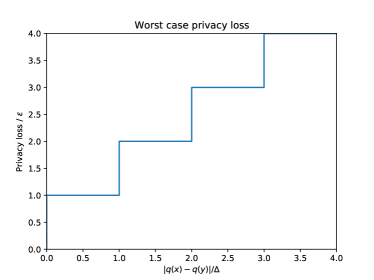
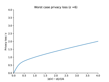
As we want a noise distribution that is implementable in a distributed setting, we limit our interest to noise distributions that are oblivious of the input data and the query output. A nice property of the Arete distribution is that the density function is continuous and so we get a more graceful decrease in privacy than the Staircase mechanism for inputs that are not quite neighboring. We can measure this using the worst case privacy loss, which is the logarithm of the largest ratio between the mechanism’s density functions on inputs x𝑥x and y𝑦y. If |q(x)q(y)|Δ𝑞𝑥𝑞𝑦Δ|q(x)-q(y)|\leq\Delta, inequality (1) implies that the worst case privacy loss is at most ε𝜀\varepsilon. For inputs with |q(x)q(y)|>Δ𝑞𝑥𝑞𝑦Δ|q(x)-q(y)|>\Delta this is no longer guaranteed, but it is still interesting to study how the level of privacy decreases as a function of |q(x)q(y)|𝑞𝑥𝑞𝑦|q(x)-q(y)|. The Staircase mechanism is exactly fitted to the sensitivity of the query such that differential privacy is guaranteed for neighboring inputs, but as soon as |q(x)q(y)|>Δ𝑞𝑥𝑞𝑦Δ|q(x)-q(y)|>\Delta the worst case privacy loss is immediately doubled. The privacy loss increases in a smoother fashion when applying the Arete distribution due to the continuity of the density function (See Figure 3).

\subfigure

[Staircase mechanism] Refer to caption \subfigure[Arete mechanism] Refer to caption

Figure 3: Worst case privacy loss of the Staircase and Arete mechanisms (the latter with ε=6𝜀6\varepsilon=6) as a function of the difference between query outputs. As we have no closed form for the density of the Arete distribution, the plot on the right hand side is a numerical approximation computed by discretizing the involved ΓΓ\Gamma and Laplace distributions and computing the convolution of the discretizations. The privacy loss of the Arete distribution increases rapidly from distance 00 to about Δ/2Δ2\Delta/2 and then increases more slowly from Δ/2Δ2\Delta/2 to ΔΔ\Delta where it reaches ε𝜀\varepsilon. As can be seen the Arete distribution has a smaller privacy loss than the staircase distribution for larger distances |q(x)q(y)|𝑞𝑥𝑞𝑦|q(x)-q(y)|, suggesting that it in fact adds more noise than necessary.

Geng et al. (2015) extend the Staircase mechanism from (Geng and Viswanath, 2016a) to queries in multiple dimensions.

3 The Arete Distribution

This section introduces the Arete distribution and some of its properties. We refer to Appendix B for definitions of probability distributions and differential privacy. The following lemma is well-known from the probability theory literature:

Lemma 3.1.

If X𝑋X and Y𝑌Y are independent, continuous random variables with density functions fXsubscript𝑓𝑋f_{X} and fYsubscript𝑓𝑌f_{Y}, then Z=X+Y𝑍𝑋𝑌Z=X+Y is a continuous random variable where the density is the convolution

fZ(z)=fX(x)fY(zx)𝑑x=fX(zx)fY(x)𝑑x.subscript𝑓𝑍𝑧superscriptsubscriptsubscript𝑓𝑋𝑥subscript𝑓𝑌𝑧𝑥differential-d𝑥=superscriptsubscriptsubscript𝑓𝑋𝑧𝑥subscript𝑓𝑌𝑥differential-d𝑥f_{Z}(z)=\int_{-\infty}^{\infty}f_{X}(x)f_{Y}(z-x)dx\textbf{=}\int_{-\infty}^{\infty}f_{X}(z-x)f_{Y}(x)dx.

The following distribution will be useful in defining the Arete distribution:

Definition 3.2 (The ΓΓΓΓ\Gamma-\Gamma Distribution).

Let X1,X2Γ(α,θ)similar-tosubscript𝑋1subscript𝑋2Γ𝛼𝜃X_{1},X_{2}\sim\Gamma(\alpha,\theta) be independent and consider their difference X:=X1X2assign𝑋subscript𝑋1subscript𝑋2X~{}:=~{}X_{1}~{}-~{}X_{2}. We say that X𝑋X has the ΓΓ(α,θ)ΓΓ𝛼𝜃\Gamma-\Gamma(\alpha,\theta) distribution and the density of X𝑋X is

fΓΓ(α,θ)(t)=0fΓ(α,θ)(t+x)fΓ(α,θ)(x)𝑑x={0fΓ(t+x)fΓ(x)𝑑x,t0|t|fΓ(t+x)fΓ(x)𝑑x,t<0.subscript𝑓ΓΓ𝛼𝜃𝑡superscriptsubscript0subscript𝑓Γ𝛼𝜃𝑡𝑥subscript𝑓Γ𝛼𝜃𝑥differential-d𝑥casessuperscriptsubscript0subscript𝑓Γ𝑡𝑥subscript𝑓Γ𝑥differential-d𝑥𝑡0otherwisesuperscriptsubscript𝑡subscript𝑓Γ𝑡𝑥subscript𝑓Γ𝑥differential-d𝑥𝑡0otherwisef_{\Gamma-\Gamma(\alpha,\theta)}(t)=\int_{0}^{\infty}f_{\Gamma(\alpha,\theta)}(t+x)f_{\Gamma(\alpha,\theta)}(x)dx=\begin{cases}\int_{0}^{\infty}f_{\Gamma}(t+x)f_{\Gamma}(x)dx,\qquad t\geq 0\\ \int_{|t|}^{\infty}f_{\Gamma}(t+x)f_{\Gamma}(x)dx,\qquad t<0.\end{cases}

where the integrals are reduced to the intervals where fΓ(t+x)fΓ(x)subscript𝑓Γ𝑡𝑥subscript𝑓Γ𝑥f_{\Gamma}(t+x)f_{\Gamma}(x) is non-zero.

Lemma 3.3.

The ΓΓΓΓ\Gamma-\Gamma distribution is infinitely divisible: For 2n2𝑛2n independent random variables Xi,YiΓ(α/n,θ)similar-tosubscript𝑋𝑖subscript𝑌𝑖Γ𝛼𝑛𝜃X_{i},Y_{i}\sim\Gamma(\alpha/n,\theta), we have X=i=1n(XiYi)ΓΓ(α,θ)𝑋superscriptsubscript𝑖1𝑛subscript𝑋𝑖subscript𝑌𝑖similar-toΓΓ𝛼𝜃X=\sum_{i=1}^{n}(X_{i}-Y_{i})\sim\Gamma-\Gamma\left(\alpha,\theta\right).

Proof 3.4.

The result follows immediately from infinite divisibility of the ΓΓ\Gamma-distribution.

Definition 3.5 (The Arete distribution).

Let XΓΓ(α,θ)similar-to𝑋ΓΓ𝛼𝜃X\sim\Gamma-\Gamma(\alpha,\theta) and YLaplace(λ)similar-to𝑌𝐿𝑎𝑝𝑙𝑎𝑐𝑒𝜆Y\sim Laplace(\lambda) be independent. Define Z:=X+Yassign𝑍𝑋𝑌Z:=X+Y, then ZArete(α,θ,λ)similar-to𝑍𝐴𝑟𝑒𝑡𝑒𝛼𝜃𝜆Z\sim Arete(\alpha,\theta,\lambda) for α,θ,λ>0𝛼𝜃𝜆0\alpha,\theta,\lambda>0. The density of Z𝑍Z is

fA(α,θ,λ)(t)=fΓΓ(α,θ)(tx)fL(λ)(x)𝑑x=fL(λ)(tx)fΓΓ(α,θ)(x)𝑑x,t.formulae-sequencesubscript𝑓𝐴𝛼𝜃𝜆𝑡superscriptsubscriptsubscript𝑓ΓΓ𝛼𝜃𝑡𝑥subscript𝑓𝐿𝜆𝑥differential-d𝑥superscriptsubscriptsubscript𝑓𝐿𝜆𝑡𝑥subscript𝑓ΓΓ𝛼𝜃𝑥differential-d𝑥𝑡f_{A(\alpha,\theta,\lambda)}(t)=\int_{-\infty}^{\infty}f_{\Gamma-\Gamma(\alpha,\theta)}(t-x)f_{L(\lambda)}(x)dx=\int_{-\infty}^{\infty}f_{L(\lambda)}(t-x)f_{\Gamma-\Gamma(\alpha,\theta)}(x)dx,\quad t\in\mathbb{R}.
Lemma 3.6.

The Arete distribution is infinitely divisible: For 4n4𝑛4n independent random variables X1i,X2iΓ(α/n,θ)similar-tosubscript𝑋1𝑖subscript𝑋2𝑖Γ𝛼𝑛𝜃X_{1i},X_{2i}\sim\Gamma(\alpha/n,\theta) and Y1i,Y2iΓ(1/n,λ)similar-tosubscript𝑌1𝑖subscript𝑌2𝑖Γ1𝑛𝜆Y_{1i},Y_{2i}\sim\Gamma(1/n,\lambda), we have X=i=1n(X1iX2i+(Y1iY2i))Arete(α,θ,λ)𝑋superscriptsubscript𝑖1𝑛subscript𝑋1𝑖subscript𝑋2𝑖subscript𝑌1𝑖subscript𝑌2𝑖similar-to𝐴𝑟𝑒𝑡𝑒𝛼𝜃𝜆X=\sum_{i=1}^{n}(X_{1i}-X_{2i}+(Y_{1i}-Y_{2i}))\sim Arete\left(\alpha,\theta,\lambda\right).

Proof 3.7.

The result follows immediately from infinite divisibility of the Laplace distribution and Lemma 3.3.

Note 3.8.

We remark that we are only interested in 0<α<10𝛼10<\alpha<1. Furthermore, we do not explicitly state the density of the Arete distribution, as there is no simple closed form for the density of the ΓΓΓΓ\Gamma-\Gamma distribution. (It can, however, be expressed in terms of Bessel functions – see (Mathai, 1993).) A similar intuitive way of defining our distribution would be to use a symmetric version of the ΓΓ\Gamma-distribution (two halved ΓΓ\Gamma-distributions put back-to-back at zero), instead of the ΓΓΓΓ\Gamma-\Gamma-distribution. An important property of our distribution is infinite divisibility such that we can draw independent noise shares that sum to a random variable following the Arete distribution. As opposed to our ΓΓΓΓ\Gamma-\Gamma distribution, it is not clear whether a symmetric ΓΓ\Gamma-distribution is infinitely divisible.

3.1 Symmetric Density Functions

We observe some simple properties of the Arete distribution.

Lemma 3.9.

For f,g::𝑓𝑔f,g:\mathbb{R}\rightarrow\mathbb{R}, that are symmetric around 0, i.e., f(x)=f(x)𝑓𝑥𝑓𝑥f(x)=f(-x) and g(x)=g(x)𝑔𝑥𝑔𝑥g(x)~{}=~{}g(-x), we have for any t𝑡t\in\mathbb{R}

f(x)g(tx)𝑑x=f(x)g(|t|x)𝑑x.superscriptsubscript𝑓𝑥𝑔𝑡𝑥differential-d𝑥superscriptsubscript𝑓𝑥𝑔𝑡𝑥differential-d𝑥\int_{-\infty}^{\infty}f(x)g(t-x)dx=\int_{-\infty}^{\infty}f(x)g(|t|-x)dx.

In particular, the convolution fg𝑓𝑔f\ast g is symmetric around 0.

Proof 3.10.

The statement is immediate for t0𝑡0t\geq 0, so suppose t<0𝑡0t<0. Then for any a,b𝑎𝑏a,b\in\mathbb{R}

abf(x)g(tx)𝑑x=abf(x)g(|t|+x)𝑑x=baf(x)g(|t|x)𝑑x=baf(x)g(|t|x)𝑑xsuperscriptsubscript𝑎𝑏𝑓𝑥𝑔𝑡𝑥differential-d𝑥superscriptsubscript𝑎𝑏𝑓𝑥𝑔𝑡𝑥differential-d𝑥superscriptsubscript𝑏𝑎𝑓𝑥𝑔𝑡𝑥differential-d𝑥superscriptsubscript𝑏𝑎𝑓𝑥𝑔𝑡𝑥differential-d𝑥\int_{-a}^{-b}f(x)g(t-x)dx=\int_{-a}^{-b}f(x)g(|t|+x)dx=\int_{b}^{a}f(-x)g(|t|-x)dx=\int_{b}^{a}f(x)g(|t|-x)dx

where first step is by symmetry of g𝑔g, the second step follows from integration by substitution and the last step is by symmetry of f𝑓f. In particular, we may let a𝑎a and b𝑏b be ±plus-or-minus\pm\infty.

Lemma 3.11.

fΓΓsubscript𝑓ΓΓf_{\Gamma-\Gamma} is symmetric around 0.

Proof 3.12.

We prove that fΓΓ(t)=fΓΓ(|t|)subscript𝑓ΓΓ𝑡subscript𝑓ΓΓ𝑡f_{\Gamma-\Gamma}(t)=f_{\Gamma-\Gamma}(|t|) for all t𝑡t\in\mathbb{R}. Clearly, this is the case if t0𝑡0t\geq 0, so suppose t<0𝑡0t<0. By Definition 3.2

fΓΓ(t)=|t|fΓ(t+x)fΓ(x)𝑑x=|t|fΓ(x|t|)fΓ(x)𝑑x=0fΓ(x)fΓ(|t|+x)𝑑x=fΓΓ(|t|).subscript𝑓ΓΓ𝑡superscriptsubscript𝑡subscript𝑓Γ𝑡𝑥subscript𝑓Γ𝑥differential-d𝑥superscriptsubscript𝑡subscript𝑓Γ𝑥𝑡subscript𝑓Γ𝑥differential-d𝑥superscriptsubscript0subscript𝑓Γ𝑥subscript𝑓Γ𝑡𝑥differential-d𝑥subscript𝑓ΓΓ𝑡f_{\Gamma-\Gamma}(t)=\int_{|t|}^{\infty}f_{\Gamma}(t+x)f_{\Gamma}(x)dx=\int_{|t|}^{\infty}f_{\Gamma}(x-|t|)f_{\Gamma}(x)dx=\int_{0}^{\infty}f_{\Gamma}(x)f_{\Gamma}(|t|+x)dx=f_{\Gamma-\Gamma}(|t|).

where the penultimate step follows from integration by substitution with x|t|𝑥𝑡x-|t|.

Corollary 3.13.

fAsubscript𝑓𝐴f_{A} is symmetric around 0.

Proof 3.14.

The result follows directly from symmetry of the density of the Laplace distribution, fLsubscript𝑓𝐿f_{L}, and Lemmas 3.9 and 3.11.

3.2 Properties of the Arete Distribution

We restate the lemma here for convenience: See 1.2

Proof 3.15.

Symmetry of the density function fAsubscript𝑓𝐴f_{A} is proven in Corollary 3.13 and infinite divisibility in Lemma 3.6. Since fΓsubscript𝑓Γf_{\Gamma} and fLsubscript𝑓𝐿f_{L} are continuous, fΓΓsubscript𝑓ΓΓf_{\Gamma-\Gamma} and fAsubscript𝑓𝐴f_{A} are also continuous by Lemma 3.1. We prove that fAsubscript𝑓𝐴f_{A} is monotonely decreasing, i.e., for |t||t|𝑡superscript𝑡|t|\leq|t^{\prime}| we have fA(t)fA(t)subscript𝑓𝐴𝑡subscript𝑓𝐴superscript𝑡f_{A}(t)\geq f_{A}(t^{\prime}). First, we argue that fΓΓsubscript𝑓ΓΓf_{\Gamma-\Gamma} is monotonely decreasing. Recall Definition 3.2 and observe

fΓΓ(t)=0fΓ(|t|+x)fΓ(x)𝑑x,tformulae-sequencesubscript𝑓ΓΓ𝑡superscriptsubscript0subscript𝑓Γ𝑡𝑥subscript𝑓Γ𝑥differential-d𝑥for-all𝑡f_{\Gamma-\Gamma}(t)=\int_{0}^{\infty}f_{\Gamma}(|t|+x)f_{\Gamma}(x)dx,\qquad\forall t\in\mathbb{R}

which is immediate for t0𝑡0t\geq 0 while for t<0𝑡0t<0

fΓΓ(t)=|t|fΓ(|t|+x)fΓ(x)𝑑x=0fΓ(x)fΓ(x+|t|)𝑑xsubscript𝑓ΓΓ𝑡superscriptsubscript𝑡subscript𝑓Γ𝑡𝑥subscript𝑓Γ𝑥differential-d𝑥superscriptsubscript0subscript𝑓Γsuperscript𝑥subscript𝑓Γsuperscript𝑥𝑡differential-dsuperscript𝑥f_{\Gamma-\Gamma}(t)=\int_{|t|}^{\infty}f_{\Gamma}(-|t|+x)f_{\Gamma}(x)dx=\int_{0}^{\infty}f_{\Gamma}(x^{\prime})f_{\Gamma}(x^{\prime}+|t|)dx^{\prime}

where we substituted x:=x|t|assignsuperscript𝑥𝑥𝑡x^{\prime}:=x-|t|. So assume |t||t|𝑡superscript𝑡|t|\leq|t^{\prime}|. Then, since fΓsubscript𝑓Γf_{\Gamma} is monotonely decreasing

fΓΓ(t)=0fΓ(|t|+x)fΓ(x)𝑑x0fΓ(|t|+x)fΓ(x)𝑑x=fΓΓ(t).subscript𝑓ΓΓ𝑡superscriptsubscript0subscript𝑓Γ𝑡𝑥subscript𝑓Γ𝑥differential-d𝑥superscriptsubscript0subscript𝑓Γsuperscript𝑡𝑥subscript𝑓Γ𝑥differential-d𝑥subscript𝑓ΓΓsuperscript𝑡\displaystyle f_{\Gamma-\Gamma}(t)=\int_{0}^{\infty}f_{\Gamma}(|t|+x)f_{\Gamma}(x)dx\geq\int_{0}^{\infty}f_{\Gamma}(|t^{\prime}|+x)f_{\Gamma}(x)dx=f_{\Gamma-\Gamma}(t^{\prime}).

We prove that fAsubscript𝑓𝐴f_{A} is also monotonely decreasing: Assuming that |t||t|𝑡superscript𝑡|t|\leq|t^{\prime}| we prove that fA(t)fA(t)subscript𝑓𝐴𝑡subscript𝑓𝐴superscript𝑡f_{A}(t)~{}\geq~{}f_{A}(t^{\prime}). Recall Definition 3.5 and observe

fA(t)=fΓΓ(|t|x)fL(x)𝑑x=fΓΓ(x)fL(|t|x)𝑑xsubscript𝑓𝐴𝑡superscriptsubscriptsubscript𝑓ΓΓ𝑡𝑥subscript𝑓𝐿𝑥differential-d𝑥superscriptsubscriptsubscript𝑓ΓΓ𝑥subscript𝑓𝐿𝑡𝑥differential-d𝑥f_{A}(t)=\int_{-\infty}^{\infty}f_{\Gamma-\Gamma}(|t|-x)f_{L}(x)dx=\int_{-\infty}^{\infty}f_{\Gamma-\Gamma}(x)f_{L}(|t|-x)dx

which is obvious for t0𝑡0t\geq 0 and since for t<0𝑡0t<0:

fA(t)=fΓΓ(tx)fL(x)𝑑x=fΓΓ(|t|+x)fL(x)𝑑x=fΓΓ(x)fL(|t|x)𝑑xsubscript𝑓𝐴𝑡superscriptsubscriptsubscript𝑓ΓΓ𝑡𝑥subscript𝑓𝐿𝑥differential-d𝑥superscriptsubscriptsubscript𝑓ΓΓ𝑡𝑥subscript𝑓𝐿𝑥differential-d𝑥superscriptsubscriptsubscript𝑓ΓΓsuperscript𝑥subscript𝑓𝐿𝑡superscript𝑥differential-dsuperscript𝑥\displaystyle f_{A}(t)=\int_{-\infty}^{\infty}f_{\Gamma-\Gamma}(t-x)f_{L}(x)dx=\int_{-\infty}^{\infty}f_{\Gamma-\Gamma}(|t|+x)f_{L}(x)dx=\int_{-\infty}^{\infty}f_{\Gamma-\Gamma}(x^{\prime})f_{L}(|t|-x^{\prime})dx^{\prime}

using that fΓΓsubscript𝑓ΓΓf_{\Gamma-\Gamma} and fLsubscript𝑓𝐿f_{L} are symmetric and a substitution with x:=|t|+xassignsuperscript𝑥𝑡𝑥x^{\prime}:=|t|+x. A similar argument can be made if the convolution is flipped. We conclude that

fA(t)=fΓΓ(|t|x)fL(x)𝑑xfΓΓ(|t|x)fL(x)𝑑x=fA(t)subscript𝑓𝐴𝑡superscriptsubscriptsubscript𝑓ΓΓ𝑡𝑥subscript𝑓𝐿𝑥differential-d𝑥superscriptsubscriptsubscript𝑓ΓΓsuperscript𝑡𝑥subscript𝑓𝐿𝑥differential-d𝑥subscript𝑓𝐴superscript𝑡\displaystyle f_{A}(t)=\int_{-\infty}^{\infty}f_{\Gamma-\Gamma}(|t|-x)f_{L}(x)dx\geq\int_{-\infty}^{\infty}f_{\Gamma-\Gamma}(|t^{\prime}|-x)f_{L}(x)dx=f_{A}(t^{\prime})

using that fΓΓsubscript𝑓ΓΓf_{\Gamma-\Gamma} is monotonely decreasing.

We finally assume Lemma 1.3 and prove Corollary 1.5, restated here for convenience. The proof of Lemma 1.3 is given in Section 4. See 1.5

Proof 3.16.

The expected error bound follows directly from the bound on E[|Z|]E𝑍\operatorname{\operatorname{E}}[|Z|] in Lemma 1.3. For the claim of differential privacy, let x,x𝑥superscript𝑥x,x^{\prime}\in\mathbb{R} with |xx|1𝑥superscript𝑥1|x-x^{\prime}|\leq 1. We show that for any subset S𝑆S\subset\mathbb{R}

Pr[Arete(x)S]eεPr[Arete(x)S].Prsubscript𝐴𝑟𝑒𝑡𝑒𝑥𝑆superscript𝑒𝜀Prsubscript𝐴𝑟𝑒𝑡𝑒superscript𝑥𝑆\displaystyle\Pr[\mathcal{M}_{Arete}(x)\in S]\leq e^{\varepsilon}\Pr[\mathcal{M}_{Arete}(x^{\prime})\in S]. (2)

Let noise ZArete(α,θ,λ)similar-to𝑍𝐴𝑟𝑒𝑡𝑒𝛼𝜃𝜆Z\sim Arete(\alpha,\theta,\lambda) for parameters α,θ,λ𝛼𝜃𝜆\alpha,\theta,\lambda as in Lemma 1.3.
Define S:=Sq(x)={sq(x):sS}assignsuperscript𝑆𝑆𝑞𝑥conditional-set𝑠𝑞𝑥𝑠𝑆S^{\prime}~{}:=~{}S-q(x)~{}=~{}\{s~{}-~{}q(x):~{}s\in S\}, then:

Pr[Arete(x)S]Pr[Arete(x)S]=SfA(z)𝑑zSfA(z+q(x)q(x))𝑑zSfA(|z|)𝑑zSfA(|z|+|q(x)q(x)|)𝑑zPrsubscript𝐴𝑟𝑒𝑡𝑒𝑥𝑆Prsubscript𝐴𝑟𝑒𝑡𝑒superscript𝑥𝑆subscriptsuperscript𝑆subscript𝑓𝐴𝑧differential-d𝑧subscriptsuperscript𝑆subscript𝑓𝐴𝑧𝑞superscript𝑥𝑞𝑥differential-d𝑧subscriptsuperscript𝑆subscript𝑓𝐴𝑧differential-d𝑧subscriptsuperscript𝑆subscript𝑓𝐴𝑧𝑞superscript𝑥𝑞𝑥differential-d𝑧\displaystyle\frac{\Pr[\mathcal{M}_{Arete}(x)\in S]}{\Pr[\mathcal{M}_{Arete}(x^{\prime})\in S]}=\frac{\int_{S^{\prime}}f_{A}(z)dz}{\int_{S^{\prime}}f_{A}(z+q(x^{\prime})-q(x))dz}\leq\frac{\int_{S^{\prime}}f_{A}(|z|)dz}{\int_{S^{\prime}}f_{A}(|z|+|q(x^{\prime})-q(x)|)dz}

where we used symmetry of fAsubscript𝑓𝐴f_{A}, the triangle inequality, and the fact that fA(t)subscript𝑓𝐴𝑡f_{A}(t) is decreasing for t>0𝑡0t>0. By assumption |q(x)q(x)|Δ𝑞𝑥𝑞superscript𝑥Δ|q(x)-q(x^{\prime})|\leq\Delta. Lemma 1.3 says that fA(t)/fA(t+a)eεsubscript𝑓𝐴𝑡subscript𝑓𝐴𝑡𝑎superscript𝑒𝜀f_{A}(t)/f_{A}(t+a)\leq e^{\varepsilon} for all t𝑡t\in\mathbb{R} and aΔ𝑎Δa\leq\Delta, and so we get

SfA(|z|)𝑑zSfA(|z|+|q(x)q(x)|)𝑑zSeεfA(|z|+Δ)𝑑zSfA(|z|+|q(x)q(x)|)𝑑zeε.subscriptsuperscript𝑆subscript𝑓𝐴𝑧differential-d𝑧subscriptsuperscript𝑆subscript𝑓𝐴𝑧𝑞superscript𝑥𝑞𝑥differential-d𝑧subscriptsuperscript𝑆superscript𝑒𝜀subscript𝑓𝐴𝑧Δdifferential-d𝑧subscriptsuperscript𝑆subscript𝑓𝐴𝑧𝑞superscript𝑥𝑞𝑥differential-d𝑧superscript𝑒𝜀\displaystyle\frac{\int_{S^{\prime}}f_{A}(|z|)dz}{\int_{S^{\prime}}f_{A}(|z|+|q(x^{\prime})-q(x)|)dz}\leq\frac{\int_{S^{\prime}}e^{\varepsilon}f_{A}(|z|+\Delta)dz}{\int_{S^{\prime}}f_{A}(|z|+|q(x^{\prime})-q(x)|)dz}\leq e^{\varepsilon}.

The first inequality in (2) follows by symmetry.

4 Proof of Main Lemma

In the remaining part of this section we prove a number of theoretical lemmas, that will help prove our main result, Lemma 1.3. The bulk of the analysis is the proof of the first bullet point of Lemma 1.3, showing that the given parameters α,θ,λ>0𝛼𝜃𝜆0\alpha,\theta,\lambda>0 suffice to bound fA(t)/fA(t+a)subscript𝑓𝐴𝑡subscript𝑓𝐴𝑡𝑎f_{A}(t)/f_{A}(t+a) for all t,a𝑡𝑎t,a\in\mathbb{R}, |a|Δ𝑎Δ|a|\leq\Delta. We break this part of the analysis down in this section. The intuition behind the structure is as follows: We first remark that (to the best of our knowledge) there is no simple expression for the density of the ΓΓΓΓ\Gamma-\Gamma distribution (see Note 3.8). Hence, we will show upper and lower bounds for fΓΓsubscript𝑓ΓΓf_{\Gamma-\Gamma} and use these to bound the ratio fA(t)/fA(t+a)subscript𝑓𝐴𝑡subscript𝑓𝐴𝑡𝑎f_{A}(t)/f_{A}(t+a). As discussed earlier, we have not optimized for constants, and as our proof includes several steps of bounding, our analysis may not be tight, thus leading to the high value of ε𝜀\varepsilon required in Lemma 1.3. A tighter analysis is likely to allow for a better setting of parameters α,θ,λ𝛼𝜃𝜆\alpha,\theta,\lambda and a smaller ε𝜀\varepsilon. We give the proof of Lemma 1.3 in Section 4.3.

4.1 Bounds on Density of ΓΓΓΓ\Gamma-\Gamma Distribution

We first derive upper and lower bounds on the density function of the ΓΓΓΓ\Gamma-\Gamma distribution (see Section B for definitions).

Lemma 4.1.

For any t𝑡t\in\mathbb{R} and any ζΓ>0subscript𝜁Γ0\operatorname{\zeta_{\Gamma}}>0

fΓ(|t|+ζΓ)cζΓfΓΓ(t)fΓ(|t|)wherecζΓ:=0ζΓfΓ(x)𝑑x.formulae-sequencesubscript𝑓Γ𝑡subscript𝜁Γsubscript𝑐subscript𝜁Γsubscript𝑓ΓΓ𝑡subscript𝑓Γ𝑡assignwheresubscript𝑐subscript𝜁Γsuperscriptsubscript0subscript𝜁Γsubscript𝑓Γ𝑥differential-d𝑥f_{\Gamma}(|t|+\operatorname{\zeta_{\Gamma}})c_{\operatorname{\zeta_{\Gamma}}}\leq f_{\Gamma-\Gamma}(t)\leq f_{\Gamma}(|t|)\qquad\text{where}\qquad c_{\operatorname{\zeta_{\Gamma}}}:=\int_{0}^{\operatorname{\zeta_{\Gamma}}}f_{\Gamma}(x)dx\enspace.
Proof 4.2.

Recall Definition 3.2 and Lemma 3.11 and let t𝑡t\in\mathbb{R}. For the upper bound, we have

fΓΓ(t)subscript𝑓ΓΓ𝑡\displaystyle f_{\Gamma-\Gamma}(t) =0fΓ(|t|+x)fΓ(x)𝑑x<fΓ(|t|)0fΓ(x)𝑑x=fΓ(|t|).absentsuperscriptsubscript0subscript𝑓Γ𝑡𝑥subscript𝑓Γ𝑥differential-d𝑥subscript𝑓Γ𝑡superscriptsubscript0subscript𝑓Γ𝑥differential-d𝑥subscript𝑓Γ𝑡\displaystyle=\int_{0}^{\infty}f_{\Gamma}(|t|+x)f_{\Gamma}(x)dx<f_{\Gamma}(|t|)\int_{0}^{\infty}f_{\Gamma}(x)dx=f_{\Gamma}(|t|).

For the lower bound we have for any ζΓ>0subscript𝜁Γ0\operatorname{\zeta_{\Gamma}}>0

fΓΓ(t)=0fΓ(|t|+x)fΓ(x)𝑑x0ζΓfΓ(|t|+x)fΓ(x)𝑑xfΓ(|t|+ζΓ)0ζΓfΓ(x)𝑑x.subscript𝑓ΓΓ𝑡superscriptsubscript0subscript𝑓Γ𝑡𝑥subscript𝑓Γ𝑥differential-d𝑥superscriptsubscript0subscript𝜁Γsubscript𝑓Γ𝑡𝑥subscript𝑓Γ𝑥differential-d𝑥subscript𝑓Γ𝑡subscript𝜁Γsuperscriptsubscript0subscript𝜁Γsubscript𝑓Γ𝑥differential-d𝑥\displaystyle f_{\Gamma-\Gamma}(t)=\int_{0}^{\infty}f_{\Gamma}(|t|+x)f_{\Gamma}(x)dx\geq\int_{0}^{\operatorname{\zeta_{\Gamma}}}f_{\Gamma}(|t|+x)f_{\Gamma}(x)dx\geq f_{\Gamma}(|t|+\operatorname{\zeta_{\Gamma}})\int_{0}^{\operatorname{\zeta_{\Gamma}}}f_{\Gamma}(x)dx\enspace.

4.2 Bounds on Density of Arete Distribution

In this section we show that for Δ>0Δ0\Delta>0 and setting of parameters α,θ,λ𝛼𝜃𝜆\alpha,\theta,\lambda and for large enough ε𝜀\varepsilon:

eεfA(t)/fA(t+Δ)eε,t.formulae-sequencesuperscript𝑒𝜀subscript𝑓𝐴𝑡subscript𝑓𝐴𝑡Δsuperscript𝑒𝜀for-all𝑡\displaystyle e^{-\varepsilon}~{}\leq~{}f_{A}(t)/f_{A}(t+\Delta)~{}\leq~{}e^{\varepsilon},\qquad\forall t\in\mathbb{R}. (3)

We remark that by monotonicity of the density of the Arete distribution, if we show (3) it follows that fAsubscript𝑓𝐴f_{A} satisfies (1): Take any a𝑎a\in\mathbb{R} such that |a|Δ𝑎Δ|a|\leq\Delta and suppose without loss of generality that f(t)f(t+a)𝑓𝑡𝑓𝑡𝑎f(t)\geq f(t+a) (if this is not the case, substitute t:=|t|aassignsuperscript𝑡𝑡𝑎t^{\prime}:=|t|-a, such that f(t)f(t+a)𝑓superscript𝑡𝑓superscript𝑡𝑎f(t^{\prime})\geq f(t^{\prime}+a)). Then eεf(t)f(t+a)superscript𝑒𝜀𝑓𝑡𝑓𝑡𝑎e^{-\varepsilon}\leq\frac{f(t)}{f(t+a)}. We prove that f(t+a)f(t+Δ)𝑓𝑡𝑎𝑓𝑡Δf(t+a)\geq f(t+\Delta) ensuring f(t)f(t+a)f(t)f(t+Δ)eε𝑓𝑡𝑓𝑡𝑎𝑓𝑡𝑓𝑡Δsuperscript𝑒𝜀\frac{f(t)}{f(t+a)}\leq\frac{f(t)}{f(t+\Delta)}\leq e^{\varepsilon}, which finishes the argument: by assumption f(t)f(t+a)𝑓𝑡𝑓𝑡𝑎f(t)\geq f(t+a) and so |t||t+a|𝑡𝑡𝑎|t|\leq|t+a|, further implying that ta/2𝑡𝑎2t\geq-a/2. Hence, as |a|Δ𝑎Δ|a|\leq\Delta we have |t+Δ||t+a|𝑡Δ𝑡𝑎|t+\Delta|\geq|t+a| and so we conclude that f(t+a)f(t+Δ)𝑓𝑡𝑎𝑓𝑡Δf(t+a)\geq f(t+\Delta) as wanted.

Throughout the section we assume that |t||t+Δ|𝑡𝑡Δ|t|\leq|t+\Delta| (and so tΔ/2𝑡Δ2t\geq-\Delta/2). For such t𝑡t, fA(t)fA(t+Δ)subscript𝑓𝐴𝑡subscript𝑓𝐴𝑡Δf_{A}(t)~{}\geq~{}f_{A}(t+\Delta) and so the first inequality in (3) is immediate. Hence, we put our focus toward proving the latter inequality. If |t+Δ||t|𝑡Δ𝑡|t+\Delta|\leq|t|, the result follows by symmetry of fAsubscript𝑓𝐴f_{A} (Corollary 3.13).

We start with the following lower bound on the density fAsubscript𝑓𝐴f_{A}:

Lemma 4.3.

Let ζΓsubscript𝜁Γ\operatorname{\zeta_{\Gamma}} and cζΓsubscript𝑐subscript𝜁Γc_{\operatorname{\zeta_{\Gamma}}} be as in Lemma 4.1 and assume λΔ/ln(2)𝜆Δ2\lambda~{}\leq~{}\Delta/\ln(2) for Δ>0Δ0\Delta>0. For Δ/2tΔ2𝑡-\Delta/2~{}\leq~{}t\in\mathbb{R}

fA(t+Δ)fΓ(|t+Δ|+ζΓ)cζΓcLwherecL:=1/4.formulae-sequencesubscript𝑓𝐴𝑡Δsubscript𝑓Γ𝑡Δsubscript𝜁Γsubscript𝑐subscript𝜁Γsubscript𝑐𝐿whereassignsubscript𝑐𝐿14f_{A}(t+\Delta)\geq f_{\Gamma}(|t+\Delta|+\operatorname{\zeta_{\Gamma}})c_{\operatorname{\zeta_{\Gamma}}}c_{L}\qquad\text{where}\qquad c_{L}:=1/4.
Proof 4.4.

By Definition 3.5 and Lemma 4.1 we have

fA(t+Δ)subscript𝑓𝐴𝑡Δ\displaystyle f_{A}(t+\Delta) =fΓΓ(t+Δx)fL(x)𝑑xfΓ(|t+Δx|+ζΓ)cζΓfL(x)𝑑xabsentsuperscriptsubscriptsubscript𝑓ΓΓ𝑡Δ𝑥subscript𝑓𝐿𝑥differential-d𝑥superscriptsubscriptsubscript𝑓Γ𝑡Δ𝑥subscript𝜁Γsubscript𝑐subscript𝜁Γsubscript𝑓𝐿𝑥differential-d𝑥\displaystyle=\int_{-\infty}^{\infty}f_{\Gamma-\Gamma}(t+\Delta-x)f_{L}(x)dx\geq\int_{-\infty}^{\infty}f_{\Gamma}(|t+\Delta-x|+\operatorname{\zeta_{\Gamma}})c_{\operatorname{\zeta_{\Gamma}}}f_{L}(x)dx
cζΓ02(t+Δ)fΓ(|t+Δx|+ζΓ)fL(x)𝑑xcζΓfΓ(t+Δ+ζΓ)02(t+Δ)fL(x)𝑑x,absentsubscript𝑐subscript𝜁Γsuperscriptsubscript02𝑡Δsubscript𝑓Γ𝑡Δ𝑥subscript𝜁Γsubscript𝑓𝐿𝑥differential-d𝑥subscript𝑐subscript𝜁Γsubscript𝑓Γ𝑡Δsubscript𝜁Γsuperscriptsubscript02𝑡Δsubscript𝑓𝐿𝑥differential-d𝑥\displaystyle\geq c_{\operatorname{\zeta_{\Gamma}}}\int_{0}^{2(t+\Delta)}f_{\Gamma}(|t+\Delta-x|+\operatorname{\zeta_{\Gamma}})f_{L}(x)dx\geq c_{\operatorname{\zeta_{\Gamma}}}f_{\Gamma}(t+\Delta+\operatorname{\zeta_{\Gamma}})\int_{0}^{2(t+\Delta)}f_{L}(x)dx,

where we used that fΓ(|t+Δx|+ζΓ)fΓ(|t+Δ|+ζΓ)subscript𝑓Γ𝑡Δ𝑥subscript𝜁Γsubscript𝑓Γ𝑡Δsubscript𝜁Γf_{\Gamma}(|t+\Delta-x|+\operatorname{\zeta_{\Gamma}})\geq f_{\Gamma}(|t+\Delta|+\operatorname{\zeta_{\Gamma}}) for x(0,2(t+Δ))𝑥02𝑡Δx\in(0,2(t+\Delta)) and that by assumption t+ΔΔ/2𝑡ΔΔ2t+\Delta\geq\Delta/2 allowing us to remove the absolute value signs. Again using that t+ΔΔ/2𝑡ΔΔ2t+\Delta\geq\Delta/2

02(t+Δ)fL(x)𝑑x0ΔfL(λ)(x)𝑑x=120ΔfExp(λ)(x)𝑑x14,λ<Δ/ln(2)formulae-sequencesuperscriptsubscript02𝑡Δsubscript𝑓𝐿𝑥differential-d𝑥superscriptsubscript0Δsubscript𝑓𝐿𝜆𝑥differential-d𝑥12superscriptsubscript0Δsubscript𝑓𝐸𝑥𝑝𝜆𝑥differential-d𝑥14𝜆Δ2\int_{0}^{2(t+\Delta)}f_{L}(x)dx\geq\int_{0}^{\Delta}f_{L(\lambda)}(x)dx=\frac{1}{2}\int_{0}^{\Delta}f_{Exp(\lambda)}(x)dx\geq\frac{1}{4},\qquad\lambda<\Delta/\ln(2)

where we noticed that on the positive reals, the density function of the Laplace distribution is 1/2121/2 times the density function of the Exponential distribution, and used that the median of the latter is ln(2)λ2𝜆\ln(2)\lambda, so that the last inequality is true as long as ln(2)λΔ2𝜆Δ\ln(2)\lambda\leq\Delta. Hence,

fA(t+Δ)cζΓfΓ(t+Δ+ζΓ)1/4.subscript𝑓𝐴𝑡Δsubscript𝑐subscript𝜁Γsubscript𝑓Γ𝑡Δsubscript𝜁Γ14f_{A}(t+\Delta)\geq c_{\operatorname{\zeta_{\Gamma}}}f_{\Gamma}(t+\Delta+\operatorname{\zeta_{\Gamma}})1/4.

Defining cL:=1/4assignsubscript𝑐𝐿14c_{L}:=1/4 finishes the proof.

The following three lemmas are technical and give upper bounds for the ratio fA(t)/fA(t+Δ)subscript𝑓𝐴𝑡subscript𝑓𝐴𝑡Δf_{A}(t)~{}/~{}f_{A}(t~{}+~{}\Delta); first for large and small |t|𝑡|t| separately in Lemmas 4.5 and 4.7 (i.e., for t𝑡t close to and far from 0, where ”close to/far from” is quantified by a parameter ζusubscript𝜁u\operatorname{\zeta_{u}}, which we will set in Lemma 4.12). We combine these results to an upper bound for general t𝑡t in Lemma 4.9 (still assuming t𝑡t is s.t. fA(t)fA(t+Δ)subscript𝑓𝐴𝑡subscript𝑓𝐴𝑡Δf_{A}(t)\geq f_{A}(t+\Delta)) and finally choose parameters to ensure an upper bound of eεsuperscript𝑒𝜀e^{\varepsilon} in Lemma 4.12, thus satisfying the second inequality of (3). Throughout the next three lemmas we make use the variables ζΓ,cζΓsubscript𝜁Γsubscript𝑐subscript𝜁Γ\operatorname{\zeta_{\Gamma}},c_{\operatorname{\zeta_{\Gamma}}} (from Lemma 4.1) and cLsubscript𝑐𝐿c_{L} (from Lemma 4.3), all of which will be handled in the proof of Lemma 4.12.

Lemma 4.5.

Let ζu>0subscript𝜁u0\operatorname{\zeta_{u}}>0 be given and assume 0<α10𝛼10<\alpha\leq 1. Let ζΓ,cζΓsubscript𝜁Γsubscript𝑐subscript𝜁Γ\operatorname{\zeta_{\Gamma}},c_{\operatorname{\zeta_{\Gamma}}} be as in Lemma 4.1 and cLsubscript𝑐𝐿c_{L} as in Lemma 4.3. Assume 1/λ1/θ1/(ζu+Δ+ζΓ)1𝜆1𝜃1subscript𝜁uΔsubscript𝜁Γ1/\lambda-1/\theta\geq 1/(\operatorname{\zeta_{u}}+\Delta+\operatorname{\zeta_{\Gamma}}) and λΔ/ln(2)𝜆Δ2\lambda\leq\Delta/\ln(2) for Δ>0Δ0\Delta>0. For Δ/2<tΔ2𝑡-\Delta/2<t\in\mathbb{R} with |t|ζu𝑡subscript𝜁u|t|\geq\operatorname{\zeta_{u}} we have

fA(t)fA(t+Δ)e(ζΓ+Δ)/θcζΓ((1+Δ+ζΓζu)+cζuΓ(α)θα2λcLeζu/θ(ζΓ+Δ+ζu)1α)subscript𝑓𝐴𝑡subscript𝑓𝐴𝑡Δsuperscript𝑒subscript𝜁ΓΔ𝜃subscript𝑐subscript𝜁Γ1Δsubscript𝜁Γsubscript𝜁usubscript𝑐subscript𝜁uΓ𝛼superscript𝜃𝛼2𝜆subscript𝑐𝐿superscript𝑒subscript𝜁u𝜃superscriptsubscript𝜁ΓΔsubscript𝜁u1𝛼\displaystyle\frac{f_{A}(t)}{f_{A}(t+\Delta)}\leq\frac{e^{(\operatorname{\zeta_{\Gamma}}+\Delta)/\theta}}{c_{\operatorname{\zeta_{\Gamma}}}}\left(\left(1+\frac{\Delta+\operatorname{\zeta_{\Gamma}}}{\operatorname{\zeta_{u}}}\right)+\frac{c_{\operatorname{\zeta_{u}}}\Gamma(\alpha)\theta^{\alpha}}{2\lambda c_{L}}e^{\operatorname{\zeta_{u}}/\theta}(\operatorname{\zeta_{\Gamma}}+\Delta+\operatorname{\zeta_{u}})^{1-\alpha}\right)

where cζu:=20ζufΓ(x)𝑑xassignsubscript𝑐subscript𝜁u2superscriptsubscript0subscript𝜁usubscript𝑓Γ𝑥differential-d𝑥c_{\operatorname{\zeta_{u}}}:=2\int_{0}^{\operatorname{\zeta_{u}}}f_{\Gamma}(x)dx.

Proof 4.6.

The proof can be found in Appendix C.1.

Lemma 4.7.

Let ζu>0subscript𝜁u0\operatorname{\zeta_{u}}>0 be given and assume 0<α10𝛼10<\alpha\leq 1. Let ζΓ,cζΓsubscript𝜁Γsubscript𝑐subscript𝜁Γ\operatorname{\zeta_{\Gamma}},c_{\operatorname{\zeta_{\Gamma}}} be as in Lemma 4.1 and cLsubscript𝑐𝐿c_{L} as in Lemma 4.3. Assume 1/λ1/θ1/(Δ+ζΓ)1𝜆1𝜃1Δsubscript𝜁Γ1/\lambda-1/\theta\geq 1/(\Delta+\operatorname{\zeta_{\Gamma}}) and λΔ/ln(2)𝜆Δ2\lambda\leq\Delta/\ln(2) for Δ>0Δ0\Delta>0. For Δ/2<tΔ2𝑡-\Delta/2<t\in\mathbb{R} such that |t|ζu𝑡subscript𝜁u|t|\leq\operatorname{\zeta_{u}} we have

fA(t)fA(t+Δ)e(ζΓ+Δ)/θcLcζΓλ(ζu+ζΓ+Δα+Γ(α)θα(ζΓ+Δ)1α)subscript𝑓𝐴𝑡subscript𝑓𝐴𝑡Δsuperscript𝑒subscript𝜁ΓΔ𝜃subscript𝑐𝐿subscript𝑐subscript𝜁Γ𝜆subscript𝜁usubscript𝜁ΓΔ𝛼Γ𝛼superscript𝜃𝛼superscriptsubscript𝜁ΓΔ1𝛼\displaystyle\frac{f_{A}(t)}{f_{A}(t+\Delta)}\leq\frac{e^{(\operatorname{\zeta_{\Gamma}}+\Delta)/\theta}}{c_{L}c_{\operatorname{\zeta_{\Gamma}}}\lambda}\left(\frac{\operatorname{\zeta_{u}}+\operatorname{\zeta_{\Gamma}}+\Delta}{\alpha}+\Gamma(\alpha)\theta^{\alpha}(\operatorname{\zeta_{\Gamma}}+\Delta)^{1-\alpha}\right)
Proof 4.8.

The proof can be found in Appendix C.2.

The following lemma combines Lemmas 4.5 and 4.7 to give an upper bound for general t>Δ/2𝑡Δ2t~{}>~{}-~{}\Delta/2:

Lemma 4.9.

Let ζΓ,cζΓsubscript𝜁Γsubscript𝑐subscript𝜁Γ\operatorname{\zeta_{\Gamma}},c_{\operatorname{\zeta_{\Gamma}}} be as in Lemma 4.1 and cLsubscript𝑐𝐿c_{L} as in Lemma 4.3. Assume 0<α10𝛼10<\alpha\leq 1, θζΓ+1𝜃subscript𝜁Γ1\theta\leq\operatorname{\zeta_{\Gamma}}+1, λmin{θ/2,Δ/ln(2)}𝜆𝜃2Δ2\lambda\leq\min\{\theta/2,\Delta/\ln(2)\} and Γ(α)1/αΓ𝛼1𝛼\Gamma(\alpha)\leq 1/\alpha for Δ>0Δ0\Delta>0. For Δ/2<tΔ2𝑡-\Delta/2<t\in\mathbb{R}

fA(t)fA(t+Δ)subscript𝑓𝐴𝑡subscript𝑓𝐴𝑡Δ\displaystyle\frac{f_{A}(t)}{f_{A}(t+\Delta)} 2e(ζΓ+Δ)/θeα(αθ+ζΓ+Δ)αcζΓcLλabsent2superscript𝑒subscript𝜁ΓΔ𝜃superscript𝑒𝛼𝛼𝜃subscript𝜁ΓΔ𝛼subscript𝑐subscript𝜁Γsubscript𝑐𝐿𝜆\displaystyle\leq\frac{2e^{(\operatorname{\zeta_{\Gamma}}+\Delta)/\theta}e^{\alpha}(\alpha\theta+\operatorname{\zeta_{\Gamma}}+\Delta)}{\alpha c_{\operatorname{\zeta_{\Gamma}}}c_{L}\lambda}
Proof 4.10.

The proof can be found in Appendix C.3.

Note 4.11.

The fact that Γ(α)1/αΓ𝛼1𝛼\Gamma(\alpha)\leq 1/\alpha for 0<α10𝛼10<\alpha\leq 1 follows from Euler’s definition of the Gamma function,

Γ(α)=1αn=1(1+1n)α1+αn,Γ𝛼1𝛼superscriptsubscriptproduct𝑛1superscript11𝑛𝛼1𝛼𝑛\Gamma(\alpha)=\frac{1}{\alpha}\prod_{n=1}^{\infty}\frac{(1+\frac{1}{n})^{\alpha}}{1+\frac{\alpha}{n}},

since (1+1n)α1+αnsuperscript11𝑛𝛼1𝛼𝑛(1+\frac{1}{n})^{\alpha}\leq 1+\frac{\alpha}{n} for any n>0𝑛0n>0 and 0<α10𝛼10<\alpha\leq 1.

We finally choose parameters α,θ,λ𝛼𝜃𝜆\alpha,\theta,\lambda ensuring that the ratio eεf(t)/f(t+Δ)eεsuperscript𝑒𝜀𝑓𝑡𝑓𝑡Δsuperscript𝑒𝜀e^{-\varepsilon}\leq f(t)/f(t+\Delta)\leq e^{\varepsilon} for ε𝜀\varepsilon large enough:

Lemma 4.12.

Suppose ε20+4ln(Δ)𝜀204Δ\varepsilon\geq 20+4\ln(\Delta) for Δ2/eΔ2𝑒\Delta\geq 2/e. Let α=eε/4,θ=4Δεformulae-sequence𝛼superscript𝑒𝜀4𝜃4Δ𝜀\alpha=e^{-\varepsilon/4},\theta=\frac{4\Delta}{\varepsilon} and λ=eε/4𝜆superscript𝑒𝜀4\lambda=e^{-\varepsilon/4}. Then for t𝑡t\in\mathbb{R}

eεfA(t)fA(t+Δ)eε.superscript𝑒𝜀subscript𝑓𝐴𝑡subscript𝑓𝐴𝑡Δsuperscript𝑒𝜀e^{-\varepsilon}\leq\frac{f_{A}(t)}{f_{A}(t+\Delta)}\leq e^{\varepsilon}.
Proof 4.13.

The proof can be found in Appendix C.4.

4.3 Putting Things Together

We restate the lemma here for convenience: See 1.3

Proof 4.14.

The first bullet with the choice of parameters α=eε/4,θ=4Δ/εformulae-sequence𝛼superscript𝑒𝜀4𝜃4Δ𝜀\alpha=e^{-\varepsilon/4},\theta=4\Delta/\varepsilon and λ=eε/4𝜆superscript𝑒𝜀4\lambda=e^{-\varepsilon/4} follow from Lemma 4.12 and monotonicity of fAsubscript𝑓𝐴f_{A} (Lemma 1.2), as described at the beginning of Section 4.2. The second bullet also follows from Lemma 4.12, as the expected error of a random variable Z=X+Y𝑍𝑋𝑌Z~{}=~{}X~{}+~{}Y, where XΓΓ(α,θ)similar-to𝑋ΓΓ𝛼𝜃X\sim\Gamma-\Gamma(\alpha,\theta) and YLaplace(λ)similar-to𝑌𝐿𝑎𝑝𝑙𝑎𝑐𝑒𝜆Y\sim Laplace(\lambda), i.e., ZArete(α,θ,λ)similar-to𝑍𝐴𝑟𝑒𝑡𝑒𝛼𝜃𝜆Z\sim Arete(\alpha,\theta,\lambda), is

E[|Z|]=E[|X1X2+Y|]2E[X1]+E[|Y|]=2αθ+λ=8Δeε/4ε+eε/4=O(Δεeε/4)E𝑍Esubscript𝑋1subscript𝑋2𝑌2Esubscript𝑋1E𝑌2𝛼𝜃𝜆8Δsuperscript𝑒𝜀4𝜀superscript𝑒𝜀4𝑂Δ𝜀superscript𝑒𝜀4\operatorname{\operatorname{E}}[|Z|]=\operatorname{\operatorname{E}}[|X_{1}-X_{2}+Y|]\leq 2\operatorname{\operatorname{E}}[X_{1}]+\operatorname{\operatorname{E}}[|Y|]=2\alpha\theta+\lambda=\frac{8\Delta e^{-\varepsilon/4}}{\varepsilon}+e^{-\varepsilon/4}=O\left(\frac{\Delta}{\varepsilon}e^{-\varepsilon/4}\right)

where X1,X2Γ(α,θ)similar-tosubscript𝑋1subscript𝑋2Γ𝛼𝜃X_{1},X_{2}\sim\Gamma(\alpha,\theta), and similarly, by independence

Var[Z]Var𝑍\displaystyle\operatorname{\operatorname{Var}}[Z] =Var[X+Y]=Var[X1X2+Y]=2Var[X1]+Var[Y]=2αθ2+2λ2absentVar𝑋𝑌Varsubscript𝑋1subscript𝑋2𝑌2Varsubscript𝑋1Var𝑌2𝛼superscript𝜃22superscript𝜆2\displaystyle=\operatorname{\operatorname{Var}}[X+Y]=\operatorname{\operatorname{Var}}[X_{1}-X_{2}+Y]=2\operatorname{\operatorname{Var}}[X_{1}]+\operatorname{\operatorname{Var}}[Y]=2\alpha\theta^{2}+2\lambda^{2}
=216Δ2eε/4ε2+2eε/2=O(Δ2ε2eε/4)absent216superscriptΔ2superscript𝑒𝜀4superscript𝜀22superscript𝑒𝜀2𝑂superscriptΔ2superscript𝜀2superscript𝑒𝜀4\displaystyle=2\frac{16\Delta^{2}e^{-\varepsilon/4}}{\varepsilon^{2}}+2e^{-\varepsilon/2}=O\left(\frac{\Delta^{2}}{\varepsilon^{2}}e^{-\varepsilon/4}\right)

with our choice of parameters. Finally, for ε1/2𝜀12\varepsilon\geq 1/\sqrt{2} (which is significantly smaller than the values of ε𝜀\varepsilon that we are interested in), we may simplify to

E[|Z|]=O(Δeε/4),Var[Z]=O(Δ2eε/4)formulae-sequenceE𝑍𝑂Δsuperscript𝑒𝜀4Var𝑍𝑂superscriptΔ2superscript𝑒𝜀4\operatorname{\operatorname{E}}[|Z|]=O\left(\Delta e^{-\varepsilon/4}\right),\qquad\operatorname{\operatorname{Var}}[Z]=O\left(\Delta^{2}e^{-\varepsilon/4}\right)

thus finishing the proof.

\subfigure

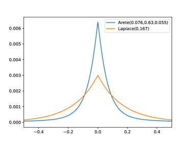
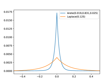
[Densities for ε=6𝜀6\varepsilon=6] Refer to caption \subfigure[Densities for ε=8𝜀8\varepsilon=8] Refer to caption

Figure 4: Density functions for Arete distributions that empirically yield ε𝜀\varepsilon-DP with ε=6𝜀6\varepsilon=6 and ε=8𝜀8\varepsilon=8, respectively. The density functions were approximated by rounding the constituent ΓΓ\Gamma and Laplace distribution values to a multiple of 0.0010.0010.001 and computing the discrete convolution. Parameters were found using a local search heuristic. For comparison, Laplace distributions with the same privacy guarantee have been included and are clearly less concentrated around zero.

5 Conclusion

In this work we have seen a new noise distribution, the Arete distribution, which has a continuous density function, is symmetric around zero, monotonely decreasing for t>0𝑡0t>0, infinitely divisible and has expected absolute value and variance exponentially decreasing in ε𝜀\varepsilon. The Arete distribution yields an ε𝜀\varepsilon-differentially private mechanism, the Arete mechanism, which is an infinitely divisible alternative to the Staircase mechanism (Geng and Viswanath, 2016a) with a continuous density function. The Arete mechanism achieves error comparable to the Staircase mechanism and outperforms the Laplace mechanism (Dwork et al., 2006b) in terms of absolute error and variance in the low privacy regime (for large ε𝜀\varepsilon).

Simulations suggest that the constant factors of the Arete mechanism, with parameters chosen as we have described, can be improved (see Figure 4). We leave open the question of finding an optimal (up to lower order terms), infinitely divisible error distribution for differential privacy in the low privacy regime.

\acks

We thank Thomas Steinke for useful feedback on a previous version of this paper, and the anonymous reviewers for their constructive suggestions. This work was done while both authors were affiliated with BARC, supported by the VILLUM Foundation grant 16582.

References

  • (1) Apple. Apple differential privacy technical overview. https://www.apple.com/privacy/docs/Differential_Privacy_Overview.pdf. Accessed: 2021-07-06.
  • Balle et al. (2018) Borja Balle, Gilles Barthe, and Marco Gaboardi. Privacy amplification by subsampling: Tight analyses via couplings and divergences. In Samy Bengio, Hanna M. Wallach, Hugo Larochelle, Kristen Grauman, Nicolò Cesa-Bianchi, and Roman Garnett, editors, Advances in Neural Information Processing Systems 31: Annual Conference on Neural Information Processing Systems 2018, NeurIPS 2018, December 3-8, 2018, Montréal, Canada, pages 6280–6290, 2018. URL https://proceedings.neurips.cc/paper/2018/hash/3b5020bb891119b9f5130f1fea9bd773-Abstract.html.
  • Balle et al. (2019) Borja Balle, James Bell, Adrià Gascón, and Kobbi Nissim. The privacy blanket of the shuffle model. In Advances in Cryptology - CRYPTO, volume 11693 of Lecture Notes in Computer Science, pages 638–667, 2019. 10.1007/978-3-030-26951-7_22. URL https://doi.org/10.1007/978-3-030-26951-7_22.
  • Balle et al. (2020) Borja Balle, James Bell, Adrià Gascón, and Kobbi Nissim. Private summation in the multi-message shuffle model. In Conference on Computer and Communications Security, CCS, CCS ’20, page 657–676, New York, NY, USA, 2020. ISBN 9781450370899. 10.1145/3372297.3417242. URL https://doi.org/10.1145/3372297.3417242.
  • Bittau et al. (2017) Andrea Bittau, Úlfar Erlingsson, Petros Maniatis, Ilya Mironov, Ananth Raghunathan, David Lie, Mitch Rudominer, Ushasree Kode, Julien Tinnés, and Bernhard Seefeld. Prochlo: Strong privacy for analytics in the crowd. In Symposium on Operating Systems Principles, SOSP, pages 441–459, 2017. 10.1145/3132747.3132769. URL https://doi.org/10.1145/3132747.3132769.
  • Bonawitz et al. (2017) Keith Bonawitz, Vladimir Ivanov, Ben Kreuter, Antonio Marcedone, H. Brendan McMahan, Sarvar Patel, Daniel Ramage, Aaron Segal, and Karn Seth. Practical secure aggregation for privacy-preserving machine learning. In Conference on Computer and Communications Security, CCS, pages 1175–1191, 2017. 10.1145/3133956.3133982. URL https://doi.org/10.1145/3133956.3133982.
  • Brenner and Nissim (2010) Hai Brenner and Kobbi Nissim. Impossibility of differentially private universally optimal mechanisms. In Symposium on Foundations of Computer Science, FOCS, pages 71–80, 2010. 10.1109/FOCS.2010.13. URL https://doi.org/10.1109/FOCS.2010.13.
  • Chan et al. (2012) T.-H. Hubert Chan, Elaine Shi, and Dawn Song. Privacy-preserving stream aggregation with fault tolerance. In Financial Cryptography and Data Security - FC, volume 7397 of Lecture Notes in Computer Science, pages 200–214, 2012. 10.1007/978-3-642-32946-3_15. URL https://doi.org/10.1007/978-3-642-32946-3_15.
  • Chen and Rubin (1986) Jeesen Chen and Herman Rubin. Bounds for the difference between median and mean of Gamma and Poisson distributions. Statistics & Probability Letters, 4(6):281–283, October 1986. URL https://ideas.repec.org/a/eee/stapro/v4y1986i6p281-283.html.
  • Cheu et al. (2019) Albert Cheu, Adam D. Smith, Jonathan R. Ullman, David Zeber, and Maxim Zhilyaev. Distributed differential privacy via shuffling. In Advances in Cryptology, EUROCRYPT, volume 11476 of Lecture Notes in Computer Science, pages 375–403, 2019. 10.1007/978-3-030-17653-2_13. URL https://doi.org/10.1007/978-3-030-17653-2_13.
  • Ding et al. (2017) Bolin Ding, Janardhan Kulkarni, and Sergey Yekhanin. Collecting telemetry data privately. In Advances in Neural Information Processing Systems, NIPS, pages 3571–3580, 2017. URL https://proceedings.neurips.cc/paper/2017/hash/253614bbac999b38b5b60cae531c4969-Abstract.html.
  • Duchi et al. (2013) John C. Duchi, Michael I. Jordan, and Martin J. Wainwright. Local privacy and statistical minimax rates. In 54th Symposium on Foundations of Computer Science, FOCS, pages 429–438, 2013. 10.1109/FOCS.2013.53. URL https://doi.org/10.1109/FOCS.2013.53.
  • Dwork (2008) Cynthia Dwork. Differential privacy: A survey of results. In Manindra Agrawal, Ding-Zhu Du, Zhenhua Duan, and Angsheng Li, editors, Theory and Applications of Models of Computation, TAMC, volume 4978 of Lecture Notes in Computer Science, pages 1–19, 2008. 10.1007/978-3-540-79228-4_1. URL https://doi.org/10.1007/978-3-540-79228-4_1.
  • Dwork and Roth (2014) Cynthia Dwork and Aaron Roth. The algorithmic foundations of differential privacy. Found. Trends Theor. Comput. Sci., 9(3-4):211–407, 2014. 10.1561/0400000042. URL https://doi.org/10.1561/0400000042.
  • Dwork et al. (2006a) Cynthia Dwork, Krishnaram Kenthapadi, Frank McSherry, Ilya Mironov, and Moni Naor. Our data, ourselves: Privacy via distributed noise generation. In Advances in Cryptology, EUROCRYPT, volume 4004 of Lecture Notes in Computer Science, pages 486–503, 2006a. 10.1007/11761679_29. URL https://doi.org/10.1007/11761679_29.
  • Dwork et al. (2006b) Cynthia Dwork, Frank McSherry, Kobbi Nissim, and Adam D. Smith. Calibrating noise to sensitivity in private data analysis. In Theory of Cryptography, TCC, volume 3876 of Lecture Notes in Computer Science, pages 265–284, 2006b. 10.1007/11681878_14. URL https://doi.org/10.1007/11681878_14.
  • Erlingsson et al. (2014) Úlfar Erlingsson, Vasyl Pihur, and Aleksandra Korolova. RAPPOR: randomized aggregatable privacy-preserving ordinal response. In Conference on Computer and Communications Security, pages 1054–1067, 2014. 10.1145/2660267.2660348. URL https://doi.org/10.1145/2660267.2660348.
  • Erlingsson et al. (2019) Úlfar Erlingsson, Vitaly Feldman, Ilya Mironov, Ananth Raghunathan, Kunal Talwar, and Abhradeep Thakurta. Amplification by shuffling: From local to central differential privacy via anonymity. In Symposium on Discrete Algorithms, SODA, pages 2468–2479. SIAM, 2019. 10.1137/1.9781611975482.151. URL https://doi.org/10.1137/1.9781611975482.151.
  • Geng and Viswanath (2016a) Quan Geng and Pramod Viswanath. The optimal noise-adding mechanism in differential privacy. IEEE Trans. Inf. Theory, 62(2):925–951, 2016a. 10.1109/TIT.2015.2504967. URL https://doi.org/10.1109/TIT.2015.2504967.
  • Geng and Viswanath (2016b) Quan Geng and Pramod Viswanath. Optimal noise adding mechanisms for approximate differential privacy. IEEE Trans. Inf. Theory, 62(2):952–969, 2016b. 10.1109/TIT.2015.2504972. URL https://doi.org/10.1109/TIT.2015.2504972.
  • Geng et al. (2015) Quan Geng, Peter Kairouz, Sewoong Oh, and Pramod Viswanath. The staircase mechanism in differential privacy. IEEE J. Sel. Top. Signal Process., 9(7):1176–1184, 2015. 10.1109/JSTSP.2015.2425831. URL https://doi.org/10.1109/JSTSP.2015.2425831.
  • Ghazi et al. (2020a) Badih Ghazi, Noah Golowich, Ravi Kumar, Pasin Manurangsi, Rasmus Pagh, and Ameya Velingker. Pure differentially private summation from anonymous messages. In Information-Theoretic Cryptography, ITC, volume 163 of LIPIcs, pages 15:1–15:23, 2020a. 10.4230/LIPIcs.ITC.2020.15. URL https://doi.org/10.4230/LIPIcs.ITC.2020.15.
  • Ghazi et al. (2020b) Badih Ghazi, Pasin Manurangsi, Rasmus Pagh, and Ameya Velingker. Private aggregation from fewer anonymous messages. In Advances in Cryptology - EUROCRYPT, volume 12106 of Lecture Notes in Computer Science, pages 798–827, 2020b. 10.1007/978-3-030-45724-2_27. URL https://doi.org/10.1007/978-3-030-45724-2_27.
  • Ghazi et al. (2021) Badih Ghazi, Ravi Kumar, Pasin Manurangsi, Rasmus Pagh, and Amer Sinha. Differentially private aggregation in the shuffle model: Almost central accuracy in almost a single message. In International Conference on Machine Learning, ICML, 2021.
  • Ghosh et al. (2012) Arpita Ghosh, Tim Roughgarden, and Mukund Sundararajan. Universally utility-maximizing privacy mechanisms. SIAM J. Comput., 41(6):1673–1693, 2012. 10.1137/09076828X. URL https://doi.org/10.1137/09076828X.
  • Goryczka and Xiong (2017) Slawomir Goryczka and Li Xiong. A comprehensive comparison of multiparty secure additions with differential privacy. Trans. Dependable Secur. Comput., 14(5):463–477, 2017. 10.1109/TDSC.2015.2484326. URL https://doi.org/10.1109/TDSC.2015.2484326.
  • Greenberg (2017) Andy Greenberg. How one of apple’s key privacy safeguards falls short. Wired, 9 2017.
  • Gupte and Sundararajan (2010) Mangesh Gupte and Mukund Sundararajan. Universally optimal privacy mechanisms for minimax agents. In Jan Paredaens and Dirk Van Gucht, editors, Symposium on Principles of Database Systems, PODS, pages 135–146, 2010. 10.1145/1807085.1807105. URL https://doi.org/10.1145/1807085.1807105.
  • Hardt and Talwar (2010) Moritz Hardt and Kunal Talwar. On the geometry of differential privacy. In Symposium on Theory of Computing, STOC, pages 705–714. ACM, 2010. 10.1145/1806689.1806786. URL https://doi.org/10.1145/1806689.1806786.
  • Kairouz et al. (2021) Peter Kairouz, Ziyu Liu, and Thomas Steinke. The distributed discrete gaussian mechanism for federated learning with secure aggregation. In Marina Meila and Tong Zhang, editors, Proceedings of the 38th International Conference on Machine Learning, ICML 2021, 18-24 July 2021, Virtual Event, volume 139 of Proceedings of Machine Learning Research, pages 5201–5212. PMLR, 2021. URL http://proceedings.mlr.press/v139/kairouz21a.html.
  • Kasiviswanathan et al. (2011) Shiva Prasad Kasiviswanathan, Homin K. Lee, Kobbi Nissim, Sofya Raskhodnikova, and Adam D. Smith. What can we learn privately? SIAM J. Comput., 40(3):793–826, 2011. 10.1137/090756090. URL https://doi.org/10.1137/090756090.
  • Koufogiannis et al. (2015) Fragkiskos Koufogiannis, Shuo Han, and George J. Pappas. Optimality of the laplace mechanism in differential privacy. CoRR, abs/1504.00065, 2015. URL http://arxiv.org/abs/1504.00065.
  • Mathai (1993) AM Mathai. On noncentral generalized laplacianness of quadratic forms in normal variables. Journal of multivariate analysis, 45(2):239–246, 1993.
  • McMahan et al. (2017) Brendan McMahan, Eider Moore, Daniel Ramage, Seth Hampson, and Blaise Agüera y Arcas. Communication-efficient learning of deep networks from decentralized data. In Aarti Singh and Xiaojin (Jerry) Zhu, editors, Proceedings of the 20th International Conference on Artificial Intelligence and Statistics (AISTATS), volume 54 of Proceedings of Machine Learning Research, pages 1273–1282. PMLR, 2017. URL http://proceedings.mlr.press/v54/mcmahan17a.html.
  • Nikolov et al. (2013) Aleksandar Nikolov, Kunal Talwar, and Li Zhang. The geometry of differential privacy: the sparse and approximate cases. In Symposium on Theory of Computing Conference, STOC, 2013. 10.1145/2488608.2488652. URL https://doi.org/10.1145/2488608.2488652.
  • Shi et al. (2011) Elaine Shi, T.-H. Hubert Chan, Eleanor Gilbert Rieffel, Richard Chow, and Dawn Song. Privacy-preserving aggregation of time-series data. In Distributed System Security Symposium, NDSS, 2011. URL https://www.ndss-symposium.org/ndss2011/privacy-preserving-aggregation-of-time-series-data.
  • Vadhan (2017) Salil P. Vadhan. The complexity of differential privacy. In Tutorials on the Foundations of Cryptography, pages 347–450. Springer International Publishing, 2017. 10.1007/978-3-319-57048-8_7. URL https://doi.org/10.1007/978-3-319-57048-8_7.
  • Wagh et al. (2021) Sameer Wagh, Xi He, Ashwin Machanavajjhala, and Prateek Mittal. DP-cryptography: marrying differential privacy and cryptography in emerging applications. Commun. ACM, 64(2):84–93, 2021. 10.1145/3418290. URL https://doi.org/10.1145/3418290.
  • Warner (1965) Stanley L Warner. Randomized response: A survey technique for eliminating evasive answer bias. Journal of the American Statistical Association, 60(309):63–69, 1965.
  • (40) Wikipedia. Arete. https://en.wikipedia.org/wiki/Arete.
  • Yao (1982) Andrew Chi-Chih Yao. Protocols for secure computations (extended abstract). In Symposium on Foundations of Computer Science, FOCS, pages 160–164, 1982. 10.1109/SFCS.1982.38. URL https://doi.org/10.1109/SFCS.1982.38.

Appendix A Applications

In differential privacy, two models are prevalent: the central model and the local model. In the central model of differential privacy (Dwork et al., 2006a) all data is held by a single trusted unit who makes the result of a query differentially private before releasing it. This is often done by adding noise to the query result. The central model usually has a very high level of accuracy, but requires a high level of trust. Often, data is split among many players, we refer to these as data owners, and a trusted central unit is not available. This setting is commonly known as the local model of differential privacy (Kasiviswanathan et al., 2011; Warner, 1965; Duchi et al., 2013). In this model, each data owner must ensure privacy for their own data, and so applies a differentially private mechanism locally, which is then forwarded to an analyst who combines all reports to compute an approximate answer to the query. For many queries, the overall error in the local model grows rather quickly as a function of the number of players, significantly limiting utility. For example, while we can achieve constant error in the central model (Dwork et al., 2006b), a count query requires O(n)𝑂𝑛O(\sqrt{n}) error for the same level of privacy as in the central model, where n𝑛n is the number of players (Cheu et al., 2019). The local model is often attractive for data collection as the collecting organizations are not liable for storing sensitive user data in this model – a few examples of deployment include Google’s RAPPOR (Erlingsson et al., 2014), Apple (several features such as Lookup Hints, Emoji suggestion etc.) (Apple, ) and Microsoft Telemetry (Ding et al., 2017).

In order to bridge this trust/utility gap, we may imitate the trusted unit from the centralized setting with cryptographic primitives (Wagh et al., 2021), allowing for differentially private implementations with better utility than in the local model while having lower trust assumptions than in the centralized model. Cryptographic primitives ensure that all parties learn only the output of the computation, while differential privacy further bounds the information leakage from this output, and so the combination gives very strong guarantees. We limit our discussion to the problem of computing the sum of real inputs, which is a basic building block in many other applications. If we can divide the noise among all players we can obtain the same accuracy in a distributed setting as in the central model without the assumption of a trusted aggregator. Luckily, we can divide the noise between the players if the noise distribution 𝒟𝒟\mathcal{D} is infinitely divisible, and so the Arete distribution can be applied in this model.

We discuss differential privacy implementations with two cryptographic primitives: Secure Multiparty Aggregation and Anonymous Communication but note that such implementations come with assumptions about the computational power of the analyst, which are accepted by the security community, but limit the privacy guarantee to computational differential privacy (Wagh et al., 2021).

Secure Multiparty Aggregation

The cryptographic primitive secure multiparty Aggregation, rooted in the work of Yao (Yao, 1982), has often been combined with differential privacy to solve the problem of private real summation, see for example (Shi et al., 2011; Bonawitz et al., 2017; Chan et al., 2012). Goryczka and Xiong (2017) give a comparative study of several protocols for private summation in a distributed setting. These protocols combine common approaches for achieving security (secret sharing, homomorphic encryption and perturbation-based) while each party adds noise shares whose sum follows the Laplace distribution before sharing their data, in order to ensure differential privacy. Continuing their line of work, we may exchange the Laplace noise in (Goryczka and Xiong, 2017) with Arete distributed noise to achieve ε𝜀\varepsilon-differentially private protocols with error exponentially small in ε𝜀\varepsilon.

Anonymous Communication

Another line of work that has received a lot of attention over the past few years is the shuffle model of differential privacy (Bittau et al., 2017; Cheu et al., 2019; Erlingsson et al., 2019). Along with Google’s Prochlo framework, Bittau et al. (2017) introduced the ESA (Encode Shuffle Analyze) framework where each data owner encodes their data before releasing it to a shuffler. The shuffler randomly permutes the encoded inputs and releases the (private) permuted set of data to an (untrusted) analyst, who then performs statistical analysis on the encoded, shuffled data. For recent work on the problem of summation in the shuffle model and a discussion of error/privacy-tradeoff, we refer to for example (Balle et al., 2019, 2020; Ghazi et al., 2020a, 2021, b). Ghazi et al. (2021) propose an (ε,δ)𝜀𝛿(\varepsilon,\delta)-differentially private protocol for summation in the shuffle model for summing reals or integers where each user sends expected 1+o(1)1𝑜11+o(1) messages. The protocol adds discrete Laplace noise (also sometimes called Geometrically distributed noise) and achieves error arbitrarily close to that of the Laplace mechanism (applied in the central model), but do not address the problem of achieving error exponentially decreasing in ε𝜀\varepsilon in the shuffle model. The Arete distribution solves this open problem: as it is infinitely divisible, simply exchange the discrete Laplace noise (the “central” noise distribution in the protocol) with the Arete distribution. This yields:

Corollary A.1 (Differentially private aggregation in the shuffle model.).

Let n𝑛n be a positive integer, and let ε𝜀\varepsilon, δ𝛿\delta be positive real numbers with ε=O(lnn)𝜀𝑂𝑛\varepsilon=O(\ln n). There is an (ε,δ)𝜀𝛿(\varepsilon,\delta)-differentially private aggregation protocol in the shuffle model for inputs in [0,1]01[0,1] having absolute error 1eΩ(ε)11superscript𝑒Ω𝜀1\frac{1}{e^{\Omega(\varepsilon)}-1} in expectation, using O(1+log(1/δ)logn)𝑂11𝛿𝑛O\left(1+\frac{\log(1/\delta)}{\log n}\right) messages per party, each consisting of O(logn)𝑂𝑛O(\log n) bits.

Note. By the post-processing property of differential privacy, we still achieve differential privacy if more than n𝑛n players participate, and so we only need to choose the noise shares based on a lower bound on the number of players in order to ensure differential privacy. Hence, it is not strictly necessary to know the exact number of players in advance.

Appendix B Basic definitions

B.1 Probability Distributions

In this section we state the definitions and basic facts that we need to analyze the Arete distribution. References to further information can be found in (Goryczka and Xiong, 2017).

Definition B.1 (Infinite Divisibility).

A distribution 𝒟𝒟\mathcal{D} is infinitely divisible if, for any random variable X𝑋X with distribution 𝒟𝒟\mathcal{D}, then for every positive integer n𝑛n there exist n𝑛n i.i.d. random variables X1,,Xnsubscript𝑋1subscript𝑋𝑛X_{1},...,X_{n} such that i=1nXisuperscriptsubscript𝑖1𝑛subscript𝑋𝑖\sum_{i=1}^{n}X_{i} has the same distribution as X𝑋X. The random variables Xisubscript𝑋𝑖X_{i} need not have distribution 𝒟𝒟\mathcal{D}.

We recall the definitions of the distributions that we use to define the Arete distribution and give a formal definition of the latter. Whenever the parameters are implicit we leave them out and simply write fΓsubscript𝑓Γf_{\Gamma}, fLsubscript𝑓𝐿f_{L}, fΓΓsubscript𝑓ΓΓf_{\Gamma-\Gamma} and fAsubscript𝑓𝐴f_{A} for the densities of the ΓΓ\Gamma, Laplace, ΓΓΓΓ\Gamma-\Gamma and Arete distributions, resp.

Definition B.2 (The ΓΓ\Gamma Distribution).

A random variable X𝑋X has Gamma distribution with shape parameter α>0𝛼0\alpha>0 and scale parameter θ>0𝜃0\theta>0, denoted XΓ(α,θ)similar-to𝑋Γ𝛼𝜃X\sim\Gamma(\alpha,\theta), if its density function is

fΓ(α,θ)(t)=et/θtα1Γ(α)θα,t>0.formulae-sequencesubscript𝑓Γ𝛼𝜃𝑡superscript𝑒𝑡𝜃superscript𝑡𝛼1Γ𝛼superscript𝜃𝛼𝑡0f_{\Gamma(\alpha,\theta)}(t)=\frac{e^{-t/\theta}t^{\alpha-1}}{\Gamma(\alpha)\theta^{\alpha}},\quad t>0.

In the special case α=1𝛼1\alpha=1, the random variable X𝑋X has Exponential distribution with parameter θ𝜃\theta.

The ΓΓ\Gamma-distribution is infinitely divisible: For n𝑛n independent random variables XiΓ(αi,θ)similar-tosubscript𝑋𝑖Γsubscript𝛼𝑖𝜃X_{i}\sim\Gamma(\alpha_{i},\theta), we have X=i=1nXiΓ(i=1nαi,θ)𝑋superscriptsubscript𝑖1𝑛subscript𝑋𝑖similar-toΓsuperscriptsubscript𝑖1𝑛subscript𝛼𝑖𝜃X=\sum_{i=1}^{n}X_{i}\sim\Gamma\left(\sum_{i=1}^{n}\alpha_{i},\theta\right). Furthermore, for XΓ(α,θ)similar-to𝑋Γ𝛼𝜃X\sim\Gamma(\alpha,\theta) we have E[X]=αθE𝑋𝛼𝜃\operatorname{\operatorname{E}}[X]=\alpha\theta and Var[X]=αθ2Var𝑋𝛼superscript𝜃2\operatorname{\operatorname{Var}}[X]=\alpha\theta^{2}.

Definition B.3 (The Laplace Distribution).

A random variable X𝑋X has Laplace distribution with location parameter μ𝜇\mu and scale parameter λ>0𝜆0\lambda>0, denoted XLaplace(μ,λ)similar-to𝑋𝐿𝑎𝑝𝑙𝑎𝑐𝑒𝜇𝜆X\sim Laplace(\mu,\lambda), if its density function is

fL(μ,λ)(t)=e|tμ|/λ2λ,t.formulae-sequencesubscript𝑓𝐿𝜇𝜆𝑡superscript𝑒𝑡𝜇𝜆2𝜆𝑡f_{L(\mu,\lambda)}(t)=\frac{e^{-|t-\mu|/\lambda}}{2\lambda},\quad t\in\mathbb{R}.

If μ=0𝜇0\mu=0 we just write Laplace(λ)𝐿𝑎𝑝𝑙𝑎𝑐𝑒𝜆Laplace(\lambda).

If XLaplace(λ)similar-to𝑋𝐿𝑎𝑝𝑙𝑎𝑐𝑒𝜆X\sim Laplace(\lambda), then |X|Exp(λ)similar-to𝑋𝐸𝑥𝑝𝜆|X|\sim Exp(\lambda) and E[X]=0E𝑋0\operatorname{\operatorname{E}}[X]=0 while E[|X|]=λE𝑋𝜆\operatorname{\operatorname{E}}[|X|]=\lambda. Similarly, Var[X]=2λ2Var𝑋2superscript𝜆2\operatorname{\operatorname{Var}}[X]=2\lambda^{2} while Var[|X|]=λ2Var𝑋superscript𝜆2\operatorname{\operatorname{Var}}[|X|]=\lambda^{2}.
The Laplace distribution is infinitely divisible: For 2n2𝑛2n independent random variables Xi,YiΓ(1/n,λ)similar-tosubscript𝑋𝑖subscript𝑌𝑖Γ1𝑛𝜆X_{i},~{}Y_{i}~{}\sim~{}\Gamma(1/n,\lambda), we have X=i=1n(μ/n+XiYi)Laplace(μ,λ)𝑋superscriptsubscript𝑖1𝑛𝜇𝑛subscript𝑋𝑖subscript𝑌𝑖similar-to𝐿𝑎𝑝𝑙𝑎𝑐𝑒𝜇𝜆X=\sum_{i=1}^{n}(\mu/n+X_{i}-Y_{i})\sim Laplace\left(\mu,\lambda\right).

B.2 Differential Privacy

Informally, differential privacy promises that an analyst cannot, given a query answer, decide whether the underlying data contains a specific data record or not, and so differential privacy relies on the notion of neighboring inputs: datasets x,y𝒳d𝑥𝑦superscript𝒳𝑑x,y\in\mathcal{X}^{d} are neighbors, denoted xyapproaches-limit𝑥𝑦x\doteq y, if they differ by one data record. The sensitivity of a query quantifies how much the output of the query can differ for neighboring inputs, and so describes how much difference the added noise needs to hide.

Definition B.4 (Sensitivity (Dwork et al., 2006b)).

For a real-valued query q:𝒳d:𝑞superscript𝒳𝑑q:\mathcal{X}^{d}\rightarrow\mathbb{R}, the sensitivity of q𝑞q is defined as
maxx,y𝒳d:xy|q(x)q(y)|subscript:𝑥𝑦superscript𝒳𝑑approaches-limit𝑥𝑦𝑞𝑥𝑞𝑦\max_{x,y\in\mathcal{X}^{d}:\ x\doteq y}|q(x)-q(y)|.

Definition B.5 (Differential Privacy (Dwork et al., 2006b, a)).

Let \mathcal{M} be a randomized mechanism. For privacy parameters ε,δ0𝜀𝛿0\varepsilon,\delta\geq 0, we say that \mathcal{M} is (ε,δ)𝜀𝛿(\varepsilon,\delta)-differentially private if, for any neighboring inputs x,y𝒳d𝑥𝑦superscript𝒳𝑑x,y\in\mathcal{X}^{d} and all SRange()𝑆𝑅𝑎𝑛𝑔𝑒S\in Range(\mathcal{M}) we have

Pr[(x)S]eεPr[(y)S]+δ.Pr𝑥𝑆superscript𝑒𝜀Pr𝑦𝑆𝛿\Pr[\mathcal{M}(x)\in S]\leq e^{\varepsilon}\Pr[\mathcal{M}(y)\in S]+\delta.

If δ=0𝛿0\delta=0 we say that \mathcal{M} is ε𝜀\varepsilon-differentially private.

For more details about differential privacy, we refer the reader to (Dwork, 2008; Dwork and Roth, 2014; Vadhan, 2017).

Lemma B.6 (The Laplace Mechanism (Dwork et al., 2006b)).

For real-valued query q:𝒳d:𝑞superscript𝒳𝑑q:\mathcal{X}^{d}\rightarrow\mathbb{R} and input x𝒳d𝑥superscript𝒳𝑑x\in\mathcal{X}^{d}, the Laplace mechanism outputs q(x)+X𝑞𝑥𝑋q(x)+X where XLap(λ)similar-to𝑋𝐿𝑎𝑝𝜆X\sim Lap(\lambda). If ΔΔ\Delta is the sensitivity of q𝑞q, the Laplace mechanism with parameter λ=Δ/ε𝜆Δ𝜀\lambda=\Delta/\varepsilon is ε𝜀\varepsilon-differentially private.

Lemma B.7 (The Staircase Mechanism (Geng and Viswanath, 2016a)).

Let q::𝑞q:\mathbb{R}\rightarrow\mathbb{R} be a real-valued query with sensitivity ΔΔ\Delta. Let random variable XSC(γ,Δ)similar-to𝑋𝑆𝐶𝛾ΔX\sim SC(\gamma,\Delta) have Staircase distribution with parameters γ[0,1]𝛾01\gamma\in[0,1] and Δ>0Δ0\Delta>0 such that the density of X𝑋X is

fSC(t)={a(γ),t[0,γΔ)eεa(γ),t[γΔ,Δ)ekεfSC(tkΔ),t[kΔ,(k+1)Δ),kfSC(t),t<0subscript𝑓𝑆𝐶𝑡cases𝑎𝛾𝑡0𝛾Δotherwisesuperscript𝑒𝜀𝑎𝛾𝑡𝛾ΔΔotherwiseformulae-sequencesuperscript𝑒𝑘𝜀subscript𝑓𝑆𝐶𝑡𝑘Δ𝑡𝑘Δ𝑘1Δ𝑘otherwisesubscript𝑓𝑆𝐶𝑡𝑡0otherwisef_{SC}(t)=\begin{cases}a(\gamma),\qquad\qquad\qquad\quad\ t\in[0,\gamma\Delta)\\ e^{-\varepsilon}a(\gamma),\qquad\qquad\qquad t\in[\gamma\Delta,\Delta)\\ e^{-k\varepsilon}f_{SC}(t-k\Delta),\qquad t\in[k\Delta,(k+1)\Delta),\ k\in\mathbb{N}\\ f_{SC}(-t),\qquad\qquad\quad\ \ t<0\end{cases}

where a(γ)=1eε2Δ(γ+eε(1γ))𝑎𝛾1superscript𝑒𝜀2Δ𝛾superscript𝑒𝜀1𝛾a(\gamma)=\frac{1-e^{-\varepsilon}}{2\Delta(\gamma+e^{-\varepsilon}(1-\gamma))} is a normalization factor. Then for input x𝑥x\in\mathbb{R}, the Staircase mechanism which outputs q(x)+X𝑞𝑥𝑋q(x)+X where XSC(γ,Δ)similar-to𝑋𝑆𝐶𝛾ΔX\sim SC(\gamma,\Delta) is ε𝜀\varepsilon-differentially private.

For optimal parameter γ𝛾\gamma, the Staircase mechanism achieves expected absolute error Θ(Δeε/2)ΘΔsuperscript𝑒𝜀2\Theta(\Delta e^{-\varepsilon/2}) and variance Θ(Δ2e2ε/3)ΘsuperscriptΔ2superscript𝑒2𝜀3\Theta(\Delta^{2}e^{-2\varepsilon/3}). We remark that the γ𝛾\gamma optimizing for expected magnitude of the noise is not the same as the γ𝛾\gamma optimizing for variance.

Appendix C Omitted Proofs for Technical Results

Supporting lemmas

Lemma C.1.

Let ζΓsubscript𝜁Γ\operatorname{\zeta_{\Gamma}} be as in Lemma 4.1 and Δ>0Δ0\Delta>0. Assume 0<α<10𝛼10<\alpha<1, 1/λ1/θ1κ+Δ+ζΓ.1𝜆1𝜃1𝜅Δsubscript𝜁Γ1/\lambda-1/\theta\geq\frac{1}{\kappa+\Delta+\operatorname{\zeta_{\Gamma}}}. Then tκ0for-all𝑡𝜅0\forall t\geq\kappa\geq 0

(ζΓ+Δ+t)1αet(1/λ1/θ)(ζΓ+Δ+κ)1αeκ(1/λ1/θ).superscriptsubscript𝜁ΓΔ𝑡1𝛼superscript𝑒𝑡1𝜆1𝜃superscriptsubscript𝜁ΓΔ𝜅1𝛼superscript𝑒𝜅1𝜆1𝜃\frac{(\operatorname{\zeta_{\Gamma}}+\Delta+t)^{1-\alpha}}{e^{t(1/\lambda-1/\theta)}}\leq\frac{(\operatorname{\zeta_{\Gamma}}+\Delta+\kappa)^{1-\alpha}}{e^{\kappa(1/\lambda-1/\theta)}}.
Proof C.2.

The function

g(t)=(ζΓ+Δ+t)1αet(1/λ1/θ)𝑔𝑡superscriptsubscript𝜁ΓΔ𝑡1𝛼superscript𝑒𝑡1𝜆1𝜃g(t)=\frac{(\operatorname{\zeta_{\Gamma}}+\Delta+t)^{1-\alpha}}{e^{t(1/\lambda-1/\theta)}}

maximized for

t=1α(1/λ1/θ)(ζΓ+Δ)1/λ1/θ=1α1/λ1/θ(ζΓ+Δ),1/λ1/θ>0,0<α<1,formulae-sequencesuperscript𝑡1𝛼1𝜆1𝜃subscript𝜁ΓΔ1𝜆1𝜃1𝛼1𝜆1𝜃subscript𝜁ΓΔformulae-sequence1𝜆1𝜃00𝛼1t^{*}=\frac{1-\alpha-(1/\lambda-1/\theta)(\operatorname{\zeta_{\Gamma}}+\Delta)}{1/\lambda-1/\theta}=\frac{1-\alpha}{1/\lambda-1/\theta}-(\operatorname{\zeta_{\Gamma}}+\Delta),\qquad 1/\lambda-1/\theta>0,\quad 0<\alpha<1,

and monotonely decreasing for tt𝑡superscript𝑡t\geq t^{*}. By assumption

κ11/λ1/θ(Δ+ζΓ)t.𝜅11𝜆1𝜃Δsubscript𝜁Γsuperscript𝑡\kappa\geq\frac{1}{1/\lambda-1/\theta}-(\Delta+\operatorname{\zeta_{\Gamma}})\geq t^{*}.

and so g(κ)g(t)𝑔𝜅𝑔superscript𝑡g(\kappa)\leq g(t^{*}). Furthermore, for all tκ𝑡𝜅t\geq\kappa

g(t)=(ζΓ+Δ+t)1αet(1/λ1/θ)(ζΓ+Δ+κ)1αeκ(1/λ1/θ)=g(κ).𝑔𝑡superscriptsubscript𝜁ΓΔ𝑡1𝛼superscript𝑒𝑡1𝜆1𝜃superscriptsubscript𝜁ΓΔ𝜅1𝛼superscript𝑒𝜅1𝜆1𝜃𝑔𝜅g(t)=\frac{(\operatorname{\zeta_{\Gamma}}+\Delta+t)^{1-\alpha}}{e^{t(1/\lambda-1/\theta)}}\leq\frac{(\operatorname{\zeta_{\Gamma}}+\Delta+\kappa)^{1-\alpha}}{e^{\kappa(1/\lambda-1/\theta)}}=g(\kappa).

C.1 Proof of Lemma 4.5

See 4.5

Proof C.3 (Proof of Lemma 4.5).

Suppose ζu|t|subscript𝜁u𝑡\operatorname{\zeta_{u}}\leq|t|. By Lemma 4.1

fA(t)fA(t+Δ)subscript𝑓𝐴𝑡subscript𝑓𝐴𝑡Δ\displaystyle\frac{f_{A}(t)}{f_{A}(t+\Delta)} =fΓΓ(tx)fL(x)𝑑xfΓΓ(t+Δx)fL(x)𝑑xfΓ(|tx|)fL(x)𝑑xfΓ(|t+Δx|+ζΓ)cζΓfL(x)𝑑x.absentsuperscriptsubscriptsubscript𝑓ΓΓ𝑡𝑥subscript𝑓𝐿𝑥differential-d𝑥superscriptsubscriptsubscript𝑓ΓΓ𝑡Δ𝑥subscript𝑓𝐿𝑥differential-d𝑥superscriptsubscriptsubscript𝑓Γ𝑡𝑥subscript𝑓𝐿𝑥differential-d𝑥superscriptsubscriptsubscript𝑓Γ𝑡Δ𝑥subscript𝜁Γsubscript𝑐subscript𝜁Γsubscript𝑓𝐿𝑥differential-d𝑥\displaystyle=\frac{\int_{-\infty}^{\infty}f_{\Gamma-\Gamma}(t-x)f_{L}(x)dx}{\int_{-\infty}^{\infty}f_{\Gamma-\Gamma}(t+\Delta-x)f_{L}(x)dx}\leq\frac{\int_{-\infty}^{\infty}f_{\Gamma}(|t-x|)f_{L}(x)dx}{\int_{-\infty}^{\infty}f_{\Gamma}(|t+\Delta-x|+\operatorname{\zeta_{\Gamma}})c_{\operatorname{\zeta_{\Gamma}}}f_{L}(x)dx}. (4)

Note that |t+Δx||tx|+Δ𝑡Δ𝑥𝑡𝑥Δ|t+\Delta-x|\leq|t-x|+\Delta and

|tx|α1=(|tx|+ζΓ+Δ)α1(1+Δ+ζΓ|tx|)1α.superscript𝑡𝑥𝛼1superscript𝑡𝑥subscript𝜁ΓΔ𝛼1superscript1Δsubscript𝜁Γ𝑡𝑥1𝛼\displaystyle|t-x|^{\alpha-1}=(|t-x|+\operatorname{\zeta_{\Gamma}}+\Delta)^{\alpha-1}\left(1+\frac{\Delta+\operatorname{\zeta_{\Gamma}}}{|t-x|}\right)^{1-\alpha}. (5)

So filling in the density fΓsubscript𝑓Γf_{\Gamma} and applying (5), we can write (4) as

fA(t)fA(t+Δ)subscript𝑓𝐴𝑡subscript𝑓𝐴𝑡Δ\displaystyle\frac{f_{A}(t)}{f_{A}(t+\Delta)} 1Γ(α)θαe|tx|/θ(|tx|+ζΓ+Δ)α1(1+Δ+ζΓ|tx|)1αfL(x)𝑑xcζΓfΓ(|tx|+Δ+ζΓ)fL(x)𝑑x.absentsuperscriptsubscript1Γ𝛼superscript𝜃𝛼superscript𝑒𝑡𝑥𝜃superscript𝑡𝑥subscript𝜁ΓΔ𝛼1superscript1Δsubscript𝜁Γ𝑡𝑥1𝛼subscript𝑓𝐿𝑥differential-d𝑥subscript𝑐subscript𝜁Γsuperscriptsubscriptsubscript𝑓Γ𝑡𝑥Δsubscript𝜁Γsubscript𝑓𝐿𝑥differential-d𝑥\displaystyle\leq\frac{\int_{-\infty}^{\infty}\frac{1}{\Gamma(\alpha)\theta^{\alpha}}e^{-|t-x|/\theta}(|t-x|+\operatorname{\zeta_{\Gamma}}+\Delta)^{\alpha-1}\left(1+\frac{\Delta+\operatorname{\zeta_{\Gamma}}}{|t-x|}\right)^{1-\alpha}f_{L}(x)dx}{c_{\operatorname{\zeta_{\Gamma}}}\int_{-\infty}^{\infty}f_{\Gamma}(|t-x|+\Delta+\operatorname{\zeta_{\Gamma}})f_{L}(x)dx}.

Since (1+Δ+ζΓ|tx|)1αsuperscript1Δsubscript𝜁Γ𝑡𝑥1𝛼\left(1+\frac{\Delta+\operatorname{\zeta_{\Gamma}}}{|t-x|}\right)^{1-\alpha} is maximized for xt𝑥𝑡x\rightarrow t, we can bound this term as long as x𝑥x is not too close to t𝑡t. Hence, rewind to equation (4) and treat the cases where x𝑥x is far from t𝑡t and x𝑥x is close to t𝑡t separately by splitting the numerator from (4) at the intervals x(,tζu)(t+ζu,)𝑥𝑡subscript𝜁u𝑡subscript𝜁ux\in(-\infty,t-\operatorname{\zeta_{u}})\cup(t+\operatorname{\zeta_{u}},\infty) and x(tζu,t+ζu)𝑥𝑡subscript𝜁u𝑡subscript𝜁ux\in(t-\operatorname{\zeta_{u}},t+\operatorname{\zeta_{u}}) (these intervals are well-defined since ζu>0subscript𝜁u0\operatorname{\zeta_{u}}>0):

fA(t)fA(t+Δ)subscript𝑓𝐴𝑡subscript𝑓𝐴𝑡Δ\displaystyle\frac{f_{A}(t)}{f_{A}(t+\Delta)} tζufΓ(|tx|)fL(x)𝑑x+t+ζufΓ(|tx|)fL(x)𝑑xcζΓfΓ(|tx|+Δ+ζΓ)fL(x)𝑑xabsentsuperscriptsubscript𝑡subscript𝜁usubscript𝑓Γ𝑡𝑥subscript𝑓𝐿𝑥differential-d𝑥superscriptsubscript𝑡subscript𝜁usubscript𝑓Γ𝑡𝑥subscript𝑓𝐿𝑥differential-d𝑥subscript𝑐subscript𝜁Γsuperscriptsubscriptsubscript𝑓Γ𝑡𝑥Δsubscript𝜁Γsubscript𝑓𝐿𝑥differential-d𝑥\displaystyle\leq\frac{\int_{-\infty}^{t-\operatorname{\zeta_{u}}}f_{\Gamma}(|t-x|)f_{L}(x)dx+\int_{t+\operatorname{\zeta_{u}}}^{\infty}f_{\Gamma}(|t-x|)f_{L}(x)dx}{c_{\operatorname{\zeta_{\Gamma}}}\int_{-\infty}^{\infty}f_{\Gamma}(|t-x|+\Delta+\operatorname{\zeta_{\Gamma}})f_{L}(x)dx}
+tζut+ζufΓ(|tx|)fL(x)𝑑xcζΓfΓ(|t+Δx|+ζΓ)fL(x)𝑑xsuperscriptsubscript𝑡subscript𝜁u𝑡subscript𝜁usubscript𝑓Γ𝑡𝑥subscript𝑓𝐿𝑥differential-d𝑥subscript𝑐subscript𝜁Γsuperscriptsubscriptsubscript𝑓Γ𝑡Δ𝑥subscript𝜁Γsubscript𝑓𝐿𝑥differential-d𝑥\displaystyle\qquad+\frac{\int_{t-\operatorname{\zeta_{u}}}^{t+\operatorname{\zeta_{u}}}f_{\Gamma}(|t-x|)f_{L}(x)dx}{c_{\operatorname{\zeta_{\Gamma}}}\int_{-\infty}^{\infty}f_{\Gamma}(|t+\Delta-x|+\operatorname{\zeta_{\Gamma}})f_{L}(x)dx}
=tζue|tx|/θ(|tx|+ζΓ+Δ)α1(1+Δ+ζΓ|tx|)1αfL(x)𝑑xcζΓe(|tx|+Δ+ζΓ)/θ(|tx|+Δ+ζΓ)α1fL(x)𝑑xabsentsuperscriptsubscript𝑡subscript𝜁usuperscript𝑒𝑡𝑥𝜃superscript𝑡𝑥subscript𝜁ΓΔ𝛼1superscript1Δsubscript𝜁Γ𝑡𝑥1𝛼subscript𝑓𝐿𝑥differential-d𝑥subscript𝑐subscript𝜁Γsuperscriptsubscriptsuperscript𝑒𝑡𝑥Δsubscript𝜁Γ𝜃superscript𝑡𝑥Δsubscript𝜁Γ𝛼1subscript𝑓𝐿𝑥differential-d𝑥\displaystyle=\frac{\int_{-\infty}^{t-\operatorname{\zeta_{u}}}e^{-|t-x|/\theta}(|t-x|+\operatorname{\zeta_{\Gamma}}+\Delta)^{\alpha-1}\left(1+\frac{\Delta+\operatorname{\zeta_{\Gamma}}}{|t-x|}\right)^{1-\alpha}f_{L}(x)dx}{c_{\operatorname{\zeta_{\Gamma}}}\int_{-\infty}^{\infty}e^{-(|t-x|+\Delta+\operatorname{\zeta_{\Gamma}})/\theta}(|t-x|+\Delta+\operatorname{\zeta_{\Gamma}})^{\alpha-1}f_{L}(x)dx}
+t+ζue|tx|/θ(|tx|+ζΓ+Δ)α1(1+Δ+ζΓ|tx|)1αfL(x)𝑑xcζΓe(|tx|+Δ+ζΓ)/θ(|tx|+Δ+ζΓ)α1fL(x)𝑑xsuperscriptsubscript𝑡subscript𝜁usuperscript𝑒𝑡𝑥𝜃superscript𝑡𝑥subscript𝜁ΓΔ𝛼1superscript1Δsubscript𝜁Γ𝑡𝑥1𝛼subscript𝑓𝐿𝑥differential-d𝑥subscript𝑐subscript𝜁Γsuperscriptsubscriptsuperscript𝑒𝑡𝑥Δsubscript𝜁Γ𝜃superscript𝑡𝑥Δsubscript𝜁Γ𝛼1subscript𝑓𝐿𝑥differential-d𝑥\displaystyle\qquad+\frac{\int_{t+\operatorname{\zeta_{u}}}^{\infty}e^{-|t-x|/\theta}(|t-x|+\operatorname{\zeta_{\Gamma}}+\Delta)^{\alpha-1}\left(1+\frac{\Delta+\operatorname{\zeta_{\Gamma}}}{|t-x|}\right)^{1-\alpha}f_{L}(x)dx}{c_{\operatorname{\zeta_{\Gamma}}}\int_{-\infty}^{\infty}e^{-(|t-x|+\Delta+\operatorname{\zeta_{\Gamma}})/\theta}(|t-x|+\Delta+\operatorname{\zeta_{\Gamma}})^{\alpha-1}f_{L}(x)dx}
+tζut+ζufΓ(|tx|)fL(x)𝑑xcζΓfΓ(|t+Δx|+ζΓ)fL(x)𝑑xsuperscriptsubscript𝑡subscript𝜁u𝑡subscript𝜁usubscript𝑓Γ𝑡𝑥subscript𝑓𝐿𝑥differential-d𝑥subscript𝑐subscript𝜁Γsuperscriptsubscriptsubscript𝑓Γ𝑡Δ𝑥subscript𝜁Γsubscript𝑓𝐿𝑥differential-d𝑥\displaystyle\qquad+\frac{\int_{t-\operatorname{\zeta_{u}}}^{t+\operatorname{\zeta_{u}}}f_{\Gamma}(|t-x|)f_{L}(x)dx}{c_{\operatorname{\zeta_{\Gamma}}}\int_{-\infty}^{\infty}f_{\Gamma}(|t+\Delta-x|+\operatorname{\zeta_{\Gamma}})f_{L}(x)dx}

where we in the last step again filled in the density function fΓsubscript𝑓Γf_{\Gamma} and applied (5) in the first two terms and left the last term as it was. Note that the constant Γ(α)θαΓ𝛼superscript𝜃𝛼\Gamma(\alpha)\theta^{\alpha} from the density fΓsubscript𝑓Γf_{\Gamma} cancels out in the fraction.

Now (still leaving the last term alone), for the first two terms upper bound the factor

(1+Δ+ζΓ|tx|)1α(1+Δ+ζΓζu)1αsuperscript1Δsubscript𝜁Γ𝑡𝑥1𝛼superscript1Δsubscript𝜁Γsubscript𝜁u1𝛼\left(1+\frac{\Delta+\operatorname{\zeta_{\Gamma}}}{|t-x|}\right)^{1-\alpha}\leq\left(1+\frac{\Delta+\operatorname{\zeta_{\Gamma}}}{\operatorname{\zeta_{u}}}\right)^{1-\alpha}

and pull out e(Δ+ζΓ)/θsuperscript𝑒Δsubscript𝜁Γ𝜃e^{(\Delta+\operatorname{\zeta_{\Gamma}})/\theta} from the denominator, to see that

fA(t)fA(t+Δ)subscript𝑓𝐴𝑡subscript𝑓𝐴𝑡Δ\displaystyle\frac{f_{A}(t)}{f_{A}(t+\Delta)}
e(Δ+ζΓ)/θ(1+Δ+ζΓζu)1α(tζu(|tx|+ζΓ+Δ)α1e|tx|/θfL(x)𝑑x+t+ζu(|tx|+ζΓ+Δ)α1e|tx|/θfL(x)𝑑x)cζΓ(|tx|+ζΓ+Δ)α1e|tx|/θfL(x)𝑑xabsentsuperscript𝑒Δsubscript𝜁Γ𝜃superscript1Δsubscript𝜁Γsubscript𝜁u1𝛼superscriptsubscript𝑡subscript𝜁usuperscript𝑡𝑥subscript𝜁ΓΔ𝛼1superscript𝑒𝑡𝑥𝜃subscript𝑓𝐿𝑥differential-d𝑥superscriptsubscript𝑡subscript𝜁usuperscript𝑡𝑥subscript𝜁ΓΔ𝛼1superscript𝑒𝑡𝑥𝜃subscript𝑓𝐿𝑥differential-d𝑥subscript𝑐subscript𝜁Γsuperscriptsubscriptsuperscript𝑡𝑥subscript𝜁ΓΔ𝛼1superscript𝑒𝑡𝑥𝜃subscript𝑓𝐿𝑥differential-d𝑥\displaystyle\leq e^{(\Delta+\operatorname{\zeta_{\Gamma}})/\theta}\left(1+\tfrac{\Delta+\operatorname{\zeta_{\Gamma}}}{\operatorname{\zeta_{u}}}\right)^{1-\alpha}\frac{\left(\int_{-\infty}^{t-\operatorname{\zeta_{u}}}\frac{(|t-x|+\operatorname{\zeta_{\Gamma}}+\Delta)^{\alpha-1}}{e^{|t-x|/\theta}}f_{L}(x)dx+\int_{t+\operatorname{\zeta_{u}}}^{\infty}\frac{(|t-x|+\operatorname{\zeta_{\Gamma}}+\Delta)^{\alpha-1}}{e^{|t-x|/\theta}}f_{L}(x)dx\right)}{c_{\operatorname{\zeta_{\Gamma}}}\int_{-\infty}^{\infty}\frac{(|t-x|+\operatorname{\zeta_{\Gamma}}+\Delta)^{\alpha-1}}{e^{|t-x|/\theta}}f_{L}(x)dx}
+tζut+ζufΓ(|tx|)fL(x)𝑑xcζΓfΓ(|t+Δx|+ζΓ)fL(x)𝑑xsuperscriptsubscript𝑡subscript𝜁u𝑡subscript𝜁usubscript𝑓Γ𝑡𝑥subscript𝑓𝐿𝑥differential-d𝑥subscript𝑐subscript𝜁Γsuperscriptsubscriptsubscript𝑓Γ𝑡Δ𝑥subscript𝜁Γsubscript𝑓𝐿𝑥differential-d𝑥\displaystyle\qquad+\frac{\int_{t-\operatorname{\zeta_{u}}}^{t+\operatorname{\zeta_{u}}}f_{\Gamma}(|t-x|)f_{L}(x)dx}{c_{\operatorname{\zeta_{\Gamma}}}\int_{-\infty}^{\infty}f_{\Gamma}(|t+\Delta-x|+\operatorname{\zeta_{\Gamma}})f_{L}(x)dx}
1cζΓ(e(Δ+ζΓ)/θ(1+Δ+ζΓζu)+tζut+ζufΓ(|tx|)fL(x)𝑑xfΓ(|t+Δx|+ζΓ)fL(x)𝑑x)absent1subscript𝑐subscript𝜁Γsuperscript𝑒Δsubscript𝜁Γ𝜃1Δsubscript𝜁Γsubscript𝜁usuperscriptsubscript𝑡subscript𝜁u𝑡subscript𝜁usubscript𝑓Γ𝑡𝑥subscript𝑓𝐿𝑥differential-d𝑥superscriptsubscriptsubscript𝑓Γ𝑡Δ𝑥subscript𝜁Γsubscript𝑓𝐿𝑥differential-d𝑥\displaystyle\leq\frac{1}{c_{\operatorname{\zeta_{\Gamma}}}}\left(e^{(\Delta+\operatorname{\zeta_{\Gamma}})/\theta}\left(1+\frac{\Delta+\operatorname{\zeta_{\Gamma}}}{\operatorname{\zeta_{u}}}\right)+\frac{\int_{t-\operatorname{\zeta_{u}}}^{t+\operatorname{\zeta_{u}}}f_{\Gamma}(|t-x|)f_{L}(x)dx}{\int_{-\infty}^{\infty}f_{\Gamma}(|t+\Delta-x|+\operatorname{\zeta_{\Gamma}})f_{L}(x)dx}\right)

where in the last step we upper bounded the fraction in the first term by 1/cζΓ1subscript𝑐subscript𝜁Γ1/c_{\operatorname{\zeta_{\Gamma}}} and removed the (1α)1𝛼(1-\alpha)-exponent for simpler notation. The following claim handles the last term and finishes the proof:

Claim 1.

Let ζu>0subscript𝜁u0\operatorname{\zeta_{u}}>0 be given. Let ζΓ,cζΓsubscript𝜁Γsubscript𝑐subscript𝜁Γ\operatorname{\zeta_{\Gamma}},c_{\operatorname{\zeta_{\Gamma}}} be as in Lemma 4.1 and cLsubscript𝑐𝐿c_{L} as in Lemma 4.3. Assume |t|ζu𝑡subscript𝜁u|t|\geq\operatorname{\zeta_{u}}, |t||t+Δ|𝑡𝑡Δ|t|\leq|t+\Delta|, λΔ/ln(2)𝜆Δ2\lambda\leq\Delta/\ln(2) and 1/λ1/θ1/(ζΓ+Δ+ζu)1𝜆1𝜃1subscript𝜁ΓΔsubscript𝜁u1/\lambda-1/\theta\geq 1/(\operatorname{\zeta_{\Gamma}}+\Delta+\operatorname{\zeta_{u}}). Then

tζut+ζufΓ(|tx|)fL(x)𝑑xfΓ(ζΓ+|t+1x|)fL(x)𝑑xcζuΓ(α)θα2λcLe(ζΓ+ζu+Δ)/θ(ζΓ+Δ+ζu)1αsuperscriptsubscript𝑡subscript𝜁u𝑡subscript𝜁usubscript𝑓Γ𝑡𝑥subscript𝑓𝐿𝑥differential-d𝑥superscriptsubscriptsubscript𝑓Γsubscript𝜁Γ𝑡1𝑥subscript𝑓𝐿𝑥differential-d𝑥subscript𝑐subscript𝜁uΓ𝛼superscript𝜃𝛼2𝜆subscript𝑐𝐿superscript𝑒subscript𝜁Γsubscript𝜁uΔ𝜃superscriptsubscript𝜁ΓΔsubscript𝜁u1𝛼\displaystyle\frac{\int_{t-\operatorname{\zeta_{u}}}^{t+\operatorname{\zeta_{u}}}f_{\Gamma}(|t-x|)f_{L}(x)dx}{\int_{-\infty}^{\infty}f_{\Gamma}(\operatorname{\zeta_{\Gamma}}+|t+1-x|)f_{L}(x)dx}\leq\frac{c_{\operatorname{\zeta_{u}}}\Gamma(\alpha)\theta^{\alpha}}{2\lambda c_{L}}e^{(\operatorname{\zeta_{\Gamma}}+\operatorname{\zeta_{u}}+\Delta)/\theta}(\operatorname{\zeta_{\Gamma}}+\Delta+\operatorname{\zeta_{u}})^{1-\alpha}

where

cζu:=20ζufΓ(x)𝑑x.assignsubscript𝑐subscript𝜁u2superscriptsubscript0subscript𝜁usubscript𝑓Γ𝑥differential-d𝑥c_{\operatorname{\zeta_{u}}}:=2\int_{0}^{\operatorname{\zeta_{u}}}f_{\Gamma}(x)dx.
Proof C.4 (Proof of Claim).

As |t|>ζu𝑡subscript𝜁u|t|>\operatorname{\zeta_{u}}, {0}(tζu,t+ζu)0𝑡subscript𝜁u𝑡subscript𝜁u\{0\}\not\in(t-\operatorname{\zeta_{u}},t+\operatorname{\zeta_{u}}) and so fL(x)subscript𝑓𝐿𝑥f_{L}(x) is maximal at

x=min{|tζu|,|t+ζu|}=min{|t|+ζu,|t|ζu}=|t|ζu.𝑥𝑡subscript𝜁u𝑡subscript𝜁u𝑡subscript𝜁u𝑡subscript𝜁u𝑡subscript𝜁ux~{}=~{}\min\{|t-\operatorname{\zeta_{u}}|,|t+\operatorname{\zeta_{u}}|\}~{}=~{}\min\{|t|+\operatorname{\zeta_{u}},|t|-\operatorname{\zeta_{u}}\}~{}=~{}|t|-\operatorname{\zeta_{u}}.

Hence

tζut+ζufΓ(|tx|)fL(x)𝑑xfL(|t|ζu)tζut+ζufΓ(|tx|)𝑑x=fL(|t|ζu)cζusuperscriptsubscript𝑡subscript𝜁u𝑡subscript𝜁usubscript𝑓Γ𝑡𝑥subscript𝑓𝐿𝑥differential-d𝑥subscript𝑓𝐿𝑡subscript𝜁usuperscriptsubscript𝑡subscript𝜁u𝑡subscript𝜁usubscript𝑓Γ𝑡𝑥differential-d𝑥subscript𝑓𝐿𝑡subscript𝜁usubscript𝑐subscript𝜁u\displaystyle\int_{t-\operatorname{\zeta_{u}}}^{t+\operatorname{\zeta_{u}}}f_{\Gamma}(|t-x|)f_{L}(x)dx\leq f_{L}(|t|-\operatorname{\zeta_{u}})\int_{t-\operatorname{\zeta_{u}}}^{t+\operatorname{\zeta_{u}}}f_{\Gamma}(|t-x|)dx=f_{L}(|t|-\operatorname{\zeta_{u}})c_{\operatorname{\zeta_{u}}} (6)

where we defined

cζu:=tζut+ζufΓ(|tx|)𝑑x=ζuζufΓ(|x|)𝑑x=20ζufΓ(x)𝑑x.assignsubscript𝑐subscript𝜁usuperscriptsubscript𝑡subscript𝜁u𝑡subscript𝜁usubscript𝑓Γ𝑡𝑥differential-d𝑥superscriptsubscriptsubscript𝜁usubscript𝜁usubscript𝑓Γ𝑥differential-d𝑥2superscriptsubscript0subscript𝜁usubscript𝑓Γ𝑥differential-d𝑥c_{\operatorname{\zeta_{u}}}:=\int_{t-\operatorname{\zeta_{u}}}^{t+\operatorname{\zeta_{u}}}f_{\Gamma}(|t-x|)dx=\int_{-\operatorname{\zeta_{u}}}^{\operatorname{\zeta_{u}}}f_{\Gamma}(|x|)dx=2\int_{0}^{\operatorname{\zeta_{u}}}f_{\Gamma}(x)dx.

Now, consider

tζut+ζufΓ(|tx|)fL(x)𝑑xfΓ(ζΓ+|t+Δx|)fL(x)𝑑x.superscriptsubscript𝑡subscript𝜁u𝑡subscript𝜁usubscript𝑓Γ𝑡𝑥subscript𝑓𝐿𝑥differential-d𝑥superscriptsubscriptsubscript𝑓Γsubscript𝜁Γ𝑡Δ𝑥subscript𝑓𝐿𝑥differential-d𝑥\frac{\int_{t-\operatorname{\zeta_{u}}}^{t+\operatorname{\zeta_{u}}}f_{\Gamma}(|t-x|)f_{L}(x)dx}{\int_{-\infty}^{\infty}f_{\Gamma}(\operatorname{\zeta_{\Gamma}}+|t+\Delta-x|)f_{L}(x)dx}.

Recalling the assumptions |t||t+Δ|𝑡𝑡Δ|t|\leq|t+\Delta| and λΔ/ln(2)𝜆Δ2\lambda\leq\Delta/\ln(2), apply Lemma 4.3 in the denominator and (6) in the numerator, we get

tζut+ζufΓ(|tx|)fL(x)𝑑xfΓ(ζΓ+|t+Δx|)fL(x)𝑑xsuperscriptsubscript𝑡subscript𝜁u𝑡subscript𝜁usubscript𝑓Γ𝑡𝑥subscript𝑓𝐿𝑥differential-d𝑥superscriptsubscriptsubscript𝑓Γsubscript𝜁Γ𝑡Δ𝑥subscript𝑓𝐿𝑥differential-d𝑥\displaystyle\frac{\int_{t-\operatorname{\zeta_{u}}}^{t+\operatorname{\zeta_{u}}}f_{\Gamma}(|t-x|)f_{L}(x)dx}{\int_{-\infty}^{\infty}f_{\Gamma}(\operatorname{\zeta_{\Gamma}}+|t+\Delta-x|)f_{L}(x)dx} fL(|t|ζu)cζufΓ(ζΓ+|t+Δ|)cL()cζue||t|ζu|/λΓ(α)θα2λcLe(ζΓ+Δ+|t|)/θ(ζΓ+Δ+|t|)α1absentsubscript𝑓𝐿𝑡subscript𝜁usubscript𝑐subscript𝜁usubscript𝑓Γsubscript𝜁Γ𝑡Δsubscript𝑐𝐿superscriptsubscript𝑐subscript𝜁usuperscript𝑒𝑡subscript𝜁u𝜆Γ𝛼superscript𝜃𝛼2𝜆subscript𝑐𝐿superscript𝑒subscript𝜁ΓΔ𝑡𝜃superscriptsubscript𝜁ΓΔ𝑡𝛼1\displaystyle\leq\frac{f_{L}(|t|-\operatorname{\zeta_{u}})c_{\operatorname{\zeta_{u}}}}{f_{\Gamma}(\operatorname{\zeta_{\Gamma}}+|t+\Delta|)c_{L}}\stackrel{{\scriptstyle(\ast)}}{{\leq}}\frac{c_{\operatorname{\zeta_{u}}}e^{-||t|-\operatorname{\zeta_{u}}|/\lambda}\Gamma(\alpha)\theta^{\alpha}}{2\lambda c_{L}e^{-(\operatorname{\zeta_{\Gamma}}+\Delta+|t|)/\theta}(\operatorname{\zeta_{\Gamma}}+\Delta+|t|)^{\alpha-1}}
cζuΓ(α)θα2λcLeζu/λe(ζΓ+Δ)/θ(ζΓ+Δ+|t|)1αe|t|(1/λ1/θ)absentsubscript𝑐subscript𝜁uΓ𝛼superscript𝜃𝛼2𝜆subscript𝑐𝐿superscript𝑒subscript𝜁u𝜆superscript𝑒subscript𝜁ΓΔ𝜃superscriptsubscript𝜁ΓΔ𝑡1𝛼superscript𝑒𝑡1𝜆1𝜃\displaystyle\leq\frac{c_{\operatorname{\zeta_{u}}}\Gamma(\alpha)\theta^{\alpha}}{2\lambda c_{L}}e^{\operatorname{\zeta_{u}}/\lambda}e^{(\operatorname{\zeta_{\Gamma}}+\Delta)/\theta}\frac{(\operatorname{\zeta_{\Gamma}}+\Delta+|t|)^{1-\alpha}}{e^{|t|(1/\lambda-1/\theta)}}

where we at ()(\ast) filled in the density functions fΓsubscript𝑓Γf_{\Gamma} and fLsubscript𝑓𝐿f_{L} and used that |t+Δ||t|+Δ𝑡Δ𝑡Δ|t+\Delta|\leq|t|+\Delta. In the last step, recall |t|>ζu𝑡subscript𝜁u|t|>\operatorname{\zeta_{u}}, so |t|ζu>0𝑡subscript𝜁u0|t|-\operatorname{\zeta_{u}}>0. Applying Lemma C.1 (recall 0<α<10𝛼10<\alpha<1 and the assumption 1/λ1/θ1/(Δ+ζΓ+ζu)1𝜆1𝜃1Δsubscript𝜁Γsubscript𝜁u1/\lambda-1/\theta\geq 1/(\Delta+\operatorname{\zeta_{\Gamma}}+\operatorname{\zeta_{u}})) with κ=ζu𝜅subscript𝜁u\kappa=\operatorname{\zeta_{u}}, we get

tζut+ζufΓ(|tx|)fL(x)𝑑xfΓ(ζΓ+|t+Δx|)fL(x)𝑑xsuperscriptsubscript𝑡subscript𝜁u𝑡subscript𝜁usubscript𝑓Γ𝑡𝑥subscript𝑓𝐿𝑥differential-d𝑥superscriptsubscriptsubscript𝑓Γsubscript𝜁Γ𝑡Δ𝑥subscript𝑓𝐿𝑥differential-d𝑥\displaystyle\frac{\int_{t-\operatorname{\zeta_{u}}}^{t+\operatorname{\zeta_{u}}}f_{\Gamma}(|t-x|)f_{L}(x)dx}{\int_{-\infty}^{\infty}f_{\Gamma}(\operatorname{\zeta_{\Gamma}}+|t+\Delta-x|)f_{L}(x)dx} cζuΓ(α)θα2λcLeζu/λe(ζΓ+Δ)/θ(ζΓ+Δ+ζu)1αeζu(1/λ1/θ)absentsubscript𝑐subscript𝜁uΓ𝛼superscript𝜃𝛼2𝜆subscript𝑐𝐿superscript𝑒subscript𝜁u𝜆superscript𝑒subscript𝜁ΓΔ𝜃superscriptsubscript𝜁ΓΔsubscript𝜁u1𝛼superscript𝑒subscript𝜁u1𝜆1𝜃\displaystyle\leq\frac{c_{\operatorname{\zeta_{u}}}\Gamma(\alpha)\theta^{\alpha}}{2\lambda c_{L}}e^{\operatorname{\zeta_{u}}/\lambda}e^{(\operatorname{\zeta_{\Gamma}}+\Delta)/\theta}\frac{(\operatorname{\zeta_{\Gamma}}+\Delta+\operatorname{\zeta_{u}})^{1-\alpha}}{e^{\operatorname{\zeta_{u}}(1/\lambda-1/\theta)}}
=cζuΓ(α)θα2λcLe(ζΓ+ζu+Δ)/θ(ζΓ+Δ+ζu)1α.absentsubscript𝑐subscript𝜁uΓ𝛼superscript𝜃𝛼2𝜆subscript𝑐𝐿superscript𝑒subscript𝜁Γsubscript𝜁uΔ𝜃superscriptsubscript𝜁ΓΔsubscript𝜁u1𝛼\displaystyle=\frac{c_{\operatorname{\zeta_{u}}}\Gamma(\alpha)\theta^{\alpha}}{2\lambda c_{L}}e^{(\operatorname{\zeta_{\Gamma}}+\operatorname{\zeta_{u}}+\Delta)/\theta}(\operatorname{\zeta_{\Gamma}}+\Delta+\operatorname{\zeta_{u}})^{1-\alpha}.

C.2 Proof of Lemma 4.7

See 4.7

Proof C.5 (Proof of Lemma 4.7).

Suppose |t|<ζu𝑡subscript𝜁u|t|<\operatorname{\zeta_{u}}. By Lemmas 3.9 and 4.1 we have

fA(t)=fA(|t|)=fΓΓ(x)fL(|t|x)𝑑xfΓ(|x|)fL(|t|x)𝑑x.subscript𝑓𝐴𝑡subscript𝑓𝐴𝑡superscriptsubscriptsubscript𝑓ΓΓ𝑥subscript𝑓𝐿𝑡𝑥differential-d𝑥superscriptsubscriptsubscript𝑓Γ𝑥subscript𝑓𝐿𝑡𝑥differential-d𝑥f_{A}(t)=f_{A}(|t|)=\int_{-\infty}^{\infty}f_{\Gamma-\Gamma}(x)f_{L}(|t|-x)dx\leq\int_{-\infty}^{\infty}f_{\Gamma}(|x|)f_{L}(|t|-x)dx.

Note that fL(|t|x)fL(t)subscript𝑓𝐿𝑡𝑥subscript𝑓𝐿𝑡f_{L}(|t|-x)\leq f_{L}(t) when ||t|x||t|𝑡𝑥𝑡||t|-x|\geq|t|, which is satisfied whenever x(0,2|t|)𝑥02𝑡x\not\in(0,2|t|).

fA(t)subscript𝑓𝐴𝑡\displaystyle f_{A}(t) =fA(|t|)=fΓΓ(x)fL(|t|x)𝑑xfΓ(|x|)fL(|t|x)𝑑xabsentsubscript𝑓𝐴𝑡superscriptsubscriptsubscript𝑓ΓΓ𝑥subscript𝑓𝐿𝑡𝑥differential-d𝑥superscriptsubscriptsubscript𝑓Γ𝑥subscript𝑓𝐿𝑡𝑥differential-d𝑥\displaystyle=f_{A}(|t|)=\int_{-\infty}^{\infty}f_{\Gamma-\Gamma}(x)f_{L}(|t|-x)dx\leq\int_{-\infty}^{\infty}f_{\Gamma}(|x|)f_{L}(|t|-x)dx
=0fΓ(|x|)fL(|t|x)𝑑x+02|t|fΓ(|x|)fL(|t|x)𝑑x+2|t|fΓ(|x|)fL(|t|x)𝑑xabsentsuperscriptsubscript0subscript𝑓Γ𝑥subscript𝑓𝐿𝑡𝑥differential-d𝑥superscriptsubscript02𝑡subscript𝑓Γ𝑥subscript𝑓𝐿𝑡𝑥differential-d𝑥superscriptsubscript2𝑡subscript𝑓Γ𝑥subscript𝑓𝐿𝑡𝑥differential-d𝑥\displaystyle=\int_{-\infty}^{0}f_{\Gamma}(|x|)f_{L}(|t|-x)dx+\int_{0}^{2|t|}f_{\Gamma}(|x|)f_{L}(|t|-x)dx+\int_{2|t|}^{\infty}f_{\Gamma}(|x|)f_{L}(|t|-x)dx
fL(t)(0fΓ(|x|)𝑑x+2|t|fΓ(|x|)𝑑x)+02|t|fΓ(|x|)fL(|t|x)𝑑xabsentsubscript𝑓𝐿𝑡superscriptsubscript0subscript𝑓Γ𝑥differential-d𝑥superscriptsubscript2𝑡subscript𝑓Γ𝑥differential-d𝑥superscriptsubscript02𝑡subscript𝑓Γ𝑥subscript𝑓𝐿𝑡𝑥differential-d𝑥\displaystyle\leq f_{L}(t)\left(\int_{-\infty}^{0}f_{\Gamma}(|x|)dx+\int_{2|t|}^{\infty}f_{\Gamma}(|x|)dx\right)+\int_{0}^{2|t|}f_{\Gamma}(|x|)f_{L}(|t|-x)dx
()2fL(t)+20|t|fΓ(|x|)fL(|t|x)𝑑xsuperscriptabsent2subscript𝑓𝐿𝑡2superscriptsubscript0𝑡subscript𝑓Γ𝑥subscript𝑓𝐿𝑡𝑥differential-d𝑥\displaystyle\stackrel{{\scriptstyle(\ast)}}{{\leq}}2f_{L}(t)+2\int_{0}^{|t|}f_{\Gamma}(|x|)f_{L}(|t|-x)dx
=2fL(t)+2Γ(α)θα2λ0|t|ex/θxα1e||t|x|/λ𝑑xabsent2subscript𝑓𝐿𝑡2Γ𝛼superscript𝜃𝛼2𝜆superscriptsubscript0𝑡superscript𝑒𝑥𝜃superscript𝑥𝛼1superscript𝑒𝑡𝑥𝜆differential-d𝑥\displaystyle=2f_{L}(t)+\frac{2}{\Gamma(\alpha)\theta^{\alpha}2\lambda}\int_{0}^{|t|}e^{-x/\theta}x^{\alpha-1}e^{-||t|-x|/\lambda}dx
=2fL(t)+1Γ(α)θαλe|t|/λ0|t|ex(1/λ1/θ)xα1𝑑xabsent2subscript𝑓𝐿𝑡1Γ𝛼superscript𝜃𝛼𝜆superscript𝑒𝑡𝜆superscriptsubscript0𝑡superscript𝑒𝑥1𝜆1𝜃superscript𝑥𝛼1differential-d𝑥\displaystyle=2f_{L}(t)+\frac{1}{\Gamma(\alpha)\theta^{\alpha}\lambda}e^{-|t|/\lambda}\int_{0}^{|t|}e^{x(1/\lambda-1/\theta)}x^{\alpha-1}dx
2fL(t)+1Γ(α)θαλe|t|/θ0|t|xα1𝑑xabsent2subscript𝑓𝐿𝑡1Γ𝛼superscript𝜃𝛼𝜆superscript𝑒𝑡𝜃superscriptsubscript0𝑡superscript𝑥𝛼1differential-d𝑥\displaystyle\leq 2f_{L}(t)+\frac{1}{\Gamma(\alpha)\theta^{\alpha}\lambda}e^{-|t|/\theta}\int_{0}^{|t|}x^{\alpha-1}dx
=2fL(t)+1Γ(α)θαλe|t|/θ|t|ααabsent2subscript𝑓𝐿𝑡1Γ𝛼superscript𝜃𝛼𝜆superscript𝑒𝑡𝜃superscript𝑡𝛼𝛼\displaystyle=2f_{L}(t)+\frac{1}{\Gamma(\alpha)\theta^{\alpha}\lambda}e^{-|t|/\theta}\frac{|t|^{\alpha}}{\alpha}

At ()(\ast) we use that fΓ(|x|)subscript𝑓Γ𝑥f_{\Gamma}(|x|) is smaller on (t,2t)𝑡2𝑡(t,2t) than on (0,t)0𝑡(0,t). In the last step we used that

0κxn𝑑x=κn+1n+1,n1.formulae-sequencesuperscriptsubscript0𝜅superscript𝑥𝑛differential-d𝑥superscript𝜅𝑛1𝑛1𝑛1\int_{0}^{\kappa}x^{n}dx=\frac{\kappa^{n+1}}{n+1},\qquad n\neq-1.

Recalling the assumptions |t||t+Δ|𝑡𝑡Δ|t|\leq|t+\Delta| and λΔ/ln(2)𝜆Δ2\lambda\leq\Delta/\ln(2), apply Lemma 4.3 to get

fA(t)fA(t+Δ)subscript𝑓𝐴𝑡subscript𝑓𝐴𝑡Δ\displaystyle\frac{f_{A}(t)}{f_{A}(t+\Delta)} 2fL(t)+1Γ(α)θαλe|t|/θ|t|ααcLcζΓfΓ(ζΓ+|t+Δ|)=1cLcζΓ(2fL(t)fΓ(ζΓ+|t+Δ|)+1Γ(α)θαλe|t|/θ|t|ααfΓ(ζΓ+|t+Δ|))absent2subscript𝑓𝐿𝑡1Γ𝛼superscript𝜃𝛼𝜆superscript𝑒𝑡𝜃superscript𝑡𝛼𝛼subscript𝑐𝐿subscript𝑐subscript𝜁Γsubscript𝑓Γsubscript𝜁Γ𝑡Δ1subscript𝑐𝐿subscript𝑐subscript𝜁Γ2subscript𝑓𝐿𝑡subscript𝑓Γsubscript𝜁Γ𝑡Δ1Γ𝛼superscript𝜃𝛼𝜆superscript𝑒𝑡𝜃superscript𝑡𝛼𝛼subscript𝑓Γsubscript𝜁Γ𝑡Δ\displaystyle\leq\frac{2f_{L}(t)+\frac{1}{\Gamma(\alpha)\theta^{\alpha}\lambda}e^{-|t|/\theta}\frac{|t|^{\alpha}}{\alpha}}{c_{L}c_{\operatorname{\zeta_{\Gamma}}}f_{\Gamma}(\operatorname{\zeta_{\Gamma}}+|t+\Delta|)}=\tfrac{1}{c_{L}c_{\operatorname{\zeta_{\Gamma}}}}\left(\frac{2f_{L}(t)}{f_{\Gamma}(\operatorname{\zeta_{\Gamma}}+|t+\Delta|)}+\tfrac{1}{\Gamma(\alpha)\theta^{\alpha}\lambda}\frac{e^{-|t|/\theta}\frac{|t|^{\alpha}}{\alpha}}{f_{\Gamma}(\operatorname{\zeta_{\Gamma}}+|t+\Delta|)}\right)
=()1cLcζΓ(2e|t|/λΓ(α)θα2λe(ζΓ+|t+Δ|)/θ(ζΓ+|t+Δ|)α1+Γ(α)θαΓ(α)θαλe|t|/θ|t|ααe(ζΓ+|t+Δ|)/θ(ζΓ+|t+Δ|)α1)superscriptabsent1subscript𝑐𝐿subscript𝑐subscript𝜁Γ2superscript𝑒𝑡𝜆Γ𝛼superscript𝜃𝛼2𝜆superscript𝑒subscript𝜁Γ𝑡Δ𝜃superscriptsubscript𝜁Γ𝑡Δ𝛼1Γ𝛼superscript𝜃𝛼Γ𝛼superscript𝜃𝛼𝜆superscript𝑒𝑡𝜃superscript𝑡𝛼𝛼superscript𝑒subscript𝜁Γ𝑡Δ𝜃superscriptsubscript𝜁Γ𝑡Δ𝛼1\displaystyle\stackrel{{\scriptstyle(\ast)}}{{=}}\tfrac{1}{c_{L}c_{\operatorname{\zeta_{\Gamma}}}}\left(\frac{2e^{-|t|/\lambda}\Gamma(\alpha)\theta^{\alpha}}{2\lambda e^{-(\operatorname{\zeta_{\Gamma}}+|t+\Delta|)/\theta}(\operatorname{\zeta_{\Gamma}}+|t+\Delta|)^{\alpha-1}}+\tfrac{\Gamma(\alpha)\theta^{\alpha}}{\Gamma(\alpha)\theta^{\alpha}\lambda}\frac{e^{-|t|/\theta}\frac{|t|^{\alpha}}{\alpha}}{e^{-(\operatorname{\zeta_{\Gamma}}+|t+\Delta|)/\theta}(\operatorname{\zeta_{\Gamma}}+|t+\Delta|)^{\alpha-1}}\right)
()1λcLcζΓ(e|t|/λΓ(α)θαe(ζΓ+|t|+Δ)/θ(ζΓ+|t|+Δ)α1+e|t|/θ|t|ααe(ζΓ+|t|+Δ)/θ(ζΓ+|t|+Δ)α1)\displaystyle\stackrel{{\scriptstyle(\ast\ast)}}{{\leq}}\tfrac{1}{\lambda c_{L}c_{\operatorname{\zeta_{\Gamma}}}}\left(\frac{e^{-|t|/\lambda}\Gamma(\alpha)\theta^{\alpha}}{e^{-(\operatorname{\zeta_{\Gamma}}+|t|+\Delta)/\theta}(\operatorname{\zeta_{\Gamma}}+|t|+\Delta)^{\alpha-1}}+\frac{e^{-|t|/\theta}\frac{|t|^{\alpha}}{\alpha}}{e^{-(\operatorname{\zeta_{\Gamma}}+|t|+\Delta)/\theta}(\operatorname{\zeta_{\Gamma}}+|t|+\Delta)^{\alpha-1}}\right)
=e(ζΓ+Δ)/θλcLcζΓ(e|t|/λΓ(α)θαe|t|/θ(ζΓ+|t|+Δ)α1+e|t|/θ|t|ααe|t|/θ(ζΓ+|t|+Δ)α1)absentsuperscript𝑒subscript𝜁ΓΔ𝜃𝜆subscript𝑐𝐿subscript𝑐subscript𝜁Γsuperscript𝑒𝑡𝜆Γ𝛼superscript𝜃𝛼superscript𝑒𝑡𝜃superscriptsubscript𝜁Γ𝑡Δ𝛼1superscript𝑒𝑡𝜃superscript𝑡𝛼𝛼superscript𝑒𝑡𝜃superscriptsubscript𝜁Γ𝑡Δ𝛼1\displaystyle=\frac{e^{(\operatorname{\zeta_{\Gamma}}+\Delta)/\theta}}{\lambda c_{L}c_{\operatorname{\zeta_{\Gamma}}}}\left(\frac{e^{-|t|/\lambda}\Gamma(\alpha)\theta^{\alpha}}{e^{-|t|/\theta}(\operatorname{\zeta_{\Gamma}}+|t|+\Delta)^{\alpha-1}}+\frac{e^{-|t|/\theta}\frac{|t|^{\alpha}}{\alpha}}{e^{-|t|/\theta}(\operatorname{\zeta_{\Gamma}}+|t|+\Delta)^{\alpha-1}}\right)
=e(ζΓ+Δ)/θλcLcζΓ(Γ(α)θα(ζΓ+|t|+Δ)1αe|t|(1/λ1/θ)+(ζΓ+|t|+Δ)1α|t|αα).absentsuperscript𝑒subscript𝜁ΓΔ𝜃𝜆subscript𝑐𝐿subscript𝑐subscript𝜁ΓΓ𝛼superscript𝜃𝛼superscriptsubscript𝜁Γ𝑡Δ1𝛼superscript𝑒𝑡1𝜆1𝜃superscriptsubscript𝜁Γ𝑡Δ1𝛼superscript𝑡𝛼𝛼\displaystyle=\frac{e^{(\operatorname{\zeta_{\Gamma}}+\Delta)/\theta}}{\lambda c_{L}c_{\operatorname{\zeta_{\Gamma}}}}\left(\Gamma(\alpha)\theta^{\alpha}\frac{(\operatorname{\zeta_{\Gamma}}+|t|+\Delta)^{1-\alpha}}{e^{|t|(1/\lambda-1/\theta)}}+(\operatorname{\zeta_{\Gamma}}+|t|+\Delta)^{1-\alpha}\frac{|t|^{\alpha}}{\alpha}\right).

where we at ()(\ast) filled in the density functions and at ()(\ast\ast) used that |t+Δ||t|+Δ𝑡Δ𝑡Δ|t+\Delta|\leq|t|+\Delta.

Using the identity |t|α=|t|/|t|1αsuperscript𝑡𝛼𝑡superscript𝑡1𝛼|t|^{\alpha}=|t|/|t|^{1-\alpha} we see that

fA(t)fA(t+Δ)subscript𝑓𝐴𝑡subscript𝑓𝐴𝑡Δ\displaystyle\frac{f_{A}(t)}{f_{A}(t+\Delta)} e(ζΓ+Δ)/θλcLcζΓ(Γ(α)θα(ζΓ+|t|+Δ)1αe|t|(1/λ1/θ)+|t|α(ζΓ+|t|+Δ|t|)1α)absentsuperscript𝑒subscript𝜁ΓΔ𝜃𝜆subscript𝑐𝐿subscript𝑐subscript𝜁ΓΓ𝛼superscript𝜃𝛼superscriptsubscript𝜁Γ𝑡Δ1𝛼superscript𝑒𝑡1𝜆1𝜃𝑡𝛼superscriptsubscript𝜁Γ𝑡Δ𝑡1𝛼\displaystyle\leq\frac{e^{(\operatorname{\zeta_{\Gamma}}+\Delta)/\theta}}{\lambda c_{L}c_{\operatorname{\zeta_{\Gamma}}}}\left(\Gamma(\alpha)\theta^{\alpha}\frac{(\operatorname{\zeta_{\Gamma}}+|t|+\Delta)^{1-\alpha}}{e^{|t|(1/\lambda-1/\theta)}}+\frac{|t|}{\alpha}\left(\frac{\operatorname{\zeta_{\Gamma}}+|t|+\Delta}{|t|}\right)^{1-\alpha}\right)
e(ζΓ+Δ)/θλcLcζΓ(Γ(α)θα(ζΓ+|t|+Δ)1αe|t|(1/λ1/θ)+ζΓ+|t|+Δα)absentsuperscript𝑒subscript𝜁ΓΔ𝜃𝜆subscript𝑐𝐿subscript𝑐subscript𝜁ΓΓ𝛼superscript𝜃𝛼superscriptsubscript𝜁Γ𝑡Δ1𝛼superscript𝑒𝑡1𝜆1𝜃subscript𝜁Γ𝑡Δ𝛼\displaystyle\leq\frac{e^{(\operatorname{\zeta_{\Gamma}}+\Delta)/\theta}}{\lambda c_{L}c_{\operatorname{\zeta_{\Gamma}}}}\left(\Gamma(\alpha)\theta^{\alpha}\frac{(\operatorname{\zeta_{\Gamma}}+|t|+\Delta)^{1-\alpha}}{e^{|t|(1/\lambda-1/\theta)}}+\frac{\operatorname{\zeta_{\Gamma}}+|t|+\Delta}{\alpha}\right)
e(ζΓ+Δ)/θλcLcζΓ(Γ(α)θα(ζΓ+|t|+Δ)1αe|t|(1/λ1/θ)+ζΓ+ζu+Δα),absentsuperscript𝑒subscript𝜁ΓΔ𝜃𝜆subscript𝑐𝐿subscript𝑐subscript𝜁ΓΓ𝛼superscript𝜃𝛼superscriptsubscript𝜁Γ𝑡Δ1𝛼superscript𝑒𝑡1𝜆1𝜃subscript𝜁Γsubscript𝜁uΔ𝛼\displaystyle\leq\frac{e^{(\operatorname{\zeta_{\Gamma}}+\Delta)/\theta}}{\lambda c_{L}c_{\operatorname{\zeta_{\Gamma}}}}\left(\Gamma(\alpha)\theta^{\alpha}\frac{(\operatorname{\zeta_{\Gamma}}+|t|+\Delta)^{1-\alpha}}{e^{|t|(1/\lambda-1/\theta)}}+\frac{\operatorname{\zeta_{\Gamma}}+\operatorname{\zeta_{u}}+\Delta}{\alpha}\right),

where in the last two steps, we removed the (1α)1𝛼(1-\alpha)-exponent on the last term and used that |t|ζu𝑡subscript𝜁u|t|\leq\operatorname{\zeta_{u}}. Finally applying Lemma C.1 (recall 0<α<10𝛼10<\alpha<1 and the assumption 1/λ1/θ1/(Δ+ζΓ)1𝜆1𝜃1Δsubscript𝜁Γ1/\lambda-1/\theta\geq 1/(\Delta+\operatorname{\zeta_{\Gamma}})) with κ=0𝜅0\kappa=0 finishes the proof:

fA(t)fA(t+Δ)subscript𝑓𝐴𝑡subscript𝑓𝐴𝑡Δ\displaystyle\frac{f_{A}(t)}{f_{A}(t+\Delta)} e(ζΓ+Δ)/θλcLcζΓ(Γ(α)θα(ζΓ+Δ)1α+ζΓ+ζu+Δα).absentsuperscript𝑒subscript𝜁ΓΔ𝜃𝜆subscript𝑐𝐿subscript𝑐subscript𝜁ΓΓ𝛼superscript𝜃𝛼superscriptsubscript𝜁ΓΔ1𝛼subscript𝜁Γsubscript𝜁uΔ𝛼\displaystyle\leq\frac{e^{(\operatorname{\zeta_{\Gamma}}+\Delta)/\theta}}{\lambda c_{L}c_{\operatorname{\zeta_{\Gamma}}}}\left(\Gamma(\alpha)\theta^{\alpha}(\operatorname{\zeta_{\Gamma}}+\Delta)^{1-\alpha}+\frac{\operatorname{\zeta_{\Gamma}}+\operatorname{\zeta_{u}}+\Delta}{\alpha}\right).

C.3 Proof of Lemma 4.9

See 4.9

Proof C.6.

We first give the intuition behind the proof: Lemmas 4.5 and 4.7 give upper bounds on the ratio for certain values of t𝑡t, assuming 1/λ1/θmax{1/(ζu+ζΓ+Δ),1/(ζΓ+Δ)}=1/(ζΓ+Δ)1𝜆1𝜃1subscript𝜁usubscript𝜁ΓΔ1subscript𝜁ΓΔ1subscript𝜁ΓΔ1/\lambda-1/\theta\geq\max\{1/(\operatorname{\zeta_{u}}+\operatorname{\zeta_{\Gamma}}+\Delta),1/(\operatorname{\zeta_{\Gamma}}+\Delta)\}=1/(\operatorname{\zeta_{\Gamma}}+\Delta). An upper bound on both of these bounds simultaneously gives us a bound on the ratio, which holds for general t>Δ/2𝑡Δ2t>-\Delta/2. We note that

1/λ1/θ1/(ζΓ+Δ)λθθζΓ+Δ+1,formulae-sequence1𝜆1𝜃1subscript𝜁ΓΔ𝜆𝜃𝜃subscript𝜁ΓΔ1\displaystyle 1/\lambda-1/\theta\geq 1/(\operatorname{\zeta_{\Gamma}}+\Delta)\quad\Leftrightarrow\quad\lambda\leq\frac{\theta}{\frac{\theta}{\operatorname{\zeta_{\Gamma}}+\Delta}+1},

so if θζΓ+Δ𝜃subscript𝜁ΓΔ\theta\leq\operatorname{\zeta_{\Gamma}}+\Delta, then λθ/2𝜆𝜃2\lambda\leq\theta/2 suffices. Hence, our assumptions λθ/2𝜆𝜃2\lambda\leq\theta/2, λΔ/ln(2)𝜆Δ2\lambda\leq\Delta/\ln(2), θζΓ+Δ𝜃subscript𝜁ΓΔ\theta\leq\operatorname{\zeta_{\Gamma}}+\Delta and t>Δ/2𝑡Δ2t>-\Delta/2 ensure that we can use Lemmas 4.5 and 4.7.

So, by Lemmas 4.5 and 4.7 we have for Δ/2<tΔ2𝑡-\Delta/2<t\in\mathbb{R}

fA(t)fA(t+Δ)subscript𝑓𝐴𝑡subscript𝑓𝐴𝑡Δ\displaystyle\frac{f_{A}(t)}{f_{A}(t+\Delta)} e(ζΓ+Δ)/θ(ζu+ζΓ+Δ)cζΓmax{1αcLλ,1ζu}absentsuperscript𝑒subscript𝜁ΓΔ𝜃subscript𝜁usubscript𝜁ΓΔsubscript𝑐subscript𝜁Γ1𝛼subscript𝑐𝐿𝜆1subscript𝜁u\displaystyle\leq\frac{e^{(\operatorname{\zeta_{\Gamma}}+\Delta)/\theta}(\operatorname{\zeta_{u}}+\operatorname{\zeta_{\Gamma}}+\Delta)}{c_{\operatorname{\zeta_{\Gamma}}}}\max\left\{\frac{1}{\alpha c_{L}\lambda},\frac{1}{\operatorname{\zeta_{u}}}\right\}
+e(ζΓ+Δ)/θcζΓΓ(α)θαλcLmax{(ζΓ+Δ)1α,cζueζu/θ2(ζΓ+Δ+ζu)1α}.superscript𝑒subscript𝜁ΓΔ𝜃subscript𝑐subscript𝜁ΓΓ𝛼superscript𝜃𝛼𝜆subscript𝑐𝐿superscriptsubscript𝜁ΓΔ1𝛼subscript𝑐subscript𝜁usuperscript𝑒subscript𝜁u𝜃2superscriptsubscript𝜁ΓΔsubscript𝜁u1𝛼\displaystyle\qquad+\frac{e^{(\operatorname{\zeta_{\Gamma}}+\Delta)/\theta}}{c_{\operatorname{\zeta_{\Gamma}}}}\frac{\Gamma(\alpha)\theta^{\alpha}}{\lambda c_{L}}\max\left\{(\operatorname{\zeta_{\Gamma}}+\Delta)^{1-\alpha},\frac{c_{\operatorname{\zeta_{u}}}e^{\operatorname{\zeta_{u}}/\theta}}{2}(\operatorname{\zeta_{\Gamma}}+\Delta+\operatorname{\zeta_{u}})^{1-\alpha}\right\}.

As, by assumption, θζΓ+Δ𝜃subscript𝜁ΓΔ\theta\leq\operatorname{\zeta_{\Gamma}}+\Delta, we see

θα(ζΓ+Δ)1α<θα(ζu+ζΓ+Δ)1α<ζu+ζΓ+Δsuperscript𝜃𝛼superscriptsubscript𝜁ΓΔ1𝛼superscript𝜃𝛼superscriptsubscript𝜁usubscript𝜁ΓΔ1𝛼subscript𝜁usubscript𝜁ΓΔ\theta^{\alpha}(\operatorname{\zeta_{\Gamma}}+\Delta)^{1-\alpha}<\theta^{\alpha}(\operatorname{\zeta_{u}}+\operatorname{\zeta_{\Gamma}}+\Delta)^{1-\alpha}<\operatorname{\zeta_{u}}+\operatorname{\zeta_{\Gamma}}+\Delta

and so we may simplify to

fA(t)fA(t+Δ)subscript𝑓𝐴𝑡subscript𝑓𝐴𝑡Δ\displaystyle\frac{f_{A}(t)}{f_{A}(t+\Delta)} e(ζΓ+Δ)/θcζΓ(max{1αcLλ,1ζu}(ζu+ζΓ+Δ)+Γ(α)(ζΓ+Δ+ζu)λcLmax{1,cζueζu/θ2})absentsuperscript𝑒subscript𝜁ΓΔ𝜃subscript𝑐subscript𝜁Γ1𝛼subscript𝑐𝐿𝜆1subscript𝜁usubscript𝜁usubscript𝜁ΓΔΓ𝛼subscript𝜁ΓΔsubscript𝜁u𝜆subscript𝑐𝐿1subscript𝑐subscript𝜁usuperscript𝑒subscript𝜁u𝜃2\displaystyle\leq\frac{e^{(\operatorname{\zeta_{\Gamma}}+\Delta)/\theta}}{c_{\operatorname{\zeta_{\Gamma}}}}\left(\max\left\{\tfrac{1}{\alpha c_{L}\lambda},\tfrac{1}{\operatorname{\zeta_{u}}}\right\}(\operatorname{\zeta_{u}}+\operatorname{\zeta_{\Gamma}}+\Delta)+\frac{\Gamma(\alpha)(\operatorname{\zeta_{\Gamma}}+\Delta+\operatorname{\zeta_{u}})}{\lambda c_{L}}\max\left\{1,\tfrac{c_{\operatorname{\zeta_{u}}}e^{\operatorname{\zeta_{u}}/\theta}}{2}\right\}\right)
=e(ζΓ+Δ)/θ(ζu+ζΓ+Δ)cζΓ(max{1αcLλ,1ζu}+Γ(α)λcLmax{1,cζueζu/θ2}).absentsuperscript𝑒subscript𝜁ΓΔ𝜃subscript𝜁usubscript𝜁ΓΔsubscript𝑐subscript𝜁Γ1𝛼subscript𝑐𝐿𝜆1subscript𝜁uΓ𝛼𝜆subscript𝑐𝐿1subscript𝑐subscript𝜁usuperscript𝑒subscript𝜁u𝜃2\displaystyle=\frac{e^{(\operatorname{\zeta_{\Gamma}}+\Delta)/\theta}(\operatorname{\zeta_{u}}+\operatorname{\zeta_{\Gamma}}+\Delta)}{c_{\operatorname{\zeta_{\Gamma}}}}\left(\max\left\{\frac{1}{\alpha c_{L}\lambda},\frac{1}{\operatorname{\zeta_{u}}}\right\}+\frac{\Gamma(\alpha)}{\lambda c_{L}}\max\left\{1,\frac{c_{\operatorname{\zeta_{u}}}e^{\operatorname{\zeta_{u}}/\theta}}{2}\right\}\right).

Let ζu=αθsubscript𝜁u𝛼𝜃\operatorname{\zeta_{u}}=\alpha\theta (i.e., the mean of the ΓΓ\Gamma-distribution). Recalling that by definition cL=1/4subscript𝑐𝐿14c_{L}=1/4 and by assumption λθ/2𝜆𝜃2\lambda\leq\theta/2, so αcLλαθ/8<αθ=ζu𝛼subscript𝑐𝐿𝜆𝛼𝜃8𝛼𝜃subscript𝜁u\alpha c_{L}\lambda\leq\alpha\theta/8<\alpha\theta=\operatorname{\zeta_{u}}:

fA(t)fA(t+Δ)subscript𝑓𝐴𝑡subscript𝑓𝐴𝑡Δ\displaystyle\frac{f_{A}(t)}{f_{A}(t+\Delta)} e(ζΓ+Δ)/θ(αθ+ζΓ+Δ)cζΓ(1αcLλ+Γ(α)cLλmax{1,cζueα2})absentsuperscript𝑒subscript𝜁ΓΔ𝜃𝛼𝜃subscript𝜁ΓΔsubscript𝑐subscript𝜁Γ1𝛼subscript𝑐𝐿𝜆Γ𝛼subscript𝑐𝐿𝜆1subscript𝑐subscript𝜁usuperscript𝑒𝛼2\displaystyle\leq\frac{e^{(\operatorname{\zeta_{\Gamma}}+\Delta)/\theta}(\alpha\theta+\operatorname{\zeta_{\Gamma}}+\Delta)}{c_{\operatorname{\zeta_{\Gamma}}}}\left(\frac{1}{\alpha c_{L}\lambda}+\frac{\Gamma(\alpha)}{c_{L}\lambda}\max\left\{1,\frac{c_{\operatorname{\zeta_{u}}}e^{\alpha}}{2}\right\}\right)
e(ζΓ+Δ)/θ(αθ+ζΓ+Δ)cζΓcLλ(1α+Γ(α)eα),absentsuperscript𝑒subscript𝜁ΓΔ𝜃𝛼𝜃subscript𝜁ΓΔsubscript𝑐subscript𝜁Γsubscript𝑐𝐿𝜆1𝛼Γ𝛼superscript𝑒𝛼\displaystyle\leq\frac{e^{(\operatorname{\zeta_{\Gamma}}+\Delta)/\theta}(\alpha\theta+\operatorname{\zeta_{\Gamma}}+\Delta)}{c_{\operatorname{\zeta_{\Gamma}}}c_{L}\lambda}\left(\frac{1}{\alpha}+\Gamma(\alpha)e^{\alpha}\right),

where the last step follows from the observation that 1cζu21subscript𝑐subscript𝜁u21\leq c_{\operatorname{\zeta_{u}}}\leq 2 (recall cζusubscript𝑐subscript𝜁uc_{\operatorname{\zeta_{u}}} was defined in Lemma 4.5) and eα>1superscript𝑒𝛼1e^{\alpha}>1 for α>0𝛼0\alpha>0.

By assumption Γ(α)<1/αΓ𝛼1𝛼\Gamma(\alpha)<1/\alpha, then

1/α+Γ(α)eα2eαα1𝛼Γ𝛼superscript𝑒𝛼2superscript𝑒𝛼𝛼1/\alpha+\Gamma(\alpha)e^{\alpha}\leq\frac{2e^{\alpha}}{\alpha}

and so we conclude

fA(t)fA(t+Δ)subscript𝑓𝐴𝑡subscript𝑓𝐴𝑡Δ\displaystyle\frac{f_{A}(t)}{f_{A}(t+\Delta)} 2e(ζΓ+Δ)/θeα(αθ+ζΓ+Δ)αcζΓcLλ.absent2superscript𝑒subscript𝜁ΓΔ𝜃superscript𝑒𝛼𝛼𝜃subscript𝜁ΓΔ𝛼subscript𝑐subscript𝜁Γsubscript𝑐𝐿𝜆\displaystyle\leq\frac{2e^{(\operatorname{\zeta_{\Gamma}}+\Delta)/\theta}e^{\alpha}(\alpha\theta+\operatorname{\zeta_{\Gamma}}+\Delta)}{\alpha c_{\operatorname{\zeta_{\Gamma}}}c_{L}\lambda}.

C.4 Proof of Lemma 4.12

See 4.12

Proof C.7.

Suppose |t||t+Δ|𝑡𝑡Δ|t|\leq|t+\Delta|. The first inequality is satisfied as fA(t)fA(t+Δ)subscript𝑓𝐴𝑡subscript𝑓𝐴𝑡Δf_{A}(t)\geq f_{A}(t+\Delta). Let ζΓsubscript𝜁Γ\operatorname{\zeta_{\Gamma}} be as in Lemma 4.1. We turn to prove the latter inequality: In order to apply Lemma 4.9 we make the following assumptions:

θζΓ+Δ,λθ/2,λΔ/ln(2)andΓ(α)1/α.formulae-sequence𝜃subscript𝜁ΓΔformulae-sequence𝜆𝜃2formulae-sequence𝜆Δ2andΓ𝛼1𝛼\displaystyle\theta\leq\operatorname{\zeta_{\Gamma}}+\Delta,\quad\lambda\leq\theta/2,\quad\lambda\leq\Delta/\ln(2)\quad\text{and}\quad\Gamma(\alpha)\leq 1/\alpha. (7)

We choose parameters satisfying these assumptions towards the end of the proof.

If ζΓsubscript𝜁Γ\operatorname{\zeta_{\Gamma}} is at least the median of the ΓΓ\Gamma-distribution then cζΓ1/2subscript𝑐subscript𝜁Γ12c_{\operatorname{\zeta_{\Gamma}}}\geq 1/2. So let ζΓ=αθsubscript𝜁Γ𝛼𝜃\operatorname{\zeta_{\Gamma}}=\alpha\theta be the mean of the ΓΓ\Gamma-distribution (the mean is an upper bound on the median of the ΓΓ\Gamma-distribution (Chen and Rubin, 1986)), to see

fA(t)fA(t+Δ)(Lemma 4.9)2e(Δ+ζΓ)/θeα(αθ+ζΓ+Δ)αcζΓcLλ2(2αθ+Δ)1/21/4eΔ/θe2ααλ.superscript(Lemma 4.9)subscript𝑓𝐴𝑡subscript𝑓𝐴𝑡Δ2superscript𝑒Δsubscript𝜁Γ𝜃superscript𝑒𝛼𝛼𝜃subscript𝜁ΓΔ𝛼subscript𝑐subscript𝜁Γsubscript𝑐𝐿𝜆22𝛼𝜃Δ1214superscript𝑒Δ𝜃superscript𝑒2𝛼𝛼𝜆\displaystyle\frac{f_{A}(t)}{f_{A}(t+\Delta)}\stackrel{{\scriptstyle\text{(Lemma \ref{lem:DPratioGeneralt})}}}{{\leq}}\frac{2e^{(\Delta+\operatorname{\zeta_{\Gamma}})/\theta}e^{\alpha}(\alpha\theta+\operatorname{\zeta_{\Gamma}}+\Delta)}{\alpha c_{\operatorname{\zeta_{\Gamma}}}c_{L}\lambda}\leq\frac{2\cdot(2\alpha\theta+\Delta)}{1/2\cdot 1/4}\frac{e^{\Delta/\theta}e^{2\alpha}}{\alpha\lambda}. (8)

Suppose α1/2𝛼12\alpha\leq 1/2 and recall by assumption θζΓ+Δ=αθ+Δ𝜃subscript𝜁ΓΔ𝛼𝜃Δ\theta\leq\operatorname{\zeta_{\Gamma}}+\Delta=\alpha\theta+\Delta, so θΔ/(1α)𝜃Δ1𝛼\theta\leq\Delta/(1-\alpha). Then θΔ/(1α)Δ/α𝜃Δ1𝛼Δ𝛼\theta\leq\Delta/(1-\alpha)\leq\Delta/\alpha and so αθΔ𝛼𝜃Δ\alpha\theta\leq\Delta. We revise our set of assumptions, to also ensure that αθΔ𝛼𝜃Δ\alpha\theta\leq\Delta, and so our set of assumptions is:

θΔ1α,λmin{θ/2,Δ/ln(2)},α1/2andΓ(α)1/α.formulae-sequence𝜃Δ1𝛼formulae-sequence𝜆𝜃2Δ2formulae-sequence𝛼12andΓ𝛼1𝛼\displaystyle\theta\leq\frac{\Delta}{1-\alpha},\quad\lambda\leq\min\{\theta/2,\Delta/\ln(2)\},\quad\alpha\leq 1/2\quad\text{and}\quad\Gamma(\alpha)\leq 1/\alpha. (9)

Under these assumptions we have 2αθ+Δ3Δ2𝛼𝜃Δ3Δ2\alpha\theta+\Delta\leq 3\Delta and inserting into (8), we conclude

fA(t)fA(t+Δ)48ΔeΔ/θe2ααλ.subscript𝑓𝐴𝑡subscript𝑓𝐴𝑡Δ48Δsuperscript𝑒Δ𝜃superscript𝑒2𝛼𝛼𝜆\frac{f_{A}(t)}{f_{A}(t+\Delta)}\leq 48\Delta\frac{e^{\Delta/\theta}e^{2\alpha}}{\alpha\lambda}.

Now define

α=1/eε/kα,θ=kθΔεandλ=1/eε/kλformulae-sequence𝛼1superscript𝑒𝜀subscript𝑘𝛼formulae-sequence𝜃subscript𝑘𝜃Δ𝜀and𝜆1superscript𝑒𝜀subscript𝑘𝜆\alpha=1/e^{\varepsilon/k_{\alpha}},\quad\theta=\frac{k_{\theta}\Delta}{\varepsilon}\quad\text{and}\quad\lambda=1/e^{\varepsilon/k_{\lambda}}

Observing 2α12𝛼12\alpha\leq 1 and ln(48e)<4.948𝑒4.9\ln(48e)<4.9

fA(t)fA(t+Δ)48e2αΔeε(1/kθ+1/kα+1/kλ)<eε(1/kθ+1/kα+1/kλ)+4.9+ln(Δ).subscript𝑓𝐴𝑡subscript𝑓𝐴𝑡Δ48superscript𝑒2𝛼Δsuperscript𝑒𝜀1subscript𝑘𝜃1subscript𝑘𝛼1subscript𝑘𝜆superscript𝑒𝜀1subscript𝑘𝜃1subscript𝑘𝛼1subscript𝑘𝜆4.9Δ\frac{f_{A}(t)}{f_{A}(t+\Delta)}\leq 48e^{2\alpha}\Delta e^{\varepsilon(1/k_{\theta}+1/k_{\alpha}+1/k_{\lambda})}<e^{\varepsilon(1/k_{\theta}+1/k_{\alpha}+1/k_{\lambda})+4.9+\ln(\Delta)}.

Hence, we ensure that

fA(t)fA(t+Δ)eεsubscript𝑓𝐴𝑡subscript𝑓𝐴𝑡Δsuperscript𝑒𝜀\displaystyle\frac{f_{A}(t)}{f_{A}(t+\Delta)}\leq e^{\varepsilon}

when the assumptions in (9) are satisfied and

ε(1/kθ+1/kα+1/kλ)+5+ln(Δ)ε1/kθ+1/kα+1/kλ15+ln(Δ)ε.formulae-sequence𝜀1subscript𝑘𝜃1subscript𝑘𝛼1subscript𝑘𝜆5Δ𝜀1subscript𝑘𝜃1subscript𝑘𝛼1subscript𝑘𝜆15Δ𝜀\displaystyle\varepsilon(1/k_{\theta}+1/k_{\alpha}+1/k_{\lambda})+5+\ln(\Delta)\leq\varepsilon\quad\Leftrightarrow\quad 1/k_{\theta}+1/k_{\alpha}+1/k_{\lambda}\leq 1-\frac{5+\ln(\Delta)}{\varepsilon}. (10)

Let kα=kλ=kθ=4subscript𝑘𝛼subscript𝑘𝜆subscript𝑘𝜃4k_{\alpha}=k_{\lambda}=k_{\theta}=4. It is easy to check that the assumptions on θ𝜃\theta and α𝛼\alpha in (9) are satisfied simultaneously for, ε4ln(2)𝜀42\varepsilon\geq 4\ln(2) (and we can check that Γ(α)1/αΓ𝛼1𝛼\Gamma(\alpha)\leq 1/\alpha numerically). Furthermore, for ε4ln(2)𝜀42\varepsilon\geq 4\ln(2), we require λΔmin{2/ε,1/ln(2)}=2Δ/ε𝜆Δ2𝜀122Δ𝜀\lambda\leq\Delta\min\{2/\varepsilon,1/\ln(2)\}=2\Delta/\varepsilon and so the assumption on λ𝜆\lambda is satisfied when Δελ/2=εeε/4/2Δ𝜀𝜆2𝜀superscript𝑒𝜀42\Delta\geq\varepsilon\lambda/2=\varepsilon e^{-\varepsilon/4}/2. Observing that Δ2/eεeε/4/2Δ2𝑒𝜀superscript𝑒𝜀42\Delta\geq 2/e\geq\varepsilon e^{-\varepsilon/4}/2, we conclude that the assumptions in (9) are satisfied for ε4ln(2)𝜀42\varepsilon\geq 4\ln(2) and Δ2/eΔ2𝑒\Delta\geq 2/e. The inequality in (10) is satisfied for

3/415+ln(Δ)ε20+4ln(Δ)ε.formulae-sequence3415Δ𝜀204Δ𝜀3/4\leq 1-\frac{5+\ln(\Delta)}{\varepsilon}\quad\Leftrightarrow\quad 20+4\ln(\Delta)\leq\varepsilon.

Finally, observe that if |t||t+Δ|𝑡𝑡Δ|t|\geq|t+\Delta|, the result follows by symmetry of fAsubscript𝑓𝐴f_{A} (Corollary 3.13).