Towards Mixed-Precision Quantization of Neural Networks via Constrained Optimization

Abstract

Quantization is a widely used technique to compress and accelerate deep neural networks. However, conventional quantization methods use the same bit-width for all (or most of) the layers, which often suffer significant accuracy degradation in the ultra-low precision regime and ignore the fact that emergent hardware accelerators begin to support mixed-precision computation. Consequently, we present a novel and principled framework to solve the mixed-precision quantization problem in this paper. Briefly speaking, we first formulate the mixed-precision quantization as a discrete constrained optimization problem. Then, to make the optimization tractable, we approximate the objective function with second-order Taylor expansion and propose an efficient approach to compute its Hessian matrix. Finally, based on the above simplification, we show that the original problem can be reformulated as a Multiple-Choice Knapsack Problem (MCKP) and propose a greedy search algorithm to solve it efficiently. Compared with existing mixed-precision quantization works, our method is derived in a principled way and much more computationally efficient. Moreover, extensive experiments conducted on the ImageNet dataset and various kinds of network architectures also demonstrate its superiority over existing uniform and mixed-precision quantization approaches.

1 Introduction

In the past few years, Convolutional Neural Networks (CNNs) have been leading new state-of-the-art in almost every computer vision tasks, ranging from image classification [18, 31, 14], segmentation [25, 4, 1], and object detection [28, 21, 23]. However, such performance boosts often come at the cost of increased computational complexity and storage overhead. In many real-time applications, storage consumption and latency are crucial, which on the other hand, have posed great challenges to the deployment of these networks. Under this circumstance, a variety of methods have been proposed, including low-rank decomposition [39, 9], knowledge distillation [15, 29], low-precision quantization [16, 3], filter pruning [20, 24], etc, to achieve CNNs compression and acceleration.

Among these approaches, quantization becomes one of the most hardware-friendly one by approximating real-valued weights and activations with lower bit-width fixed-point representations. Meanwhile, network inference can be performed using cheaper fixed-point multiple-accumulation (MAC) operations. As a result, we can significantly reduce the storage overhead and inference latency of CNNs.

Most of the existing quantization methods [3, 41, 38, 7, 22, 19, 27, 42, 40] use the same bit-width for all (or most of) the layers. Such a uniform bit-width assignment can be suboptimal from two aspects. First, different layers have different redundancy and contribute differently to the final performance. Therefore, uniformly quantizing a network to ultra-low precision often leads to significant accuracy degradation. Second, emergent hardware accelerators, such as BISMO [34] and BitFusion [30], begin to support mixed-precision computation for greater flexibility. Consequently, to achieve a better trade-off between accuracy and efficiency, there is a rising demand to apply mixed-precision quantization by finding the optimal bit-width for each layer.

However, mixed-precision quantization is difficult for two reasons. First, the search space of choosing bit-width assignment is huge. For a network with $N$ layers and $M$ candidate bit-widths in each layer, an exhaustive combinatorial search has exponential time complexity ($\mathcal{O}(M^{N})$). Second, to evaluate the performance of each bit-width assignment truly, we need to finetune the quantized network until it converges, which may take days for the large-scale dataset. Therefore, a large bulk of mixed-precision quantization methods [35, 11, 10, 36, 26, 33] have been proposed recently to solve the problem approximately. Based on different approximation strategies, we can categorize these methods roughly into two groups as discussed below.

Search-Based: To reduce the computation complexity, search-based methods aim to sample more efficiently and obtain enough performance improvement with only a small number of evaluations. Therefore, HAQ [35] leverages reinforcement learning to determine the quantization policy layer-wise and take the hardware accelerator’s feedback in the design. After that, AutoQ [26] proposes a hierarchical-DRL-based technique to search for the bit-width kernel-wise. Furthermore, EvoQ [37] alters to employ the evolutionary algorithm with limited data. Generally speaking, as the time cost of performance evaluation is still huge, search-based methods limit the exploration of search space greatly to make the algorithms computationally feasible.

Criterion-Based: Differently, criterion-based methods instead aim to reduce the time cost of performance evaluation through kinds of criteria that are easy to compute. Among them, HAWQ [11] utilizes the top Hessian eigenvalue as the measure of quantization sensitivity of each layer. Although provided with relative sensitivity, it still requires a manual selection of the bit-width assignment. To solve the problem, HAWQ-V2 [10] proposes a Pareto frontier based method to finish it automatically and alters to take the trace of Hessian matrix as the criterion. Although effective in practice, most existing criteria are still ad-hoc and lack of principled explanation for the optimality.

Overall, mixed-precision quantization remains an open problem so far given its intrinsic difficulty. In this paper, we present a novel and principled framework to solve it. Specifically, we first formulate mixed-precision quantization as a discrete constrained optimization problem with regard to the bit-width assignment among layers, which provides a principled and holistic view for our further analysis. As it is intractable to calculate the original objective function, we then approximate it with Taylor expansion and propose an efficient approach to compute the Hessian matrix of each layer. Finally, based on the above simplification, we show that the original problem can be reformulated as a special variant of the Knapsack problem called Multiple-Choice Knapsack Problem (MCKP) and propose a greedy search algorithm to solve it efficiently.

Compared with existing works, our method is first computationally efficient and even significantly faster than criterion-based approaches. Take ResNet50 as an example, it only takes less than 2 minutes to finish the whole bit-width assignment procedure with a single RTX 2080Ti. Please refer to the Efficiency Analysis in Section 4.1 for details. Second, as our method is derived in a principled way, it is more interpretable compared with other ad-hoc ones and also accessible for further improvement such as a more sophisticated solving algorithm. Third, our method achieves a better trade-off between search-based and criterion-based methods. Compared with search-based ones (e.g. HAQ), our method reduces the evaluation cost greatly to search for the optimal bit-width assignment in a much larger space. Compared with criterion-based ones (e.g. HAWQ), our method is based on the whole Hessian matrix instead of the eigenvalues only. Empirically, extensive experiments conducted on the ImageNet dataset and various kinds of networks justify the superiorities of our method over them.

To summarize, our main contributions are three-fold:

• We first formulate the mixed-precision quantization as a discrete constrained optimization problem to provide a principled and holistic view for further analysis.

• To solve the optimization, we propose an efficient approach to compute the Hessian matrix and then reformulate it as Multiple-Choice Knapsack Problem (MCKP) to be solved by greedy search efficiently

• Extensive experiments are conducted to demonstrate the efficiency and effectiveness of our method over other uniform/mixed-precision quantization ones.

2 Related Work

As convolutional neural networks often suffer from significant redundancy in their parameterization, lots of works have emerged and focus on the acceleration and compression of CNNs recently. Here we only review the works related to ours and refer the reader to recent surveys [12, 6, 32, 5, 8] for a comprehensive overview.

Full-precision parameters are not required in achieving high performance in CNNs. To compress the models, [40] proposed to quantize the weights incrementally and showed that with reduced precision to 2-5 bits classification accuracy on the ImgeNet could be even slightly higher. Furthermore, several recent works [7, 41, 3] focused on quantizing both the weights and activations for acceleration gain. As conventional quantization methods use the same bit-width for all (or most of) the layers and often suffer significant accuracy degradation in the ultra-low precision regime, lots of different methods have been proposed to address it through mixed-precision quantization recently. As we have discussed in Section 1, most existing works can be empirically categorized into two groups, namely search-based and criterion-based ones. Besides, [36] formulate the problem as a neural architecture search problem and propose a differential neural architecture search (DNAS) framework to efficiently explore the search space with gradient-based optimization. [33] proposes to parametrize the quantizer with step size and dynamic range which are optimized through straight-through estimator (STE) [2], and then the bit-width of each layer can be inferred from them automatically.

3 Methodology

In this section, we firstly introduce a general formulation of mixed-precision quantization as a discrete constrained optimization problem with regard to the bit-width assignment. Secondly, as it is intractable to calculate the original objective function, we approximate it with second-order Taylor expansion and propose an efficient approach to compute its Hessian matrix. Finally, we transform the optimization into a special variant of the Knapsack problem called Multiple-Choice Knapsack Problem (MCKP) and propose a greedy search algorithm to solve it efficiently.

3.1 Notation and Background

Notation: We assume a $L$-layer Convolutional Neural Network $f:\Omega\times\mathbb{X}\rightarrow\mathbb{Y}$ and a training dataset of $N$ samples $(\mathbf{x}^{(n)},\mathbf{y}^{(n)})\in\mathbb{X}\times\mathbb{Y}$ with $n=1,\dots,N$. The model maps each sample $\mathbf{x}^{(n)}$ to a prediction $\hat{\mathbf{y}}^{(n)}$ using some paramaters $\theta\in\Omega$. Then the predictions are compared with the ground truth $\mathbf{y}^{(n)}$ and evaluated with a task-specific loss function $\ell:\mathbb{Y}\times\mathbb{Y}\rightarrow\mathbb{R}$, for example the cross-entropy loss for image classification. This leads to the objective function to minimize $\mathcal{L}:\Omega\rightarrow\mathbb{R}$,

$$\mathcal{L}(\theta) =\frac{1}{N}\sum_{n=1}^{N}\ell(f(\theta,\mathbf{x}^{(n)}),\mathbf{y}^{(n)})$$ (1)

$$=\frac{1}{N}\sum_{n=1}^{N}\ell^{(n)}(\theta).$$

Specially, for the $l$-th convolutional or full-connected layer, we denote its weight tensor as $W^{(l)}\in\mathbb{R}^{c_{o}\times c_{i}\times k\times k}$ and its flattened version as $w^{(l)}\in\mathbb{R}^{c_{o}c_{i}k^{2}}$, where $k$ is the kernel size (equals to $1$ for full-connected layers), $c_{i}$ and $c_{o}$ are the number of input and output channels, respectively.

Quantization Background: The purpose of quantization is to map the floating-point values into a finite set with discrete elements. Mathematically, we can formulate the quantization function as $Q:\mathbb{R}^{D}\times\mathbb{Z}^{+}\rightarrow\Pi_{b}$, which takes full-precision vector and quantization bit-width as input and outputs the quantized vector. In this paper, we only consider uniform symmetric quantization as it takes little extra overhead to implement in most hardware platforms. As a result, $\Pi_{b}$ equals to $s\times\{-2^{b-1},\dots,0,\dots,2^{b-1}-1\}$ for signed input and $s\times\{0,\dots,2^{b}-1\}$ for unsigned one, where $b$ is the quantization bit-width and $s$ is the step size between two consecutive grid points. Here we adopt Minimum Squared Error (MSE) as the quantization criterion and solve the following minimization problem

$$\mathop{\min}_{s}\ \lVert w-Q(w,b)\rVert_{2}\quad s.t.\ Q(w,b)\in\Pi_{b}$$ (2)

to get the step size $s$ with a given bit-width $b$. After that, one can easily get the quantized vector by leveraging the rounding-to-nearest operation, e.g. $Q(w,b)=clip(\lfloor w/s\rceil,0,2^{b-1})\times s$ for unsigned input.

3.2 Problem Formulation

Let $w:=\{w^{(l)}\}_{l=1}^{L}$ be the set of flattened weight tensors of a CNN which has $L$ layers. To find the optimal bit-width assignment with the goal of compression or acceleration, we have the following discrete constrained problem:

$$\mathop{\min}_{\{b^{(l)}\}_{l=1}^{L}} \frac{1}{N}\sum_{n=1}^{N}\ell(f(w+\Delta w,\mathbf{x^{(n)}}),\mathbf{y^{(n)}})$$ (3)

s.t. $$\Delta w^{(l)}=Q(w^{(l)},b^{(l)})-w^{(l)}$$

$$\quad\mathcal{C}_{j}(b^{(1)},\dots,b^{(L)})\leq 0$$

$$\quad\quad\quad b^{(l)}\in\mathbb{B}$$

$$l\in \{1,\dots,L\},j\in\{1,\dots,M\}$$

Problem (3) is a general form of mixed-precision quantization. More specifically, inequality constraints $\mathcal{C}_{j}$ for $j\in\{1,\dots,M\}$ indicate our quantization budgets, such as model compression, flops reduction or both of them. For fair comparison with other mixed-precision methods, here we consider the constraint of model compression. That is to say, we instantiate the quantization target as

$$\sum_{l=1}^{L}\lvert w^{(l)}\rvert\cdot b^{(l)}\leq b_{target}\cdot\sum_{l=1}^{L}\lvert w^{(l)}\rvert$$ (4)

where $b_{target}$ denotes our target average bit-width of the network, and $\lvert\cdot\rvert$ denotes the length of corresponding vector. However, objective function (3) is computationally expensive as we need to evaluate the network on the whole training dataset for each candidate bit-width assignment. Instead, it is replaced with the second-order Taylor expansion

$$\mathcal{L}(w+\Delta w) =\frac{1}{N}\sum_{n=1}^{N}\ell^{(n)}(w+\Delta w)$$ (5)

$$\approx\mathcal{L}(w)+g_{w}^{T}\Delta w+\frac{1}{2}\Delta w^{T}H_{w}\Delta w.$$

Here we use $g_{w}:=\nabla\mathcal{L}(w)$ and $H_{w}:=\nabla^{2}\mathcal{L}(w)$ to denote the first-order gradient and second-order Hessian matrix respectively. First, the zero-order term is a constant which can be removed without any influence on the optimization. Then, given a pre-trained model, it’s reasonable to assume that it has converged to a local miniumum with nearly zero gradient vector. Therefore, we conclude with the only reserved term $\Delta\mathcal{L}=\frac{1}{2}\Delta w^{T}H_{w}\Delta w$, which is our final objective function that approximates the loss perturbation from quantization. However, although the gradient can be computed in linear time, the Hessian matrix is much harder to compute and store as its complexity is quadratic to the number of parameters. Hence, we need to find an efficient approach to compute and store these matrices.

3.3 Approximated Hessian Matrix

Denote the neural network output of each sample as $f^{(n)}(w)=[f^{(n)}_{1}(w),\cdots,f^{(n)}_{p}(w)]^{T}\in\mathbb{R}^{p}$. According to the chain rule, the Hessian matrix can be computed by

$$\frac{\partial^{2}\mathcal{L}}{\partial w_{i}w_{j}} =\frac{1}{N}\sum_{n=1}^{N}\frac{\partial^{2}\ell^{(n)}}{\partial w_{i}w_{j}}$$ (6)

$$=\frac{1}{N}\sum_{n=1}^{N}\biggl{(}\frac{\partial}{\partial w_{j}}\Bigl{(}\sum_{k=1}^{p}\frac{\partial\ell^{(n)}}{\partial f^{(n)}_{k}}\frac{\partial f^{(n)}_{k}}{\partial w_{i}}\Bigr{)}\biggr{)}$$

$$=\frac{1}{N}\sum_{n=1}^{N}\sum_{k=1}^{p}\frac{\partial\ell^{(n)}}{\partial f^{(n)}_{k}}\frac{\partial^{2}f^{(n)}_{k}}{\partial w_{i}w_{j}}$$

$$+\frac{1}{N}\sum_{n=1}^{N}\sum_{k,l=1}^{p}\frac{\partial f^{(n)}_{k}}{\partial w_{i}}\frac{\partial^{2}\ell^{(n)}}{\partial f^{(n)}_{k}\partial f^{(n)}_{l}}\frac{\partial f^{(n)}_{l}}{\partial w_{j}}.$$

We note that the first term of Eq. (6) is the bottleneck of computation cost. To calculate the Hessian efficiently, we approximate it by neglecting this term (see supplementary material for the theoretical&empirical analysis of this approximation). To simplify the notations, we introduce $\nabla f^{(n)}(w)\in\mathbb{R}^{p\times d}$ which is the Jacobian matrix of $f^{(n)}$ on $w$, and $\Sigma^{(n)}\in\mathbb{R}^{p\times p}$ which is the Hessian matrix of $\ell^{(n)}$ on $f^{(n)}$. Therefore, the approximated Hessian matrix can be written in matrix form as

$$\tilde{H}_{w}=\frac{1}{N}\sum_{n=1}^{N}\nabla^{T}f^{(n)}(w)\Sigma^{(n)}\nabla f^{(n)}(w)$$ (7)

Then we substitute the Hessian matrix with our approximation into the loss perturbation $\Delta\mathcal{L}$ and get

$$\Delta\mathcal{L} =\frac{1}{2}\Delta w^{T}H_{w}\Delta w\approx\frac{1}{2}\Delta w^{T}\tilde{H}_{w}\Delta w$$ (8)

$$=\frac{1}{2}\Delta w^{T}\cdot\frac{1}{N}\sum_{n=1}^{N}\nabla^{T}f^{(n)}\Sigma^{(n)}\nabla f^{(n)}\cdot\Delta w$$

$$=\frac{1}{2N}\sum_{n=1}^{N}[\nabla f^{(n)}\Delta w]^{T}\Sigma^{(n)}[\nabla f^{(n)}\Delta w].$$

As we can see from Eq. (8), it only involes first-order derivate except $\Sigma^{(n)}$ which can be solved analytically with the given loss function. Here we consider the commonly-used loss function in classification task, cross-entropy loss,

$$\mathcal{L}(w)=-\frac{1}{N}\sum_{n=1}^{N}\sum_{k=1}^{p}y^{(n)}_{k}\ \text{log}f^{(n)}_{k}$$ (9)

and it’s easy to derive that

$$\Sigma^{(n)}=diag(y^{(n)}_{1}/[f^{(n)}_{1}]^{2},\dots,y^{(n)}_{p}/[f^{(n)}_{p}]^{2}).$$ (10)

Then, it is noted that the ground-truth label $\mathbf{y}^{(n)}$ of each sample is a one-hot vector. As a result, we can rewrite the formula (8) as

$$\Delta\mathcal{L}=\frac{1}{2N}\sum_{n=1}^{N}\frac{1}{[f^{(n)}_{t^{\ast}}]^{2}}(\nabla f^{(n)}_{t^{\ast}}\Delta w)^{2},$$ (11)

where $t^{\ast}$ and $\nabla f^{(n)}_{t^{\ast}}$ denote the ground-truth label and $t^{\ast}$-th row of $\nabla f^{(n)}$ respectively. It means that we only need to calculate one single row of the Jacobian matrix $\nabla f^{(n)}(w)$ to figure out the loss perturbation $\Delta\mathcal{L}$ of each sample. What’s more, refer to the Convergence Analysis in Section 4.1, the result of loss perturbation converges rapidly as the number of images increases. Hence there is no need to traverse the entire dataset, which improves the computation efficiency further.

3.4 MCKP Reformulation

Up to now, we are able to calculate the loss perturbation incurred from the quantization of specific bit-with assignment efficiently. To finish the bit-width assignment automatically, we make the assumption that the Hessian matrix is block-diagonal with non-zero terms only within each layer parameters, namely the quantization of different layers is independent of each other. Hence we can reformulate the objective function as

$$\Delta\mathcal{L} =\frac{1}{2}\Delta w^{T}\tilde{H}_{w}\Delta w$$ (12)

$$\approx\frac{1}{2}\sum_{l=1}^{L}(\Delta w^{(l)})^{T}\tilde{H}_{w^{(l)}}\Delta w^{(l)}.$$

Now combine Eq. (3), (4) and (12), finally we can reformulate the optimization problem as

$$\mathop{\min}_{\{b^{(l)}\}_{l=1}^{L}} \ \ \frac{1}{2}\sum_{l=1}^{L}(\Delta w^{(l)})^{T}\tilde{H}_{w^{(l)}}\Delta w^{(l)}$$ (13)

s.t. $$\Delta w^{(l)}=Q(w^{(l)},b^{(l)})-w^{(l)}$$

$$\sum_{l=1}^{L} \lvert w^{(l)}\rvert\cdot b^{(l)}\leq b_{target}\cdot\sum_{l=1}^{L}\lvert w^{(l)}\rvert$$

$$\quad\quad\quad b^{(l)}\in\mathbb{B}$$

$$\quad\quad l\in\{1,\dots,L\}$$

To solve the problem, we will introduce a special variant of the Knapsack problem called Multiple-Choice Knapsack Problem (MCKP) [17] and show that problem (13) can be written as an MCKP.

Definition 1.

Given $k$ classes $N_{1},\dots,N_{k}$ of items to pack in some knapsack of capacity $c$. Each item $j\in N_{i}$ has a profit $\rho_{ij}$ and a weight $\omega_{ij}$, and the problem is to choose one item from each class such that the profit sum is maximized without having the weight sum to exceed $c$. The Multiple-Choice Knapsack Problem (MCKP) may thus be reformulated as:

$$\mathop{\max}_{x_{ij}}\quad z =\sum_{i=1}^{k}\sum_{j\in N_{i}}\rho_{ij}x_{ij}$$ (14)

s.t. $$\sum_{i=1}^{k}\sum_{j\in N_{i}}\omega_{ij}x_{ij}\leq c$$

$$\sum_{j\in N_{i}}x_{ij}=1,\ \ x_{ij}\in\{0,1\}$$

$$i \in\{1,\dots,k\},\ \ j\in N_{i}.$$

All coefficients $\rho_{ij}$, $\omega_{ij}$ and $c$ are positive real numbers, and the classes $N_{1},\dots,N_{k}$ are mutually disjoint, class $N_{i}$ having size $n_{i}$. The total number of items is $n=\sum_{i=1}^{k}n_{i}$.

It’s evident that problem (13) can be reformulated as an instance of MCKP according Definition 1. More specially, each class is defined by each layer with size $n_{i}=\lvert\mathbb{B}\rvert$ which denotes the number of candidate bit-width. Then the bit-width assignment of each layer can be regarded as an MCKP item. Besides, we define $\omega_{ij}$ as $\lvert w^{(i)}\rvert\cdot j$ and $\rho_{ij}$ as

$$-\frac{1}{2}(\Delta w^{(i)}_{j})^{T}\tilde{H}_{w^{(i)}}\Delta w^{(i)}_{j}$$ (15)

with $\Delta w^{(i)}_{j}=Q(w^{(i)},j)-w^{(i)}$. The capacity of knapsack $c$ is our target model size, namely $b_{target}\cdot\sum_{l=1}^{L}\lvert w^{(l)}$, and $x_{ij}$ indicates whether choose bit-width $j$ for layer $i$.

Algorithm 1 Constrained Optimization-based Algorithm for Mixed-Precision Quantization

0:  training dataset $\{(\mathbf{x}^{(n)},\mathbf{y}^{(n)})\}_{n=1}^{N}$,    pre-trained network with weights $\{W^{(l)}\}_{l=1}^{L}$,    candidate bit-widths of each layer $\mathbb{B}$,    target average bit-width $b_{target}$

0:  bit-width assignment of each layer $\{b^{(l)}\}_{l=1}^{L}$

1:  /* Step 1: calculate $\Delta w$ of the given network */

2:  calculate $\{\{\Delta w^{(l)}_{b}=Q(w^{l},b)-w^{(l)}\}_{b\in\mathbb{B}}\}_{l=1}^{L}$

3:  /* Step 2: calculate $\Delta\mathcal{L}$ of the given network */

4:  initialize loss perturbation $\{\{\Delta\mathcal{L}_{b}^{(l)}\}_{b\in\mathbb{B}}\}_{l=1}^{L}$ with zero

5:  for $n=1$ to $N$ do

6:     compute output and gradient for $(\mathbf{x}^{(n)},\mathbf{y}^{(n)})$

7:     update $\{\{\Delta\mathcal{L}_{b}^{(l)}\}_{b\in\mathbb{B}}\}_{l=1}^{L}$ according to Eq. 11

8:  end for

9:  /* Step 3: greedy search to solve MCKP problem */

10:  /* Step 3.1: eliminate dominated items of each class */

11:  for $l=1$ to $L$ do

12:     remove the dominated items based on $\{\Delta\mathcal{L}^{(l)}_{b}\}_{b\in\mathbb{B}}$ and update the candidate bit-widths denoted by $\mathbb{B}^{(l)}$

13:  end for

14:  /* Step 3.2: assign bit-width with greedy criterion */

15:  initialize $b^{(l)}$ with the minimum bit-width of $\mathbb{B}^{(l)}$

16:  while average bit-width below the target $b_{target}$ do

17:     for $l=1$ to $L$ do

18:        obtain the next available bit-width $\hat{b}^{(l)}$ and its corresponding loss perturbation $\Delta\mathcal{L}_{\hat{b}^{(l)}}^{(l)}$

19:        calculate the priority of layer as $\frac{\Delta\mathcal{L}_{\hat{b}^{(l)}}^{(l)}-\Delta\mathcal{L}_{b^{(l)}}^{(l)}}{(\hat{b}^{(l)}-b^{(l)})\cdot\lvert w^{(l)}\rvert}$

20:     end for

21:     sort the priority among layers, denote the largest one as layer $l^{\star}$ and its bit-width as $\hat{b}^{(l^{\star})}$

22:     update the bit-width assignment by $b^{(l^{\star})}\leftarrow\hat{b}^{(l^{\star})}$

23:  end while

As MCKP is NP-hard, here we propose a greedy search algorithm to solve it efficiently. To this end, we first introduce some fundamental properties of MCKP.

Definition 2.

If two items $r$ and $s$ in the same class $N_{i}$ satisfy that

$$\omega_{ir}\leq\omega_{is}\quad\text{and}\quad\rho_{ir}\geq\rho_{is},$$ (16)

then we say that item $r$ dominates item $s$.

Then it is easy to get the following conclusion.

Proposition 1.

Given two items $r,s\in N_{i}$. If item $r$ dominates item $s$ then an optimal solution to MCKP with $x_{is}=0$ exists.

As a consequence, we only have to consider the undominated items in the solution of MCKP. Briefly speaking, we first filter all the dominated items and then initialize each layer with the minimum available bit-width. After that, each time we choose the layer with the highest priority based on our proposed greedy criterion and increase its bit-width until the target compression constraint is broken. In the end, the overall procedure of our proposed method is summarized in Algorithm 1, please refer to it for details of implementation.

(a) ResNet-18

(b) ResNet-50

(c) Mobilenet-V2

Figure 1: Relationship between the convergence of loss perturbation and the number of images for various kinds of architectures.

4 Experiments

Figure 2: Comparision of different criteria for greedy search of various kinds of architectures.

4.1 Method Analysis

In this section, we conduct comparative analysis from different aspects to understand our method further.

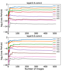
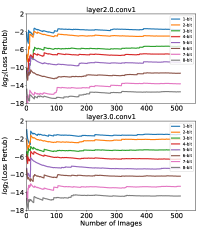
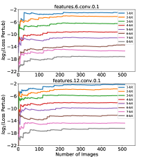
Convergence Analysis: As shown in Algorithm 1, we need to traverse the entire given training dataset for the calculation of loss perturbation $\Delta\mathcal{L}$. However, as the scale of the dataset increases, this calculation will become the bottleneck of time cost of the whole algorithm. Therefore, we first analyze the convergence of loss perturbation with regard to the number of images. As shown in Figure 1, the results converge rapidly with a few hundred images for all kinds of architectures, which indicates the chance to improve the algorithm’s efficiency significantly. Consequently, we only sample 1024 images randomly to figure out the loss perturbation in the following experiments.

Efficiency Analysis: Although most previous methods focus on performance improvement, we argue that computation efficiency should also be taken seriously in the actual deployment. For the search-based methods of AutoQ [26], it explores 400 episodes totally with the proposed hierarchical-DRL algorithm and fine-tunes each quantization policy with ten epochs in the randomly selected 100 categories of images from ImageNet for evaluation. In other words, it takes more than 1000 GPU-hours of RTX 2080Ti to search for the optimal bit-width of ResNet-50. And for the criterion-based methods of HAWQ-V2 [10], which is much more efficient, it still needs 30 minutes with 4 GPUs to calculate all the average Hessian traces of ResNet-50, let alone the time cost of the Pareto frontier calculation for automatic bit-width assignment. By contrast, thanks to the rapid convergence of loss perturbation and efficient greedy search algorithm, our method only takes less than 2 minutes to finish the whole bit-width assignment procedure of ResNet-50 with a single RTX 2080Ti and demonstrates significant efficiency advantage (see supplementary material for the theoretical analysis of computation complexity).

4.2 Ablation Study

In this section, we conduct ablation studies to justify the effectiveness of our method’s different parts.

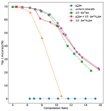
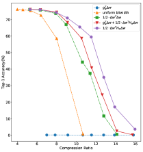
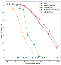
Approximated Hessian Matrix: As stated above, we adopt the approximated second-order term $\frac{1}{2}\Delta w^{T}\tilde{H}_{w}\Delta w$ as the proxy loss perturbation. To verify its advantages, we employ several other candidates for mixed-precision quantization and summarize the results in Figure 3. First, as the pre-trained model converges to a local minimum with nearly zero gradient vector, there is a devastating accuracy drop if only the first-order term is adopted. Second, compared with uniform bit-width and other Hessian-free (e.g. $\frac{1}{2}\Delta w^{T}\Delta w$) candidates, the significant performance improvement makes it worthwhile to pay for the extra computational cost of second-order information, especially for deep (e.g. ResNet-50) and lightweight (e.g. MobileNet-V2) networks. Finally, although it’s theoretically better to combine the first and second-order terms, our experimental results contradict this intuition. We believe that it’s because the extremely weak gradient information, which should be zero theoretically, acts more as noise for our loss perturbation approximation.

(a) ResNet-18

(b) ResNet-50

(c) Mobilenet-V2

Figure 3: Comparision of different loss perturbation approximations for bit-width assignment of various kinds of architectures.

(a) ResNet-18

(b) ResNet-50

(c) Mobilenet-V2

Figure 4: Bit-width assignment for various kinds of architectures.

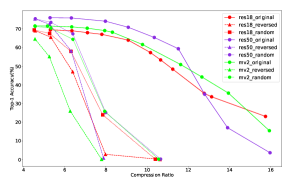
MCKP Reformulation: As MCKP is NP-hard, we propose a greedy search algorithm to solve it efficiently. To justify the effectiveness of the original criterion, we compare it with the other two ones, namely the reversed criterion and the random criterion. Specifically, the reversed criterion means that we choose the layer to increase bit-width with the lowest (instead of the highest) priority based on the original criterion, and the random criterion means that we choose the layer randomly. The results are summarized in Figure 2. As we can see, the original criterion outperforms the other two ones consistently for various kinds of architectures.

4.3 Comparision with SOTAs

Furthermore, we compare the accuracy results after fine-tuning with several quantization methods proposed recently, which including uniform and mixed-precision quantization. The summarized results are reported in Table 1(see supplementary material for the experimental setup).

For ResNet-18, compared with LQ-Nets [38] which introduces learnable scale factor for each bit, our method attains a smaller accuracy drop ($-0.26\%$ vs. $-0.30\%$) with larger compression ratio ($10.66\times$ vs. $6.10\times$). What’s more, under the setting that the compression ratio of both weights and activations $\geq 8.00\times$, we can achieve almost lossless accuracy ($0.10\%$ drop), which improves significantly against other uniform quantization methods.

For ResNet-50, except for uniform quantization, we also compare with other mixed-precision methods that including AutoQ [26], HAWQ [11], HAWQ-V2 [10], and HAQ [35]. Compared with HAWQ and HAWQ-V2 that also utilize the second-order information of the model, we achieve significantly less accuracy drop ($-0.85\%$ vs. $-1.91\%$) with a similar compression ratio. Compared with HAQ that leverages reinforcement learning to search for optimal bit-width assignment, our method reaches the same accuracy drop ($0.85\%$ drop) with a much larger compression ratio for both weights and activations and less computation cost.

Table 1: Summary of quantization results on ImageNet dataset. We compare with various kinds of uniform quantization methods such as DC [13], ABC-Net [22], LQ-Nets [38], DoReFa-Net [41] and PACT [7], and also recent mixed-precision methods such as AutoQ [26], HAWQ [11], HAWQ-V2 [10] and HAQ [35]. The ‘MP’ refers to mixed-precision quantization, where we report the lowest bits used for weights and activations. The ‘w-ratio’ and ‘a-ratio’ stand for weight and activation compression ratio, respectively.

[b] Network Method Top-1/Full w-bits a-bits w-ratio a-ratio Top-1/Quant Top-1/Drop ResNet-18 LQ-Nets^†  [38] $70.30$ $3$ $32$ $7.45\times$ $1.00\times$ $69.30$ $-1.00$ LQ-Nets^†  [38] $70.30$ $4$ $32$ $6.10\times$ $1.00\times$ $70.00$ $-0.30$ Ours $\bm{69.76}$ $\bm{2_{MP}}$ $\bm{32}$ $\bm{10.66\times}$ $\bm{1.00\times}$ $\bm{69.50}$ $\bm{-0.26}$ Ours $\bm{69.76}$ $\bm{2_{MP}}$ $\bm{8}$ $\bm{10.66\times}$ $\bm{4.00\times}$ $\bm{69.39}$ $\bm{-0.37}$ 2-9 ABC-Net [22] $69.30$ $5$ $5$ $6.40\times$ $6.40\times$ $65.00$ $-4.30$ LQ-Nets^†  [38] $70.30$ $4$ $4$ $6.10\times$ $7.98\times$ $69.30$ $-1.00$ DoReFa^†  [41] $70.40$ $5$ $5$ $5.16\times$ $6.39\times$ $68.40$ $-2.00$ PACT^†  [7] $70.40$ $4$ $4$ $6.10\times$ $7.98\times$ $69.20$ $-1.20$ Ours $\bm{69.76}$ $\bm{3_{MP}}$ $\bm{4_{MP}}$ $\bm{8.32\times}$ $\bm{8.00\times}$ $\bm{69.66}$ $\bm{-0.10}$ ResNet-50 ABC-Net [22] $76.10$ $5$ $5$ $6.40\times$ $6.40\times$ $70.10$ $-6.00$ LQ-Nets^†  [38] $76.40$ $3$ $3$ $5.99\times$ $10.64\times$ $74.20$ $-2.20$ LQ-Nets^†  [38] $76.40$ $4$ $4$ $5.11\times$ $7.99\times$ $75.10$ $-1.30$ DoReFa^†  [41] $76.90$ $4$ $4$ $5.11\times$ $7.99\times$ $71.40$ $-5.50$ PACT^†  [7] $76.90$ $32$ $4$ $1.00\times$ $7.99\times$ $75.90$ $-1.00$ PACT^†  [7] $76.90$ $2$ $4$ $7.24\times$ $7.99\times$ $74.50$ $-2.40$ AutoQ[26] $74.80$ $MP$ $MP$ $10.26\times$ $7.96\times$ $72.51$ $-2.29$ HAWQ[11] $77.39$ $2_{MP}$ $4_{MP}$ $12.28\times$ $8.00\times$ $75.48$ $-1.91$ HAWQ-V2[10] $77.39$ $2_{MP}$ $4_{MP}$ $12.24\times$ $8.00\times$ $75.76$ $-1.63$ HAQ[35] $76.15$ $MP$ $32$ $10.57\times$ $1.00\times$ $75.30$ $-0.85$ Ours $\bm{76.13}$ $\bm{2_{MP}}$ $\bm{4_{MP}}$ $\bm{12.24\times}$ $\bm{8.00\times}$ $\bm{75.28}$ $\bm{-0.85}$ MobileNet-V2 DC[13] $71.87$ $MP$ $32$ $13.93\times$ $1.00\times$ $58.07$ $-13.80$ HAQ[35] $71.87$ $MP$ $32$ $14.07\times$ $1.00\times$ $66.75$ $-5.12$ Ours $\bm{71.88}$ $\bm{2_{MP}}$ $\bm{8}$ $\bm{13.99\times}$ $\bm{4.00\times}$ $\bm{68.52}$ $\bm{-3.36}$ 2-9 DC[13] $71.87$ $MP$ $32$ $9.69\times$ $1.00\times$ $68.00$ $-3.87$ HAQ[35] $71.87$ $MP$ $32$ $9.69\times$ $1.00\times$ $70.90$ $-0.97$ Ours $\bm{71.88}$ $\bm{2_{MP}}$ $\bm{8}$ $\bm{9.79\times}$ $\bm{4.00\times}$ $\bm{71.20}$ $\bm{-0.68}$ 2-9 DC[13] $71.87$ $MP$ $32$ $7.47\times$ $1.00\times$ $71.24$ $-0.63$ HAQ[35] $71.87$ $MP$ $32$ $7.47\times$ $1.00\times$ $71.47$ $-0.40$ Ours $\bm{71.88}$ $\bm{3_{MP}}$ $\bm{8}$ $\bm{7.49\times}$ $\bm{4.00\times}$ $\bm{71.83}$ $\bm{-0.05}$

• do not quantize the first and last layer

At last, a much more efficient and lightweight architecture, MobileNet-V2, is utilized for further evaluation. Here we mainly compare with DC [8] and HAQ [35], which are uniform and mixed-precision quantization methods respectively. It should be noted that these two methods employ $k$-means algorithm to quantize the weights, and we instead adopt fixed-point quantization that sacrifices model accuracy for inference efficiency. Even under the situation of an unfair comparison, we still achieve significant performance improvement with a similar weight compression ratio and higher activation compression ratio in three different compression regimes, which justifies our method further.

4.4 Bit-width assignment

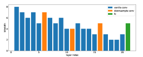
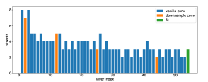
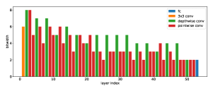
Finally, as shown in Figure 4, we visualize the bit-width assignment for these three networks to understand what our method learns. First, on ResNet-18 and ResNet-50, as the first convolution layer processes the input image directly and is much lighter than other layers, it receives a higher bit-width. Then, on ResNet-18, we notice that the output FC layer and downsample convolution layers also obtain higher bit-width, which is consistent with our prior knowledge that these components are critical for model performance. However, it should be noted that this conclusion does not hold strictly for ResNet-50, which is worthy of our further exploration. Besides, on MobileNet-V2, our method recognizes that depthwise convolution layers are more sensitive to quantization and allocates them higher bit-width, which is consistent with the conclusion of previous work[35].

5 Conclusion

In this paper, we present a novel and principled framework to solve the mixed-precision quantization problem. We first formulate the mixed-precision quantization as a discrete constrained optimization problem to provide a principled and holistic view. To solve the optimization problem, we propose an efficient approach to compute the Hessian matrix. Then we reformulate it as Multiple-Choice Knapsack Problem (MCKP) and propose a greedy search algorithm to solve it efficiently. Extensive experiments are conducted to demonstrate the efficiency and effectiveness of the proposed method over other uniform and mixed-precision quantization approaches.

References

- [1] Vijay Badrinarayanan, Alex Kendall, and Roberto Cipolla. Segnet: A deep convolutional encoder-decoder architecture for image segmentation. IEEE Trans. Pattern Anal. Mach. Intell., 39(12):2481--2495, 2017.
- [2] Yoshua Bengio, Nicholas Léonard, and Aaron C. Courville. Estimating or propagating gradients through stochastic neurons for conditional computation. CoRR, abs/1308.3432, 2013.
- [3] Zhaowei Cai, Xiaodong He, Jian Sun, and Nuno Vasconcelos. Deep learning with low precision by half-wave gaussian quantization. In 2017 IEEE Conference on Computer Vision and Pattern Recognition, CVPR 2017, Honolulu, HI, USA, July 21-26, 2017, pages 5406--5414, 2017.
- [4] Liang-Chieh Chen, George Papandreou, Iasonas Kokkinos, Kevin Murphy, and Alan L. Yuille. Deeplab: Semantic image segmentation with deep convolutional nets, atrous convolution, and fully connected crfs. IEEE Trans. Pattern Anal. Mach. Intell., 40(4):834--848, 2018.
- [5] Jian Cheng, Peisong Wang, Gang Li, Qinghao Hu, and Hanqing Lu. Recent advances in efficient computation of deep convolutional neural networks. Frontiers Inf. Technol. Electron. Eng., 19(1):64--77, 2018.
- [6] Yu Cheng, Duo Wang, Pan Zhou, and Tao Zhang. A survey of model compression and acceleration for deep neural networks. CoRR, abs/1710.09282, 2017.
- [7] Jungwook Choi, Zhuo Wang, Swagath Venkataramani, Pierce I-Jen Chuang, Vijayalakshmi Srinivasan, and Kailash Gopalakrishnan. PACT: parameterized clipping activation for quantized neural networks. CoRR, abs/1805.06085, 2018.
- [8] Lei Deng, Guoqi Li, Song Han, Luping Shi, and Yuan Xie. Model compression and hardware acceleration for neural networks: A comprehensive survey. Proc. IEEE, 108(4):485--532, 2020.
- [9] Emily L. Denton, Wojciech Zaremba, Joan Bruna, Yann LeCun, and Rob Fergus. Exploiting linear structure within convolutional networks for efficient evaluation. In Advances in Neural Information Processing Systems 27: Annual Conference on Neural Information Processing Systems 2014, December 8-13 2014, Montreal, Quebec, Canada, pages 1269--1277, 2014.
- [10] Zhen Dong, Zhewei Yao, Yaohui Cai, Daiyaan Arfeen, Amir Gholami, Michael W. Mahoney, and Kurt Keutzer. HAWQ-V2: hessian aware trace-weighted quantization of neural networks. CoRR, abs/1911.03852, 2019.
- [11] Zhen Dong, Zhewei Yao, Amir Gholami, Michael W. Mahoney, and Kurt Keutzer. HAWQ: hessian aware quantization of neural networks with mixed-precision. In 2019 IEEE/CVF International Conference on Computer Vision, ICCV 2019, Seoul, Korea (South), October 27 - November 2, 2019, pages 293--302, 2019.
- [12] Yunhui Guo. A survey on methods and theories of quantized neural networks. CoRR, abs/1808.04752, 2018.
- [13] Song Han, Huizi Mao, and William J. Dally. Deep compression: Compressing deep neural network with pruning, trained quantization and huffman coding. In 4th International Conference on Learning Representations, ICLR 2016, San Juan, Puerto Rico, May 2-4, 2016, Conference Track Proceedings, 2016.
- [14] Kaiming He, Xiangyu Zhang, Shaoqing Ren, and Jian Sun. Deep residual learning for image recognition. In 2016 IEEE Conference on Computer Vision and Pattern Recognition, CVPR 2016, Las Vegas, NV, USA, June 27-30, 2016, pages 770--778, 2016.
- [15] Geoffrey E. Hinton, Oriol Vinyals, and Jeffrey Dean. Distilling the knowledge in a neural network. CoRR, abs/1503.02531, 2015.
- [16] Benoit Jacob, Skirmantas Kligys, Bo Chen, Menglong Zhu, Matthew Tang, Andrew G. Howard, Hartwig Adam, and Dmitry Kalenichenko. Quantization and training of neural networks for efficient integer-arithmetic-only inference. In 2018 IEEE Conference on Computer Vision and Pattern Recognition, CVPR 2018, Salt Lake City, UT, USA, June 18-22, 2018, pages 2704--2713, 2018.
- [17] Hans Kellerer, Ulrich Pferschy, and David Pisinger. Knapsack problems. Springer, 2004.
- [18] Alex Krizhevsky, Ilya Sutskever, and Geoffrey E. Hinton. Imagenet classification with deep convolutional neural networks. In Advances in Neural Information Processing Systems 25: 26th Annual Conference on Neural Information Processing Systems 2012. Proceedings of a meeting held December 3-6, 2012, Lake Tahoe, Nevada, United States., pages 1106--1114, 2012.
- [19] Fengfu Li and Bin Liu. Ternary weight networks. CoRR, abs/1605.04711, 2016.
- [20] Hao Li, Asim Kadav, Igor Durdanovic, Hanan Samet, and Hans Peter Graf. Pruning filters for efficient convnets. In 5th International Conference on Learning Representations, ICLR 2017, Toulon, France, April 24-26, 2017, Conference Track Proceedings, 2017.
- [21] Tsung-Yi Lin, Piotr Dollár, Ross B. Girshick, Kaiming He, Bharath Hariharan, and Serge J. Belongie. Feature pyramid networks for object detection. In 2017 IEEE Conference on Computer Vision and Pattern Recognition, CVPR 2017, Honolulu, HI, USA, July 21-26, 2017, pages 936--944, 2017.
- [22] Xiaofan Lin, Cong Zhao, and Wei Pan. Towards accurate binary convolutional neural network. In Advances in Neural Information Processing Systems 30: Annual Conference on Neural Information Processing Systems 2017, 4-9 December 2017, Long Beach, CA, USA, pages 345--353, 2017.
- [23] Wei Liu, Dragomir Anguelov, Dumitru Erhan, Christian Szegedy, Scott E. Reed, Cheng-Yang Fu, and Alexander C. Berg. SSD: single shot multibox detector. In Computer Vision - ECCV 2016 - 14th European Conference, Amsterdam, The Netherlands, October 11-14, 2016, Proceedings, Part I, pages 21--37, 2016.
- [24] Zhuang Liu, Mingjie Sun, Tinghui Zhou, Gao Huang, and Trevor Darrell. Rethinking the value of network pruning. In 7th International Conference on Learning Representations, ICLR 2019, New Orleans, LA, USA, May 6-9, 2019, 2019.
- [25] Jonathan Long, Evan Shelhamer, and Trevor Darrell. Fully convolutional networks for semantic segmentation. In Proceedings of the IEEE conference on computer vision and pattern recognition, pages 3431--3440, 2015.
- [26] Qian Lou, Feng Guo, Minje Kim, Lantao Liu, and Lei Jiang. Autoq: Automated kernel-wise neural network quantization. In 8th International Conference on Learning Representations, ICLR 2020, Addis Ababa, Ethiopia, April 26-30, 2020, 2020.
- [27] Mohammad Rastegari, Vicente Ordonez, Joseph Redmon, and Ali Farhadi. Xnor-net: Imagenet classification using binary convolutional neural networks. In Computer Vision - ECCV 2016 - 14th European Conference, Amsterdam, The Netherlands, October 11-14, 2016, Proceedings, Part IV, pages 525--542, 2016.
- [28] Shaoqing Ren, Kaiming He, Ross B. Girshick, and Jian Sun. Faster R-CNN: towards real-time object detection with region proposal networks. In Advances in Neural Information Processing Systems 28: Annual Conference on Neural Information Processing Systems 2015, December 7-12, 2015, Montreal, Quebec, Canada, pages 91--99, 2015.
- [29] Adriana Romero, Nicolas Ballas, Samira Ebrahimi Kahou, Antoine Chassang, Carlo Gatta, and Yoshua Bengio. Fitnets: Hints for thin deep nets. In 3rd International Conference on Learning Representations, ICLR 2015, San Diego, CA, USA, May 7-9, 2015, Conference Track Proceedings, 2015.
- [30] Hardik Sharma, Jongse Park, Naveen Suda, Liangzhen Lai, Benson Chau, Vikas Chandra, and Hadi Esmaeilzadeh. Bit fusion: Bit-level dynamically composable architecture for accelerating deep neural network. In 45th ACM/IEEE Annual International Symposium on Computer Architecture, ISCA 2018, Los Angeles, CA, USA, June 1-6, 2018, pages 764--775, 2018.
- [31] Karen Simonyan and Andrew Zisserman. Very deep convolutional networks for large-scale image recognition. CoRR, abs/1409.1556, 2014.
- [32] Vivienne Sze, Yu-Hsin Chen, Tien-Ju Yang, and Joel S. Emer. Efficient processing of deep neural networks: A tutorial and survey. Proc. IEEE, 105(12):2295--2329, 2017.
- [33] Stefan Uhlich, Lukas Mauch, Fabien Cardinaux, Kazuki Yoshiyama, Javier Alonso García, Stephen Tiedemann, Thomas Kemp, and Akira Nakamura. Mixed precision dnns: All you need is a good parametrization. In 8th International Conference on Learning Representations, ICLR 2020, Addis Ababa, Ethiopia, April 26-30, 2020, 2020.
- [34] Yaman Umuroglu, Lahiru Rasnayake, and Magnus Själander. BISMO: A scalable bit-serial matrix multiplication overlay for reconfigurable computing. In 28th International Conference on Field Programmable Logic and Applications, FPL 2018, Dublin, Ireland, August 27-31, 2018, pages 307--314, 2018.
- [35] Kuan Wang, Zhijian Liu, Yujun Lin, Ji Lin, and Song Han. HAQ: hardware-aware automated quantization with mixed precision. In IEEE Conference on Computer Vision and Pattern Recognition, CVPR 2019, Long Beach, CA, USA, June 16-20, 2019, pages 8612--8620, 2019.
- [36] Bichen Wu, Yanghan Wang, Peizhao Zhang, Yuandong Tian, Peter Vajda, and Kurt Keutzer. Mixed precision quantization of convnets via differentiable neural architecture search. CoRR, abs/1812.00090, 2018.
- [37] Yong Yuan, Chen Chen, Xiyuan Hu, and Silong Peng. Evoq: Mixed precision quantization of dnns via sensitivity guided evolutionary search. In 2020 International Joint Conference on Neural Networks, IJCNN 2020, Glasgow, United Kingdom, July 19-24, 2020, pages 1--8, 2020.
- [38] Dongqing Zhang, Jiaolong Yang, Dongqiangzi Ye, and Gang Hua. Lq-nets: Learned quantization for highly accurate and compact deep neural networks. In Computer Vision - ECCV 2018 - 15th European Conference, Munich, Germany, September 8-14, 2018, Proceedings, Part VIII, pages 373--390, 2018.
- [39] Xiangyu Zhang, Jianhua Zou, Kaiming He, and Jian Sun. Accelerating very deep convolutional networks for classification and detection. IEEE Trans. Pattern Anal. Mach. Intell., 38(10):1943--1955, 2016.
- [40] Aojun Zhou, Anbang Yao, Yiwen Guo, Lin Xu, and Yurong Chen. Incremental network quantization: Towards lossless cnns with low-precision weights. In 5th International Conference on Learning Representations, ICLR 2017, Toulon, France, April 24-26, 2017, Conference Track Proceedings, 2017.
- [41] Shuchang Zhou, Zekun Ni, Xinyu Zhou, He Wen, Yuxin Wu, and Yuheng Zou. Dorefa-net: Training low bitwidth convolutional neural networks with low bitwidth gradients. CoRR, abs/1606.06160, 2016.
- [42] Chenzhuo Zhu, Song Han, Huizi Mao, and William J. Dally. Trained ternary quantization. In 5th International Conference on Learning Representations, ICLR 2017, Toulon, France, April 24-26, 2017, Conference Track Proceedings, 2017.