Rotation acceleration of asteroids (10115) 1992 SK, (1685) Toro, and (1620) Geographos due to the YORP effect

Abstract

Context. The rotation state of small asteroids is affected by the Yarkovsky–O’Keefe–Radzievskii–Paddack (YORP) effect, which is a net torque caused by solar radiation directly reflected and thermally reemitted from the surface. Due to this effect, the rotation period slowly changes, which can be most easily measured in light curves because the shift in the rotation phase accumulates over time quadratically.

Aims. By new photometric observations of selected near-Earth asteroids, we want to enlarge the sample of asteroids with a detected YORP effect.

Methods. We collected archived light curves and carried out new photometric observations for asteroids (10115) 1992 SK, (1620) Geographos, and (1685) Toro. We applied the method of light curve inversion to fit observations with a convex shape model. The YORP effect was modeled as a linear change of the rotation frequency $\upsilon\equiv\mathrm{d}\omega/\mathrm{d}t$ and optimized together with other spin and shape parameters.

Results. We detected the acceleration $\upsilon=(8.3\pm 0.6)\times 10^{-8}\,\text{rad}\,\text{d}^{-2}$ of the rotation for asteroid (10115) 1992 SK. This observed value agrees well with the theoretical value of YORP-induced spin-up computed for our shape and spin model. For (1685) Toro, we obtained $\upsilon=(3.3\pm 0.3)\times 10^{-9}\,\text{rad}\,\text{d}^{-2}$, which confirms an earlier tentative YORP detection. For (1620) Geographos, we confirmed the previously detected YORP acceleration and derived an updated value of $\upsilon$ with a smaller uncertainty. We also included the effect of solar precession into our inversion algorithm, and we show that there are hints of this effect in Geographos’ data.

Conclusions. The detected change of the spin rate of (10115) 1992 SK has increased the total number of asteroids with YORP detection to ten. In all ten cases, the $\mathrm{d}\omega/\mathrm{d}t$ value is positive, so the rotation of these asteroids is accelerated. It is unlikely to be just a statistical fluke, but it is probably a real feature that needs to be explained.

1 Introduction

The importance of nongravitational radiation forces for spin evolution of asteroids was fully recognized by Rubincam (2000), who coined the term Yarkovsky–O’Keefe–Radzievskii–Paddack (YORP) effect for solar radiation-induced torque that affects the rotation state of asteroids. The YORP effect is important for the evolution of the asteroid population, as asteroids can be accelerated to the rotation break limit, they can shed mass and create asteroid pairs or binaries. It also affects the distribution of rotation rates and obliquities in general. For details and further references, see the review of Vokrouhlický et al. (2015).

Research on theoretical aspects of YORP (Breiter et al., 2007; Nesvorný & Vokrouhlický, 2007; Breiter & Vokrouhlický, 2011; Rozitis & Green, 2012, for example) went hand in hand with efforts to detect this effect directly as a change in the rotation period (Kaasalainen et al., 2007; Lowry et al., 2007; Taylor et al., 2007). With the new YORP detections presented in this paper, the number of asteroids known to change their rotation period due to YORP has grown to ten, all of them being small near-Earth asteroids because the magnitude of the YORP effect is inversely proportional to the squared heliocentric distance and squared size. After five asteroids listed in the review of Vokrouhlický et al. (2015), there were four more: (161989) Cacus and (1865) Toro (only tentative detection, now confirmed in our paper) in Ďurech et al. (2018b), (101955) Bennu (Nolan et al., 2019; Hergenrother et al., 2019), and (68346) 2001 KZ66 (Zegmott et al., 2021). To these nine, we added the tenth detection of the rotation period change for asteroid (10115) 1992 SK. This, as all previous detections, also has a positive sign of $\mathrm{d}\omega/\mathrm{d}t$, so its rotation is accelerated.

2 Reconstructing the spin state and shape from light curves

To detect changes in the rotation periods that are too small to be found directly (as in the case of the asteroid YORP, Lowry et al., 2007), it is necessary to look for shifts in the rotation phase. Contrary to the rotation period, which evolves linearly when affected by YORP, the rotation phase drift accumulates over time and increases quadratically with time. We used the same approach as in Kaasalainen et al. (2007) or Ďurech et al. (2018a) – the change in the rotation rate $\omega$ is described by a free parameter $\upsilon\equiv\mathrm{d}\omega/\mathrm{d}t$ that is optimized during the light curve inversion together with the shape and spin parameters. If a nonzero $\upsilon$ provides a significantly better fit than $\upsilon=0$, we interpret it as detecting rotation acceleration or deceleration. The next step is to show that this observed value of $\upsilon$ is consistent with the YORP value predicted theoretically from the known shape, size, and spin of the asteroid (see Sect. 4). The light curve inversion method iteratively converges to best-fit parameters that minimize the difference between the observed and modeled light curves; this difference is measured by the standard $\chi^{2}$. To realistically estimate uncertainties of photometric data, we fit each light curve by a Fourier series of maximum order determined by an F-test (Magnusson et al., 1996). The root-mean-square residual was used as the uncertainty of individual light curve points. In other words, light curves were weighted according to their precision.

In the following subsections, we present spin parameters (listed also in Table 1) obtained as best-fit parameters by light curve inversion (Kaasalainen et al., 2001). Their uncertainties were estimated by a bootstrap method. For each asteroid we analyzed, we created 10,000 bootstrapped light curve data sets by randomly selecting a new set of light curves with a random resampling of light curve points. For each new data set, we repeated the inversion and obtained spin parameters. From the distribution of these parameters, we estimated their uncertainties. We also estimated the uncertainty of the $\upsilon$ parameter by varying it around its best value and looking at the increase in $\chi^{2}$. Error intervals provided by this approach are slightly larger than those determined by bootstrap for (10115) and Geographos and twice as large for Toro (see the Appendix for details).

2.1 (10115) 1992 SK

The first light curves of this asteroid were observed in 1999, and they were used together with radar delay-Doppler observations for the shape reconstruction by Busch et al. (2006). Other photometry comes from 2006 (Polishook, 2012) and 2013 (Warner, 2014). We observed this object during two apparitions in 2017 and 2020. Using these calibrated observations and also those from February to March 1999, we determined its mean absolute magnitude $H=17.31\pm 0.18$ mag, assuming the slope parameter $G=0.24\pm 0.11$ (which is the $1\sigma$ range of G values for S type asteroids from Warner et al., 2009). The color index in the Johnson-Cousins system is $V-R=0.458\pm 0.013$ mag, consistent with its Sq/S spectral classification of Thomas et al. (2014) and Binzel et al. (2019). All available light curves are listed in Table C.

The light curve inversion provided unambiguous results; the detection of the period change is robust, that is, a model with a constant rotation period provides a significantly worse fit to light curves than the YORP model. The best-fit model has a pole direction in ecliptic coordinates $(94^{\circ},-56^{\circ})$, the rotation period $P=7.320232\pm 0.000010$ h (for JD 2451192.0), and the YORP value $\upsilon=(8.3\pm 0.6)\times 10^{-8}\,\text{rad}\,\text{d}^{-2}$ ($1\sigma$ errors). The shape model is shown in Fig. 1 and the agreement between synthetic light curves produced by this shape and real observations is demonstrated in Fig. 2. The distribution of bootstrap results for the spin axis direction was bi-modal with $\lambda$ in the range 90–120^∘ and $\beta$ between $-65$ and $-45^{\circ}$ (see Fig. 3). Formal $1\sigma$ uncertainties computed as standard deviations were $\pm 10^{\circ}$ for $\lambda$ and $\pm 5^{\circ}$ for $\beta$. The bi-modality is caused by the random selection of light curves in bootstrap and the importance of some light curves – the cloud of points around the pole direction $(110^{\circ},-60^{\circ})$ are mainly those solutions that do not have the light curve from 2020 December 4 in the bootstrap input data. Random resampling also causes the best-fit pole direction based on the original light curve data set to not be exactly at the position where the density of bootstrap solutions is the highest.

The radar-based model of Busch et al. (2006) has a similar shape as our convex model and a similar rotation period of $7.3182\pm 0.0003$ h (although the periods are different when measured by their $3\sigma$ uncertainty intervals), but its spin axis orientation $(99^{\circ},-3^{\circ})$ is significantly different from our value. Their model is not consistent with new light curves from 2017 – the light curve amplitudes are not correctly reproduced (see Fig. 2).

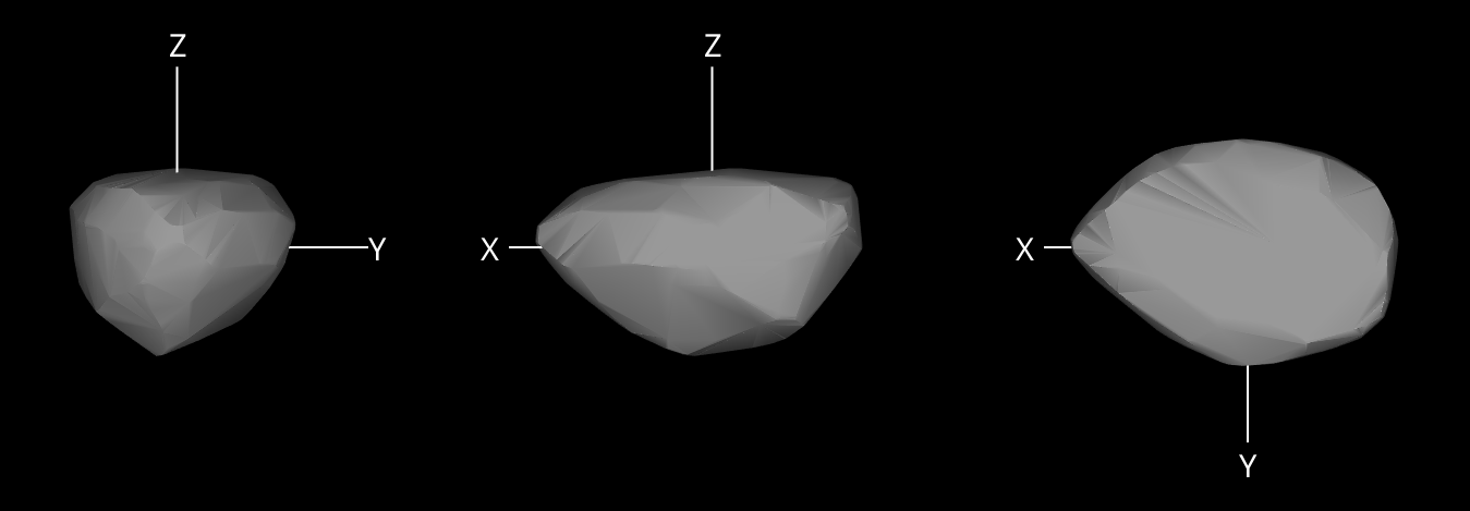
Figure 1: Shape model of asteroid (10115) 1992 SK shown from equatorial level (left and center, $90\degr$ apart) and pole-on (right).

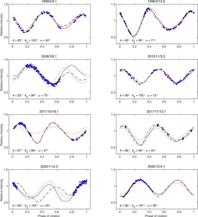
Figure 2: Example light curves (blue dots) of (10115) 1992 SK shown with the synthetic light curves produced by the best YORP model (red curves) and the best constant-period model (black dashed curves). We also show synthetic light curves generated by the shape and spin model of Busch et al. (2006) (dotted black curves). The latter were manually shifted in phase to give the best fit with observed data, but still, their amplitude is not consistent with 2017 observations. The geometry of the observation is described by the aspect angle $\theta$, the solar aspect angle $\theta_{0}$, and the solar phase angle $\alpha$.

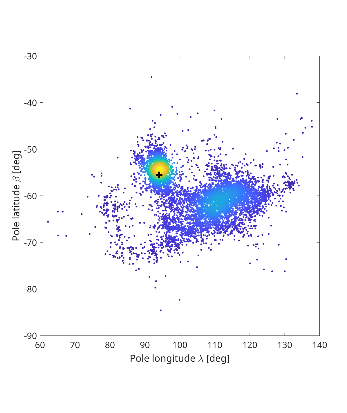
Figure 3: Direction of the spin axis in ecliptic coordinates $(\lambda,\beta)$ for 10,000 bootstrap models of (10115) 1992 SK. The density of points is color-coded, with the red color corresponding to the highest density. The black cross at $(95^{\circ},-54^{\circ})$ marks the spin-axis direction of the nominal model derived from the original light curve data set.

2.2 (1620) Geographos

There are a lot of photometric observations of Geographos going back to 1969. Geographos was also observed by radar and a shape model was reconstructed (Hudson & Ostro, 1999) and thermohpysical analysis was performed by Rozitis & Green (2014). YORP-induced acceleration of its rotation was detected by Ďurech et al. (2008a) by the inversion of light curves from 1969 to 2008. The rotation parameters were determined to ($3\sigma$ uncertainties): $\lambda=58\pm 6^{\circ}$, $\beta=-49\pm 7^{\circ}$, $P=5.223336\pm 0.000002$ h, and $\upsilon=(1.15\pm 0.15)\times 10^{-8}\,\text{rad\,d}^{-2}$.

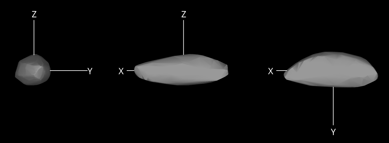
Figure 9: Shape model of asteroid (1620) Geographos shown from equatorial level (left and center, $90\degr$ apart) and pole-on (right).

We complemented the previous data set with new photometry from 2008, 2011, 2012, 2015, and 2019 (see Table C) and updated the spin parameters to the following new values ($1\sigma$ uncertainties): $\upsilon=(1.14\pm 0.03)\times 10^{-8}\,\text{rad}\,\text{d}^{-2}$ with period $P=5.2233360\pm 0.0000006\,\text{h}$ (for JD 2440229.0). The pole direction $\lambda=56.7\pm 0.7^{\circ}$, $\beta=-51.2\pm 1.1^{\circ}$ in ecliptic coordinates. The shape model is shown in Fig. 9.

2.3 (1685) Toro

A tentative YORP detection by Ďurech et al. (2018b) was based on a data set from apparitions in 1972 to 2016. To this, we added new observations from 2018, 2020, and 2021 (see Table C). We determined Toro’s mean absolute magnitude to $H=14.48\pm 0.13$ mag, assuming the slope parameter $G=0.24\pm 0.11$ (Warner et al., 2009). We measured the color index in the Johnson-Cousins system as $V-R=0.462\pm 0.010$ mag, which is consistent with its Sq/S spectral classification of Thomas et al. (2014) and Binzel et al. (2019).

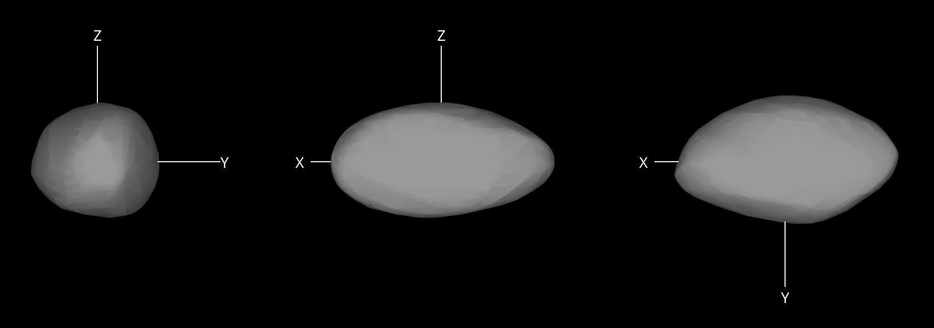
Figure 10: Shape model of asteroid (1685) Toro shown from equatorial level (left and center, $90\degr$ apart) and pole-on (right).

Previous values ($3\sigma$ errors) published by Ďurech et al. (2018b) were $P=10.19782\pm 0.00003\,$h, $(\lambda,\beta)=(71\pm 10^{\circ},-69\pm 5^{\circ})$, and $\upsilon=3.0\times 10^{-9}\text{rad\,d}^{-2}$. The updated values ($1\sigma$ errors) are as follows: $\upsilon=(3.3\pm 0.3)\times 10^{-9}\,\text{rad}\,\text{d}^{-2}$, $P=10.197826\pm 0.000002\,\text{h}$ (for JD 2441507.0). The pole direction is $(75\pm 3^{\circ},-69\pm 1^{\circ})$. The shape model is shown in Fig. 10. Although the model with YORP is significantly better than a constant-period model statistically, the difference between the synthetic light curves they produce is so small that they look almost the same when plotted on top of each other. In Fig. 4, we show four light curves for which the difference between the two models is the largest.

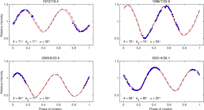
Figure 4: Example light curves (blue dots) of (1685) Toro shown with the synthetic light curves produced by the best YORP model (red curves) and the best constant-period model (black dashed curves). The geometry of observation is described by the aspect angle $\theta$, the solar aspect angle $\theta_{0}$, and the solar phase angle $\alpha$.

Table 1: Parameters derived from photometric data: Spin axis direction in ecliptic longitude $\lambda_{\text{p}}$ and latitude $\beta_{\text{p}}$, the sidereal rotation period $P$ at epoch JD₀, the YORP parameter $\upsilon$, the absolute magnitude $H$, and the color index $V-R$. The volume-equivalent diameters $D$ were taken from Hudson & Ostro (1999) for Geographos, from Ďurech et al. (2018b) for Toro, and from Busch et al. (2006) for 1999 SK.

Asteroid		$\lambda_{\text{p}}$	$\beta_{\text{p}}$	$P$	JD0	$\upsilon$	$D$	$H$	$V-R$
		[deg]	[deg]	[h]		[$\times 10^{-8}\,\text{rad}\,\text{d}^{-2}$]	[km]	[mag]	[mag]
(1620)	Geographos	$56.7\pm 0.7$	$-51.2\pm 1.1$	$5.2233360$	2440229.0	$1.14\pm 0.03$	$2.56\pm 0.15$
				$\pm 0.0000006$
(1685)	Toro	$75\pm 3$	$-69\pm 1$	$10.197826$	2441507.0	$0.33\pm 0.03$	$3.5^{+0.3}_{-0.4}$	$14.48\pm 0.13$	$0.462\pm 0.010$
				$\pm 0.000002$
(10115)	1992 SK	$94\pm 10$	$-56\pm 5$	$7.320232$	2451192.0	$8.3\pm 0.6$	$1.0\pm 0.2$	$17.31\pm 0.18$	$0.458\pm 0.013$
				$\pm 0.000010$

3 Solar torque precession

The detection of small secular changes on the order of $\mathrm{d}P/\mathrm{d}t\sim 10^{-11}$ to $10^{-9}$ in the rotation period is possible due to the long time span of photometric observations. In the case of Geographos, the data cover 50 years, and the large amplitude of its light curves enabled us to determine the rotation period and its secular change very precisely. For the same reasons, the spin axis’ direction was determined with an exquisite precision of about $1^{\circ}$.

So far, all light curve inversion models have assumed that the rotation axis is fixed in the inertial frame, which was a valid assumption for asteroids in principal axis rotation. Apart from changing the angular frequency, the YORP effect also causes a secular evolution of the spin axis obliquity, but this effect is so tiny that it is unobservable with current data sets. For example, the theoretical change in Geographos’ obliquity is smaller than one arcminute in 50 yr. However, there is another effect – a regular precession due to the solar gravitation torque – that inevitably affects the direction of the spin axis of all asteroids.

Solar gravitation torque acts on a rotating body and causes a secular precession of its rotation axis around the normal to its orbital plane. The precession constant $\alpha$ describes the angular velocity of the spin axis at the limit of zero obliquity and can be expressed as

$$\alpha=\frac{3n^{2}\Delta}{2\omega\eta^{3}}\,,$$ (1)

where $\eta$ is determined from eccentricity $e$ as $\eta=\sqrt{1-e^{2}}$, $\Delta$ is the dynamical ellipticity computed from the principal values of the inertia tensor $A,B,C$ as $1-0.5(A+B)/C$, $\omega$ is the angular rotational velocity $\omega=2\pi/P$, and $n$ is the orbital mean motion (e.g, Bertotti et al., 2003, chapter 4). If we substitute the values $\Delta=0.29\pm 0.02$ for Toro and $\Delta=0.407\pm 0.006$ for Geographos (uncertainties estimated by bootstrap), we get $\alpha=(356\pm 27)\arcsec/\text{yr}$ and $(289\pm 4)\arcsec/\text{yr}$, respectively. This formally accumulates to $\sim 4^{\circ}$ over 50 years. The motion of the rotation axis on the precession cone with obliquity $\epsilon$ has angular velocity $\Delta\varphi/\Delta t=\alpha\,\cos\epsilon$ and mainly affects the ecliptic longitude $\lambda$ of the spin axis for orbits of a moderately small inclination (see the next subsection). Even though the $\cos\epsilon$ factor slightly decreases the above-estimated effect, the formal uncertainty of the pole determination for Geographos is so small that precession should have a measurable effect on its photometric data.

3.1 Model of solar precession

We included solar precession in the light curve inversion algorithm to see if it somehow affects our results. The evolution of the unit spin vector $\@vec{s}(t)$ over small time interval $\Delta t$ is described as $\@vec{s}(t+\Delta t)=\@vec{s}(t)+\Delta\@vec{s}(t)$, where the incremental change $\Delta\@vec{s}=-(\@vec{N}\times\@vec{s})\,\Delta\varphi$. The normal to the orbital plane $\@vec{N}$ is defined by means of the inclination $i$ of the orbital plane to the ecliptic and the longitude of the ascending node $\Omega$ as: $\@vec{N}=(\sin i\sin\Omega;-\sin i\cos\Omega;\cos i)^{\text{T}}$. We assume that $i$ is constant and that $\Omega$ evolves linearly in time as $\Omega=\Omega_{0}+\dot{\Omega}t$. We took the values of $\dot{\Omega}$ from the NEODyS page, but the results with a constant $\Omega$ were practically the same because $\dot{\Omega}$ is an order of magnitude smaller than $\alpha$. The real angular shift $\Delta\varphi$ of the spin vector is $\Delta\varphi=\alpha\cos\epsilon\,\Delta t=\alpha\,(\@vec{s}\cdot\@vec{N})\,\Delta t$.

The initial (at the epoch of the first light curve) orientation of the spin vector $\@vec{s}_{0}$ is described by the ecliptic coordinates $\lambda_{0}$ and $\beta_{0}$, both being free parameters of optimization. Contrary to the standard light curve inversion, the pole direction is not fixed in space but evolves due to precession according to the equations given above.

For Geographos, the precession constant is $\alpha=289\,\arcsec/\text{yr}$, which implies the accumulated shift $\Delta\varphi=-3.54^{\circ}$ over 50 years. The corresponding change of ecliptic coordinates of the spin axis is $\Delta\lambda=2.44^{\circ}$ and $\Delta\beta=0.13^{\circ}$. This expected shift of the ecliptic longitude $\lambda$ is larger than its formal uncertainty of $0.7^{\circ}$ (Sect. 2.2), so precession should have a measurable effect on Geographos’ light curves. Indeed, including the evolution of $\@vec{s}$ into the inversion has a small, yet statistically significant effect on the goodness of the fit. We changed the precession constant $\alpha$ on the interval from $-1000$ to $1000\arcsec/\text{yr}$ with a step of $20\arcsec/\text{yr}$, and for each value, we repeated the light curve inversion, that is to say we optimized all shape and spin parameters, also including the YORP parameter $\upsilon$. The results are shown in Fig. 5, where $\chi^{2}$ values are plotted for different values of $\alpha$. Values of $\chi^{2}$ were rescaled such that the minimum value was equal to one. We can see a clear asymmetry with respect to zero precession – the lowest $\chi^{2}$ is obtained for $\alpha$ around 200–600 ″/yr. Without any precession ($\alpha=0$), the $\chi^{2}$ is about 0.5% higher than the minimum value, which is just a small increase, but still statistically significant given the number of data points (8852 in total). Moreover, the best fit is obtained for values of $\alpha$ that agree with the theoretical value of $\sim 300\arcsec/\text{yr}$, so we interpret this as a detection of the precession of the Geographos’ rotation axis due to the solar torque.

For Toro, the length of the time interval covered by observations (48 years, 6995 data points) is about the same as for Geographos; the precession constant $\alpha$ is similar, so the precession evolution is about the same: $\Delta\varphi=-4.36^{\circ}$, $\Delta\lambda=3.64^{\circ}$, and $\Delta\beta=-0.66^{\circ}$. However, the spin axis direction is not so tightly constrained, and including the parameter $\alpha$ into the model has a much smaller effect than in the case of Geographos. The dependence of $\chi^{2}$ on $\alpha$ is much weaker (Fig. 5). Although the $\chi^{2}$ versus $\alpha$ curve is also not symmetric around zero and positive values of $\alpha$ are preferred (the best fit is obtained for $\alpha\sim 400$–$900\,\arcsec/\text{yr}$), it is not robust with respect to the data set – that is, excluding some light curves from the data set or changing their formal errors has a strong effect on the shape of the $\alpha$ versus $\chi^{2}$ dependence. We repeated the $\alpha$ scan with bootstrapped light curve samples and confirmed that for Geographos, the results were much more stable than for Toro. From the sample of one hundred bootstrap repetitions, the value of $\alpha$ for which $\chi^{2}$ was minimal was $(330\pm 360)\,\arcsec/\text{yr}$ for Geographos, while for Toro it was $(-110\pm 620)\,\arcsec/\text{yr}$.

The dynamical ellipticity of asteroid 1992 SK is $\Delta=0.29$, which leads to theoretical $\alpha=283\,\arcsec/\text{yr}$. Accumulated over 22 years of observations, $\Delta\varphi=-1.56^{\circ}$, which is too small given the large uncertainties of the pole direction – thus this effect is not detectable with the current data set.

Geographos and Toro are almost ideal candidates for the search of the effect of precession on photometric data – they are near-Earth asteroids (large $n$), elongated (large $\Delta$), and not rotating too quickly (low $\omega$). It is not likely that many asteroids will have $\alpha$ much larger than a couple of hundreds of arcsec per year. From the modeling point of view, precession will continue to be negligible for most of the asteroids. However, for slowly rotating elongated near-Earth asteroids with suitable obliquity and observations covering many decades, this effect will become measurable and should be included in the modeling. In principle, the precession rate $\alpha$ can be treated as another free parameter of the light curve fitting procedure, so $\Delta$ can be determined (Eq. 1) from observations independently of the shape model. Its value may then be compared with that computed from the shape model assuming a uniform density distribution.

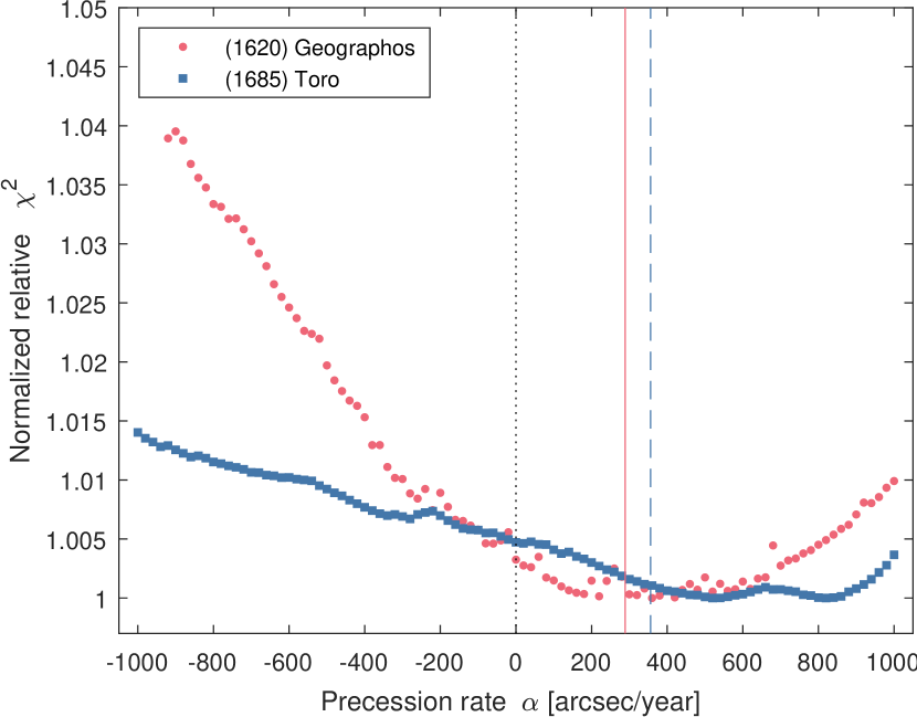
Figure 5: Normalized relative $\chi^{2}$ versus precession rate $\alpha$ for (1620) Geographos and (1685) Toro. The nominal values of $\alpha=289\arcsec/\text{yr}$ for Geographos (solid) and $\alpha=356\arcsec/\text{yr}$ for Toro (dashed) are marked with vertical lines. The iterative convergence of the inversion algorithm is not ideal and causes some scatter of points mainly on Geographos’ curve.

4 Comparison of the detected $\upsilon$ values with the theoretical model

A secular change in the rotation rate of the three objects presented in Sec. 2 has been obtained using a fully empirical approach, namely by adjusting the rate factor $\upsilon=\mathrm{d}\omega/\mathrm{d}t$ to match the observations. In order to physically interpret $\upsilon$, it is now important to compare it with a model prediction. We postulate that the YORP effect is the underlying mechanism that makes the rotation rate of (10115) 1992 SK, (1685) Toro, and (1620) Geographos accelerate, and we therefore use a model description of YORP to predict the expected level of $\upsilon_{\rm mod}$. A comparison between $\upsilon$ and $\upsilon_{\rm mod}$ helps to verify, or reject, our assumption, and eventually argue about parameters on which $\upsilon_{\rm mod}$ depends. A well-known issue with the YORP model exists because (i) some of its free parameters are apparent from the observations, such as the rotation state or size, (ii) some may be plausibly expected and described by a reliable statistical distribution, such as the bulk density, but (iii) some others cannot be easily described or determined. This last class depends on the small-scale irregularities of the asteroid shape. Yet, numerical tests confirmed that $\upsilon_{\rm mod}$ may in some circumstances strongly depend on this last class of parameters (e.g., Statler, 2009; Rozitis & Green, 2012, 2013a; Golubov & Krugly, 2012).

With this caveat in mind, we used a fully thermophysical model of Čapek & Vokrouhlický (2004), see also Čapek & Vokrouhlický (2005), to evaluate the surface temperature on a body, whose shape is represented with a general polyhedron. The number of surface facets $N$, provided by inversion of the photometric observations, is typically a couple thousand. As a rule of thumb, this allows one to resolve surface features of a characteristic scale $\propto D\,\sqrt{\pi/N}$, that is, some $\simeq 40$ meters at best for kilometer-sized asteroids. Our approach treats each of the surface facets individually and solves the one-dimensional problem of heat conduction below the surface. A fixed configuration of the heliocentric orbit and rotation pole of the body is assumed. Boundary conditions express (i) energy conservation at the surface (with solar radiation as an external source) and (ii) a constant temperature at great depth (implying an isothermal core of the body). Given a plausible range of surface thermal conductivity values and typical rotation rates of asteroids, the penetration depth of a thermal wave is in the centimeter to meter range. With the coarse resolution of the shape model, the one-dimensional treatment of the problem is justified. The model, in principle, accounts for mutual shadowing of surface units, but neglects their mutual irradiation (e.g., Rozitis & Green, 2012) and possible thermal communication via conduction (which would require a resolution model at the level of penetration depth of the thermal wave, e.g., Golubov & Krugly, 2012). We also assume simple Lambertian thermal emission from the surface, neglecting thermal beaming related again to the small-scale surface roughness (e.g., Rozitis & Green, 2013a). All these complications must be accounted for with an empirical correction. Once the surface temperature was determined for any of the surface facets, and at any moment during the revolution about the Sun, the thermal recoil force and torque were determined (in the torque part, we also added effects of the directly reflected sunlight in the optical waveband). The force part may help to determine the orbit-averaged change $\mathrm{d}a/\mathrm{d}t$ of the heliocentric semimajor axis (the Yarkovsky effect), and the torque provides the orbit-averaged change $\upsilon=\mathrm{d}\omega/\mathrm{d}t$ of the rotation rate (the YORP effect). Technical details may be found in the abovementioned papers by Čapek & Vokrouhlický (2004) and Čapek & Vokrouhlický (2005).

In our simulations, we tested surface thermal conductivity values in the range of $40$ to nearly $1200$ J m^-1 K^-1 s^-1/2 which are appropriate for kilometer-sized near-Earth asteroids (e.g., Delbò et al., 2015). All three asteroids discussed in Sec. 2 are spectrally S-type. This justifies our nominal choice of the bulk density $\rho=2.5$ g cm^-3, though slightly larger values have been determined for larger asteroids, while possibly smaller values for small near-Earth objects (see, e.g., Scheeres et al., 2015). A realistic uncertainty in the adopted bulk density may, therefore, be $\simeq 0.7$ g cm^-3. Parameters of the rotation state, namely the rotation period and pole, were taken from our solution in Sec. 2, and the parameters of heliocentric orbits from standard databases (such as JPL or AstDyS).

4.1 (10115) 1992 SK

Using the physical parameters mentioned above and scaling our convex-shape model such that it has a volume equivalent to a sphere of diameter $1$ km (Busch et al., 2006), we obtained $\upsilon_{\rm mod}=19.3\times 10^{-8}$ rad d^-2 by YORP. As already found by Čapek & Vokrouhlický (2004), and later verified by both numerical and analytical means (e.g., Vokrouhlický et al., 2015, and references therein), the predicted $\upsilon_{\rm mod}$ does not depend on the surface thermal conductivity in the simple one-dimensional heat conduction approach used. So our predicted value potentially rescales only with adjustments to the size $D$ and bulk density $\rho$ with $\upsilon_{\rm mod}\propto 1/(\rho D^{2})$. Nonetheless, the difference between our base value of $\upsilon_{\rm mod}$ and the observed $\upsilon=(8.3\pm 0.6)\times 10^{-8}$ rad d^-2 is comfortably small, in fact smaller than in some other cases of asteroids with YORP detections. Additionally, it can be made closer to the observed value by (i) a plausible small increase in the bulk density and/or size, or (ii) by accounting for beaming and self-heating phenomena in the YORP computation (e.g., Rozitis & Green, 2012, 2013a). We note that the latter effects tend to decrease the predicted $\upsilon_{\rm mod}$ value, suitably approaching the observed value. On the other hand, effects of the lateral heat conduction in centimeter- to decimeter-sized surface irregularities would produce an additional acceleration component in $\upsilon_{\rm mod}$ (e.g., Golubov & Krugly, 2012). Since this component is not significantly apparent, we assume the surface of (10115) 1992 SK is not overly rugged. This is also in agreement with conclusions driven from the analysis of radar data by Busch et al. (2006), who interpreted the radar circular polarization measurements as an indication of a similarity to the surface of Eros.

Our runs also provide the predicted value of the Yarkovsky effect, namely a rate of secular change in the semimajor axis. For the abovementioned nominal values of physical parameters, and the rotation state determined in Sec. 2, we find that $(\mathrm{d}a/\mathrm{d}t)_{\rm mod}$ ranges between $-1.5\times 10^{-4}$ and $-4\times 10^{-4}$ au Myr^-1, with a maximum value for the surface thermal inertia $\simeq 260$ J m^-1 K^-1 s^-1/2 (statistically quite plausible value, e.g., Delbò et al., 2015). These values are slightly smaller than the value measured for (6489) Golevka (Chesley et al., 2003), which is the first such case in history, or even larger than the value determined for (1685) Toro (Ďurech et al., 2018b). Yet, no statistically robust $\mathrm{d}a/\mathrm{d}t$ drift has been detected from the orbital fit of (10115) 1992 SK so far. The principal difference with the exemplary cases mentioned above consists of a significantly poorer dataset of accurate astrometric observations for (10115) 1992 SK. In particular, this asteroid was radar-sensed during only one close approach to the Earth in March 1999 (Busch et al., 2006), while Golevka and Toro had radar observations over several approaches to the Earth, well-separated in time. The availability of radar data still appears to be a decisive quality for the Yarkovsky effect determination, especially for kilometer-sized targets (e.g., Vokrouhlický et al., 2015).

4.2 (1685) Toro

We scaled our shape model for (1685) Toro such that its equivalent volumic size was $3.5$ km derived by Ďurech et al. (2018b) from a combination of optical and infrared photometry. This value is consistent but slightly smaller than a determination by Nugent et al. (2016), who obtained $3.91$ km from NEOWISE observations. We set the nominal bulk density of $2.5$ g cm^-3 and used the rotation state from Sec. 2. With those parameters, we obtained a theoretical value of $\upsilon_{\rm mod}=8.8\times 10^{-9}$ rad d^-2 by YORP, independently of the surface thermal inertia. This value favorably compares with $\upsilon_{\rm mod}=10.4\times 10^{-9}$ rad d^-2, obtained by Ďurech et al. (2018b) for a slightly different shape and pole parameters of Toro. This indicates the stability of the nominal YORP prediction, but also shows that a realistic uncertainty of the predictions is at the level $\sim 10^{-9}$ rad d^-2. At the same time, $\upsilon_{\rm mod}$ is larger by a factor $\sim 3$ than $\upsilon$ determined from the observations. The discrepancy could be made smaller by adopting the larger size from Nugent et al. (2016), larger bulk density, and shape variations on scales, which cannot be constrained by observations. Therefore we consider the comparison between $\upsilon$ and $\upsilon_{\rm mod}$ acceptable, and this justifies our belief that the detected signal is due to the YORP effect.

We also note that our simulations provided a prediction of the Yarkovsky semimajor drift $(\mathrm{d}a/\mathrm{d}t)_{\rm mod}$ in the $-0.6\times 10^{-4}$ and $-1.4\times 10^{-4}$ au Myr^-1 range, depending on the surface inertia value (see also Fig. 9 in Ďurech et al., 2018b). These values match $\mathrm{d}a/\mathrm{d}t=-(1.39\pm 0.31)\times 10^{-4}$ au Myr^-1 very well, which was determined from the astrometric observations of Toro available to date.

4.3 (1620) Geographos

Ďurech et al. (2008a) reported a robust YORP detection for Geographos with $\upsilon=(1.15\pm 0.15)\times 10^{-8}$ rad d^-2 and they also argued that it matches the theoretically predicted value $\upsilon_{\rm mod}=1.4\times 10^{-8}$ rad d^-2 very well from their model. Our new value $\upsilon=(1.14\pm 0.03)\times 10^{-8}$ rad d^-2, derived from the available photometric dataset to date, basically confirms the 2008 value and improves its statistical significance by shrinking the formal uncertainty. Since the pole direction and shape models are also very similar to those in 2008, we do not expect much difference in the theoretically predicted value $\upsilon_{\rm mod}$ either. Interestingly, scaling our new shape model to $2.56$ km size (Hudson & Ostro, 1999) and using a bulk density of $2.5$ g cm^-3, the same values as in 2008, we obtained $\upsilon_{\rm mod}=0.96\times 10^{-8}$ rad d^-2. A comparison of the two predictions indicates that the Geographos spin-state and shape configurations provide a little less stable platform for the YORP predictions. Still, the comparison with the observed $\upsilon$ value is fairly satisfactory, and there is little doubt about the interpretation of the detected signal.

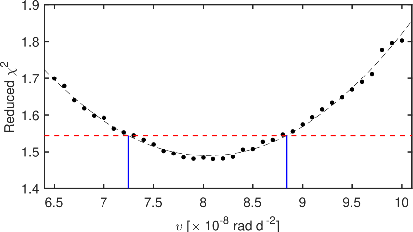
Figure 6: Dependence of the goodness of the fit measured by the reduced $\chi^{2}$ (defined as $\chi^{2}/\nu$, where $\nu$ is the number of degrees of freedom) on the YORP parameter $\upsilon$ for asteroid (10115) 1992 SK. The dashed curve is a quadratic fit of the data points. The dashed red line indicates a $3.7\%$ increase in the $\chi^{2}$, which defines our $1\sigma$ uncertainty interval of $\pm 0.8\times 10^{-8}\,\text{rad}\,\text{d}^{-2}$ given the number of degrees of freedom.

It is interesting to note that the predicted values of the Yarkovsky semimajor axis drift for Geographos are very similar to those of Toro mentioned above (see also Fig. 6 in Vokrouhlický et al., 2005). The larger size of Toro is apparently compensated for by several factors: (i) slightly larger obliquity, (ii) lower perihelion, and (iii) more elongated shape of Geographos, which makes the Yarkovsky effect smaller (e.g., Vokrouhlický, 1998). In spite of a robust Yarkovsky detection for Toro, the current astrometry of Geographos permits for a statistically less significant detection of $(\mathrm{d}a/\mathrm{d}t)=-(1.33\pm 0.42)\times 10^{-4}$ au Myr^-1. The principal reason consists of a wealth of radar data for Toro, suitably distributed over four close encounters with the Earth (including accurate measurements in 2016), and a poorer set of radar measurements for Geographos, over just two close encounters to the Earth in 1983 and 1994. Vokrouhlický et al. (2005) were expecting that the Yarkovsky effect would be firmly detected in the orbit of Geographos by now, but the key element they assumed were accurate astrometric observations in 2008 and/or 2019. Radar observations during the close approach in August 2026 might be an alternative option unless the distance is too large for existing radar systems.

5 Conclusions

It is interesting to compare our determined value of $\upsilon=\mathrm{d}\omega/\mathrm{d}t$ for (10115) 1992 SK with two other exemplary asteroids with good detection of the YORP effect. We ask the readers to first consider the case of (101955) Bennu, for which Hergenrother et al. (2019) obtained $\upsilon=(6.34\pm 0.91)\times 10^{-8}$ rad d^-2, which is slightly smaller than $\upsilon=(8.3\pm 0.6)\times 10^{-8}$ rad d^-2 of (10115) 1992 SK. The two asteroids have approximately the same heliocentric orbits, whose difference has only a very small impact on the YORP effect strength, but the principal difference is due to the following: (i) about twice as small of a size of Bennu as opposed to 1992 SK, (ii) about twice as small of a density of Bennu as opposed to 1992 SK, and (iii) a larger obliquity of Bennu as opposed to 1992 SK (see, e.g., Lauretta et al., 2019). In a simple YORP approach, refraining from the detailed influence of the asteroid shape at various scales, one would thus favor the YORP strength on Bennu by nearly an order of magnitude over that on 1992 SK. Yet, the YORP effect is some $25$% smaller for Bennu. This clearly demonstrates that the shape of Bennu is relatively unfavorable to a strong YORP effect, which is probably due to its high degree of rotational symmetry. On the contrary, the YORP-induced acceleration of (1862) Apollo is $\upsilon=(5.5\pm 1.2)\times 10^{-8}$ rad d^-2 (e.g., Kaasalainen et al., 2007; Ďurech et al., 2008b), which is only a factor of $1.5$ smaller than for 1992 SK. The two asteroids again have similar orbits, both are S-type objects, such that we do not have an a priori reason to suspect a very different bulk density, and even their obliquity is also similar. The main difference then is in about a $50$% larger size of Apollo, such that naively we would expect a factor of $\simeq 2.25$ in their YORP strength (favoring 1992 SK). This is not very different from the observed factor of $\simeq 1.5$, implying that Apollo and 1992 SK are similarly favorable to a non-negligible YORP strength. Indeed, their large-scale resolved shape models are somewhat similar and lack a high degree of symmetry. These examples clearly demonstrate the well known high significance of details of the shape model for the strength of the YORP effect (see Vokrouhlický et al., 2015, and references therein).

A robust result for Geographos, and a slightly weaker, but plausible one, for Toro, illustrate that the possibility to detect the YORP effect is not reserved to the category of very small near-Earth asteroids. Instead, the $2$ to $4$ km class of asteroids is fully accessible for YORP detections if good data are spread over an amenable time interval of a few decades (see also Rozitis & Green, 2013b, for a more formal analysis). In this respect, it might be interesting to carefully review available data for a few kilometer-sized objects and re-analyze their early observations in the 1950s or 1960s. While the astrometric information was used from these frames, the value for photometry had not been tested yet. It is possible that some of these data may reveal interesting constraints on YORP if properly analyzed.

It is also interesting to overview YORP detections that have been achieved so far. Five pre-2015 cases have been summarized in the review chapter by Vokrouhlický et al. (2015). Since then, the YORP detection has been reported for (161989) Cacus by Ďurech et al. (2018b), (101955) Bennu by Hergenrother et al. (2019), (68346) 2001 KZ66 by Zegmott et al. (2021), and Rożek et al. (2019) discussed a plausible YORP determination in the case of (85990) 1999 JV6 (though here its significance is only marginal because of a still short arclength covered by the observations). In this paper, we added a robust YORP detection for (10115) 1992 SK and argue for a weak, but very plausible YORP signal in the case of (1685) Toro (see also Ďurech et al., 2018b). Amazingly enough, all these cases have $\upsilon$ positive, thus implying acceleration of the rotation rate.

The simplest variants of the YORP effect modeling, starting with Rubincam (2000), Vokrouhlický & Čapek (2002), and Čapek & Vokrouhlický (2004), predict about an equal likelihood of a positive and negative value for $\upsilon$ (i.e., rotational acceleration or deceleration by YORP). This result does not appear to change when effects of thermal beaming, due to unresolved small-scale irregularities, and self-irradiation of surface elements are added to the computation, though the overall magnitude of $\upsilon$ may be decreased (e.g., Rozitis & Green, 2012, 2013a). In all these approaches, the thermal modeling is restricted to a one-dimensional conduction below a particular surface facet. Thermal communication of different facets is neglected or limited to mutual irradiation in the model of Rozitis & Green (2013a), but no thermal communication of the surface units is allowed by internal conduction. The idea of the importance of the thermal communication of surface facets via conduction on small-scale surface features was discovered by Golubov & Krugly (2012), and further studied by Golubov et al. (2014), Ševeček et al. (2015), or Ševeček et al. (2016) in more complicated geometries and configurations. The fundamental aspect of mutual conductive contact of different surface units is that it breaks the symmetry in predicted positive and negative $\upsilon$ values for a sample of asteroidal shape models. Instead, the $\upsilon$ value more likely becomes positive than negative, but the degree of this asymmetry depends on a large number of parameters that cannot be easily predicted. So eventually, observations may help to set this asymmetry degree. Given this perspective, we might interpret the YORP detections achieved thus far – not counting the result of Rożek et al. (2019) for (85990) 1999 JV6 – as evidence for a $>10:1$ favor in YORP making the rotation accelerated over decelerated for kilometer-sized near-Earth objects.

While we do not see any a priori selection bias of the asteroids for which YORP has been detected so far, it would be interesting to enlarge the sample of asteroids with a YORP detection for those with larger periods. It is obviously dangerous to draw far-reaching conclusions from a still, very limited sample of only ten objects and even more dangerous to attempt to extrapolate our $\upsilon$-asymmetry guess to a class of few- to ten-kilometer-sized objects in the main belt. Yet, it would be interesting to do so because this population offers some interesting hints about the YORP influence. In particular, Pravec et al. (2008), and more recently Pál et al. (2020), show that there is a significant fraction of these main-belters which rotate slowly. In the situation when planetary encounters are not effective, the YORP effect is suspected to be the primary mechanism to explain this slowly rotating subpopulation. If this is the case, large asymmetry in positive versus negative $\upsilon$ values would imply that the small fraction of asteroids driven to slow rotations must remain in this state for a very long time. But this, in turn, would have an interesting implication on properties of collisional dynamics in the main belt population of objects. However, it is also possible that kilometer-sized, and smaller, near-Earth asteroids have surface properties different from order-of-magnitude larger main belt asteroids. In this case, their $\upsilon$ asymmetry degree may be different. Because the YORP effect is unlikely to be detected among the main-belt asteroids in the foreseeable future, a continuing effort to characterize the YORP properties among a near-Earth population remains a primary objective. In particular, enlarging the sample of cases with both a YORP detection and YORP nondetections (such as 1865 Cerberus discussed in Ďurech et al., 2012) is vital for constraining theoretical concepts of this interesting phenomenon in planetary science.

Appendix A Uncertainty of the YORP parameter

The uncertainties of parameters derived from light curve inversion presented in the main text were determined with bootstrap (Sect. 2). To have an independent estimate, we used the same approach as Vokrouhlický et al. (2011) or Polishook (2014) and computed $\chi^{2}$ for different fixed values of $\upsilon$ (all other parameters were optimized). Then we defined the $1\sigma$ uncertainty interval of $\upsilon$ as such that $\chi^{2}$ increased by a factor of $1+\sqrt{2/\nu}$, where $\nu$ is the number of degrees of freedom. These intervals are larger than those determined by bootstrap.

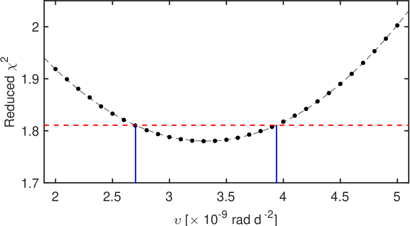
Figure 7: Dependence of the goodness of the fit measured by the reduced $\chi^{2}$ on the YORP parameter $\upsilon$ for asteroid (1685) Toro. The dashed curve is a quadratic fit of the data points. The dashed red line indicates a $1.7\%$ increase in the $\chi^{2}$, which defines our $1\sigma$ uncertainty interval of $\pm 0.6\times 10^{-9}\,\text{rad}\,\text{d}^{-2}$ given the number of degrees of freedom.

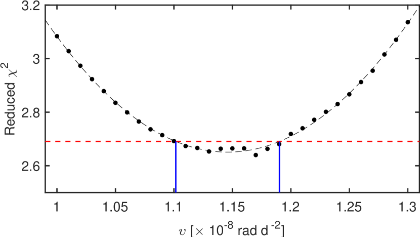
Figure 8: Dependence of the goodness of the fit measured by the reduced $\chi^{2}$ on the YORP parameter $\upsilon$ for asteroid (1620) Geographos. The dashed curve is a quadratic fit of the data points. The dashed red line indicates a $1.5\%$ increase in the $\chi^{2}$, which defines our $1\sigma$ uncertainty interval of $\pm 0.04\times 10^{-8}\,\text{rad}\,\text{d}^{-2}$ given the number of degrees of freedom.

Appendix B Shape models

Appendix C New photometric observations

Table 2: Aspect data for observations of (10115) 1992 SK.

Date	$r$	$\Delta$	$\alpha\phantom{g}$	$\lambda$	$\beta$	Observatory or
	[au]	[au]	[deg]	[deg]	[deg]	Reference
1999 02 08.0	1.195	0.305	41.3	158.3	$50.4$	1
1999 02 09.1	1.189	0.298	41.6	158.1	$50.9$	1
1999 02 09.9	1.185	0.292	41.8	157.9	$51.2$	1
1999 02 15.9	1.153	0.253	44.2	155.6	$53.9$	1
1999 03 11.9	1.028	0.109	68.8	117.2	$63.5$	1
1999 03 13.0	1.022	0.103	71.3	112.4	$63.4$	1
2006 03 06.1	1.017	0.132	75.6	246.0	$40.9$	2
2006 03 07.0	1.012	0.128	77.7	249.7	$39.7$	2
2013 11 03.3	1.591	0.624	12.8	34.0	$19.8$	3
2013 11 05.3	1.595	0.633	13.7	32.9	$20.1$	3
2013 11 06.3	1.597	0.637	14.1	32.3	$20.2$	3
2017 09 26.9	1.193	0.426	53.9	290.7	$-18.2$	KMTNet-SAAO
2017 10 14.1	1.279	0.562	48.2	307.7	$-8.0$	DK
2017 10 14.2	1.280	0.563	48.2	307.8	$-7.9$	DK
2017 10 19.1	1.303	0.609	47.3	311.8	$-5.8$	DK
2017 10 19.2	1.304	0.610	47.2	311.9	$-5.7$	DK
2017 11 12.1	1.409	0.867	44.0	328.2	$1.4$	DK
2020 01 12.3	1.200	0.635	54.9	197.9	$22.0$	DK
2020 10 17.8	1.575	0.644	20.2	53.3	$17.3$	BOAO
2020 10 18.8	1.578	0.642	19.6	52.8	$17.6$	BOAO
2020 10 19.3	1.579	0.642	19.2	52.5	$17.8$	BOAO
2020 10 19.8	1.580	0.641	18.9	52.3	$18.0$	LOAO
2020 10 20.3	1.581	0.640	18.6	52.0	$18.1$	LOAO
2020 10 21.3	1.584	0.639	18.0	51.5	$18.4$	LOAO
2020 11 17.0	1.630	0.695	17.4	36.2	$23.3$	Rozhen
2020 12 04.1	1.647	0.808	25.9	30.0	$22.9$	DK
2020 12 12.8	1.652	0.881	29.4	28.7	$22.2$	Nauchny

(1) Busch et al. (2006); (2) Polishook (2012); (3) Warner (2014)

Table 3: Aspect data for new observations of (1620) Geographos.

(1) Polishook (2009); (2) Skiff et al. (2019); (3) Warner (2016); (4) Warner & Stephens (2019); (5) Warner & Stephens (2020a)

Table 4: Aspect data for new observations of (1685) Toro.

(1) Warner & Stephens (2020b).