Collaborative Radio SLAM for Multiple Robots based on WiFi Fingerprint Similarity

Abstract

Simultaneous Localization and Mapping (SLAM) enables autonomous robots to navigate and execute their tasks through unknown environments. However, performing SLAM in large environments with a single robot is not efficient, and visual or LiDAR-based SLAM requires feature extraction and matching algorithms, which are computationally expensive. In this paper, we present a collaborative SLAM approach with multiple robots using the pervasive WiFi radio signals. A centralized solution is proposed to optimize the trajectory based on the odometry and radio fingerprints collected from multiple robots. To improve the localization accuracy, a novel similarity model is introduced that combines received signal strength (RSS) and detection likelihood of an access point (AP). We perform extensive experiments to demonstrate the effectiveness of the proposed similarity model and collaborative SLAM framework.

I Introduction

The advancement of Simultaneous Localization and Mapping (SLAM) is the key enabler for autonomous navigation, as it deals with self-localization and building a map of unknown environment [1, 2]. Many solutions have been proposed to address this problem in the robotics community during the past decades. With the emergence of low-cost sensors and increasing process power of modern devices, one is able to perform SLAM online and several commercial products (for example Intel RealSense and Google ARCore) are available in the market.

It has been demonstrated that in a single robot application, SLAM is capable of achieving substantial robustness and accuracy [3, 4]. With such achievement, the robotics community research focus has been shifting from high accuracy to high efficiency, resulting usage of multi-robot to perform SLAM. The advantages of leveraging such a technique allow a more robust system to be created by allowing sensing information to be shared among the cluster of robots. It boosts the overall efficiency of a mission by further dividing the SLAM tasks among robots, where a single robot might consume a longer duration to optimize the trajectory. That being said, the multi-robot approach has a few challenges that need to be addressed, such as network reliability, consistency, and information sharing policy.

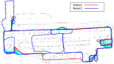
Figure 1: Overview of our collaborative radio SLAM with two robots. We perform SLAM by fusing odometry and radio fingerprints collected from multiple robots. Fingerprint-based constraints between the two robots are shown in cyan.

Collaborative SLAM is one of the common methods leveraging the collaborative nature of multiple robots to perform SLAM. Recent works have been focusing on using different robots for tracking and mapping in unknown environments using unmanned aerial vehicle [5], mobile devices [6, 7], and autonomous robots [8]. Depending on the types of sensors, the complexity of the computation can be high and therefore not suitable for real-time sensing operation. Therefore, selecting a set of useful sensors is essential for developing fast and efficient SLAM.

Nowadays, WiFi networks are abundant in a dense urban area, which are commonly used for data transmission or performing localization in the area where GPS signal is not accessible. It offers low hardware requirement and computational cost due to its ubiquitous in-built sensing capabilities as reviewed in [1]. Hence, analytical models that represent the radio signal distribution are commonly used for trajectory optimization through SLAM [9, 10]. However, they suffered from multipath issues in an uncontrolled environment and hence not suitable in the real-world. That being said, it can be further improved using radio fingerprint [11] resulting in less signal distortion when performing localization. Despite being a less radio distortion approach, a single robot may take a longer time to optimize the pose estimation, which might not be suited for large scale environments. Thus, it motivates us to propose the collaborative radio SLAM in a multi-robot scenario.

In this paper, we present collaborative radio SLAM that performs simultaneous localization and mapping based on the pervasive WiFi signals in a multi-robot scenario, as shown in Figure 1. We investigate the collaborative nature of multiple robots when they actively listen to the surrounding WiFi received signal strength (RSS) measurements from the existing WiFi access points (APs) in an infrastructure. To improve the positioning accuracy, we present a novel similarity measure that considers the received signal strength and the detection likelihood of an AP. Note that this method does not require prior map knowledge nor the access points location, which makes it more suitable for indoor buildings with WiFi network deployed. Using the mutual information concept, the proposed collaborative SLAM solution allows us to improve the pose estimation accuracy by incorporating the measurements from multiple robots. The contributions of this paper are three folded and are listed as follows:

• We propose the collaborative radio SLAM to optimize the trajectory using a multiple-robot scenario based on fingerprint similarity by promoting cooperation among multiple robots.

• A new similarity measure that combines the received signal strength and the detection likelihood of the access point is proposed to improve the localization accuracy.

• We perform extensive experiments to validate the proposed similarity measure as well as our proposed collaborative SLAM solution.

This paper is organized as follows: Section II presents the collaborative mechanism and its theoretical foundation. We then show the experimental results in Section III for different case studies and analyze them. Lastly, we conclude our works in Section IV.

II Collaborative Radio SLAM with Fingerprint Similarity

Figure 1 shows a scenario of two robots perform SLAM in an indoor environment with WiFi. Each robot provides odometry and carries mobile phones to scan the received signal strength of the access point in the environment. The purpose is to perform SLAM by fusing the odometry and radio measurement among all robots without prior knowledge about the infrastructure. While we show only two robots for illustration, the algorithm and discussion are suitable for the general case of multiple robots.

II-A Problem Formulation

Formally, the goal is to estimate the path of robot $k$ up to time $T$: $\mathbf{x}_{k}^{1:T}=\{\mathbf{x}_{k}^{1},...,\mathbf{x}_{k}^{T}\}$, where ${{\mathbf{x}}_{k}^{(t)}}={[x_{k}^{(t)},y_{k}^{(t)},\theta_{k}^{(t)}]}$ denotes the pose of the robot $k$ at time $t$. The radio measurement scanned by robot $k$ at time $t$ is denoted as $\mathbf{f}_{k}^{t}$. Our goal is to estimate the trajectory of all robots given the odometry and radio measurements collected by all robots. We consider a centralized solution, since the data volume of radio measurements is small when compared to the visual images or LiDAR scans.

In general, graph-based SLAM uses the pose of the robot to represent a node. The measurements are decoded as constraints in the graph. The graph-based SLAM aims to find the best configuration of the poses to minimize the error of all constraints through maximum likelihood estimation. In the context of our collaborative SLAM, the constraints consist of three sources: 1) the odometry-based constraints, 2) the individual radio fingerprints-based constraints, and 3) the constraints obtained by comparing the similarity of radio fingerprints collected from different robots. The problem is turned into finding the best poses ${\mathbf{x}^{*}}$ to minimize the following equation:

$$\begin{split}&\operatorname*{arg\,min}_{\mathbf{x}}\sum_{k=1}^{K}\sum_{t=1}^{T}\underbrace{{\mathbf{e}}({\mathbf{x}_{k}^{t-1},\mathbf{x}_{k}^{t},\Delta\mathbf{x}_{k}^{t}})^{T}\Omega_{k}^{t}{\mathbf{e}}({\mathbf{x}_{k}^{t-1},\mathbf{x}_{k}^{t},\Delta\mathbf{x}_{k}^{t}})}_{\text{Odometry-based constraints}}+\\ &\sum_{k=1}^{K}\sum_{(\mathbf{x}_{k}^{i},\mathbf{x}_{k}^{j})\in\mathbf{C}_{k}}\underbrace{{\mathbf{e}}({\mathbf{x}_{k}^{i},\mathbf{x}_{k}^{j},d(\mathbf{f}_{k}^{i},\mathbf{f}_{k}^{j})})^{T}\Omega_{k}^{i,j}{\mathbf{e}}({\mathbf{x}_{k}^{i},\mathbf{x}_{k}^{j},d(\mathbf{f}_{k}^{i},\mathbf{f}_{k}^{j})})}_{\text{Individual radio fingerprint-based constraints}}\\ &+\sum_{(\mathbf{x}_{k}^{i},\mathbf{x}_{l}^{j})\in\mathbf{C}_{k,l}}\underbrace{{\mathbf{e}}({\mathbf{x}_{k}^{i},\mathbf{x}_{l}^{j},d(\mathbf{f}_{k}^{i},\mathbf{f}_{l}^{j})})^{T}\Omega_{k,l}^{i,j}{\mathbf{e}}({\mathbf{x}_{k}^{i},\mathbf{x}_{l}^{j},d(\mathbf{f}_{k}^{i},\mathbf{f}_{l}^{j})})}_{\text{Radio fingerprint-based constraints between robots}}\\ \end{split}$$ (1)

where $K$ is the number of robots moving in the environment. $\mathbf{e}(\cdot)$ denotes the error function, which is computed based on the given poses and the constraints inferred from the observations (i.e., odometry and radio fingerprints). The former is represented as the sequential odometry measurements (a 3$\times 1$ vector including the 2D displacement and the rotation between $\mathbf{x}_{k}^{t-1}$ and $\mathbf{x}_{k}^{t}$). The latter is represented as the fingerprint-based constraint (i.e., a distance measurement $d(\mathbf{f}_{k}^{i},\mathbf{f}_{l}^{j})$ that is determined by the similarity of two radio fingerprints $\mathbf{f}_{k}^{i}$ and $\mathbf{f}_{l}^{j}$, see Section II-C). Similar to our previous work in [7], we train a model to feature the relationship between the distance and the fingerprint similarity. To obtain a better model, we propose a novel similarity measure that additionally considers the detection likelihood of an AP (see Section II-B for details). Constraints are additionally parameterized with a certain degree of uncertainty, which is denoted as the information matrix (i.e., $\Omega_{k}^{t}$, $\Omega_{k}^{i,j}$, and $\Omega_{k,l}^{i,j}$ ) in Equation 1. $\mathbf{C}_{k}$ denotes the set containing the pairs of fingerprint constraints in individual robot $k$ and $\mathbf{C}_{k,l}$ represents the set of fingerprint constraints between robot $k$ and robot $l$.

$$\begin{split}&s_{r}=\prod_{n=1}^{H}\exp(-\frac{(f_{k,n}^{i}-f_{l,n}^{j})^{2}}{2\sigma_{r}^{2}}),\\ \end{split}$$ (2)

where $\sigma_{r}^{2}$ represents the received signal variance, which is set to 36dBm according to [12]. The detection likelihood of extra APs is modeled as:

$$\begin{split}&s_{\tau}=\prod_{n=1}^{M_{k}^{i}}\exp(-\frac{(\tau_{k,n}^{i})^{2}}{2\sigma_{\tau}^{2}})\prod_{n=1}^{M_{l}^{j}}\exp(-\frac{(\tau_{l,n}^{j})^{2}}{2\sigma_{\tau}^{2}}),\\ \end{split}$$ (3)

where $\sigma_{\tau}$ is parameter to control the weights of detection likelihood. The similarity of two fingerprints is modeled as a combination of RSS likelihood of common APs and detection likelihood of extra APs:

$$\begin{split}&s=\mathrm{sim}(\mathbf{f}_{i}^{m},\mathbf{f}_{j}^{n})=s_{\tau}\cdot{\sqrt[H]{s_{r}}}\cdot\frac{H}{H+M_{k}^{i}+M_{l}^{j}}\\ \end{split}$$ (4)

Removing the first term (i.e., $s_{\tau}$) in Equation 4 leads to the Gaussian similarity measure. Our novel similarity measure penalizes the APs with low detection probability and gives better localization results as shown in the experimental results in Section III.

II-B Fingerprint Similarity with RSS and Detection Likelihood

Radio fingerprinting represents location with radio signals from surrounding WiFi APs, which are shown to be robust against location-dependent distortions. The radio fingerprint $\mathbf{f}_{k}^{t}$ recorded at $\mathbf{x}_{k}^{t}$ consists of the average RSS values $\{f_{k,1}^{t},...,f_{k,N}^{t}\}$ and the detection probability $\{\tau_{k,1}^{t},...,\tau_{k,N}^{t}\}$ in a given scanning period, i.e., 5 seconds in our case. Given two fingerprints $\mathbf{f}_{k}^{i}$ and $\mathbf{f}_{l}^{j}$, we use $H$ to represent the number of common APs (i.e., the APs appear in both fingerprints). In addition, let $M_{k}^{i}$ and $M_{l}^{j}$ denote number of extra APs (i.e., the APs appear in only one fingerprint) in $\mathbf{f}_{k}^{i}$ and $\mathbf{f}_{l}^{j}$, respectively. The similarity function $\mathrm{sim}(\mathbf{f}_{k}^{i},\mathbf{f}_{l}^{j})$ yields a positive value between 0 and 1, that considers the signal strength likelihood and the detection likelihood:

II-C Model Training

To optimize Equation 1, we need to know the distance and the variance of two locations based on radio fingerprints. Following our previous work in [7], we train a model to represent the distance and the variance given a similarity by passing over the measurement collected by the robot (i.e., odometry and radio fingerprints), based on the assumption that the odometry is accurate at a short distance (for example 100m).

We first compute similarity for close fingerprint pairs according to Equation 4. These values are annotated with the distance between the two locations obtained by the odometry. As a result, we obtain a set of $W$ training samples: $\{s_{w},d_{w}\}_{w=1}^{W}$, where $s_{w}$ and $d_{w}$ denote the similarity and the distance of a fingerprint pair, which are measured by a similarity measure and the odometry, respectively. We then train a model which characterizes the distance $\hat{d}(s)$ and the variance $\hat{\sigma}^{2}(s)$ given a similarity $s$ by binning:

$$\begin{split}&\hat{d}(s)=\frac{1}{c(\mathbf{b}(s,r))}\sum_{s-\frac{r}{2}\leq s_{w}\leq s+\frac{r}{2}}{d_{w}}\\ &\hat{\sigma}^{2}(s)=\frac{1}{c(\mathbf{b}(s,r))}\sum_{s-\frac{r}{2}\leq s_{w}\leq s+\frac{r}{2}}{(d_{w}-\hat{d}(s))}^{2}\\ \end{split}$$ (5)

where $c(\mathbf{b}(s,r))$ counts the number of samples in interval $r$ given a similarity value $s$. $\hat{d}(s)$ and $\hat{\sigma}^{2}(s)$ represent the expected distance and variance given a similarity $s$.

Data: Odometry of $K$ robots $\{\mathbf{x}_{1}^{1:T},...,\mathbf{x}_{K}^{1:T}\}$ and the associated radio fingerprints $\{\mathbf{f}_{1}^{1:T},...,\mathbf{f}_{K}^{1:T}\}$

Result: Optimized trajectory $\mathbf{x}^{*}$

$\mathcal{C}\leftarrow\varnothing$ // Initial constraint set

// Odometry-based constraints

1 for $k\leftarrow 1$ to $K$ do

2       for $t\leftarrow 1$ to $T$ do

3             $\mathcal{C}\leftarrow\mathcal{C}\cup\langle{\mathbf{e}}({\mathbf{x}_{k}^{t-1},\mathbf{x}_{k}^{t},\Delta\mathbf{x}_{k}^{t}}),\Omega_{k}^{t}\rangle$

4       end for

5      

6 end for

// Fingerprint constraints for individual robot

7 for $k\leftarrow 1$ to $K$ do

8       for $i\leftarrow 1$, $j\leftarrow 1$ to $T$ with $j<i$ do

             // Similarity of $\mathbf{f}_{k}^{i}$ and $\mathbf{f}_{k}^{j}$

9             $s\leftarrow s_{\tau}\cdot{\sqrt[H]{s_{r}}}\cdot\frac{H}{H+M_{k}^{i}+M_{k}^{j}}$ (Equation 4)

10             if $\hat{d}(s)<\nu_{s}$ then

11                  $\mathcal{C}\leftarrow\mathcal{C}\cup\langle{\mathbf{e}}({\mathbf{x}_{k}^{i},\mathbf{x}_{k}^{j},\hat{d}(s)}),\frac{1}{\hat{\sigma}(s)^{2}}\rangle$

12             end if

13            

14       end for

15      

16 end for

// Fingerprint constraints between different robots

17 for $k\leftarrow 1$, $l\leftarrow 1$ to $K$ with $l\neq k$ do

18       for $i\leftarrow 1,j\leftarrow 1$ to $T$ do

             // Similarity of $\mathbf{f}_{k}^{i}$ and $\mathbf{f}_{l}^{j}$

19             $s\leftarrow s_{\tau}\cdot{\sqrt[H]{s_{r}}}\cdot\frac{H}{H+M_{k}^{i}+M_{l}^{j}}$ (Equation 4)

20             if $\hat{d}(s)<\nu_{p}$  then

21                  $\mathcal{C}\leftarrow\mathcal{C}\cup\langle{\mathbf{e}}({\mathbf{x}_{k}^{i},\mathbf{x}_{l}^{j},\hat{d}(s)}),\frac{1}{\hat{\sigma}(s)^{2}}\rangle$

22             end if

23            

24       end for

25      

26 end for

$\rhd$ Pose graph optimization given the constraints $\mathcal{C}$ according to Equation 1

Algorithm 1 Proposed collaborative SLAM

II-D Loop Closure Detection

To optimize the trajectory with graph-based SLAM, we need to find the fingerprint-based constraints (i.e., loop closures) for individual robot and the constraints between different robots. For the individual robot, we first check the distance travelled by the robot between two recorded fingerprints. If it is larger than a pre-defined threshold (100 meters), we compute the similarity based on Equation 4 and obtain the expected distance based on the model in Section II-C. The reason to exclude the close fingerprints for loop closure detection is that the distance measured from odometry in a short period is much precise than the predicted distance obtained from our similarity model in Section II-C. If the expected distance is smaller than a threshold $\nu_{s}$, we add this constraint to the graph for further optimization. Similarly, to detect the fingerprint constraints between different robots, we check the similarity of the fingerprints recorded for different robots. If the expected distance is smaller than a threshold $\nu_{p}$, we add this constraint to the graph. The pose graph is optimized based on g2o (General Graphic Optimization) [13] with an in-build Levenberg-Marquardt solver. An overview of the algorithm is shown in Algorithm 1.

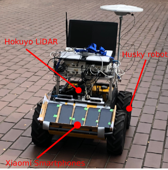
Figure 2: Robot and the sensors used for data collection.

III Experimental Result

In this section, we present the experimental results to validate the proposed approach. In particular, Section III-A describes the experimental setup and Section III-B compares the performance under different similarity measures. Section III-C presents the results of our proposed collaborative radio SLAM.

III-A Experimental Setup

We evaluated the proposed approach at Nanyang Technological University (NTU) Basement 2 carpark B (approx. 5100 m²). The experiments were performed using a Clearpath Husky unmanned ground vehicle, as shown in Figure 2. The robot started at different positions and two test sets (namely, Test I and Test II) were recorded. The robot moved at an average speed of 0.4m/s. Wheel odometry measurements were recorded at a frequency of 10Hz. Five Xiaomi Mi Max3 smartphones were placed on the robot to scan for WiFi access points at a frequency of 0.5Hz. We used a time window of 5 seconds to group the scans from the five phones. We compute average RSS and count detection probability of an AP to create a fingerprint. A Hokuyo 2D LiDAR UST-20LX was mounted on the robot to provide the ground truth through Adaptive Monte Carlo Localization (AMCL) based on a map created by GMapping.

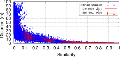
(a) Scatter plot and the model trained using our proposed similarity measure with $\sigma_{r}=6$ and $\sigma_{\tau}=4$

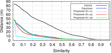
(b) Comparison of the similarity models under different similarity measures

Figure 3: Illustration of the similarity models.

We use a binning size $r=0.05$ to generate the model. The samples used for training and our proposed similarity model is visualized in Figure 3(a). The models generated with different similarity measures are shown in Figure 3(b). As can be seen from this figure, the similarity value computed by our proposed approach is smaller than the Gaussian similarity model, which does not consider the detection likelihood, as our approach additionally penalizes the detection of extra APs. With a large $\sigma_{\tau}$, the proposed model is equivalent to the Gaussian similarity model.

III-B Evaluation of the Proposed Similarity Model

In this series of experiments, we compared the localization accuracy between the proposed similarity model and the existing similarity models, namely Gaussian and cosine. We fix $\sigma_{r}=6$ for this series of experiments. Table I shows the results of single robot SLAM. As can be seen from this table, our proposed similarity model outperforms cosine and Gaussian similarity models in both datasets. With a setting of $\sigma_{\tau}=4$, our proposed model gives the best localization accuracy in both datasets. A too large or too small $\sigma_{\tau}$ leads to decrease in localization accuracy. With our proposed model ($\sigma_{\tau}=4$), we achieve a localization accuracy of 3.261m and 3.364m for Test I and Test II, respectively, which is an improvement of 10.8% and 8.1% when compared to the Gaussian similarity model (i.e., an accuracy of 3.656m and 3.661m for Test I and Test II).

In general, too large or too small $\nu_{s}$ leads to a worse localization result. The best setting of $\nu_{s}$ varies for different datasets. For example, $\nu_{s}=35$ gives the best localization accuracy for Test I, while the best choice for Test II is $\nu_{s}=20$. One reason to explain this is that the odometry exhibits different errors for the two datasets, which requires a different number of constraints (i.e., obtained by different settings of $\nu_{s}$) to compensate for the error.

TABLE I: A comparison of the trajectory estimation accuracy (in meters) under different similarity models with a single robot SLAM.

Experiment	Approach	Setting of parameter $\nu_{s}$
		0	5	10	15	20	25	30	35	40
Test I	Cosine	19.251	4.876	4.723	4.746	4.786	4.691	4.782	4.752	4.563
	Gaussian	19.251	4.573	4.375	4.234	4.062	3.943	3.656	3.849	9.346
	Ours with $\sigma_{\tau}$=1	19.251	4.754	4.337	4.371	4.370	4.370	4.370	4.370	4.543
	Ours with $\sigma_{\tau}$=4	19.251	4.503	4.195	4.167	3.995	3.853	3.618	3.261	3.858
	Ours with $\sigma_{\tau}$=8	19.251	4.552	4.285	4.199	4.085	3.879	3.623	3.665	5.766
Test II	Cosine	10.124	9.137	4.920	4.172	3.838	3.989	6.124	8.788	12.016
	Gaussian	10.124	5.916	4.181	3.661	3.951	7.074	11.97	18.939	24.913
	Ours with $\sigma_{\tau}$=1	10.124	4.816	4.121	4.138	4.138	4.138	4.138	4.339	4.339
	Ours with $\sigma_{\tau}$=4	10.124	5.487	4.040	3.672	3.364	5.789	9.104	11.556	14.133
	Ours with $\sigma_{\tau}$=8	10.124	5.775	4.141	3.729	3.571	6.199	11.1604	18.267	21.301

III-C Evaluation of the Collaborative Radio SLAM

Next, we evaluated the performance of the proposed collaborative radio SLAM. Similar to the previous section, we set $\sigma_{s}=6$. We choose $\sigma_{\tau}=4$ for our proposed similarity measure. The accuracy of optimized trajectory for Test I and Test II are summarized in Table II and Table III, respectively. The results further verify that our proposed similarity measure outperforms cosine and Gaussian similarity measure. In addition, the results show that the proposed solution helps to improve the accuracy of the trajectory estimation by the fusion of measurement from multiple robots. For Test I, with the individual distance threshold $\nu_{s}=10$, our collaborative solution leads to a localization accuracy of 2.774m using $\nu_{p}=30$, which is an improvement of 14.9%, when compared with a single robot SLAM (an accuracy of 3.261m). The same applies to Test II: we obtain a localization accuracy of 2.736m with $\nu_{s}=20$ and $\nu_{p}=10$, which is an improvement of 18.7% when compared to the case without collaborative SLAM (3.364m). Figure 4(a) and Figure 4(b) visualize the trajectory estimated with a single robot and our collaborative SLAM. The best choice of $\nu_{p}$ depends on the settings of $\nu_{s}$ (i.e., the parameter used to infer the individual constraints). In general, we should decrease $\nu_{p}$ with a large $\nu_{s}$ in order to get the best localization accuracy. A too large $\nu_{s}$ will lead to a reduction of the localization accuracy.

TABLE II: Trajectory estimation accuracy of Test I using collaborative SLAM.

$\nu_{s}$	Similarity measures	Settings of parameter $\nu_{p}$
		0	5	10	15	20	25	30	35	40
0	Cosine	19.251	17.607	5.797	5.142	4.245	4.073	3.659	3.975	4.615
	Gaussian	19.251	6.385	4.626	3.590	3.356	3.087	3.974	8.624	18.928
	Ours with $\sigma_{\tau}$=4	19.251	6.718	4.290	3.429	3.201	2.711	2.715	4.931	7.141
5	Cosine	4.876	5.183	4.199	4.196	4.089	3.974	3.773	3.924	4.625
	Gaussian	4.573	3.893	3.729	3.943	3.603	3.166	3.900	8.522	18.745
	Ours with $\sigma_{\tau}$=4	4.503	4.004	3.450	3.426	3.209	2.771	2.787	4.646	6.804
10	Cosine	4.723	4.610	4.381	4.287	4.206	4.063	3.789	3.938	4.638
	Gaussian	4.375	4.013	3.724	3.702	3.445	3.208	3.943	8.346	18.683
	Ours with $\sigma_{\tau}$=4	4.195	3.934	3.462	3.387	3.174	2.847	2.774	4.576	6.716
20	Cosine	4.786	4.648	4.530	4.369	4.231	4.051	3.883	4.081	4.903
	Gaussian	4.062	3.513	3.302	3.254	3.096	3.286	4.600	8.713	18.491
	Ours with $\sigma_{\tau}$=4	3.995	3.557	3.017	3.080	2.844	2.736	2.928	4.821	6.743
30	Cosine	4.782	4.729	4.192	3.939	3.918	3.892	4.046	4.724	5.591
	Gaussian	3.656	3.215	3.424	3.902	4.271	4.867	6.272	9.882	18.818
	Ours with $\sigma_{\tau}$=4	3.618	2.741	2.358	2.689	3.121	3.854	4.267	6.123	7.893
40	Cosine	4.563	4.189	3.979	4.208	4.359	4.687	5.083	5.976	6.598
	Gaussian	9.346	11.662	14.251	14.737	14.900	15.141	15.687	17.100	21.545
	Ours with $\sigma_{\tau}$=4	3.858	4.667	5.345	5.828	6.190	6.763	7.128	8.673	9.971

TABLE III: Trajectory estimation accuracy of Test II using our collaborative SLAM.

$\nu_{s}$	Similarity measures	Settings of parameter $\nu_{p}$
		0	5	10	15	20	25	30	35	40
0	Cosine	10.124	9.224	5.426	5.297	5.07	4.124	4.381	4.608	5.465
	Gaussian	10.124	7.690	4.591	4.182	4.044	4.341	6.262	11.536	22.994
	Ours with $\sigma_{\tau}$=4	10.124	6.009	4.171	4.1322	3.910	4.366	4.914	7.746	10.166
5	Cosine	9.137	8.760	5.492	4.764	3.962	4.032	4.297	4.530	5.395
	Gaussian	5.916	5.384	4.138	3.355	3.289	3.707	5.454	10.757	22.632
	Ours with $\sigma_{\tau}$=4	5.487	4.729	4.407	3.882	3.377	3.682	4.114	6.835	9.541
10	Cosine	4.920	4.727	4.348	3.774	3.576	3.803	4.138	4.374	5.176
	Gaussian	4.181	3.903	3.483	3.185	3.261	3.476	5.025	9.867	21.229
	Ours with $\sigma_{\tau}$=4	4.040	3.959	3.183	3.259	3.256	3.512	3.905	6.289	8.640
20	Cosine	3.838	3.566	3.548	3.519	3.552	4.170	4.490	4.859	5.651
	Gaussian	3.951	3.248	3.259	3.635	3.896	4.481	6.143	10.511	21.661
	Ours with $\sigma_{\tau}$=4	3.364	3.3033	2.736	3.285	3.586	4.105	4.585	7.000	9.267
30	Cosine	6.124	5.566	4.757	4.885	4.985	5.065	5.365	5.861	6.622
	Gaussian	11.97	9.564	8.178	7.944	8.254	8.855	10.246	13.630	22.577
	Ours with $\sigma_{\tau}$=4	9.104	7.547	6.592	6.146	6.411	6.962	7.459	9.464	11.218
40	Cosine	12.016	11.151	9.615	9.207	9.202	9.258	9.360	9.542	10.065
	Gaussian	24.913	22.916	20.832	20.599	20.721	20.927	21.365	22.480	26.288
	Ours with $\sigma_{\tau}$=4	14.133	12.423	10.852	10.481	10.609	11.064	11.355	12.626	13.910

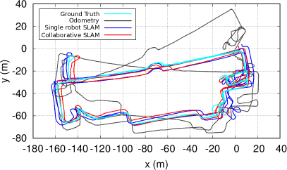
(a) Estimated trajectory for Test I

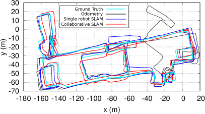
(b) Estimated trajectory for Test II

Figure 4: Estimated trajectory of different test sets under different approaches.

IV Conclusion

We presented a solution for collaborative simultaneous localization and mapping for multiple robots based on radio signals from the pervasive WiFi access points deployed in existing infrastructure. We applied a centralized implementation to fuse the odometry and WiFi radio signals collected from multiple robots. We further proposed a novel similarity measure that incorporates the received signal strength and detection likelihood of an access point. The performance of our approach is validated in a carpark with two sets of experiments. Our results show that our collaborative SLAM improves the trajectory estimation accuracy of a single robot SLAM by integrating the measurements from multiple robots. We achieved an average positioning accuracy of less than 3 meters using our proposed collaborative SLAM and similarity model. In the future, we would like to investigate the possibility to fuse other sensory information, for example other sensor information (i.e., LiDARs), to improve the accuracy of trajectory estimation. Another direction is to develop a fully distributed solution to replace our centralized framework.

References

- [1] A. Yassin, Y. Nasser, M. Awad, A. Al-Dubai, R. Liu, C. Yuen, R. Raulefs, and E. Aboutanios, “Recent advances in indoor localization: A survey on theoretical approaches and applications,” IEEE Communications Surveys Tutorials, vol. 19, no. 2, pp. 1327–1346, Secondquarter 2017.
- [2] B. P. L. Lau, S. H. Marakkalage, Y. Zhou, N. U. Hassan, C. Yuen, M. Zhang, and U.-X. Tan, “A survey of data fusion in smart city applications,” Information Fusion, vol. 52, pp. 357 – 374, 2019.
- [3] R. Mur-Artal, J. M. M. Montiel, and J. D. Tardós, “Orb-slam: A versatile and accurate monocular slam system,” IEEE Transactions on Robotics, vol. 31, no. 5, pp. 1147–1163, Oct 2015.
- [4] R. Liu, Y. He, C. Yuen, B. P. L. Lau, R. Ali, W. Fu, and Z. Cao, “Cost-effective mapping of mobile robot based on the fusion of uwb and short-range 2-d lidar,” IEEE/ASME Transactions on Mechatronics, pp. 1–1, 2021.
- [5] P. Zhang, H. Wang, B. Ding, and S. Shang, “Cloud-based framework for scalable and real-time multi-robot slam,” in 2018 IEEE International Conference on Web Services (ICWS), July 2018, pp. 147–154.
- [6] R. Liu, C. Yuen, T.-N. Do, M. Zhang, Y. L. Guan, and U.-X. Tan, “Cooperative positioning for emergency responders using self imu and peer-to-peer radios measurements,” Information Fusion, vol. 56, pp. 93 – 102, 2020.
- [7] R. Liu, S. H. Marakkalage, M. Padmal, T. Shaganan, C. Yuen, Y. L. Guan, and U. Tan, “Collaborative slam based on wifi fingerprint similarity and motion information,” IEEE Internet of Things Journal, vol. 7, no. 3, pp. 1826–1840, March 2020.
- [8] Z. Cao, R. Liu, C. Yuen, A. Athukorala, B. K. K. Ng, M. Mathanraj, and U. Tan, “Relative localization of mobile robots with multiple ultra-wideband ranging measurements,” in 2021 IEEE/RSJ International Conference on Intelligent Robots and Systems (IROS 2021), Prague, Czech Republic, September 27–October 1 2021.
- [9] B. Ferris, D. Fox, and N. D. Lawrence, “Wifi-slam using gaussian process latent variable models.” in IJCAI, vol. 7, no. 1, 2007, pp. 2480–2485.
- [10] J. Huang, D. Millman, M. Quigley, D. Stavens, S. Thrun, and A. Aggarwal, “Efficient, generalized indoor wifi graphslam,” in 2011 IEEE International Conference on Robotics and Automation, May 2011, pp. 1038–1043.
- [11] M. Zhou, Y. Tang, Z. Tian, L. Xie, and W. Nie, “Robust neighborhood graphing for semi-supervised indoor localization with light-loaded location fingerprinting,” IEEE Internet of Things Journal, vol. 5, no. 5, pp. 3378–3387, 2018.
- [12] R. Berkvens, A. Jacobson, M. Milford, H. Peremans, and M. Weyn, “Biologically inspired slam using wi-fi,” in 2014 IEEE/RSJ International Conference on Intelligent Robots and Systems, September 14-18 2014, pp. 1804–1811.
- [13] G. Grisetti, R. Kümmerle, C. Stachniss, and W. Burgard, “A tutorial on graph-based slam,” IEEE Intelligent Transportation Systems Magazine, vol. 2, no. 4, pp. 31–43, winter 2010.