New allocation rule of directed hypergraphs

Abstract.

The Shapley value, one of the well-known allocation rules in game theory, does not take into account information about the structure of the graph, so by using the Shapley value for each hyperedge, we introduce a new allocation rule by considering their first-order combination. We proved that some of the properties that hold for Shapley and Myerson values also hold for our allocation rule. In addition, we found the relationship between our allocation rule and the Forman curvature, which plays an important role in discrete geometry.

1. Introduction

1.1. Background

Game theory can be classified into types—cooperative and noncooperative. In cooperative game theory, all players cooperate with each other to increase their utility, thereby forming a coalition and generating worth. The cooperative game theory is employed in several analyses, including those of markets in economics, bill votes by political parties, and cost sharing. Recently, it has also found application in market design by way of auction and matching theories. The primary focus in the application of these theories concerns the sharing or distribution of the worth gained from a cooperation. To this end, we usually consider a transferable utility or TU game. In 1953, Shapley introduced the Shapley value [Sh] based on the results of one of the most famous investigations concerning this topic. Although it corresponds to a method of fairly distributing the worth gained from a cooperation, it is assumed there exist no restrictions on the cooperation possibilities of the players. To solve this problem, in 1977, Myerson introduced a graph-restricted game by modifying the original game and defined the corresponding Shapley value, namely the Myerson value [My]. Subsequently, several studies have been conducted concerning the Myerson value. An interesting topic, which has hitherto been seldom investigated in available literature, concerns the type of cooperative network. Initially, Myerson considered an undirected graph as a cooperative network. Therefore, Li–Shan considered the Myerson value for a directed graph [LS2], and Nouweland–Borm–Tijs considered the Myerson value for a hypergraph [VDN]. Another topic of research concerns the characterization of the Myerson value. In 2001, Algaba–Bilbao–Borm–Lopez characterized the Myerson value for union stable structures [ABBL]. In 2004, Gomez—Gonzalez–Manuel—Owen—Pozo–Tejada calculated the Myerson value of splitting graphs for pure overhead games [GGMO]. In 2012, Kim–Hee introduced various concepts of betweenness and centrality. Moreover, they deduced the relationship between them and the Myerson value [Kim]. In 2016, Beal—Casajus–Huettner studied the efficient egalitarian Myerson value [BA]. In 2021, Wang–Shan proved the decomposition property for the weighted Myerson value [WE].

The Ricci curvature is one of the most important concepts in Riemannian geometry. There are some definitions of generalized Ricci curvature, one of which is Forman Ricci curvature. In the case of undirected graphs, Forman curvature is defined by

$$F((x,y))=4-d(x)-d(y),$$

where $(x,y)$ is an edge, and $d(x)$ is a degree of $x$ (the number of edges connecting $x$). On the other hand, in the case of directed graphs,

$$F((x,y))=2-d^{\mathrm{in}}(x)-d^{\mathrm{out}}(y).$$

Recently, Leal-Restrepo-Stadler-Jost [LGJ] defined the Forman curvature on directed hypergraphs. By the definition of Forman curvature, the larger the degree of the vertices of the edge, the more negative Forman curvature is. For this reason, Forman curvature has often been used as a tool to determine the importance of edges.

1.2. Our motivation

In fact, manufacturers like Apple buy various components from other companies to produce their final products. To make each component to be delivered to the manufacturer, a company needs to hire researchers or borrow money from a bank. The companies supplying the components also supply other manufacturers. Such firms are, however, neither exclusive nor comprehensive. Some firms may supply in several makers, while others may supply in no maker. Many maker have overlapping firms. The firms overlapped in more than one maker may play the role of mediating information between maker. Thus, through the mediator, a firm can get indirect benefits from the maker to which he does not belong. Joining in a maker does not only yield (direct and indirect) benefits but also incurs some costs. For example, a firm may be constrained in its sales to deliver parts to a manufacturer.

It is important for manufacturers to consider how to efficiently distribute the profits earned from the sale of their products to the firms that supplied the components. In addition, he enjoys indirect benefits from firms in different maker who are indirectly connected through the firm of his maker.

In order to consider how to efficiently distribute profits to each company in such a situation, it is very effective to use hypergraphs, which are a generalization of graphs, instead of the conventional analysis using graphs. Specifically, the vertices of the hypergraph are defined as companies that manufacture parts, and the edges of the hypergraph are defined as a collection of companies that manufacture the parts necessary to produce the final product. However, when defining the hypergraph in this way, there is a problem that for each company, the parts that need to be purchased from other companies are divided into those that cannot be supplied by the company itself and those that are cheaper than those supplied by the company itself. Thus, it is best to consider a mathematical model using a directed hypergraph that can partition the firms that supplied the parts. For this reason, in this paper, we consider a directed hypergraph, a natural generalization of an undirected graph, a directed graph, and undirected hypergraph, as a cooperative network. In graph theory, many properties that hold for graphs also hold for hypergraphs, so the study of hypergraphs has a wide range of applications. However, studies involving directed hypergraphs are challenging compared to those involving graphs since the number of vertices containing an edge on a directed hypergraph usually exceeds 2, and each edge is oriented.

In this paper, the allocation rule we use is newly defined based on Shapley values to better reflect the structure of the graph, and called the individual Shapley value. We proved that some of the properties that hold for Shapley and Myerson values also hold for our allocation rule. In addition, we found the relationship between our allocation rule and the Forman curvature, which plays an important role in discrete geometry.

The remainder of this paper is organized as follows. Section 2 presents the basic notations and properties of the Shapley value and the Myerson value. Section 3 presents the definition of the individual Shapley value, and properties of the individual Shapley value. Section 4 presents relationship with Forman curvature. We give concrete characteristic functions, and prove some properties. Section 5 describes the calculation of the individual Shapley value on a specific directed hypergraph. Finally, Section 6 lists the major conclusions drawn from this study and identifies the scope for future research.

2. Preliminaries

2.1. Notation about graph theory

Let $H=(N,E)$ be a directed hypergraph, wherein $N$ denotes a set of players $N=\left\{1,\cdots,n\right\}$ and $E$ is a subset of $2^{N}$. Every hyperedge $e\in E$ represents a directional relation between two non-empty subsets $A_{e}$ and $B_{e}$ of $N$ (see Figure 1). Accordingly, $A_{e}$ and $B_{e}$ represent the tail and head sets of $e$, respectively. Sometimes a player $v_{i}\in V$ is simply written as $i$.

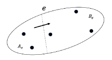
Figure 1. Directed hyperedge

Definition 2.1.

For any two players $s$ and $t$, a directed path from $s$ to $t$ represents a sequence of players and hyperedges $(s=v_{0},e_{0},v_{1},e_{1},\cdots,e_{l-1},v_{l}=t)$, where

$$s\in A_{e_{0}},\ t\in B_{e_{l-1}},\ \mathrm{and}\ v_{i}\in A_{e_{i}}\cap B_{e_{i+1}}$$

for any $i\in\left\{1,\cdots,l-1\right\}$.

If there exist directed paths from $s$ to $t$ or $t$ to $s$, then $s$ and $t$ is called connected. Moreover, if any pair of players in $N$ is connected, then $H=(N,E)$ is called connected.

Definition 2.2.

An induced subgraph $H^{\prime}$ of $H=(N,E)$ represents a pair of $(N_{H^{\prime}},E_{H^{\prime}})$ that satisfy $N_{H^{\prime}}\subseteq N$ and

$$E_{H^{\prime}}=\left\{e\mid e\in E,\ e\subseteq N_{H^{\prime}}\right\}.$$

A maximal connected induced subgraph is called the component of $H$, and $N/E$ denotes the set of all components in $H$. Note that the union of all components in $H$ equals $N$.

2.2. Notation about game theory

The TU game represents a pair $(N,v)$, where $N$ denotes a set of players and $v:2^{N}\to\mathbb{R}$ is a characteristic function with $v(\emptyset)=0$. Each $S\in 2^{N}$ is referred to as a coalition, and $v(S)$ represents the worth of $S$. The set of all TU games is denoted by $TU(N)$. A directed hypergraph game on $N$ represents a triplet $(N,v,E)$ such that $(N,v)$ is a TU game and $(N,E)$ is a directed hypergraph. The set of all directed hypergraph games are denoted by $DHG(N)$.

Definition 2.3.

Given $(N,v)\in TU(N)$,

1. $v$ is called super additive if for any $S,T\in 2^{N}$ with $S\cap T=\emptyset$, $v(S\cup T)\geq v(S)+v(T)$.

2. $v$ is called sub additive if for any $S,T\in 2^{N}$ with $S\cap T=\emptyset$, $v(S\cup T)\leq v(S)+v(T)$.

Now, define Shapley value, one of the famous allocation rules.

$$Sh_{i}(N,v)=\sum_{S\subseteq N\setminus\left\{i\right\}}\cfrac{s!(n-s-1)!}{n!}(v(S\cup\left\{i\right\})-v(S)).$$

We review one of the important theorems about the Shapley value.

Theorem 2.4 ([Sh]).

The Shapley value can be uniquely determined as efficient, additive, symmetric, and conforming to the null-player property subject to the following conditions.

1. An allocation rule $f$ on $TU(N)$ is efficient if for any $(N,v)\in TU(N)$,

   $$\sum_{i\in N}f_{i}(N,v)=v(N).$$

2. An allocation rule $f$ on $TU(N)$ is additive if for all $(N,v),(N,w)\in TU(N)$,

   $$f(N,v+w)=f(N,v)+f(N,w).$$

3. An allocation rule $f$ on $TU(N)$ is symmetric if for any $(N,v)\in TU(N)$,

   $$f_{i}(N,v)=f_{j}(N,v)$$

   for any two players $i,j\in N$ with $v(S\cup\left\{i\right\})=v(S\cup\left\{j\right\})$ for all $S\subseteq N\setminus\left\{i,j\right\}$.

4. An allocation rule $f$ on $TU(N)$ satisfies the null-player property if for any $(N,v)\in TU(N)$,

   $$f_{i}(N,v)=0$$

   for any $i\in N$ with $v(S)=v(S\cup\left\{i\right\})$ for all $S\subseteq N$.

As can be seen from the theorem, the Shapley value is an excellent allocation rule that satisfies the property, but does not take graph structure into account. One solution to this problem is an allocation rule called Myerson value. The Myerson value $\mu(N,v,E)$ can be expressed as

$$\mu_{i}(N,v,E)=Sh_{i}(N,v^{E})=\sum_{S\subseteq N\setminus\left\{i\right\}}\cfrac{s!(n-s-1)!}{n!}(v^{E}(S\cup\left\{i\right\})-v^{E}(S)),$$

where $v^{E}(S)=\sum_{T\in S/E_{S}}v(T)$ for any coalition $S$. We review one of the important theorems about the Myerson value.

Theorem 2.5 ([My], [LS2]).

For any $(N,v,E)\in DHG(N)$, the Myerson value represents a unique allocation rule that satisfies the conditions of component efficiency and fairness, where

1. an allocation rule $f$ on $DHG(N)$ is component efficient if for any $(N,v,E)\in DHG(N)$,

   $$\sum_{i\in T}f_{i}(N,v,E)=v(T)$$

   for any component $T\in N/E$, and

2. an allocation rule $f$ on $DHG(N)$ is fair if for any $(N,v,E)\in DHG(N)$,

   $$f_{i}(N,v,E)-f_{i}(N,v,E\setminus e)=f_{j}(N,v,E)-f_{j}(N,v,E\setminus e)$$

   for any $e\in E$ with $i\in A_{e}$ and $j\in B_{e}$.

Myerson value is an allocation rule that reflects the connected components of the graph, but we want to introduce an allocation rule that uses the graph structure more precisely.

3. Individual Shapley value

3.1. Definition

We would like to apply this research to a directed hypergraph where the vertex set is a company that manufactures parts and the edge set is a company that manufactures the final product. In this case, it is natural to assume that the value of a component is different for each company. Therefore, we define the following characteristic function.

Definition 3.1.

Let $(N,E)$ be a directed hypergraph.

1. For a hyperedge $e\in E$, a map $w_{e}:2^{e}\to\mathbb{R}$ is an edge-characteristic function with $w_{e}(\emptyset)=0$.

2. For edge-characteristic functions $\left\{w_{e}\right\}_{e\in E}$, a whole characteristic function, denoted by $v^{w}$, is defined by a map $v^{w}:2^{N}\to\mathbb{R}$ satisfying for any coalition $S\in 2^{N}$,

   $$v^{w}(S)=\sum_{e\in E}w_{e}(e\cap S).$$

The following relationship exists between an edge characteristic function and a whole characteristic function.

Lemma 3.2.

Let $v^{w}$ be a whole characteristic function. For any hyperedge $e$, if $w_{e}$ is a super additive, then $v^{w}$ is also a super additive. The same argument holds true for sub additive.

Proof.

Since the sub additivity case can be proved in the same way, we prove only the super additivity case. For any $S,T\in 2^{N}$ with $S\cap T=\emptyset$, we have

$$v^{w}(S\cup T) = \sum_{e\in E}w_{e}(e\cap(S\cup T))$$

$$= \sum_{e\in E}w_{e}((e\cap S)\cup(e\cap T))$$

$$\geq \sum_{e\in E}w_{e}(e\cap S)+\sum_{e\in E}w_{e}(e\cap T)=v^{w}(S)+v^{w}(T).$$

∎

We define a new allocation rule by using a whole characteristic function.

Definition 3.3.

The individual Shapley value is defined by

$$ISh_{i}(N,v^{w},E)=\sum_{e\in E_{i}}Sh_{i}(e,w_{e}),$$

where $E_{i}:=\left\{e\in E\mid i\in E\right\}$. By the concept of the Shapley value, we define $Sh_{i}(e,w_{e})=0$ if $i\notin e$.

3.2. Comparison of the previous properties

We check how the properties of Shapley value and Myerson value, as described in Theorem 2.4 and Theorem 2.5, are changed in individual Shapley value.

Proposition 3.4.

The individual Shapley value is satisfies efficiency, additivity and component efficiency.

Proof.

To show the efficiency, we calculate as follows;

$$\sum_{i\in N}ISh_{i}(N,v^{w},E) = \sum_{i\in N}\sum_{e\in E_{i}}Sh_{i}(e,w_{e})$$

$$= \sum_{e\in E}\sum_{i\in e}Sh_{i}(e,w_{e})=\sum_{e\in E}w_{e}(e)=v^{w}(N).$$

Next, we show the additivity. For two distinct edge-characteristic functions $w,w^{\prime}$, we calculate as follows;

$$ISh_{i}(N,v^{w+w^{\prime}},E) = \sum_{e\in E_{i}}Sh_{i}(e,w_{e}+w^{\prime}_{e})$$

$$= \sum_{e\in E_{i}}Sh_{i}(e,w_{e})+\sum_{e\in E_{i}}Sh_{i}(e,w^{\prime}_{e})=ISh_{i}(N,v^{w},E)+ISh_{i}(N,v^{w^{\prime}},E).$$

Finally, we show the component efficiency. For simplicity, let $H/E=\left\{T_{1},T_{2}\right\}$ be the set of all components in $H$. For any $i\in T_{1}$, we assume that there exists a player $j$ such that $j\in T_{2}\cap\bigcup_{e\in E_{i}}e$. Then, there exists a path between $i$ and $j$ since $j\in\bigcup_{e\in E_{i}}e$. However, this contradicts $j\in T_{2}$. Thus we have $E_{i}\subseteq T_{1}$ for any $i\in T_{1}$, so we calculate as follows.

$$\sum_{i\in T_{1}}ISh_{i}(N,v^{w},E) = \sum_{i\in T_{1}}\sum_{e\in E_{i}}Sh_{i}(e,w_{e})$$

$$= \sum_{e\in E_{T_{1}}}\sum_{i\in e}Sh_{i}(e,w_{e})=\sum_{e\in E_{T_{1}}}w_{e}(e)=v^{w}(T_{1}).$$

The proof is completed. ∎

Remark 3.5.

If all properties of Theorem 2.4 hold, then by uniqueness, $ISh=Sh$. However, the individual Shapley value does not satisfy symmetry and null-player property. On the other hand, if all properties of Theorem 2.5 hold, then by uniqueness, $ISh=\mu$. However, the individual Shapley value does not satisfy fairness.

3.2.1. Symmetry and fairness

In this section, we will mention the symmetry and fairness of the individual Shapley value. For any player $i$ and $j$, symmetry does not hold because the hyperedge containing $i$ and the hyperedge containing $j$ are not necessarily coincident. Therefore, it is necessary to identify an alternative property to symmetry.

Lemma 3.6.

Let $(N,v,E)$ be a directed hypergraph game. Suppose that there exist two players $i,j\in N$ with $E_{i}=E_{j}$ such that for any $e\in E_{i}(=E_{j})$, we have

$$w_{e}(S\cup\left\{i\right\})=w_{e}(S\cup\left\{j\right\}),$$

for any subset $S\subseteq e\setminus\left\{i,j\right\}$. Then we have

$$ISh_{i}(N,v^{w})=ISh_{j}(N,v^{w}).$$

Proof.

By the assumption, for any $e\in E_{i}(=E_{j})$, we have

$$Sh_{i}(e,w_{e})=Sh_{j}(e,w_{e}).$$

Thus, we have

$$ISh_{i}(N,v^{w}) = \sum_{e\in E_{i}}Sh_{i}(e,w_{e})$$

$$= \sum_{e\in E_{j}}Sh_{j}(e,w_{e})=ISh_{j}(N,v).$$

Then the proof is completed. ∎

Remark 3.7.

In the case of a graph satisfying the above assumptions, the graph is only $G=(\left\{i,j\right\},\left\{\left\{i,j\right\}\right\})$ (see bottom of Figure 2). However, there exist many directed hypergraphs satisfying the above assumption (see upper of Figure 2).

Figure 2. Upper: Hypergraph satisfying the assumption. Bottom: Simple graph satisfying the assumption.

By the definition of the individual Shapley value, for any edge $e_{0}\in E$ and any $i\in e$, we have

$$ISh_{i}(N,v^{w},E)-ISh_{i}(N,v^{w},E\setminus e_{0})=Sh_{i}(e_{0},w_{e_{0}}).$$ ( 3.1)

Combining the equation (3.1) and Lemma 3.6, we obtain the following corollary.

Corollary 3.8.

Let $e$ be a hyperedge. For any two players $i,j\in N$ with $w_{e}(S\cup\left\{i\right\})=w_{e}(S\cup\left\{j\right\})$ for all $S\subseteq e\setminus\left\{i,j\right\}$, we have

$$ISh_{i}(N,v^{w},E)-ISh_{i}(N,v^{w},E\setminus e)=ISh_{j}(N,v^{w},E)-ISh_{j}(N,v^{w},E\setminus e).$$

3.2.2. Null-player property

In this section, we will mention the null-player property of the individual Shapley value. To show the null-player property, we have

$$ISh_{i}(N,v^{w},E) = \sum_{e\in E_{i}}Sh_{i}(e,w_{e})$$

$$= \sum_{e\in E_{i}}\sum_{S\subseteq e\setminus\left\{i\right\}}\cfrac{s!(|e|-s-1)!}{|e|!}(w_{e}(S\cup\left\{i\right\})-w_{e}(S)).$$

Thus, if for any $e\in E_{i}$ and any $S\subseteq e\setminus\left\{i\right\}$, it holds that

$$w_{e}(S\cup\left\{i\right\})=w_{e}(S),$$ ( 3.2)

then we have $ISh_{i}(N,v^{w},E)=0$. However, if we apply the assumption of the null-player property to the individual Shapley value, then we represent that for any $i\in N$ and any $S\subseteq N$,

$$v^{w}(S)=v^{w}(S\cup\left\{i\right\}),$$

which implies

$$v^{w}(S\cup\left\{i\right\})-v^{w}(S) = \sum_{e\in E}(w_{e}(e\cap(S\cup\left\{i\right\}))-w_{e}(e\cap S))$$

$$= \sum_{e\in E_{i}}(w_{e}(e\cap(S\cup\left\{i\right\}))-w_{e}(e\cap S))=0.$$

From this assumption, we do not obtain the equation (3.2). In fact, we consider the directed hypergraph $H=(N,\left\{e_{1},e_{2}\right\})$, where $A_{e_{1}}=B_{e_{2}}$ and $A_{e_{2}}=B_{e_{1}}$ (see Figure 3). If we give the following edge-characteristic functions,

$$w_{e_{1}}(S)=|S|,\ w_{e_{2}}(S)=|e_{2}|-|S|,$$

for any $S\subseteq 2^{N}$, then we have

$$v^{w}(S\cup\left\{i\right\})-v^{w}(S)=(w_{e_{1}}(S\cup\left\{i\right\})-w_{e_{1}}(S))+(w_{e_{2}}(S\cup\left\{i\right\})-w_{e_{2}}(S))=0.$$

However, it does not holds the equation (3.2).

Figure 3. Counterexample of null-player property

4. Relationship with Forman curvature

In this section we show the relationship with Forman curvature. First, we define a Forman curvature.

Definition 4.1 ([LGJ]).

For a hyperedge $e\in E$,

1. the Forman curvature for the in flow at $A_{e}$ is defined by

   $$F({}_{\rightarrow}e)=|A_{e}|-\sum_{i\in A_{e}}d^{\mathrm{in}}(i).$$

2. the Forman curvature for the out flow at $B_{e}$ is defined by

   $$F(e_{\rightarrow})=|B_{e}|-\sum_{j\in B_{e}}d^{\mathrm{out}}(i).$$

3. the Forman curvature for the total flow through $e$ is defined by

   $$F({}_{\rightarrow}e_{\rightarrow}) = F({}_{\rightarrow}e)+F(e_{\rightarrow})$$

   $$= |A_{e}|+|B_{e}|-\sum_{i\in A_{e}}d^{\mathrm{in}}(i)-\sum_{j\in B_{e}}d^{\mathrm{out}}(i).$$

As can be seen from the definition, the greater the number of edges passing through edge $e$, the more negative the Forman curvature is. The edges with the most negative values play an important role in graph analysis, but the importance of the vertices on those edges cannot be measured. We would like to rank the vertices using the individual Shapley value, so we consider the following edge-characteristic functions. For a hyperedge $e\in E$,

$$w_{e}(S)=-(|S\cap A_{e}|-\sum_{i\in S\cap A_{e}}d^{\mathrm{in}}(i)),$$

$$w^{\prime}_{e}(S)=-(|S\cap B_{e}|-\sum_{i\in S\cap B_{e}}d^{\mathrm{out}}(i))$$

for any $S\subseteq 2^{e}$. Then we obtain

$$w_{e}(e)=-F({}_{\rightarrow}e),\ w^{\prime}_{e}(e)=-F(e_{\rightarrow}).$$

Moreover, for any $S,T\subseteq 2^{e}$ with $S\cap T=\emptyset$, we have

$$w_{e}(S\cup T)=w_{e}(S)+w_{e}(T),\ w^{\prime}_{e}(S\cup T)=w^{\prime}_{e}(S)+w^{\prime}_{e}(T).$$ ( 4.1)

The relationship between Forman curvature and individual Shapley value is as follows.

Lemma 4.2.

For any edge $e\in E$, we have

$$\sum_{i\in e}(ISh_{i}(N,v^{w},E)-ISh_{i}(N,v^{w},E\setminus e))=-F({}_{\rightarrow}e),$$

$$\sum_{i\in e}(ISh_{i}(N,v^{w^{\prime}},E)-ISh_{i}(N,v^{w^{\prime}},E\setminus e))=-F(e_{\rightarrow}).$$

Proof.

Since similar arguments can be made, only the first equation is proved. By the equation (3.1), for any edge $e\in E$, we have

$$ISh_{i}(N,v^{w},E)-ISh_{i}(N,v^{w},E\setminus e)=Sh_{i}(e_{0},w_{e}).$$

Thus, by the efficiency of the Shapley value, we obtain

$$\sum_{i\in e}(ISh_{i}(N,v^{w},E)-ISh_{i}(N,v^{w},E\setminus e))=\sum_{i\in E}Sh_{i}(e,w_{e})=w_{e}(e)=-F({}_{\rightarrow}e).$$

∎

More specifically, the individual Shapley value can be expressed as follows.

Theorem 4.3.

For any player $i\in N$, we have

$$ISh_{i}(N,v^{w}+v^{w^{\prime}},E)=2d^{\mathrm{in}}(i)d^{\mathrm{out}}(i)-d^{\mathrm{in}}(i)-d^{\mathrm{out}}(i).$$

Proof.

For any hyperedge $e\in E$, by the definition of $w_{e}$, we have

$$w_{e}(\left\{i\right\}) = -(|\left\{i\right\}\cap A_{e}|-\sum_{j\in\left\{i\right\}\cap A_{e}}d^{\mathrm{in}}(j))$$

$$= \begin{cases}-(1-d^{\mathrm{in}}(i)),&\textit{if}\ i\in A_{e},\\ 0,&\textit{if}\ i\in B_{e}.\end{cases}$$

By using this and the equation (4.1), we calculate as follows.

$$ISh_{i}(N,v^{w},E) = \sum_{e\in E_{i}}\sum_{S\subseteq e\setminus\left\{i\right\}}\cfrac{s!(|e|-s-1)!}{|e|!}(w_{e}(S\cup\left\{i\right\})-w_{e}(S))$$

$$= \sum_{e\in E_{i}}\sum_{S\subseteq e\setminus\left\{i\right\}}\cfrac{s!(|e|-s-1)!}{|e|!}w_{e}(\left\{i\right\})$$

$$= \sum_{e\in E_{i}}w_{e}(\left\{i\right\})=-d^{\mathrm{out}}(i)(1-d^{\mathrm{in}}(i)).$$

Similarly, we obtain $ISh_{i}(N,v^{w^{\prime}},E)=-d^{\mathrm{in}}(i)(1-d^{\mathrm{out}}(i))$. By Proposition 3.4, we have

$$ISh_{i}(N,v^{w}+v^{w^{\prime}},E) = ISh_{i}(N,v^{w},E)+ISh_{i}(N,v^{w^{\prime}},E)$$

$$= -d^{\mathrm{out}}(i)(1-d^{\mathrm{in}}(i))-d^{\mathrm{in}}(i)(1-d^{\mathrm{out}}(i))$$

$$= 2d^{\mathrm{in}}(i)d^{\mathrm{out}}(i)-d^{\mathrm{in}}(i)-d^{\mathrm{out}}(i).$$

The proof is completed. ∎

5. Example

In this section, we calculated the individual Shapley value for each player depicted in Figure 4. Considering $H=(N,E)$ denotes the hypergraph in Figure 4, it can be stated that

$$N = \left\{1,2,3,4,5,6,7\right\},$$

$$E = \left\{e_{1}=\left\{1,2\right\},e_{2}=\left\{1,2\right\},e_{3}=\left\{2,3,4\right\},e_{4}=\left\{1,3,4,5\right\},e_{5}=\left\{4,6,7\right\},e_{6}=\left\{2,6,7\right\}\right\},$$

where

$$A_{e_{1}}=\left\{1\right\},\ B_{e_{1}}=\left\{2\right\},$$

$$A_{e_{2}}=\left\{2\right\},\ B_{e_{2}}=\left\{1\right\},$$

$$A_{e_{3}}=\left\{2,3\right\},\ B_{e_{3}}=\left\{4\right\},$$

$$A_{e_{4}}=\left\{3,4,5\right\},\ B_{e_{4}}=\left\{1\right\},$$

$$A_{e_{5}}=\left\{4\right\},\ B_{e_{5}}=\left\{6,7\right\},$$

$$A_{e_{6}}=\left\{6,7\right\},\ B_{e_{6}}=\left\{2\right\}.$$

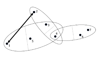
Figure 4. Directed hypergraph

To interpret this directed hypergraph as a mathematical model of the real world, we consider the smartphone industry. The vertices $N$ of the hypergraph correspond to five component manufacturing companies, e.g., Qualcomm, Sharp, and Samsung. The edges $E$ of the hypergraph correspond to four smartphone manufacturing companies. To explain the orientation of the edges, we focus on $e_{1}$. Component firm $1$ manufactures parts that $e_{1}$ cannot supply itself, and component firm $2$ manufactures parts cheaper than $e_{1}$ can supply itself. On the other hand, looking at $e_{3}$, component firms $2$ and $3$ produce parts that $e_{3}$ cannot supply itself, and component firm $4$ produces parts cheaper than $e_{3}$ can supply itself. The same holds for $e_{2}$, $e_{4}$, $e_{5}$ and $e_{6}$.

Considering the original characteristic functions as described earlier , we have

$$w_{e_{1}}(e_{1})=1,\ w_{e_{2}}(e_{2})=1,\ w_{e_{3}}(e_{3})=0,\ w_{e_{4}}(e_{4})=-2,\ w_{e_{5}}(e_{5})=0,\ w_{e_{6}}(e_{6})=0,$$

$$w^{\prime}_{e_{1}}(e_{1})=1,\ w^{\prime}_{e_{2}}(e_{2})=0,\ w^{\prime}_{e_{3}}(e_{3})=1,\ w^{\prime}_{e_{4}}(e_{4})=0,\ w^{\prime}_{e_{5}}(e_{5})=0,\ w^{\prime}_{e_{6}}(e_{6})=1,$$

which implies

$$F({}_{\rightarrow}e_{1}{}_{\rightarrow})=-2,\ F({}_{\rightarrow}e_{2}{}_{\rightarrow})=-1,\ F({}_{\rightarrow}e_{3}{}_{\rightarrow})=-1,$$

$$F({}_{\rightarrow}e_{4}{}_{\rightarrow})=2,\ F({}_{\rightarrow}e_{5}{}_{\rightarrow})=0,\ F({}_{\rightarrow}e_{6}{}_{\rightarrow})=-1.$$

Thus, we calculate the individual Shapley value as follows.

$$ISh(N,v^{D},E)=\left(1,4,-2,1,-1,0,0\right).$$

From these results, we can say that the most important edge is $e_{1}$ and the most important vertex is 2.

6. Conclusions

In this paper, we define a new allocation rule using the Shapley value of each edge to reflect the graph structure better than Shapley value or Myerson value. This allocation rule is called individual Shapley value, and we proved that some of the properties of Shapley value and Myerson value also hold for individual Shapley value. Furthermore, we proved the relationship with Forman curvature, which plays an important role in obtaining global properties of graphs.