Dimensional reduction in quantum spin-1/2 system on a 1/7-depleted triangular lattice

Abstract

We study the magnetism of a quantum spin-1/2 antiferromagnet on a maple-leaf lattice which is obtained by regularly depleting 1/7 of the sites of a triangular lattice. Although the interactions are set to be spatially isotropic, the ground state shows a stripe Néel order and the temperature dependence of magnetic susceptibility follows that of the one-dimensional XXZ model with a finite spin gap. We examine the nature of frustration by mapping the low energy degenerate manifold of states to the fully packed loop-string model on a dual cluster-depleted honeycomb lattice, finding that the order-by-disorder due to quantum fluctuation characteristic of highly frustrated magnets is responsible for the emergent stripes. The excited magnons split into two spinons and propagate in the one-dimensional direction along the stripe, which is reminiscent of the XXZ or Ising model in one dimension. Unlike most of the previously studied dimensional reduction effects, our case is purely spontaneous as the interactions of the Hamiltonian retains a two-dimensional structure.

I Introduction

Highly frustrated magnets exhibit nearly degenerate low-energy states as a consequence of competition between different local interactions that cannot be simultaneously satisfied. For such cases, the standard magnetic orderings are strongly suppressed and the system either remains disordered down to the lowest temperature or experiences exquisite sensitivity to degeneracy-breaking perturbations. Once a large degeneracy is resolved, some unexpected orders may emerge, which is commonly referred to as “order-by-disorder”Villain, J. et al. (1980). Whether the order-by-disorder is achieved or not depends on the degree of frustration which is often determined by a lattice geometry. A classical example is a face-centered-cubic vector antiferromagnet which shows collinear or noncollinear orderings due to perturbationsHenley (1987); Gvozdikova and Zhitomirsky (2005). Whereas, in a classical pyrochlore antiferromagnet an extremely strong frustration does not even allow for an order-by-disorder and the system keeps a highly disordered character referred to as spin-iceRamirez et al. (1999); Bramwell and M. (2001). In quantum magnets, quantum fluctuations may play a role in degeneracy-breaking perturbation, and via order-by-disorder, a supersolid phase appears in a triangular lattice XXZ modelHeidarian and Damle (2005); Wessel and Troyer (2005); Melko et al. (2005). The Heisenberg triangular lattice antiferromagnet with larger quantum fluctuation turned out to have a 120^∘ Néel ordered ground stateJolicoeur and Le Guillou (1989); Bernu et al. (1994); White and Chernyshev (2007), although in the early stage an interplay of large quantum fluctuation and large frustration is expected to produce a resonating valence bond liquidFazekas and Anderson (1974); Anderson (1987). Finally, for a more highly frustrated kagome lattice, a quantum mechanical disordered spin liquid is realized at zero temperature Liao et al. (2017); Depenbrock et al. (2012); Yan et al. (2011); Nishimoto et al. (2013).

Although the concept of geometrical frustration and the order-by-disorder have existed for years and had been a source of abundant magnetic and nonmagnetic phases of matter, we still lack enough clues to understand the degree of frustration and to control them. This shall be because the platform is limited to a few lattice structures including kagome, pyrochlore, triangular, checkerboard lattices and their variants.

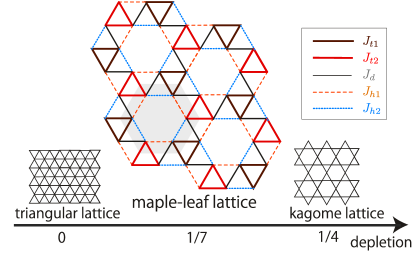
Figure 1: The relationship between triangular lattice, maple-leaf lattice, and kagome lattice and definition of exchange interaction constants. Five exchange constants of a maple-leaf lattice and the unit cell (shaded) including six sites are shown.

The geometry of the above mentioned frustrated two-dimensional lattices are interrelated; the kagome lattice can be realized by regularly depleting 1/4 of the sites of the triangular lattice. The effect of gradually weakening the interactions of the depleted sites with their surroundings is examined both for the ground state and for the thermodynamic quantitiesArrachea et al. (2004); Koretsune et al. (2009). The finite temperature double-peak specific heat and the variance of susceptibility obtained by the exact diagonalization (ED) on a small cluster indicates that the low energy properties of the two models may be smoothly interpolatedKoretsune et al. (2009). However, a more precise analysis of the excitation spectra showed that even though the Néel order is suppressed when the interaction ratio between the depleted and the regular bonds is less than 1/5, the full depletion limit of the triangular lattice antiferromagnet does not continue to the kagome lattice onesArrachea et al. (2004). These works indicate that the frustration effect depends very sensitively on the geometry of the lattice and is not easy to understand.

Here, we find another order-by-disorder phenomenon, a dimensional reduction effect, in a maple-leaf lattice antiferromagnet. The reduction of three-dimensionality of layered systems to effectively two-dimensions is previously reported both in theories and in experimentsSebastian et al. (2006); Rösch and Vojta (2007); Granado et al. (2013); Okuma et al. (2021), which is attributed to the competing frustrated inter-layer interactions. In two dimensional systems, a one-dimensional spinon-like continuum excitation is observed in a metal-organic square lattice antiferromagnetSkoulatos et al. (2017) as well as in the triangular lattice magnetColdea et al. (2003); Kohno et al. (2007). The spinon excitation in two-dimensional antiferromagnets shares the same concept as fractional chargesHotta and Pollmann (2008) or equivalently, fractons in frustrated electronic systems. However, in these systems, the dimensional reduction is encoded in the Hamiltonian; it is induced by weakening the strength of frustrated interaction associated with the reduced dimensionality, e.g. inter-layer coupling or inter-chain coupling. By contrast, in the present system, the spontaneous reduction of dimensionality occurs for a purely two-dimensional geometry of interactions. We discuss this context more precisely in §.V.

A maple-leaf lattice is a family of geometrically frustrated lattices based on a triangular unit as shown in Fig.1. It can be obtained by periodically depleting 1/7 of the sites of a triangular lattice, and is located in the diagram in between the triangular and kagome lattices. Experimental realizations of maple-leaf structure are reported both in natural mineralsFennell et al. (2011); Kampf et al. (2013); Mills et al. (2014) and in man-made crystalsCave et al. (2006); Aliev et al. (2012); Haraguchi et al. (2018, 2021). In theories, the ED study shows that the ground states of Heisenberg antiferromagnet on the maple-leaf lattice with spatially uniform interactions hosts six-sublattice long-range order similar to the one found in the classical counterpartSchulenburg et al. (2000); Schmalfuß et al. (2002). However, this long-range order may disappear when one chooses $J_{d}$ in Fig. 1 from a uniform $J$ and increase them up to $J_{d}/J>1.45$Farnell et al. (2011). These results indicate that this lattice provides another rich platform to make a comparative study of the role of geometry and the degree of frustration.

Recently, a new family member of the maple-leaf lattice called bluebellite (Cu₆I₆O₃(OH)₁₀Cl) is found to show a particular magnetic susceptibility that almost perfectly matches the Bonner-Fisher curveBonner and Fisher (1964) of a purely one-dimensional $S=1/2$ Heisenberg antiferromagnetHaraguchi et al. (2021). A similar Bonner-Fisher-like magnetic susceptibility is observed in a $S=3/2$ maple-leaf lattice antiferromagnet, Na₂Mn₃O₇Venkatesh et al. (2020). These results may suggest that there is an inherent nature in maple-leaf lattice that spontaneously reduces the dimensionality.

In this paper, we study the interplay of frustration and quantum fluctuation for this 1/7-depleted triangular lattice. In §.II we consider an antiferromagnetic Ising model and clarify the nature and the degree of frustration of the lattice. In §.III we perform an ED study and show that the ground state is a symmetry-broken stripe phase. In §.IV we examine a temperature dependence of susceptibility by varying the interaction parameters. We find that the low energy magnetic excitation shows a similar feature to that of the one-dimensional spin-1/2 XXZ model having a spin-gapped antiferromagnetically ordered ground state. By further introducing an inter-layer coupling to our model, the temperature-dependent profile of our susceptibility is modified to the one that resembles the Bonner-Fisher curve, except at a very low temperature region where our susceptibility shows an exponential decrease due to the spin-gap.

II Model

II.1 Maple-leaf lattice Heisenberg model

We consider a spin-1/2 Heisenberg model on the maple-leaf lattice with nearest neighbor interactions whose Hamiltonian is given as

$$\mathcal{H}=\sum_{\langle i,j\rangle}J_{i,j}\bm{S}_{i}\cdot\bm{S}_{j},$$ (1)

where $\bm{S}_{i}$ is a spin-1/2 operator on site $i$ and the summation is taken over all $\langle i,j\rangle$ pairs of neighboring sites. The Heisenberg model is the isotropic limit of the XXZ model given as

$$\mathcal{H}=\sum_{\langle i,j\rangle}J^{xy}_{i,j}(S^{x}_{i}S^{x}_{j}+S^{y}_{i}S^{y}_{j})+J^{z}_{i,j}S^{z}_{i}S^{z}_{j},$$ (2)

where $S^{\alpha}_{i}$ is the $\alpha=x,y$ and $z$ component of spin, and the $J^{xy}_{i,j}=J^{z}_{i,j}$ case corresponds to Eq.(1). In the following, the $J^{xy}_{i,j}$- and $J^{z}_{i,j}$-terms are often separately examined. Since this maple-leaf lattice belongs to space group $R3$, the Heisenberg spin exchange interaction $J_{i,j}$ consists of five species, $J_{t1},\,J_{t2},\,J_{d},\,J_{h1},\,J_{h2}$, whose spatial arrangement is shown in Fig. 1(a). Experimentally, in a bluebellite the structural analysis and the information on the alignment of $d$-orbials which carry spin-1/2 suggests that the sign and amplitude of these interactions are $J_{t2}\geq J_{d}\geq J_{t1}\geq J_{h1}\geq 0\geq J_{h2}$. Whereas, for simplicity and to clarify the intrinsic nature of the geometry of lattice, we set $J_{t1}=J_{t2}=J_{d}=J,$ $J_{h1}=-J_{h2}=J_{h}$ and vary $J_{h}/J$ as a parameter in the main part of the calculation. We denote the total number of sites as $N$ and the number of unit cells as $N_{\rm cell}$, where $N=6N_{\rm cell}$ for the maple-leaf lattice and $N=7N_{\rm cell}$ for the corresponding triangular lattice.

II.2 Ising limit

We first examine the nature of frustration of the maple-leaf lattice through the comparison with the triangular lattice. To this end, consider an Ising model which is the classical limit of the Heisenberg model, where the quantum fluctuation due to spin exchange is neglected by taking $J^{xy}_{i,j}=0$ in Eq.(2).

Let us remind that the ground state of an antiferromagnetic Ising model on a uniform triangular lattice with $J^{z}_{ij}=J>0$ consists of massive numbers of states which altogether contribute to the residual entropy amounting to $S=0.323k_{\mathrm{B}}N$Wannier (1950). The local constraint of Ising spins that belong to this degenerate ground state is to have either two-up one-down spins or two-down one-up spin on a triangle; the state is called UUD/DDU, whose Ising energy is $E_{\rm ising}=-NJ/4$.

To see how the lattice geometry changes the low energy structure of the model, we gradually vary the strength of $J_{\rm maple}$, which are the six bonds inside the hexagon to be depleted where $J_{\rm maple}=0$ corresponds to the full 1/7-depletion of the triangular lattice. As shown in Fig. 2(a) the UUD/DDU states split into several levels with equal energy spacings, $E_{\rm ising}=-J(N/4-n)-J_{\rm maple}n$, where $n=0,1,...,N/7$, while the energy of the lowest level remains unchanged.

For a 1/7-depleted structure at $J_{\rm maple}=0$ we can further decrease the strength of bonds around the depleted hexagon as $J_{h1}=J_{h2}=1$ to 0, as shown in Fig. 2(b), where all the UUD/DDU levels vary linearly as $E_{\rm ising}=-J(N/24+n)+J_{h}(2n-N/4)$ where $n=0,1,...,N/6$, and all the UUD levels cross at $J_{h1}=J_{h2}=0.5J$ which has a comparably large degeneracy with the original triangular lattice. Finally, in Fig. 2(c) we introduce the alternating ferromagnetic and antiferromagnetic bonds along the hexagon and increase their amplitude, finding that all the UUD/DDU levels remain unchanged. The higher energy levels shown in broken lines are the non-UUD states, namely their UUD/DDU structure is partially broken. With increasing $\pm J_{h}$, they descend and overtake the perfect UUD/DDU at $J_{h1}=-J_{h2}\geq 0.5$. The parameter used in Fig. 2(c) is the one we mainly focus on.

The frustration generated by the competition between different exchange interactions usually leads to large classical ground-state degeneracies. In the present case, the upper bound of the degeneracy of the lowest energy UUD/DDU manifold for $J_{h1}=J_{h2}(>0.5)$ is roughly evaluated as $2^{N/6}$ with a corresponding residual entropy of $S=0.116k_{\rm B}N$, and for $J_{h1}=-J_{h2}$ as $6^{N/6}$ with $S=0.299k_{\rm B}N$, which are explained as follows. In the former antiferromagnetic $J_{h}$, the lowest energy UUD/DDU states satisfy the condition that the spins align in a staggard manner along the hexagons to maximally gain $J_{h}$. For each hexagon, one can prepare two such states, which give $2^{N/6}$. However, among them, those giving UUU or DDD configurations to $J_{t1}$ or $J_{t2}$ triangles should be excluded. For three adjacent hexagons, 2 states among $2^{3}$ are excluded, while for four adjacent hexagons, again 2 states among $2^{4}$ are excluded, which means that the lower bound of degeneracy is still as large as $2^{N/6}(3/4)^{N/6}$ leading to the massive residual entropy.

In the latter case, the local constraint for the lowest energy UUD/DDU states is to have both sides of spins on $J_{d}$ bond align antiparallel. Therefore, once the UUD/DDU spin configurations on $N/6$ different $J_{t1}$-triangles are determined, the spin configurations on all $J_{t2}$ triangles, namely the whole rest of the spins are automatically determined through $J_{d}$ bonds. Among them, those giving UUU/DDD to $J_{t2}$ triangle should be excluded. For three adjacent $J_{t1}$ triangles, among $6^{3}$ UUD/DDU states the ones that give UUU/DDD on $J_{t2}$ enclosed by these three is 54. Therefore, the lower bound of degeneracy is $6^{N/6}(162/216)^{N/6}$. Notice that for both cases, the lowest UUD/DDU manifold includes the state outside the UUD/DDU manifold of the triangular lattice, and the former is not the subspace of the latter, as we discuss shortly.

Another quantitative measure of frustration given by Lacorre Lacorre (1987) is the constraint function $F_{c}=-E_{0}/E_{b}$ where $E_{0}$ is the ground state energy and $E_{b}=-\sum_{\langle i,j\rangle}|J^{z}_{ij}|(S_{i}^{z}S_{j}^{z})_{\rm max}$. When $F_{c}=-1$ all the local bond energies are optimized simultaneously and there is no frustration, whereas $F_{c}\sim 0$ means that the competition of local interaction leads practically to no energy gain. As shown in the lower panels of Fig. 2(a)-(c), $F_{c}$ first decreases and becomes less frustrated in depleting $J_{\rm maple}$. With tuning the sign and values of $J_{h}$, it becomes as frustrated as the original triangular lattice Ising model, e.g. when $J_{h1}=-J_{h2}=J$ or $J_{h1}=J_{h2}=J/2$.

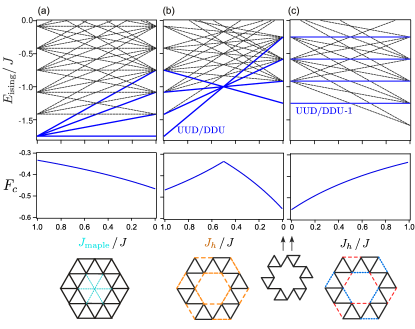
Figure 2: Ising energy $E_{\rm ising}=\langle{\cal H}_{\rm ising}\rangle/N_{\rm cell}$ per unit cell for the lowest few levels in the $S_{z}^{(\mathrm{tot})}=0$ sector obtained for 18 site cluster by varying the geometry of the lattice. Here, we introduce $J_{\rm maple}$ which are the six bonds inside the hexagon depleted in constructing the maple-leaf structure from a triangular lattice. (a) $J_{\rm maple}$ varied by fixing $J=J_{t1}=J_{t2}=J_{d}=1$ (antiferromagnetic), (b) $1\geq J_{h1}=J_{h2}\geq 0$ (antiferromagnetic) varied by taking $J_{\rm maple}=0$, where $J_{h1}=J_{h2}=0$ on the r.h.s. has the structure consisting of triangles connected with each other by a single bond $J_{d}$. (c) $J_{h1}=-J_{h2}\geq 0$ around the hexagon consisting of antiferromagnetic and ferromagnetic bonds is varied which is the structure we mainly focus on. For all panels, the solid lines correspond to the UUD/DDU states and the broken lines are the states with UUD/DDU partially violated. The constraint parameter $F_{c}$ is examined, where $F_{c}=-1$ corresponds to the nonfrustrated case and $F_{c}\sim 0$ to the highly frustrated limit.

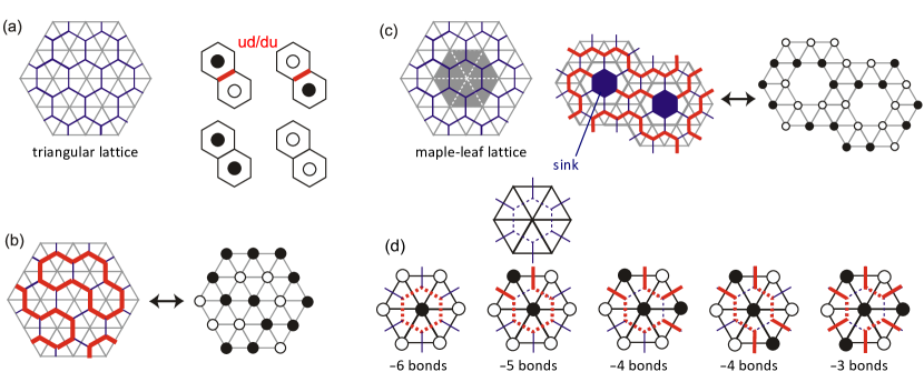
Figure 3: (a) Relationship between the triangular lattice (gray lines) and its dual lattice (blue lines). Red bold bonds are placed on the honeycomb bond which crosses the up-down pairs of spins on the triangular lattice. (b) One of the examples of the UUD/DDU structures on a triangular lattice described by the fully packed loop model on a honeycomb lattice. (c) Correspondence of the maple-leaf lattice and its dual lattice, a honeycomb lattice with sinks. The two right panels are the example of the loop-string model on the honeycomb lattice with sinks and the corresponding UUD state of the maple-leaf lattice. (d) All the UUD/DDU patterns on the hexagonal unit around the depleted site. Broken bonds are part of the loops to be depleted, where the number of these bonds distribute between -6 to -3.

To give an intuitive understanding of the above mentioned behavior of low energy levels, we introduce a dual lattice description of the model. Figure 3(a) shows a honeycomb lattice which is a dual lattice of the triangular lattice. One can map the UUD/DDU states of a triangular lattice to the fully packed loop-covering states on a honeycomb lattice in the following manner; when the neighboring two spins on a triangular lattice is antiparallel, the edge of the dual lattice in between these spins is filled by a bold red bond. Since each triangle has two antiparallel pairs of spins, there is a local constraint that each honeycomb site is connected to two red bonds, and resultantly this red bond always forms a closed-loop while never cross with each other (see Fig. 3(b)). By counting the total length of the loops the Ising energy is obtained, which takes a maximum, i.e. $2N$, for the UUD state. A fully-packed loop model is spanned by the restricted Hilbert space consisting only of these loop states and serves as a low energy effective model of strongly correlated quantum spin and charge systems on a triangular lattice and kagome lattices Pollmann et al. (2014).

Depleting 1/7-sites from the triangular lattice modifies the nature of loops on its dual lattice. Figure 3(c) shows the dual lattice of the maple-leaf lattice, where the honeycomb lattice is modified such that the hexagons of the honeycomb lattice surrounding the depleted triangular sites are erased. We call this vacant unit hexagon a “sink”. Since the center triangular site is depleted, the hexagonal bonds surrounding the sink are never filled by loops or bonds. Then, some of the fully packed loops of a honeycomb lattice that crossed the sink can no longer form a closed loop, and their open edges enter the sink. We call this description a fully packed loop-string state, whose example is shown in the right panel of Fig. 3(c). Due to this modification, the total length of the loops and strings are not necessarily the same although they all describe the UUD/DDU state of the maple-leaf lattice. Namely, the length of the loop and string varies according to the number of loop-bonds that belonged to the sink and are lost by depletion. This splits the originally degenerate ground-state manifold of the triangular lattice model into equally spaced hierarchial energy levels (see Fig. 2). As shown in Fig. 3(d), the number of depleted red broken bonds is between 3 to 6. Each depleted bond carries $0.25J_{\rm maple}$ and the energy level spacing amounts to $0.5J_{\rm maple}$ per six-site unit cell(see Fig. 1).

In a maple-leaf lattice, the Ising energy further changes by varying the bond strength along the hexagon $J_{h1}=\pm J_{h_{2}}>0$ while keeping $J_{t1}=J_{t2}=J_{d}=J$. For each sink, even number of strings enter which we denote as $2d$ with $d=0,1,2,3$. The bonds lost by depletion are shown in broken lines in Fig. 3(d). Their number is given as $6-d$, and the $2d$ bonds carry $\pm J_{h}/4$ instead of $-J/4$. When all the bonds are antiferromagnetic as $J_{h2}=J_{h}>0$, the Ising energy for each level in Fig. 2(b) measured from the classical Ising energy on the triangular lattice is given as $E_{\rm ising}=\sum_{i}(6-2d_{i})J/4+(-J_{h}+J)(d_{i}-3/2)$ and depend on $J_{h}$. However, when half of the bonds on the hexagon is ferromagnetic as $J_{h2}=-J_{h}<0$, the contribution from the hexagons are canceled out and we find a $J_{h}$ independent profile of energy $E_{\rm ising}=\sum_{i}(6-2d_{i})J/4+J(d_{i}-3/2)$ in Fig. 2(c); as shown in Fig. 4(a) we need to assign different colors to six bonds that may cross the edges of the sink, which contribute to the Ising energy as $\pm J_{h}$. Then, for all five different configurations of strings entering the sink shown in Fig. 4(b) the number of green and red colored bonds are always equal, which is the reason for the cancellation.

We finally mention that there are other non-negligible states that belong to the UUD/DDU states of the maple-leaf lattice but do not continue to the UUD/DDU states of the triangular lattice. One example is shown in Fig. 4(c). The three up spins and three down spins form neighbors around the hexagon of a triangular lattice whose center spin is to be depleted. In this case, two triangles inside the hexagon are either UUU or DDD, regardless of the orientation of the center spins. However, these triangles are wiped out by the depletion. Therefore, the UUD states of the maple-leaf lattice are not the subspace of the UUD states of the triangular lattice. We show in Appendix A that the Ising energy of such additional UUD/DDU states on a maple-leaf lattice also remains unchanged in varying $J_{h1}=-J_{h2}$.

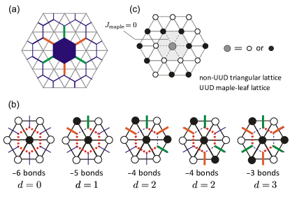
Figure 4: (a) Assigning two different colors to the edges leading to the sinks. Red and green lines denote the antiferromagnetic $J_{h}$ and ferromagnetic $-J_{h}$. (b) Five UUD/DDU patterns on the hexagonal unit around the depleted site with $d=0,1,2,3$, where $2d$ is the number of edges of loops that enter the sink. Broken lines are part of the loops inside the sink that disappear due to depletion, which amount to $6-d$. (c) UUD/DDU states on the maple-leaf lattice which were originally a non-UUD/DDU states of the triangular lattice. Inside the hexagon, we have UUU or DDD triangles.

III Ground state

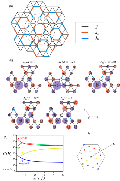
Figure 5: (a) Maple-leaf lattice and 18-site finite-size cluster with periodic boundary conditions. (b) Spin-spin correlation functions , $\langle S_{1}S_{j}\rangle$, between site 1 and site j of a ground state for several choices of $J_{h}/J$ obtained by ED. The area of each circle is proportional to the magnitude of $\langle S_{1}S_{j}\rangle$, with red/purple ones being positive/negative (ferromagnetic/antiferromagnetic). (c) Spin structural factor $C(k)$ in Eq.(3) calculated for $N=18$ cluster. The $k$-points inside the Brillouin zone of the maple-leaf lattice are shown in different symbols which are classified into five groups based on $R3$ space group. We have $\bm{k}=(4n-m)/21(1,-1/\sqrt{3})+(5n-4m)/21(0,2/\sqrt{3})$ with representative data points as $(n,m)=(1,1)$ for stripe (red bullet), $(0,\pm 1)$ (yellow star), $(0,\pm 2)$ (green pentagon) and $(\pm 1,\mp 3)$ for windmill type (blue diamond). The temperature dependences of $C(k)$ is obtained by taking an average of over 50 realizations of the TPQ state(see Section IV for details).

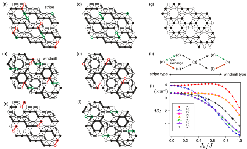
Figure 6: (a)-(g) Representative configuration of spins belonging to UUD/DDU-1 states that give major contribution (large $w_{l}$) to the ground state wave function. (a) Stripe and (b) windmill states are the most symmetric ones. Panel (h) shows the relationships between states (a)-(g); states (c) and (d) can be obtained from (a) by periodically exchanging the nearest neighbor up and down spins on green and red bonds, respectively. States (e) and (f) can be obtained from (b) in the same manner. In panel (i) we plot the actual weights $w_{l}$ of states (a)-(g) as functions of $J_{h}/J$ when $J_{h1}=-J_{h2}=J_{h}$. At $J_{h}/J=1$ there appears some non-UUD configurations having larger $w_{l}$ than the (b), (e), (f), and (g) states.

In this section, we numerically analyze the Heisenberg Hamiltonian Eq.(1) and show that the unique stripe ground state is possibly formed by the order-by-disorder effect from the lowest UUD/DDU states of the Ising limit of the maple-leaf lattice we discussed in the previous section.

III.1 Exact diagonalization

We first perform an exact diagonalization (ED) for $N=18$ clusters with periodic boundary conditions (see Fig. 4(a)) and obtain the ground state of the maple-leaf lattice. As we see shortly, the extended magnetic unit cell has 18-sites, and the larger size available $N=24,30$ do not match this unit. This mismatch artificially destabilizes some of the magnetic structures, which we want to avoid. Choosing $N=18$ enables the full classification of basis states which is convenient to examine their stability in an unbiased manner. We additionally examined the $N=24$ ground state in parallel and confirmed that the major conclusions obtained for $N=18$ do not change which we explain in the final part of this section. To understand the magnetic property of the ground state we calculate the correlation function and obtain a structural factor,

$$C(\bm{k})=\frac{1}{N}\sum_{i,j=1}^{N}e^{ir_{ij}k}\langle S_{i}S_{j}\rangle.$$ (3)

We first show in Fig. 5(b) the correlation functions, $\langle S_{1}S_{j}\rangle$, in a bubble chart, where the area of the bubble indicates the strength of the correlation. A stripe pattern develops along 15-17-(1-)2-3-5-6-15 for all values of $0<J_{h}/J<1$, and 9-(8-)18-17-2-12-11-9 for $J_{h}/J\approx 1$. The correlation between site 1 and site 17 is the most prominent but becomes weaker by increasing $J_{h}/J$, and at $J_{h}>J/2$ the inequivalence of the magnitude of the correlation between sites becomes smaller. This tendency is consistent with the Ising energy diagram of Fig. 2(c) where at $J_{h}>J/2$ the non-UUD excited states become the lowest.

Figure 5(c) shows the structural factor in Eq.(3), where the $\bm{k}$-points are the discretized reciprocal points for the $N=18$ cluster. The $\bm{k}$-points inside the Brillouin zone can be classified into five groups, depending on the symmetry of the system. One finds that the peak at $\bm{k}=(2\pi/7,10\sqrt{3}\pi/21)$ shown in red bullet which originates mainly from the stripe-type correlation dominates the ground state. This tendency lasts up to $k_{B}T/J\lesssim 0.5$ (for the details of the calculation, see the next section), which is the peak position of the susceptibility we see shortly. The same tendency is observed for other values of $J_{h}/J$.

To understand the underlying mechanism for the development of one-dimensional-like correlation, we examine the types of basis that have a major contribution to the ground state wave function, $\ket{\mathrm{GS}}=\sum_{l}c_{l}\ket{l}$. It is spanned by the total-$S_{z}=0$ space, $\{\ket{l}\}$ of $l=1,...,\,_{N}C_{N/2}$, which are the classical Ising spin configuration we discussed earlier. Several series of states $\ket{l}$ having large weights $w_{l}=|c_{l}|^{2}$ are extracted; we select totally 102 basis states in descending order of $w_{l}$, which are classified into seven groups of states. Their representative configurations are shown in Figs. 6(a)-6(g). Within each group, the states are related by the $\pm 2\pi/3$ rotational and spin inversion symmetries (not shown). The stripe pattern (a) is one-dimensional and the windmill pattern (b) is a regular two-dimensional UUD/DDU configuration. The relationships between these seven groups of states are summarized in Fig. 6(h); types-(c) and (d) can be obtained from type-(a) by exchanging one nearest neighbor pair of spins per 18 sites periodically, which are marked by green and red bonds. Types-(e) and (f) can be obtained from type-(b), and finally type-(g) with the lowest symmetry can be obtained from types-(c), (d), (e) and (f) by the same process. In this sense, types-(c) and (d) are similar to (a) and are called stripe-type, (e) and (f) are similar to (b) and are the windmill-type.

The weights $w_{l}$ of states (a)-(g) as functions of $J_{h}/J$ are shown in Fig. 6(i). The relationships between them are understood as follows: for $J_{h}/J=0$, (a) stripe and (b) windmill have the same weight, and (c), (d), (e), (f), and (g) have the same weight as well. By introducing $J_{h}$, the stripe (a) and its analogs (c) and (d) dominate the ground state which continues for $0\leq J_{h}/J\leq 1$. The second highest contributing configuration is (b) for $0<J_{h}/J\lesssim 0.37$, but it is overtaken by the stripe-type (c) and (d) for larger $J_{h}$. At $J_{h}/J=1$, although the stripes (a), (c) and (d) continue to have the largest $w_{l}$, the other non-UUD type of spin configurations suddenly become dominant compared to (b) and other windmill types of states.

In viewing this characteristic feature of the ground state by restarting from the classical Ising limit, even though we introduce the quantum fluctuation effect, $J^{xy}_{i,j}$-term in Eq.(2), the major contribution to the ground state is still a series of UUD/DDU states for all values of $0\leq J_{h}/J\leq 1$. In fact, the states (a)-(g) in Fig. 6 all belong to the lowest UUD-manifold of states called UUD/DDU-1 of Fig. 2(c) with $E_{\rm ising}/J=-5N/24$. At $J_{h}/J\geq 1/2$, the other non-UUD states have the lowest Ising energy, whereas in the Heisenberg model, the full UUD/DDU states overwhelm the non-UUD states due to the energy gain from the quantum fluctuations.

III.2 Energy Gain

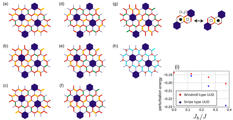
Figure 7: (a)-(g) Bond configurations on the dual lattice corresponding to (a)-(g) in Fig. 6. Edges shown in yellow/green lines ($J_{d}$) are always occupied with bonds in these manifolds and spin-exchange around a yellow line yields another UUD configuration having the same classical energy while that around a green line does not. (h) All the yellow/green bonds in (a)-(g) are shown here in the same colored bonds. A bond configuration can be determined by identifying bond tilings on the edges connected to the vertices (orange dots) in this manifold. (i) Energy gain at the second-order of ${\cal H}_{xy}$ where all the processes of going into other manifolds from UUD/DDU-1 and coming back are considered.

To understand the reason why the stripe ground state is realized, we examine the effect of quantum fluctuations on the Ising UUD states. We start from the Ising model and introduce ${\cal H}_{xy}=J^{xy}_{i,j}(S_{i}^{+}S_{j}^{-}+S_{i}^{-}S_{j}^{+})/2$ by setting $J^{xy}_{i,j}$ much smaller than the Ising interaction $J^{z}_{i,j}$ in Eq.(2). We first rewrite the UUD/DDU configurations in Fig. 6 (a)-(g) using the loop-string model on the dual lattice as shown in Fig. 7(a)-(g). As mentioned earlier, the UUD/DDU structures correspond to the fully packed states of loops and strings. Since the length of the loop-string is the number of pairs of neighboring up and down spins, the fully packed loop-string states are maximally flippable in overall and may gain $E_{q}=\langle{\cal H}_{xy}\rangle/N_{\rm cell}$ the most compared to other classical Ising states. In this context, the ones in Fig. 7(a)-(g) have an equivalent length of loops and may equally contribute to the ground state. However, in reality, the way how ${\cal H}_{xy}$ works differs between these seven groups of states.

We focus on UUD/DDU-1 and operate one of the ${\cal H}_{xy}$-terms to this manifold. If we obtain a state that again belongs to UUD/DDU-1, this term mixes the states within the UUD/DDU-1 manifold at the first order of $J^{xy}_{i,j}$. If a term in ${\cal H}_{xy}$ transforms the UUD/DDU-1 to the state outside this manifold, by operating a proper ${\cal H}_{xy}$-term again, we may come back to the UUD/DDU-1 state; this process serves as a second-order perturbation.

We first consider the first-order perturbation. The right panel (inset) of Fig. 7 shows the exchange process of antiparallel spins between a pair of nearest neighbor sites $\langle i,j\rangle$ and a pair of hexagons on the dual lattice surrounding the two spins. The center vertical bond shared by the $\langle i,j\rangle$ hexagons remains unchanged, whereas occupation of bonds on the other four edges of each hexagon is converted from unoccupied to occupied or vise versa. This is because if the spin on $i$-th site flips up-side-down, the ferromagnetic neighbor becomes an antiferromagnetic one and vise versa.

In Figs. 7(a)-(g), we classified the color of occupied bonds that belong to the loop-string into red, yellow and green. The yellow and green bonds are the $J_{d}$-bonds.

The UUD/DDU-1 are characterized as those having all these yellow and green bonds to be occupied. When we flip the spins on yellow bonds, the number of occupied bonds, namely the number of red bonds associated with this process remains unchanged, and the UUD/DDU-1 state stays within the UUD/DDU-1 manifold. Therefore, we call this yellow bond a flippable bond (see Appendix B). The two structures, stripe-(a) and windmill-(b) have the maximum number of yellow bonds amounting to 2/3 of the flippable bonds while other structures only have 4/9 of them. This means that stripe and windmill-states gain the energy the most at the first-order perturbation by maximally mixing with other UUD/DDU-1 states.

As for the green bond, the spin-exchange will transform the UUD/DDU-1 state to the non-UUD/DDU states outside the manifold. In Fig. 7(i), we evaluated the second-order perturbation energy gain by starting from the windmill or stripe-state, operating ${\cal H}_{xy}$ twice and summing up the energy gain from each process where we set $J^{xy}_{i,j}=J_{i,j}$ for simplicity. When $J_{h}/J>0$, the stripe state becomes more stable than the windmill state. Flipping the spins on red bond also transforms the UUD/DDU-1 state outside the manifold and can be treated the same as the green bond.

To be precise, the way how ${\cal H}_{xy}$ mixes the low energy states is more complicated including not only the UUD/DDU-1 but other UUD/DDU’s and the non-UUD/DDU state. Still, the above discussion gives an overall intuitive understanding that the stripe-order appears due to the quantum order-by-disorder effect from the classical degenerate UUD/DDU-1 manifold of states.

We finally mention that the $N=24$ cluster which is larger than the $N=18$ we adopted, does not accommodate the windmill and stripe type of structures. However, in calculating the ground state for $N=24$ we find that the overall tendency obtained for $N=18$ remains unchanged; the UUD/DDU-1 manifold dominates the ground state, and the largest contribution to the ground state is the irregular stripe even though the shape of the stripe is modified due to the mismatch of the shape of the cluster.

IV Finite Temperature

The ground state of this model possibly breaks the translational symmetry of the original lattice, and form a stripe type Néel order. To understand the relevance of this ground state with the characteristic behavior of the magnetic susceptibility resembling those of the one-dimensional Bonner-Fisher curve, we calculate the finite temperature properties of the model. Here, we apply a thermal pure quantum (TPQ) method using $N=18,24$, and 30 clusters. Similarly to finite-temperature ED methodsJaklič and Prelovšek (1994); Aichhorn et al. (2003); Hams and De Raedt (2000), this method gives thermodynamic quantities at finite $N$ by few sample averagesSugiura and Shimizu (2012). Starting from the high-temperature random state prepared based on the Haar measure, $|0\rangle=\sum_{i}C_{j}|j\rangle$, where $C_{j}$ is a random complex coefficient and $\{\ket{j}\}$ is the Fock space of a finite size lattice, and successively operating the Hamiltonian $(l-{\cal H}/N)$ shifted by a constant $l$, a series of states $|k\rangle=(l-{\cal H}/N)^{k}|0\rangle$ that represent the thermal equilibrium at different temperatures are obtained. By using these series of states, we obtain a magnetic susceptibility. We took more than 30 sampling averages for $N=24$ while for $N=30$ which is the size large enough to represent the thermal state without random average we used a single calculation.

IV.1 Magnetic susceptibility

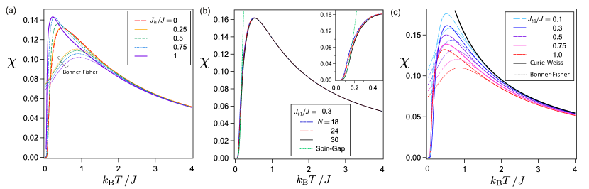
Figure 8: (a) Uniform magnetic susceptibility $\chi$ for several choices of $J_{h1}=-J_{h2}=J_{h}$ with $J_{t1}=J_{t2}=J_{d}\equiv J=1$. (b) $\chi$ obtained for $N=24$ and 30 with $J_{t2}=J_{d}=1,J_{h1}=-J_{h2}=0.1$ and $J_{t1}=0.3$. Inset shows the magnified $\chi$ at low temperature. (c) $\chi$ for several choices of $J_{t1}/J$ with $J_{t2}=J_{d}=1$ and $J_{h1}=-J_{h2}=0.1J$. The solid bold line is the Curie-Weiss susceptibility $\chi_{cw}=J^{cw}/4k_{B}(T-\Theta)$ with $J^{cw}=0.928$, $\Theta=-0.396$, whose values are obtained by fitting $\chi$ for $J_{t1}=0.1J$. Broken lines in both panels (a) and (c) are the Bonner-Fisher susceptibility whose parameter $J^{1d}$ is adjusted to fit to the susceptibility of the maple-leaf lattice for each parameter.

First we set $J_{t1}=J_{t2}=J_{d}=J$, $J_{h1}=-J_{h2}=J_{h}$ as we did for the ground state. A uniform magnetic susceptibility $\chi$ of a $N=24$ cluster for various choices of $J_{h}$ is shown in Fig. 8(a). At low temperature, we find $\chi\propto(\Delta/k_{B}T)^{1/2}e^{-\Delta/k_{B}T}$ basically for all choices of $J_{h}/J$, which indicates a spin-gapped ground state. For a finite cluster calculation, a fictitious spin gap of order $\Delta\sim 1/\sqrt{N}$ often appears as an artifact of finite size effect. To examine whether the observed gapped behavior is an intrinsic property of the model, we compared the result of $N=30$ cluster with $N=18,24$ ones in Fig. 8(b). The magnitude of spin gap extracted by fitting $\chi$ at low-temperature yields $\Delta\sim 0.507(N=24)$ and $0.588(N=30)$, which increases with $N$. For the temperatures above the peak position, the difference of $\chi$ between the two system sizes is almost negligible. From these results, one can judge that the spin gap is finite.

Although several experimental measurements on the maple-leaf materials suggest that the measured $\chi$ follows a Bonner-Fisher curve characteristic of a gapless one-dimensional Heisenberg antiferromagnet, our result with a spin-gapped ground state does not conform to such correspondence. In Fig. 8(a), we plotted together with the Bonner-Fisher curve by adjusting its Heisenberg interaction $J^{1d}$ to fit the high temperature ($k_{\mathrm{B}}T>1.5J$) tail of $\chi$ to the ones of the maple-leaf lattice. For all cases, $\chi$ of the two models do not agree at $k_{B}T\lesssim J$. In fact, $\chi$ develops toward lower temperatures than the Bonner-Fisher ones with the higher peaks at lower temperatures. Such development of peak is the characteristic feature of the two-dimensional highly frustrated antiferromagnet, e.g. a kagome lattice onesHotta and Asano (2018).

To show that this conclusion is not due to our specific choices of parameters, we examine overall variations of parameters of the model. Particularly, we investigate the small $J_{h}/J$ region, where the two $\chi$’s have relatively better correspondence. Figure 8(c) shows the case where one of the triangular units $J_{t1}$ is varied while other parameters are fixed to $J_{t2}=J_{d}=J$, $J_{h1}=-J_{h2}=J_{h}=0.1J$. Note that the properties of an Ising energy diagram and ground state described in Sec. II and III hold for these choices of parameters. Again although we properly adjusted $J^{1d}$ for the Bonner-Fisher plot, the two models do not give a consistent $\chi$ in its amplitude. However, the peak position becomes closer to each other by decreasing the parameter down to $J_{t1}/J\sim 0.1$ As a reference we also show the Curie-Weiss susceptibility $\chi_{cw}=J^{cw}/4k_{B}(T-\Theta)$ with $J^{cw}=0.928$, $\Theta=-0.396$ for the same spin density as the maple-leaf lattice to compare with other $\chi$.

IV.2 One dimensional magnon propagation and the XXZ model

The spin gap and the enhancement of $\chi$ indicate that the low energy effective model of the maple-leaf lattice is not a uniform antiferromagnetic Heisenberg chain. However, there is another model, an XXZ model that has a finite spin gap an enhanced susceptibility, the absence of finite temperature phase transition and the symmetry-breaking long-range Néel ordered ground state. All these features do not contradict the results we obtained for the present system.

We thus compare the susceptibility of the one-dimensional antiferromagnetic XXZ model,

$$\mathcal{H}_{1d}=\sum_{i}J^{1d}_{xy}(S^{x}_{i}S^{x}_{i+1}+S^{y}_{i}S^{y}_{i+1})+J^{1d}_{z}S^{z}_{i}S^{z}_{i+1},$$ (4)

where besides $J^{1d}_{xy}$ one can adjust $J^{1d}_{z}>J^{1d}_{xy}$ to fit the susceptibility as well as the spin gap. The temperature dependence of $\chi$ is obtained by a size-free calculation using a sine-square deformation combined with the TPQ methodHotta and Asano (2018) which gives $\chi$ of the thermodynamic limit.

As shown in Fig. 9(a), the profile of $\chi$ with smaller $J_{t1}/J$ can be fitted well with magnetic susceptibility of one-dimensional XXZ model for all temperature regions. Here, we obtain $J^{1d}_{xy}=0.465$, $J^{1d}_{z}/J^{1d}_{xy}=2.25$ and $\Delta=0.581$ for the XXZ model (see Fig. 9(b)) which is the exact solution of a spin gap of Eq.(4) that gives the best fitting.

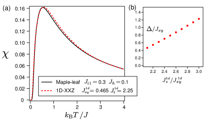
Figure 9: Magnetic susceptibility with $J_{t2}=J_{d}=1$, $J_{t1}=0.3$, and $J_{h1}=-J_{h2}=0.1$ compared with the magnetic susceptibility of XXZ model with $J^{1d}_{z}/J^{1d}_{xy}=2.25$, where $\Delta=0.54$ .

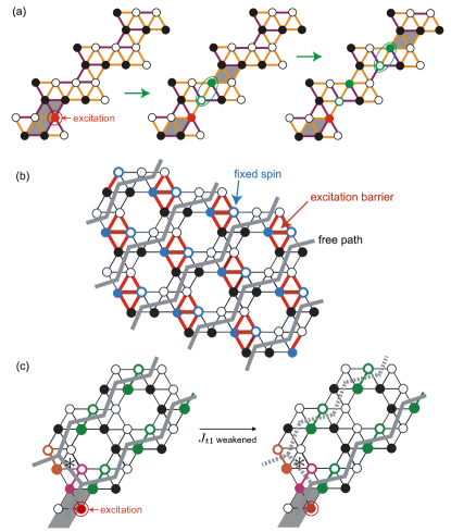
Figure 10: (a) Example of magnon excitation from a stripe. A red bullet marked with a circle denotes the location of the excited spin, and the adjacent two shaded plaquettes is a magnon that separates into two spinons. When ${\cal H}_{xy}$ is operated, the up and down pairs of spins on a green bond marked with oval exchanges and a spinon (shaded plaquette) hops to the upper right by one lattice spacings. These spin exchanges do not change the Ising energy. Bonds gaining/losing energy are shown in orange/purple lines. (b) Schematic illustration for the spinon propagation rules. Blue open circle indicates the spins that rarely contribute to the spin-exchange process (fixed spin) since a finite Ising energy loss occurs. Propagation in the direction across the red lines is energetically disadvantageous, and the direction that keeps the Ising energy unchanged is restricted to those along the gray lines. (c) Path marked with star denotes the exceptional propagation of spinon through exchanging orange and red spins, which appears only when the magnon is excited on a particular site marked with a circle. Weakening $J_{t1}$ from the left panel to the right, weakens the connection through starred path and strengthen the one-dimensionality.

To understand the origin of the coincidence between $\chi$’s of the two models, we examine a single magnon excitation of the maple-leaf lattice. For simplicity, we consider a classical stripe UUD/DDU-1 configuration which gives a dominant contribution to the ground state of the Heisenberg model. Figure 10(a) shows the example of how the excited magnons propagate by the spin-exchange process, ${\cal H}_{xy}$. To identify the location of magnons we use a pair of shaded plaquettes consisting of four triangles extending in the upper-right direction. When the system is in the UUD/DDU state such plaquettes are magnetically neutral (unshaded) since we always have even numbers of up and down spins. By flipping a down spin to up, the two plaquettes sharing that site are magnetized as UUUD, which host one magnon. Unlike the standard Ising models, the spin-exchange that keeps $E_{\rm ising}$ unchanged takes place, not at the neighboring bonds of the excited magnon site, but at the next nearest neighbor, i.e. it is the neighboring bond of the shaded plaquette. By the exchange of two spins marked with ovals in Fig. 10(a), one of the plaquettes hops to the upper-right by two lattice spacings. The same operation will propagate the plaquettes in the upper-right or lower-left directions along the stripe. Since the two-plaquettes share one magnon, and since this propagation separates two plaquettes freely along the one-dimensional direction at the first-order level of ${\cal H}_{xy}$, each shaded plaquette is regarded as spinon. In the one-dimensional antiferromagnetic XXZ model or Ising model, a similar spinon excitation is observed above the spin gap, and this would explain the resemblance of $\chi$ between the two models.

The one-dimensionality of this spinon propagation is confirmed as follows. There is a relatively larger energy cost of flipping the spins marked with blue-open symbol in Fig. 10(b); its Ising energy gain with its surroundings amount to $-(J_{d}+2J_{t1})/4$ or $-(J_{d}+2J_{t2})/4$, larger than for the other spins $-J_{d}/4$ that join the spinon propagation. Accordingly, the exchange of spins marked with solid and open blue circles have a large energy loss of $(J_{t1}+J_{t2})/2$, and work as a spatial barrier. There are two barriers per every depleted hexagon, which restrict the propagation of magnons to a one-dimensional direction in the gray line.

There is an exceptional case that may slightly allow the two-dimensional propagation; in Fig. 10(c) the path marked with the star had an energy barrier in the stripe UUD state but once a magnon is excited on a particular site indicated by an arrow, the energy barrier is lost and the magnon can propagate by exchanging spins on the orange and pink bonds. However, the energy barrier is lost only for the limited choices of excitation, and the overall nature of the magnon propagation is regarded as one-dimensional. A smaller $J_{t1}/J$ weakens the connection through the starred path because $J_{t1}$ is responsible for the energy gain due to the exchange of spins on the orange bond. Consequently, the smaller $J_{t1}/J$ strengthens the one-dimensionality of the propagation pathway. This may explain the reason why our magnetic susceptibility with smaller $J_{t1}$ gives better correspondence to the ones for the one-dimensional XXZ model.

As can be understood from the similarities of the nature of the magnetic excitations, the dimensional reduction is expected only for the magnetic properties of the system. We examined the specific heat of the two models for the same parameters in Appendix D, and found that the nonmagnetic part of the low energy excitations differs between the two models. Whereas, the onset of the magnetization curve of the maple-leaf lattice (see Appendix D) shows a criticality reminiscent of the gapped 1D spin system, which is another sign of the dimensional reduction effect. The parameter range that the dimensional reduction is observed is limited to the case of small $J_{h1}=-J_{h2}$. For all antiferromagnetic $J_{h1}=J_{h2}>0$, the system recovers a two-dimensional Néel ordering (see Appendix E).

IV.3 Three dimensionality due to inter-layer coupling

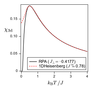
Figure 11: Magnetic susceptibility $\chi_{\rm 3d}$ with $J_{t2}=J_{d}=1,J_{h1}=-J_{h2}=0.1$ and $J_{t1}=0.30$ considering interplanar interaction $J^{\prime}=-0.4177$ with RPA. Broken line is the Bonner-Fisher curve of a one-dimensional Heisenberg model.

In the previous subsection, we figured out that the susceptibility of the maple-leaf lattice can be fitted well throughout the whole temperature range by the one-dimensional XXZ model with appropriate choices of the ratio of $J_{z}/J_{xy}$ as well as $J_{xy}$ that also reproduces a finite spin gap of the ground state. Compared to the Bonner-Fisher curve for the one-dimensional Heisenberg model, these susceptibilities show large enhancement toward low temperature with higher peaks.

On the other hand, the experimental observation indicates that for bluebellite the susceptibility shows almost perfect coincidence with the Bonner-Fisher curve down to temperatures just below the peak positionHaraguchi et al. (2021). In further lowering the temperature, there occurs a phase transition in experiments to the Néel ordered state due to the three-dimensionality of the material, which masks the intrinsic low-temperature property of the purely two-dimensional magnet.

Here, we examine whether our XXZ-like susceptibility may reproduce the Bonner-Fisher curve except at temperatures lower than the spin gap. We take account of a layered structure of the maple-leaf lattices stacked in the $z$-direction and deal with the interplanar interaction $J_{\perp}$ using random phase approximation (RPA). The three-dimensional susceptibility $\chi_{3\mathrm{d}}$ described using the intra-layer $\chi_{2\mathrm{d}}$ is given as

$$\chi_{3\mathrm{d}}=\frac{\chi_{2\mathrm{d}}}{1+2J_{\perp}\chi_{2\mathrm{d}}}.$$ (5)

We adopted several choices of inter-layer interaction $J_{\perp}$. As shown in Fig. 11, for a ferromagnetic interplanar interaction $J_{\perp}<0$ using $\chi_{2\mathrm{d}}$ of the maple-leaf lattice with $J_{t1}<0.3$, $\chi_{3\mathrm{d}}$ shows good agreement with the Bonner-Fisher curve at $0.5\lesssim k_{B}T/J$, including the peak. This shall be because a strong magnetic fluctuation characteristic of the frustrated lattice at low temperature is suppressed by the three dimensionalities. Such agreement can be found for parameters $J_{t}/J\lesssim 0.3$ with a proper choice of $J_{\perp}$.

V Summary and Discussion

We examined the ground state and finite temperature magnetic properties of the spin-1/2 maple-leaf lattice, which is the 1/7-depleted triangular lattice with spatially modified interaction strength. Although the maple-leaf lattice structure with five independent exchange interactions may seem rather complicated, the intrinsic nature of the model can be understood by considering the Ising model and examining the nature of the low energy states. We find that the degree of frustration is seemingly weakened from the triangular lattice by the depletion; the originally highly degenerate UUD/DDU states are divided into few manifolds of states with relatively smaller degeneracies. However, this degeneracy is still large enough to contribute to a finite residual entropy. By varying the exchange interactions systematically, we examined the degree of frustration measured by the constraint parameter. The frustration is not much different from that of the triangular lattice and may become comparably strong depending on the choices of parameters.

The ground state of the maple-leaf lattice Heisenberg model turned out to be a possibly translational-symmetry-broken stripe state. This state emerges from order-by-disorder. Starting from the lowest UUD/DDU manifold of states in the Ising limit, the quantum fluctuations in the spin-exchange term mix them. Based on the analysis of spin patterns, we found that the stripe-pattern UUD/DDU state gains the quantum fluctuation energy the most and is selected as a ground state.

When a single magnon is excited from the stripe ground state, it splits into two spinons, each propagating along the one-dimensional path formed by the stripe. Because of the one-dimensional alignment of spins, there arises an energy barrier between the sinks (depleted sites), which hinders the spinons to hop to the other neighboring one-dimensional path. The presence of a spin gap indicates that the Ising energy loss of exciting a single magnon is larger than the kinetic energy gain from such restricted motion of spinons. This kind of spinon excitation is very similar to the spin-1/2 one-dimensional antiferromagnetic XXZ model with a large spin gap. The magnetic susceptibility of a maple-leaf lattice can be well fitted with the susceptibility of this XXZ antiferromagnet.

Since the original maple-leaf lattice is a two-dimensional system, the observed one-dimensional magnetic property is regarded as a dimensional reduction phenomenon. Similar dimensional reduction is observed previously in an anisotropic triangular lattice where one bond direction among the three has a stronger interaction than the other two; for a Heisenberg antiferromagnet, the low energy spectrum is composed of an incoherent continuum indicating the spinon-like propagationKohno et al. (2007). It explained the spectrum of the inelastic neutron scattering in Cs₂CuCl₄Coldea et al. (2003). Also for spinless fermions, the fractionalization of excited charges is observed, which is the analog of spinons of magnets and is recently referred to as “fractons”. The fractionalized excitation gives a similar continuum in the one-particle excited spectrumHotta and Pollmann (2008). For a wider class of materials, the stacked layered magnets often have inter-layer interactions that connect one site with more than two. These frustrated interactions cancel out and the inter-layer correlation is suppressed, which is observed in the critical exponent of BaCuSi₂O₆ near the quantum critical pointSebastian et al. (2006); Rösch and Vojta (2007). In a cubic antiferromagnet called PharmacosideriteOkuma et al. (2021) based on an octahedron, each inter-octahedra interaction consists of six bonds which are frustrated, and the reduction of dimensionality from three- to two- and even to one-dimension is observed in neutron experiments. If the inter-layer interactions in three dimensions and the inter-chain interaction in two-dimensions are practically weaker than the intra-layer or intra-chain ones, the dimensional reduction is encoded in the system. The frustration among weak inter-layer/chain interactions plays a secondary role.

In that context, the intrinsic difference of our maple-leaf lattice from most of the above examples except Pharmacosiderite is that the original lattice structure and the Hamiltonian is spatially isotropic and purely two-dimensional. The parameter region we find the phenomena is restricted to a small but finite range of $J_{h1}=-J_{h2}$ and $J_{t1}$ (see Appendix E for details), namely the bond interaction $J_{ij}$ is not spatially uniform. However, the system retains the symmetry of the original lattice and is invariant under the $C_{3}$-rotation, and there is no reason to favor a one-dimensionality in the geometry of $J_{ij}$ itself. The dimensional reduction of the magnetic excitation occurs spontaneously due to a strong frustration effect.

We finally presented the scenario that the experimentally observed Bonner-Fisher-like susceptibility may not necessarily be a coincidence. The enhanced susceptibility due to the strong fluctuation is characteristic of the frustrated magnetism. By introducing a three-dimensionality, namely the inter-layer magnetic exchange interaction, the enhancement can be suppressed, and the peak height becomes closer to the Bonner-Fisher curve. Experimentally, only the temperature regions down to slightly below the peak was the target range that the Bonner-Fisher fitting functioned. The peak temperature is typically $k_{B}T\lesssim J$ and since $\chi$ behaves closer to the Curie-Weiss-type ones at $k_{B}T\gtrsim 2J$, the characteristic feature of magnetism manifests only in the peak temperature, peak height, and the behavior below the peak. Therefore, it is more likely that even though the dimensional reduction indeed takes place in the material, the recovery of three-dimensionality at temperatures below $k_{B}T\lesssim J$ due to weak but finite inter-layer coupling will push $\chi$ to a more realistic phase. Below that temperature the phase transitions induced by the three-dimensionality is observed in bluebellite.

To clarify more intrinsically of how the nature frustration changes of depletion remains a future issue. The present study shows that the depleted series of frustrated magnets can be a good platform to interpolate many different types of frustrated lattices and fill the black parameter space to be examined in theories as well as in experiments.

VI acknowledgement

We thank Yuya Haraguchi and Zenji Hiroi for the discussions. This work was supported by JSPS KAKENHI Grants No. JP17K05533, JP18H01173, No. 20K03773, No. JP21H05191, No. JP21K03440 from the Ministry of Education, Science, Sports and Culture of Japan. The calculations were partially performed using the Supercomputer Center, the Institute for Solid State Physics, the University of Tokyo.

Appendix A General proof of $J_{h}$-independence of UUD/DDU states when $J_{h1}=-J_{h2}=J_{h}$

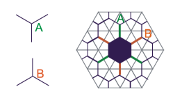
Figure 12: Label of the dual lattice by A and B. All edges going into sinks from $J_{h}$ sides is connected to A vertices and those going into sinks from $-J_{h}$ is connected B vertices

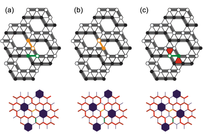
Figure 13: Example of configuration of spins on a maple-lattice and loop-strings on a honeycomb lattice with sinks in (a) UUD-1 stripe state, (b) when flipping a yellow bond from panel (a), and (c) flipping a green bond from panel (a).

In this section, we give proof to support the discussion in Sec.III that the energy values of all UUD/DDU states are independent of $J_{h}$ in the case of $J_{h1}=-J_{h2}=J_{h}$. Notice that all UUD/DDU states in the maple-leaf lattice are mapped one-to-one to a fully packed loop-string configuration on its dual lattice. Then, one only needs to prove in the fully packed loop-string state that the number of loop-bonds on a dual lattice going into a sink crossing the $J_{h}$-edge of the hexagon of the maple-leaf lattice is equal to the number of loop-bonds crossing the $(-J_{h})$-edge. Let us label the vertices on the dual lattice by “A” and “B” as shown in Fig. 12.

In a fully packed loop-string state, the number of bonds connected to A vertices is equal to that to B vertices since the number of bonds connected to each vertex is the same between the two. This means that the number of bonds going into a sink from A vertices and that from B vertices are the same; this is because the bond not going into a sink always connects an A vertice and a B vertice and does not affect the balance between the numbers of bonds connected to A and B. Since all edges going into sinks through $J_{h}$ is connected to A vertices and those going into sinks through $-J_{h}$ is connected B vertices, our statement is proved.

Appendix B Effect of ${\cal H}_{xy}$ on the UUD-1 stripe state

We show in Fig. 13 how the spin configuration of UUD-1 stripe in panel (a) changes by flipping the yellow bond to the other UUD-1 state in panel (b). When flipping the green bond in panel (a) the non-UUD state in panel (c) is realized. The corresponding loop-string configuration on the honeycomb lattice with sink is shown in the lower panels. Notice that the UUD/DDU triangles are not equivalent in their Ising energy unlike the triangular lattice antiferromagnet. This is because the UUD structure does not necessarily optimize the energy of each triangle locally; there are positive and negative $\pm J_{h}$ which can be smaller in amplitude than $J$.

Appendix C Comparison of magnetic susceptibilities of several models

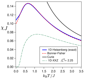
Figure 14: Comparison of magnetic susceptibility of one-dimensional antiferromagnetic Heisenberg model, Bonner-Fisher plot, one-dimensional antiferromagnetic XXZ model for several choices of $J^{1d}_{z}/J^{1d}_{xy}$ with $J^{1d}_{xy}=J$, and Curie plot $J/4k_{\mathrm{B}}T$.

The comparison of magnetic susceptibilities of several models is shown in Fig. 14. The magnetic susceptibility of the one-dimensional Heisenberg model is obtained from exact solution using quantum transfer matrix methodKlümper and Johnston (2000) and its result is numerically evaluated within a negligibly small error. The Bonner-Fisher curveBonner and Fisher (1964) which is first determined by the finite-size scaling to the finite cluster ED results obeys

$$\chi_{\mathrm{BF}}=\frac{0.25+0.14995x+0.30094x^{2}}{k_{\mathrm{B}}T(1+1.9862x+0.68854x^{2}+6.0626x^{3})},$$

with $x=J^{1d}/2k_{\mathrm{B}}T$. One finds that the Bonner-Fisher curve deviates from the exact solution at $k_{B}T/J\lesssim 0.4$. The logarithmic drop of $\chi$ takes place at extremely low temperature below the data obtained, which requires a more accurate numerical integration of Ref.[Klümper and Johnston, 2000]. The Curie plot is given by $\chi_{\mathrm{C}}=1/4k_{\mathrm{B}}T$. The magnetic susceptibility of the one-dimensional XXZ model is obtained for $J^{1d}_{z}/J^{1d}_{xy}=2.25$(the same as in Fig.9) by a size-free calculation using a sine-square deformation combined with the TPQ methodHotta and Asano (2018).

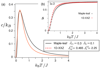
Figure 15: (a) Specific heat per site $c/k_{\rm B}$ calculated using TPQ and sine-square deformation. The parameters of the maple-leaf Heisenberg model and 1D XXZ model are the same as Fig. 9. (b) Entropy density for the data in panel (a).

Appendix D Other physical quantities

The dimensional reduction effect appears in the magnetic properties of the system. To clarify this point, we show in Fig. 15(a) the specific heat per site $c/k_{B}$ of the maple-leaf lattice Heisenberg model with $J_{t1}=0.3$ and $J_{h}=0.1$ which are the same parameters with Fig. 9. Here, we compare it with the result of the 1D XXZ model. For the 1D XXZ model, we used the TPQ combined with a sine-square deformationHotta and Asano (2018) and extracted the center energy bond to evaluate the energy. The specific heat is obtained by the derivative of the energy. The $N=20$ and 24 results agree within the accuracy of ${\cal O}(10^{-3})$ with basically negligible size effect characteristic of the sine-square deformationHotta and Shibata (2012). The horizontal axis is scaled as $J^{1d}_{xy}=0.465$ in the same manner as Fig. 9; the peak positions of the $c/k_{B}$ of two models agree very well, while above the peak temperature, there are extra contributions for the maple leaf lattice.

The difference may come from the nonmagnetic contribution to the specific heat. The nonmagnetic lowest energy excitation of the XXZ model exists below the spin gap, but for the maple-leaf lattice, the lowest energy excitation is the magnetic one. As we saw in Fig. 5(c), the stripe ordering is weakened above the peak temperature, and the other UUD/DDU-1 and non-UUD states may appear. These extra contributions would explain the difference. The entropy obtained by integrating $c/T$ is given in Fig. 15(b) which supports that below the spin gap $\sim 0.5J$ the nonmagnetic contributions appear only for the XXZ model.

Figure 16 shows the magnetization curve of the system, where we plotted the stepwise structure obtained by the exact diagonalization for $N=18$ and 24 clusters and the curve obtained by applying a kernel regression methodNakamura (2020); Harada (2011) to these data. Here, we chose the data below and above the 1/3-plateaus separately. For $J_{t1}=0.3$ we also have 2/3-plateau for $J_{h}=0\sim 1$, which we applied the same treatment. Using the discrete energy levels $e(m)$ from ED as a function of magnetization density $m$, a continuous function $e(m)$ is obtained for each region. Since the value $h=\partial e(m)/\partial m$ at $m=1/6$ differs for those obtained based on the data at $m<1/6$ and $m>1/6$ we find the 1/3-plateau. For $J_{h}/J=0.1$ and $J_{t1}=0.3$ the onset of the curve reminds us of a square-root critical behavior, $m\propto|h-h_{c}|^{1/\delta}$ with $\delta=2$ characteristic of a one dimensional spin gapped systemSakai and Takahashi (1998). However, for $J_{h}/J=1$ it becomes close to $\delta\sim 1$ expected for two-dimensional quantum magnetsSakai and Nakano (2011). These results also support the dimensional reduction of the system observed for small $J_{h}/J$.

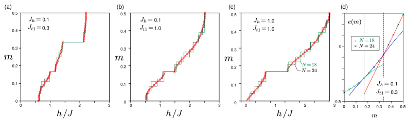
Figure 16: Magnetization curve obtained for (a) $(J_{h},J_{t1})=(0.1,0.3)$, (b)$(0.1,1.0)$ and (c)$(1.0,1.0)$. The stepwise data in solid lines are from the exact diagonalization on $N=18$ and 24 clusters and the data points on curves are obtained using the kernel regression method. Panel (d) shows the energy $e(m)$ of $N=18$ and 24 corresponding to panel (a) as a function of magnetization density $m=\langle s^{z}\rangle/N$, and the three lines are the results of the kernel regression given independently for regions separated by the 1/3 and 2/3 plateaus. We take the mirror for the data below and above the plateaus following Ref.Nakamura, 2020.

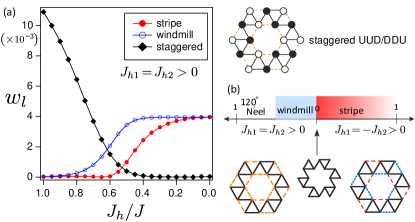
Figure 17: (a) Weights $w_{l}$ for three major contributions for the fully antiferromagnetic $J_{h1}=J_{h2}=J_{h}$ are shown. The staggered state has the antferromagnetic correlation along the hexagon, and appears only for this fully antiferromagnetic case. (b) The overall phase diagram obtained by varying $J_{h1}=\pm J_{h2}$.

Appendix E Antiferromagnetic case $J_{h1}=J_{h2}>0$

We examine the case where all the interactions are antiferromagnetic. Figure 17(a) shows the weight of the ground state wave function $w_{l}$ for $N=18$. The stripe, windmill and staggered type configurations show the major contribution. The parameter range corresponds to Fig. 2(b). The staggered state shown in the right panel is the one not found for $J_{h_{1}}=-J_{h_{2}}$ case, and show the antiferromagnetic correlation around the hexagon. This state and the windmill state are spatially isotropic with a purely two-dimensional character, and the staggered state contribute to the $120^{\circ}$ Néel order reported earlierSchulenburg et al. (2000); Schmalfuß et al. (2002). The overall phase diagram is shown in Fig. 17(b). The stripe and the dimensional reduction are expected for small and mixed $J_{h_{1}}=-J_{h_{2}}$ region.

References

- Villain, J. et al. (1980) Villain, J., Bidaux, R., Carton, J.-P., and Conte, R., J. Phys. France 41, 1263 (1980).
- Henley (1987) C. L. Henley, J. Appl. Phys. 61, 3962 (1987).
- Gvozdikova and Zhitomirsky (2005) M. V. Gvozdikova and M. E. Zhitomirsky, JETP Lett. 81, 236 (2005).
- Ramirez et al. (1999) A. P. Ramirez, A. Hayashi, R. J. Cava, R. Siddharthan, and B. Shastry, Nature 399, 333 (1999).
- Bramwell and M. (2001) S. T. Bramwell and G. M., Science 294, 1495 (2001).
- Heidarian and Damle (2005) D. Heidarian and K. Damle, Phys. Rev. Lett. 95, 127206 (2005).
- Wessel and Troyer (2005) S. Wessel and M. Troyer, Phys. Rev. Lett. 95, 127205 (2005).
- Melko et al. (2005) R. G. Melko, A. Paramekanti, A. A. Burkov, A. Vishwanath, D. N. Sheng, and L. Balents, Phys. Rev. Lett. 95, 127207 (2005).
- Jolicoeur and Le Guillou (1989) T. Jolicoeur and J. C. Le Guillou, Phys. Rev. B 40, 2727 (1989).
- Bernu et al. (1994) B. Bernu, P. Lecheminant, C. Lhuillier, and L. Pierre, Phys. Rev. B 50, 10048 (1994).
- White and Chernyshev (2007) S. R. White and A. L. Chernyshev, Phys. Rev. Lett. 99, 127004 (2007).
- Fazekas and Anderson (1974) P. Fazekas and P. W. Anderson, Philos. Mag. 30, 423 (1974).
- Anderson (1987) P. W. Anderson, Science 235, 1196 (1987).
- Liao et al. (2017) H. J. Liao, Z. Y. Xie, J. Chen, Z. Y. Liu, H. D. Xie, R. Z. Huang, B. Normand, and T. Xiang, Phys. Rev. Lett. 118, 137202 (2017).
- Depenbrock et al. (2012) S. Depenbrock, I. P. McCulloch, and U. Schollwöck, Phys. Rev. Lett. 109, 067201 (2012).
- Yan et al. (2011) S. Yan, D. A. Huse, and S. R. White, Science 332, 1173 (2011).
- Nishimoto et al. (2013) S. Nishimoto, N. Shibata, and C. Hotta, Nature Communications 4, 2287 (2013).
- Arrachea et al. (2004) L. Arrachea, L. Capriotti, and S. Sorella, Phys. Rev. B 69, 224414 (2004).
- Koretsune et al. (2009) T. Koretsune, M. Udagawa, and M. Ogata, Phys. Rev. B 80, 075408 (2009).
- Sebastian et al. (2006) S. E. Sebastian, N. Harrison, C. D. Batista, L. Balicas, M. Jaime, P. A. Sharma, N. Kawashima, and I. R. Fisher, Nature 441, 617 (2006).
- Rösch and Vojta (2007) O. Rösch and M. Vojta, Phys. Rev. B 76, 180401 (2007).
- Granado et al. (2013) E. Granado, J. W. Lynn, R. F. Jardim, and M. S. Torikachvili, Phys. Rev. Lett. 110, 017202 (2013).
- Okuma et al. (2021) R. Okuma, M. Kofu, S. Asai, M. Avdeev, A. Koda, H. Okabe, M. Hiraishi, S. Takeshita, K. M. Kojima, R. Kadono, T. Masuda, K. Nakajima, and Z. Hiroi, Nature Communications 12, 4382 (2021).
- Skoulatos et al. (2017) M. Skoulatos, M. Månsson, C. Fiolka, K. W. Krämer, J. Schefer, J. S. White, and C. Rüegg, Phys. Rev. B 96, 020414 (2017).
- Coldea et al. (2003) R. Coldea, D. A. Tennant, and Z. Tylczynski, Phys. Rev. B 68, 134424 (2003).
- Kohno et al. (2007) M. Kohno, O. A. Starykh, and L. Balents, Nature Physics 3, 790 (2007).
- Hotta and Pollmann (2008) C. Hotta and F. Pollmann, Phys. Rev. Lett. 100, 186404 (2008).
- Fennell et al. (2011) T. Fennell, J. O. Piatek, R. A. Stephenson, G. J. Nilsen, and H. M. Rønnow, Journal of Physics: Condensed Matter 23, 164201 (2011).
- Kampf et al. (2013) A. R. Kampf, S. J. Mills, R. M. Housley, and J. Marty, American Mineralogist 98, 506 (2013).
- Mills et al. (2014) S. Mills, A. R. Kampf, A. Christy, R. Housley, G. Rossman, R. Reynolds, and J. Marty, Mineralogical Magazine 78, 1325 (2014).
- Cave et al. (2006) D. Cave, F. C. Coomer, E. Molinos, H.-H. Klauss, and P. T. Wood, Angew. Chem. 118, 817 (2006).
- Aliev et al. (2012) A. Aliev, M. Huvé, S. Colis, M. Colmont, A. Dinia, and O. Mentré, Angew. Chem. 124, 9527 (2012).
- Haraguchi et al. (2018) Y. Haraguchi, A. Matsuo, K. Kindo, and Z. Hiroi, Phys. Rev. B 98, 064412 (2018).
- Haraguchi et al. (2021) Y. Haraguchi, A. Matsuo, K. Kindo, and Z. Hiroi, “Quantum antiferromagnet bluebellite comprising a maple-leaf lattice made of spin-1/2 cu2+ ions,” (2021), arXiv:2111.09514 [cond-mat.str-el] .
- Schulenburg et al. (2000) J. Schulenburg, J. Richter, and D. Betts, Acta Physica Polonica A 97, 971 (2000).
- Schmalfuß et al. (2002) D. Schmalfuß, P. Tomczak, J. Schulenburg, and J. Richter, Phys. Rev. B 65, 224405 (2002).
- Farnell et al. (2011) D. J. J. Farnell, R. Darradi, R. Schmidt, and J. Richter, Phys. Rev. B 84, 104406 (2011).
- Bonner and Fisher (1964) J. C. Bonner and M. E. Fisher, Phys. Rev. 135, A640 (1964).
- Venkatesh et al. (2020) C. Venkatesh, B. Bandyopadhyay, A. Midya, K. Mahalingam, V. Ganesan, and P. Mandal, Phys. Rev. B 101, 184429 (2020).
- Wannier (1950) G. H. Wannier, Phys. Rev. 79, 357 (1950).
- Lacorre (1987) P. Lacorre, J. Phys. C: Solid State Phys. 20, L775 (1987).
- Pollmann et al. (2014) F. Pollmann, K. Roychowdhury, C. Hotta, and K. Penc, Phys. Rev. B 90, 035118 (2014).
- Jaklič and Prelovšek (1994) J. Jaklič and P. Prelovšek, Phys. Rev. B 49, 5065 (1994).
- Aichhorn et al. (2003) M. Aichhorn, M. Daghofer, H. G. Evertz, and W. von der Linden, Phys. Rev. B 67, 161103 (2003).
- Hams and De Raedt (2000) A. Hams and H. De Raedt, Phys. Rev. E 62, 4365 (2000).
- Sugiura and Shimizu (2012) S. Sugiura and A. Shimizu, Phys. Rev. Lett. 108, 240401 (2012).
- Hotta and Asano (2018) C. Hotta and K. Asano, Phys. Rev. B 98, 140405 (2018).
- Klümper and Johnston (2000) A. Klümper and D. C. Johnston, Phys. Rev. Lett. 84, 4701 (2000).
- Hotta and Shibata (2012) C. Hotta and N. Shibata, Phys. Rev. B 86, 041108 (2012).
- Nakamura (2020) T. Nakamura, Scientific Reports 10, 14201 (2020).
- Harada (2011) K. Harada, Phys. Rev. E 84, 056704 (2011).
- Sakai and Takahashi (1998) T. Sakai and M. Takahashi, Phys. Rev. B 57, R8091 (1998).
- Sakai and Nakano (2011) T. Sakai and H. Nakano, Phys. Rev. B 83, 100405 (2011).