Fourier-domain transfer entropy spectrum

Abstract

We propose the Fourier-domain transfer entropy spectrum, a novel generalization of transfer entropy, as a model-free metric of causality. For arbitrary systems, this approach systematically quantifies the causality among their different system components rather than merely analyze systems as entireties. The generated spectrum offers a rich-information representation of time-varying latent causal relations, efficiently dealing with non-stationary processes and high-dimensional conditions. We demonstrate its validity in the aspects of parameter dependence, statistic significance test, and sensibility. An open-source multi-platform implementation of this metric is developed and computationally applied on neuroscience data sets and diffusively coupled logistic oscillators.

1 Introduction

Measuring causality between systems is critical in numerous scientific disciplines, ranging from physics Pikovsky et al. (2003) to neuroscience Pereda et al. (2005). The challenge of such measurement arises from a widespread situation where only a limited set of time series of systems are given, and the prior knowledge of their coupling relations remains absent. Over last decades, identifying and quantifying causal relations with insufficient information has become one of the frontier problems in physics, mathematics, and statistics Hlaváčková-Schindler et al. (2007). Substantial progress has been accomplished in measuring causality from statistics-theoretical (e.g., Granger causality Granger (1969) and its generalizations Marinazzo et al. (2008); Ancona et al. (2004); Ho et al. (2004); Arnold et al. (2007); Liu et al. (2009); Dhamala et al. (2008)) and information-theoretical (e.g., transfer entropy Schreiber (2000) and its generalizations Staniek and Lehnertz (2008); Lobier et al. (2014); Lungarella et al. (2007); Runge et al. (2012); Wollstadt et al. (2014); Porfiri and Ruiz Marín (2019); Restrepo et al. (2020); Zhang et al. (2019); Silini and Masoller (2021)) perspectives. Although the nature of causality remains controversial Pearl et al. (2000), these two perspectives have been demonstrated to have non-parametric connections in mathematics Diks and Panchenko (2005); Diks and DeGoede (2001) and share equivalent ideas in potential causality detection. Following their ideas, the existence of causality between systems $\mathsf{X}$ and $\mathsf{Y}$ (e.g., $\mathsf{X}$ is the cause of $\mathsf{Y}$) can be interpreted as

$$\mathcal{P}\left(\mathsf{Y}\left(t\right),\mathsf{X}_{\left[t,\beta,\Delta t\right]}\mid\mathsf{Y}_{\left[t,\beta,\Delta t\right]}\right)\neq\mathcal{P}\left(\mathsf{Y}\left(t\right)\mid\mathsf{Y}_{\left[t,\beta,\Delta t\right]}\right)\mathcal{P}\left(\mathsf{X}_{\left[t,\beta,\Delta t\right]}\mid\mathsf{Y}_{\left[t,\beta,\Delta t\right]}\right),$$ (1)

where $\mathcal{P}\left(\cdot\right)$ denotes the probability. We mark $\mathsf{X}_{\left[t,\beta,\Delta t\right]}=\left(\mathsf{X}\left(t-\beta\Delta t\right),\ldots,\mathsf{X}\left(t-\Delta t\right)\right)$ as the history of $\mathsf{X}$ with time lag unit $\Delta t$ and maximum lag number $\beta$, representing the information of system $\mathsf{X}$ during a time interval $\left[t-\beta\Delta t,t-\Delta t\right]$. In general, inequality (1) means that the uncertainty of $\mathsf{Y}$ at moment $t$ given its own historical information (term $\mathsf{Y}_{\left[t,\beta,\Delta t\right]}$) will be regulated if the historical information of $\mathsf{X}$ (term $\mathsf{X}_{\left[t,\beta,\Delta t\right]}$) is added.

Among various causality metrics, transfer entropy Schreiber (2000) features plentiful applications (e.g., in neuroscience Vicente et al. (2011); Victor (2002); Vakorin et al. (2010); Spinney et al. (2017); Ursino et al. (2020) and economics Dimpfl and Peter (2013); Papana et al. (2016); Toriumi and Komura (2018); Camacho et al. (2021); Ji et al. (2018)) because of its robust capacity to capture non-linear causality and intrinsic connections with dynamics theory and information theory Schreiber (2000); Hlaváčková-Schindler et al. (2007). The initial version of transfer entropy can be defined as

$$\mathcal{T}\left(\mathsf{X},\mathsf{Y}\right)=\mathbb{E}_{t\in\left[\tau+1,n\right]}\Big{\{}\mathcal{D}\Big{[}\mathcal{P}\left(\mathsf{Y}\left(t\right),\mathsf{X}_{\left[t,\beta,\Delta t\right]}\mid\mathsf{Y}_{\left[t,\beta,\Delta t\right]}\right)\Big{\|}\mathcal{P}\left(\mathsf{Y}\left(t\right)\mid\mathsf{Y}_{\left[t,\beta,\Delta t\right]}\right)\otimes\mathcal{P}\left(\mathsf{X}_{\left[t,\beta,\Delta t\right]}\mid\mathsf{Y}_{\left[t,\beta,\Delta t\right]}\right)\Big{]}\Big{\}},$$ (2)

actually equivalent to conditional mutual information Cover (1999); Hlaváčková-Schindler et al. (2007). Equality (2) quantifies the regulating effects in inequality (1) in terms of the expectation of the mutual information between $\mathsf{Y}\left(t\right)$ and $\mathsf{X}_{\left[t,\beta,\Delta t\right]}$ given $\mathsf{Y}_{\left[t,\beta,\Delta t\right]}$. While the model-free property of transfer entropy suggests its general applicability, its application in many real situations is still limited by various deficiencies, such as dimensionality curse Runge et al. (2012) and noise sensitivity Smirnov (2013). Although extensive efforts have been devoted to optimizing transfer entropy estimation in real data (e.g., through symbolization Staniek and Lehnertz (2008), phase time-series Lobier et al. (2014), ensemble evaluation Wollstadt et al. (2014), Lempel-Ziv complexity Restrepo et al. (2020), artificial neural networks Zhang et al. (2019), and $k$-nearest-neighbor Kraskov et al. (2004)), several perspectives remain to be improved:

• Previous works primarily analyze systems as entireties, yet it is more ubiquitous that causality only originates from specific system components (e.g., there only exists causality between the low frequency components of $\mathsf{X}$ and $\mathsf{Y}$). Such causality may be veiled if we do not distinguish between different system components;

• Causality is time-varying. Although the initial version of transfer entropy can be calculated accumulatively or in sliding time windows, a more natural and accurate measurement remains absent;

• Probability density estimation, a prerequisite of transfer entropy calculation, may be costly (e.g., critically requires a large sample size) or inaccurate (e.g., in non-stationary systems and high-dimensional spaces). Although some approaches (e.g., ensemble evaluation in cyclo-stationary systems Wollstadt et al. (2014); Gardner et al. (2006) and $k$-nearest-neighbor estimation Kraskov et al. (2004) in high-dimensional spaces) are developed to optimize the estimation, a low-cost transfer entropy generalization born to deal with non-stationary systems is demanded.

In this letter, we discuss the possibility of generalizing transfer entropy into a form that maintains its original advantages and makes progress in aspects of (I-III). To devote to open science, we release a multi-platform code implementation of our metric and demonstrate its validity on multiple data sets in neuroscience and physics.

2 Fourier-domain representation of systems

An arbitrary system $\mathsf{X}$ can be subdivided into a set of components according to different criteria. To maintain the model-free property of transfer entropy measurement, we concentrate on a universal criterion subdividing $\mathsf{X}$ into different frequency components, namely Fourier-domain (frequency-domain) representation. Such a representation features widespread applications in physics Marks II (2009), mathematics Brémaud (2013), neuroscience Bruns (2004), and engineering Rabiner and Gold (1975), partly ensuring the general applicability of our approach.

To avoid the stationary assumption, one can derive the Fourier-domain representation $\mathcal{F}\left(\mathsf{X},t,\omega\right)$ of $\mathsf{X}$ (here $\omega$ denotes frequency) applying wavelet (WT) Rioul and Vetterli (1991) or Hilbert-Huang transform (HHT) Huang (2014) rather than Fourier transform (FT) owing to the limitations of FT for non-stationary processes Kaiser and Hudgins (1994). In general, WT convolves $\mathsf{X}$ with oscillatory kernels of different frequency bands to realize time-frequency localization Rioul and Vetterli (1991) while HHT directly measures the instantaneous frequency of $\mathsf{X}$ Huang (2014). Although WT and HHT support time-frequency analysis irrespective of stationary assumption, they are still not ideal owing to certain limitations and should be selected according to circumstances Folland and Sitaram (1997); Huang (2014). Here we choose WT to conduct our derivations owing to its complete mathematical foundations, yet other frameworks (e.g., HHT and its variant Peng et al. (2005)) can also be applied.

In terms of continuous WT spectrum, the Fourier-domain representation $\mathcal{F}\left(\mathsf{X},t,\omega\right)$ can be obtained through Ogden (1997); Chun-Lin (2010); Coifman et al. (1992)

$$\mathcal{F}\left(\mathsf{X},t,\omega\right) =\mathsf{W}_{\psi}\big{(}\mathsf{X},t,\zeta_{\psi}\left(\omega\right)\big{)}\mathsf{W}_{\psi}^{\heartsuit}\big{(}\mathsf{X},t,\zeta_{\psi}\left(\omega\right)\big{)},$$ (3)

$$\mathsf{W}_{\psi}\left(\mathsf{X},t,s\right) =\frac{1}{\sqrt{s}}\int\psi^{\heartsuit}\left(\frac{\tau-t}{s}\right)\mathsf{X}\left(\tau\right)d\tau,$$ (4)

where $\psi\in L^{2}\left(\mathbb{R}\right)$ denotes a mother wavelet function (e.g., Morlet wavelets) and notion $\heartsuit$ represents conjugate. Notions $s$ and $\tau$ denote the scaling (frequency localization) and the translation (time localization) parameters, respectively. Function $\zeta_{\psi}\left(\cdot\right)$ is the bijective mapping from frequency $\omega$ to scale $s$, varying according to the selection of mother wavelet function $\psi$. Because the approaches in (3-4) have been extensively studied and applied Ogden (1997); Chun-Lin (2010); Coifman et al. (1992), we do not repeat their derivations.

The Fourier-domain representation $\mathcal{F}\left(\mathsf{X},t,\omega\right)$ can function as a time-frequency spectrum $\left(t,\omega\right)$ of system $\mathsf{X}$, where spectrum value denotes the power. In Fig. 1(a), we show the Fourier-domain representation of an open-source near infrared spectroscopy (NIRS, a kind of electromagnetic-spectrum-based brain imaging approach) data set recorded in the superior frontal cortex Cui et al. (2012a, b). Function $\psi$ is set as the Morlet wavelet. Apart from $\mathcal{F}\left(\mathsf{X},t,\omega\right)$ (subject $1$) and $\mathcal{F}\left(\mathsf{Y},t,\omega\right)$ (subject $2$), we also present $\mathcal{F}\left(\mathsf{XY},t,\omega\right)=\mathsf{W}_{\psi}\big{(}\mathsf{X},t,\zeta_{\psi}\left(\omega\right)\big{)}\mathsf{W}_{\psi}^{\heartsuit}\big{(}\mathsf{Y},t,\zeta_{\psi}\left(\omega\right)\big{)}$.

3 Fourier-domain transfer entropy spectrum

Once $\mathcal{F}\left(\mathsf{X},t,\omega\right)$ and $\mathcal{F}\left(\mathsf{Y},t,\omega\right)$ have been given, we turn to quantify the time-varying latent causality between them in terms of transfer entropy. Below, we discuss one possibility of this measurement.

To overcome the deficiency of probability density estimation (see (III)), we transform these spectra by symbolization. Specifically, we generalize the approach in Bandt and Pompe (2002) to implement a two-dimensional symbolization $\widehat{\mathcal{F}}\left(\mathsf{X},t,\omega\right)$ with a time symbolization order $\lambda$ and a frequency symbolization order $\theta$

$$\widehat{\mathcal{F}}\left(\mathsf{X},t,\omega\right) =\big{(}\Lambda_{\mathsf{X}}\left(t,\omega\right),\Theta_{\mathsf{X}}\left(t,\omega\right)\big{)},\;\forall t\geq\lambda,\;\omega\geq\theta,$$ (5)

$$\Lambda_{\mathsf{X}}\left(t,\omega\right) =\sum_{i=1}^{\lambda}\left(\Gamma_{\Lambda}\left(i\right)-1\right)\lambda^{\lambda-i},$$ (6)

$$\Theta_{\mathsf{X}}\left(t,\omega\right) =\sum_{i=1}^{\theta}\left(\Gamma_{\Theta}\left(i\right)-1\right)\theta^{\theta-i},$$ (7)

$$\Gamma_{\Lambda} =\gamma\big{(}\mathcal{F}\left(\mathsf{X},t-\lambda,\omega\right),\ldots,\mathcal{F}\left(\mathsf{X},t,\omega\right)\big{)},$$ (8)

$$\Gamma_{\Theta} =\gamma\big{(}\mathcal{F}\left(\mathsf{X},t,\omega-\theta\right),\ldots,\mathcal{F}\left(\mathsf{X},t,\omega\right)\big{)}.$$ (9)

The above formulas map each $\mathcal{F}\left(\mathsf{X},t,\omega\right)$ to a two-dimensional coordinate $\big{(}\Lambda_{\mathsf{X}}\left(t,\omega\right),\Theta_{\mathsf{X}}\left(t,\omega\right)\big{)}$. The first coordinate component $\Lambda_{\mathsf{X}}\left(t,\omega\right)$ corresponds to the symbolization along the time-line while the second one corresponds to the symbolization along the frequency-line. Both coordinate components are decimal numbers. The symbolization relays on a permutation $\gamma\left(\cdot\right)$ that returns the order of a sequence in ascending sort (e.g., $\gamma\left(1,6,3,10\right)=\left(1,3,2,4\right)$ because $1<3<6<10$). If the order minus one (e.g., $\left(1,3,2,4\right)$ becomes $\left(0,2,1,3\right)$), then it becomes a number in $\lambda$-base (or $\theta$-base) and can be transformed to a decimal number following (6-7). In Fig. 1(b), we show the symbolization results of the NIRS data under two different conditions.

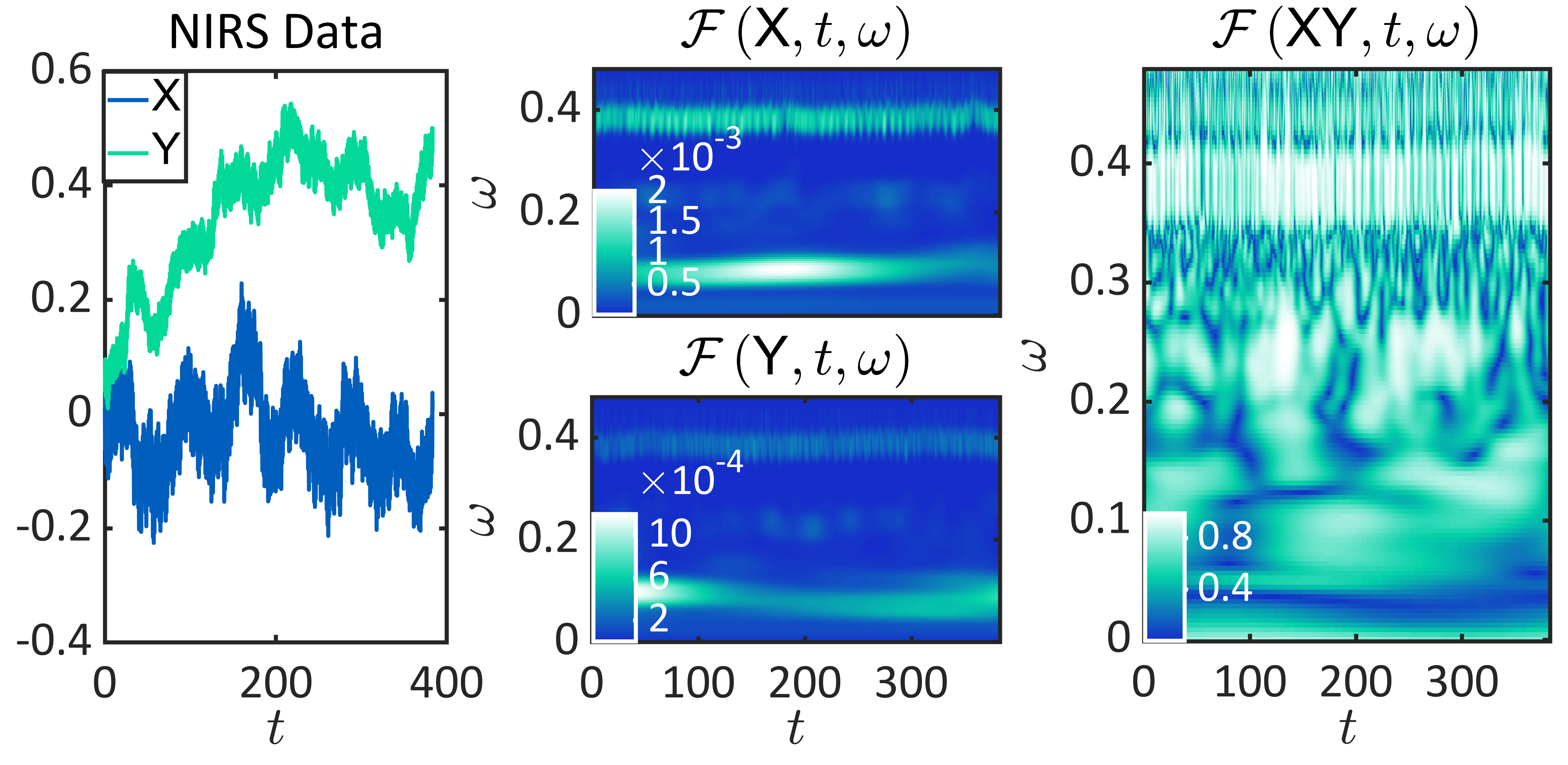
(a)

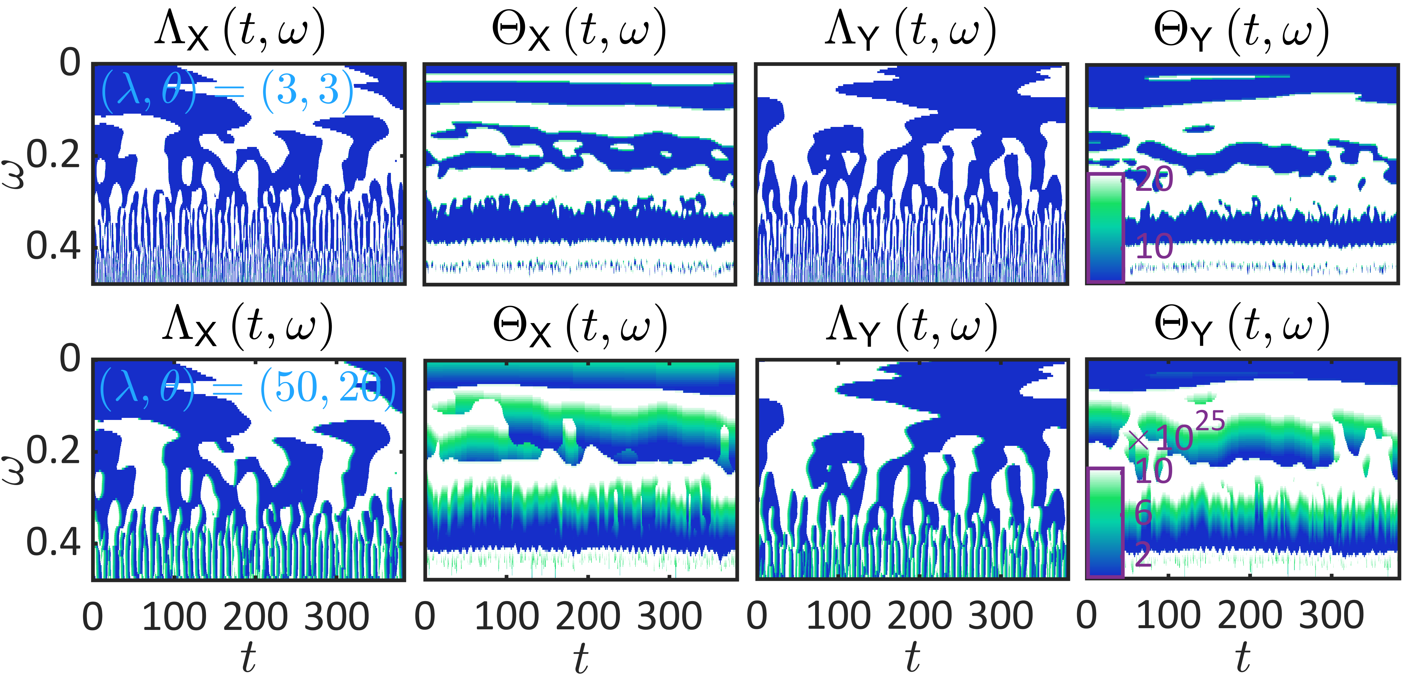
(b)

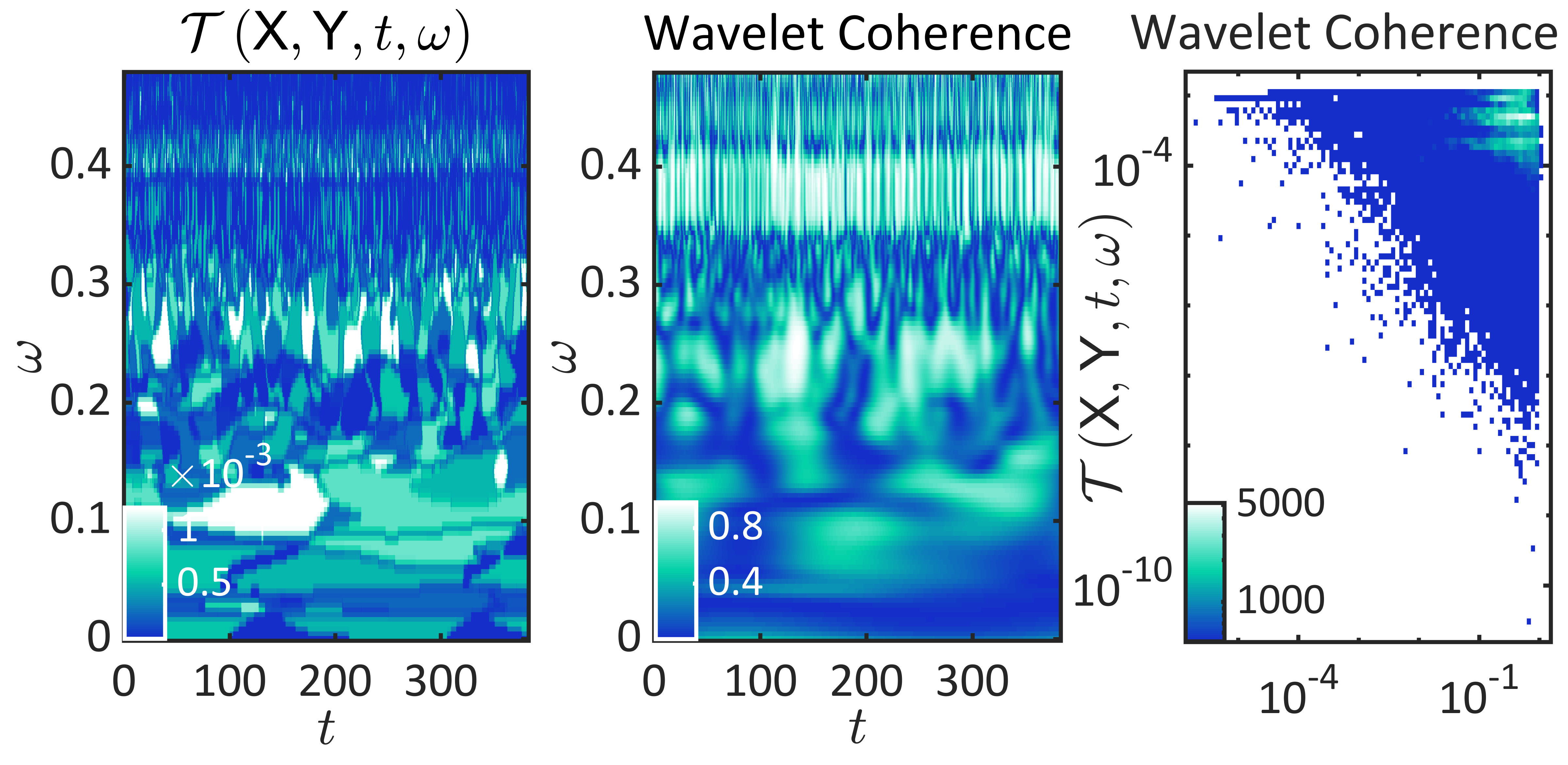
(c)

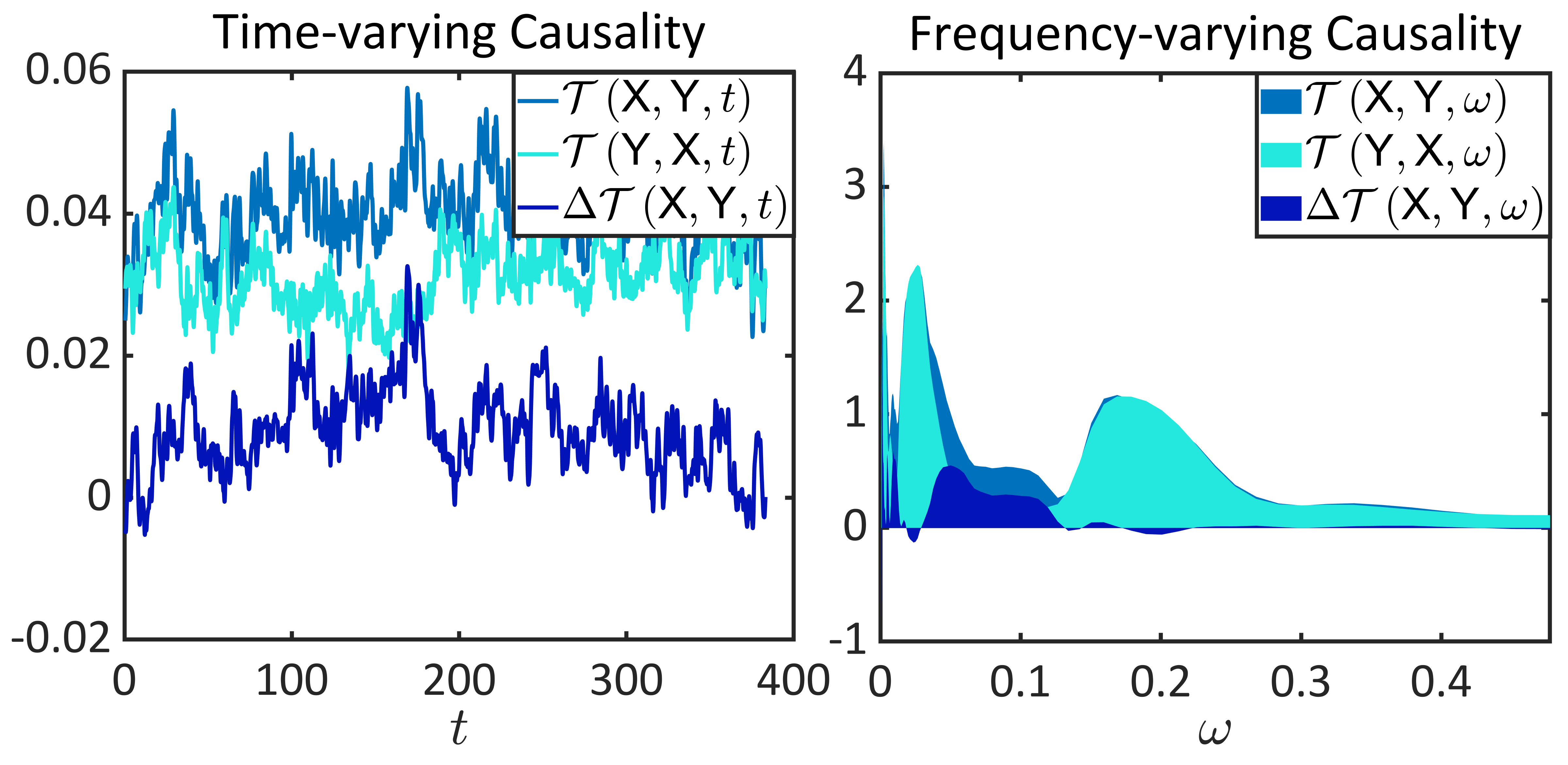
(d)

Figure 1: Fourier-domain transfer entropy spectrum analysis. (a) The Fourier-domain representation of the NIRS data. Please note that the frequency $\omega$ is given as cycles per sample (normalized frequency) in our paper. (b) A coarse-grained symbolization with $\left(\lambda,\theta\right)=\left(3,3\right)$ (upper parallel) and a fine-grained symbolization with $\left(\lambda,\theta\right)=\left(50,20\right)$ (bottom parallel). (c) The Fourier-domain transfer entropy spectrum, the wavelet coherence, and their relation. (d) Time-varying and frequency-varying transfer entropy as well as directional information transfer.

The symbolization benefits to our research by embedding $\mathcal{F}\left(\mathsf{X},t,\omega\right)$, a space with large cardinal number (there are a mass of possibilities of the spectrum value of $\mathcal{F}\left(\mathsf{X},t,\omega\right)$ because the power in (3) is a continuous variable), to a space with much smaller cardinal number ($\widehat{\mathcal{F}}\left(\mathsf{X},t,\omega\right)$ is a discrete space whose cardinal number is no more than $\lambda!$) Bandt and Pompe (2002). It functions as a coarse-graining approach to control noises and supports a more adequate sampling of the historical information (e.g., $\mathsf{X}_{\left[t,\beta,\Delta t\right]}$ in (2)) during probability density estimation (because the variable becomes discrete and its variability is reduced) Porfiri and Ruiz Marín (2019). These benefits should be emphasized especially when $\mathsf{X}$ is non-stationary and a repetitive sampling is not infeasible. In sum, the symbolization in (5-9) can, to a certain extent, alleviate deficiency (III). Parameters $\lambda$ and $\theta$ control the granularity of coarse-graining (e.g., see Fig. 1(b)). They should not be too large. Otherwise, the symbolization is too fine-grained and unnecessary Xie et al. (2019).

After symbolization, the Fourier-domain transfer entropy spectrum can be defined as (10), in which we adopt the notions of (1) to define an abbreviative representation $\widehat{\mathcal{F}}\left(\mathsf{X}_{\left[t,\beta,\Delta t\right]},\omega\right)=\left(\widehat{\mathcal{F}}\left(\mathsf{X},t-\beta\Delta t,\omega\right),\ldots,\widehat{\mathcal{F}}\left(\mathsf{X},t,\omega\right)\right)$. Although formula (10) is consistent with (2), it does not average or sum transfer entropy across time and frequency for a single value. Instead, the transfer entropy in (10) becomes a function of time and frequency, partly overcoming deficiencies (I-II). Note that $\mathcal{T}\left(\mathsf{X},\mathsf{Y},t,\omega\right)$ in (10) can be either positive or negative, respectively corresponding to the case where the added information of $\widehat{\mathcal{F}}\left(\mathsf{X}_{\left[t,\beta,\Delta t\right]},\omega\right)$ reduces or increases the uncertainty of $\widehat{\mathcal{F}}\left(\mathsf{Y},t,\omega\right)$ given $\widehat{\mathcal{F}}\left(\mathsf{Y}_{\left[t,\beta,\Delta t\right]},\omega\right)$ (there is no limitation of the directionality of regulating effects in (1)). To keep consistency with the Granger causality that identifies potential causes through uncertainty (error) reduction Granger (1969), we refer to $\widehat{\mathcal{F}}\left(\mathsf{X}_{\left[t,\beta,\Delta t\right]},\omega\right)$ as a cause of $\widehat{\mathcal{F}}\left(\mathsf{Y},t,\omega\right)$ when $\widehat{\mathcal{F}}\left(\mathsf{X}_{\left[t,\beta,\Delta t\right]},\omega\right)$ is positive. A negative $\widehat{\mathcal{F}}\left(\mathsf{X}_{\left[t,\beta,\Delta t\right]},\omega\right)$ corresponds to a decoupling effect on $\widehat{\mathcal{F}}\left(\mathsf{Y},t,\omega\right)$ and $\widehat{\mathcal{F}}\left(\mathsf{X}_{\left[t,\beta,\Delta t\right]},\omega\right)$ provided by $\widehat{\mathcal{F}}\left(\mathsf{X}_{\left[t,\beta,\Delta t\right]},\omega\right)$.

$$\mathcal{T}\left(\mathsf{X},\mathsf{Y},t,\omega\right)= \mathcal{P}\left(\widehat{\mathcal{F}}\left(\mathsf{Y},t,\omega\right),\widehat{\mathcal{F}}\left(\mathsf{X}_{\left[t,\beta,\Delta t\right]},\omega\right),\widehat{\mathcal{F}}\left(\mathsf{Y}_{\left[t,\beta,\Delta t\right]},\omega\right)\right)$$

$$\log\frac{\mathcal{P}\left(\widehat{\mathcal{F}}\left(\mathsf{Y},t,\omega\right),\widehat{\mathcal{F}}\left(\mathsf{X}_{\left[t,\beta,\Delta t\right]},\omega\right)\mid\widehat{\mathcal{F}}\left(\mathsf{Y}_{\left[t,\beta,\Delta t\right]},\omega\right)\right)}{\mathcal{P}\left(\widehat{\mathcal{F}}\left(\mathsf{Y},t,\omega\right)\mid\widehat{\mathcal{F}}\left(\mathsf{Y}_{\left[t,\beta,\Delta t\right]},\omega\right)\right)\mathcal{P}\left(\widehat{\mathcal{F}}\left(\mathsf{X}_{\left[t,\beta,\Delta t\right]},\omega\right)\mid\widehat{\mathcal{F}}\left(\mathsf{Y}_{\left[t,\beta,\Delta t\right]},\omega\right)\right)}.$$ (10)

In Fig. 1(c), we show the Fourier-domain transfer entropy spectrum of the NIRS data. The symbolization is implemented under a relatively coarse-grained condition $\left(\lambda,\theta\right)=\left(3,3\right)$. Each $\mathcal{T}\left(\mathsf{X},\mathsf{Y},t,\omega\right)$ is measured with $\beta=5$. For convenience, we set each negative $\mathcal{T}\left(\mathsf{X},\mathsf{Y},t,\omega\right)$ as $0$ (this setting can be excluded when the decoupling effects are of interests). In our results, we can see relatively strong and oscillating causality between $\mathsf{X}$ and $\mathsf{Y}$ around $\omega\sim 0.1$, $\omega\sim 0.25$, and $\omega\sim 0.4$. The causality in other frequency regions is relatively weak. We also compare $\mathcal{T}\left(\mathsf{X},\mathsf{Y},t,\omega\right)$ with the well-known wavelet coherence spectrum Torrence and Compo (1998), which quantifies the time-varying and linear coherence between $\mathsf{X}$ and $\mathsf{Y}$. Consistent with the common knowledge, the causality measured by $\mathcal{T}\left(\mathsf{X},\mathsf{Y},t,\omega\right)$ can not be trivially simplified as linear coherence because these two metrics have no clear accordant pattern.

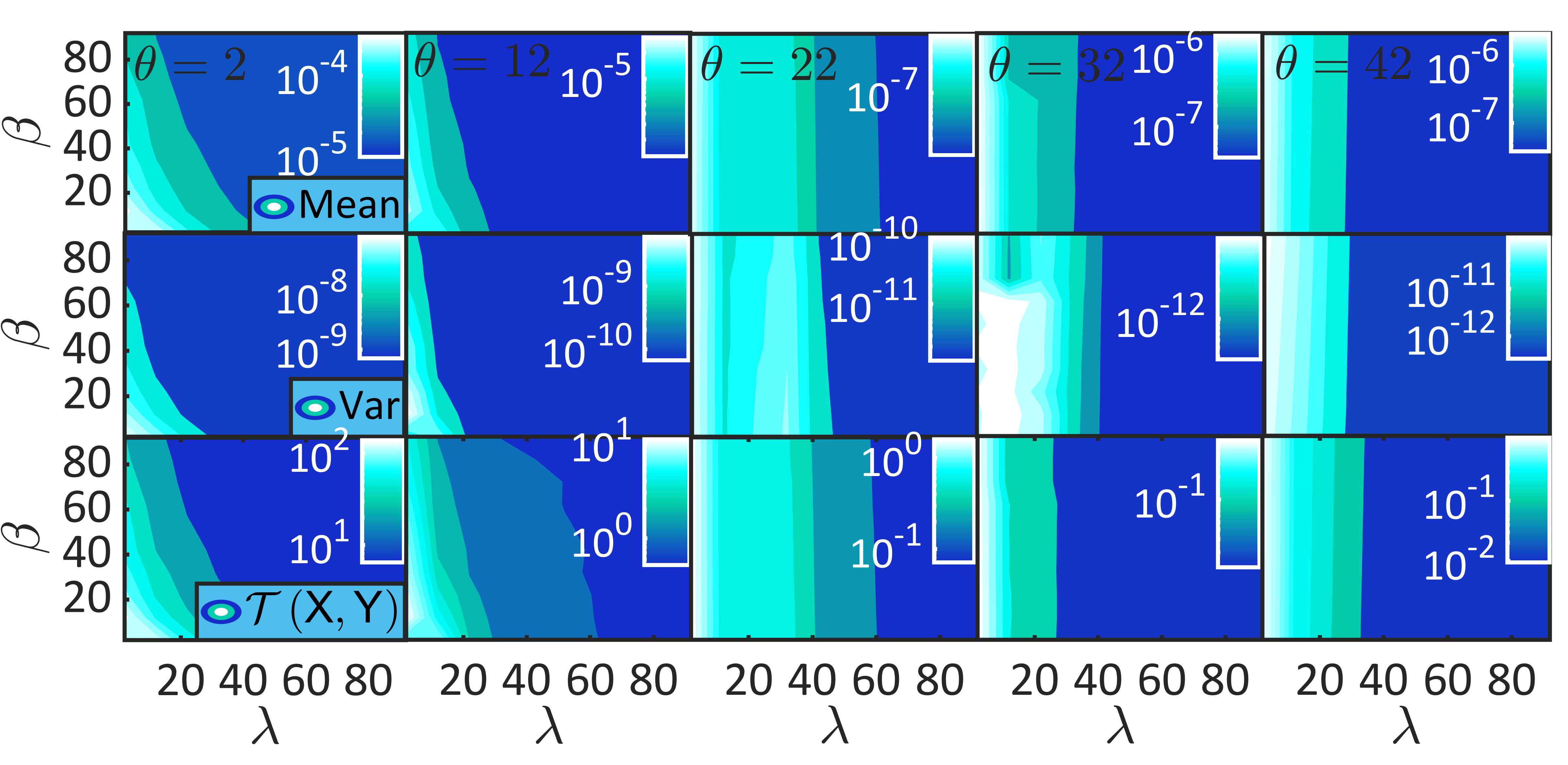
(a)

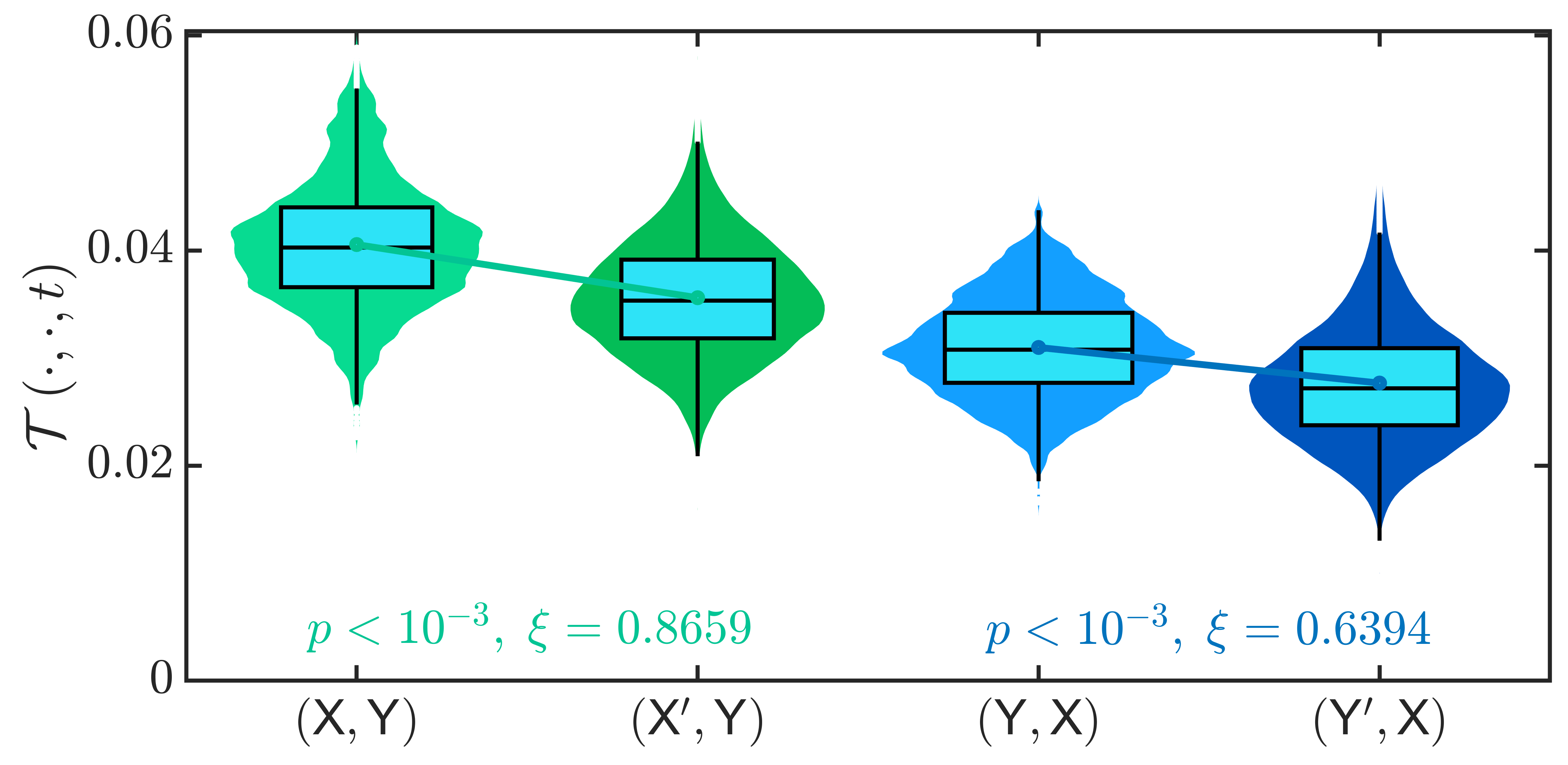
(b)

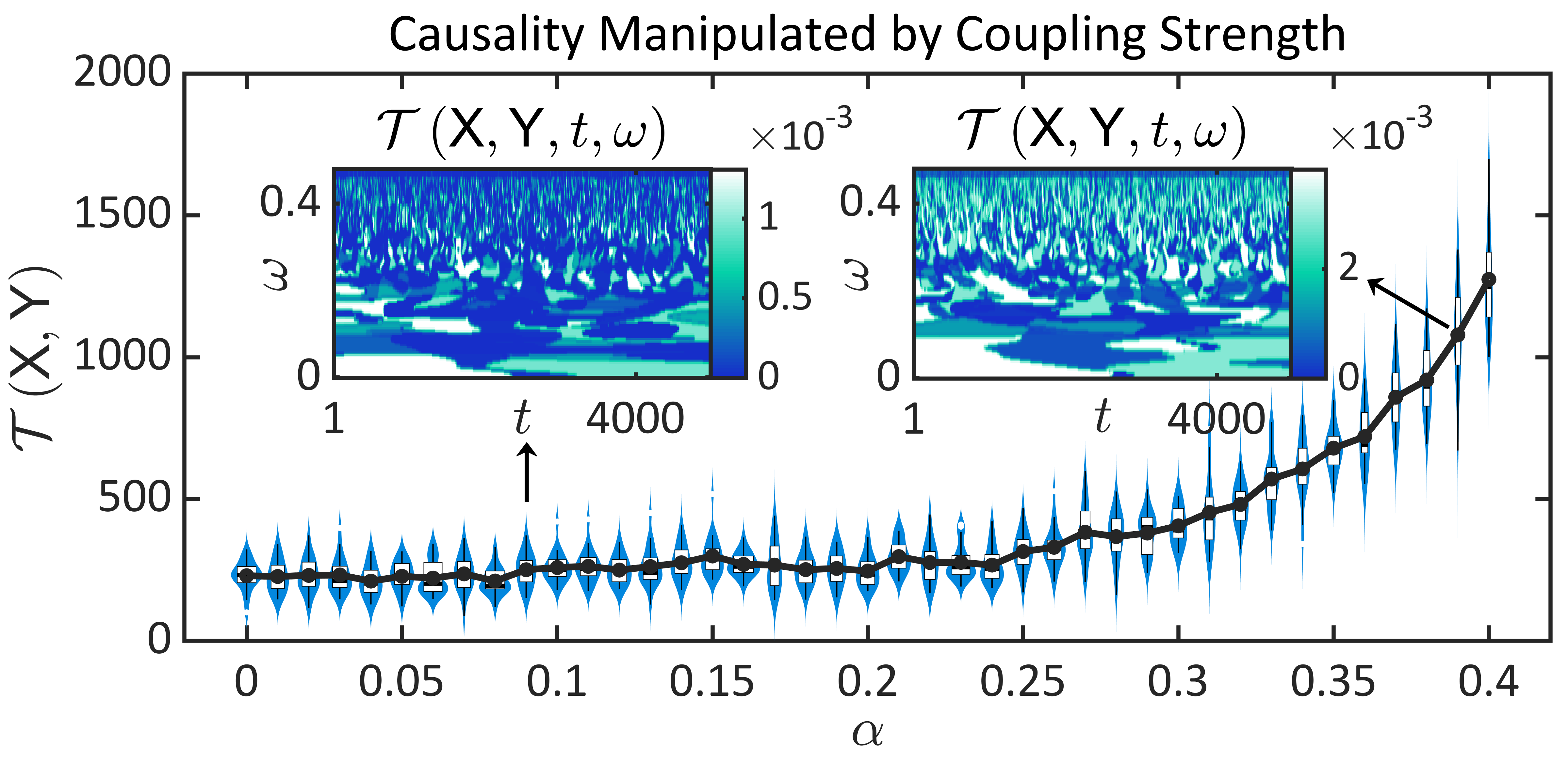
(c)

(d)

Figure 2: Validity analysis of the Fourier-domain transfer entropy spectrum. (a) The dependence of parameter selections. (b) Statistic significance analysis of the Fourier-domain transfer entropy spectrum in Fig. 1(c)-1(d). (c-d) The Fourier-domain transfer entropy spectrum and its effect size is manipulated by the coupling strength $\alpha$.

Meanwhile, we can sum $\mathcal{T}\left(\mathsf{X},\mathsf{Y},t,\omega\right)$ over frequency at each moment (see (11)), over time at each frequency (see (12)), or over both time and frequency (see (13)).

$$\mathcal{T}\left(\mathsf{X},\mathsf{Y},t\right) =\sum_{\omega}\mathcal{T}\left(\mathsf{X},\mathsf{Y},t,\omega\right),\;\forall t,$$ (11)

$$\mathcal{T}\left(\mathsf{X},\mathsf{Y},\omega\right) =\sum_{t}\mathcal{T}\left(\mathsf{X},\mathsf{Y},t,\omega\right),\;\forall\omega,$$ (12)

$$\mathcal{T}\left(\mathsf{X},\mathsf{Y}\right) =\sum_{t,\omega}\mathcal{T}\left(\mathsf{X},\mathsf{Y},t,\omega\right).$$ (13)

Formulas (11-13) denote the varying Fourier-domain transfer entropy across time, frequency, and all possibilities, respectively. Note that $\mathcal{T}\left(\mathsf{X},\mathsf{Y}\right)$ is always non-negative. Combining (11-13) with the asymmetry property of transfer entropy, we define

$$\Delta\mathcal{T}\left(\mathsf{X},\mathsf{Y},t\right) =\mathcal{T}\left(\mathsf{X},\mathsf{Y},t\right)-\mathcal{T}\left(\mathsf{Y},\mathsf{X},t\right),\;\forall t,$$ (14)

$$\Delta\mathcal{T}\left(\mathsf{X},\mathsf{Y},\omega\right) =\mathcal{T}\left(\mathsf{X},\mathsf{Y},\omega\right)-\mathcal{T}\left(\mathsf{Y},\mathsf{X},\omega\right),\;\forall\omega,$$ (15)

$$\Delta\mathcal{T}\left(\mathsf{X},\mathsf{Y}\right) =\mathcal{T}\left(\mathsf{X},\mathsf{Y}\right)-\mathcal{T}\left(\mathsf{Y},\mathsf{X}\right)$$ (16)

to quantify the directional information transfer between $\mathsf{X}$ and $\mathsf{Y}$. In Fig. 1(d), we illustrate these quantities based on the results in Fig. 1(c). A stronger information transfer from $\mathsf{X}$ to $\mathsf{Y}$ can be observed in both time- and frequency-line, surpassing the transfer from $\mathsf{Y}$ to $\mathsf{X}$. Such a directional transfer is significant when $\omega\sim 0.1$.

4 Validity of Fourier-domain transfer entropy spectrum

After proposing the Fourier-domain transfer entropy spectrum, we turn to analyze its validity.

A valid causality metric is demanded to have clear dependence relations with all involved parameters. Although the Fourier-domain transfer entropy spectrum is a model-free metric and has no pre-assumption on system properties, the symbolization and the transfer entropy definition itself still introduce three parameters: $\lambda$, $\theta$, and $\beta$. Serving as coarse-graining parameters, $\lambda$ and $\theta$ determine the granularity of symbolization. Sufficiently large quantities of $\lambda$ and $\theta$ may not only make symbolization meaningless Xie et al. (2019) but also cause obstacles in probability density estimation (because the variability of variables increase). An in-exhaustive sampling frequently underestimates specific parts of the probability density, especially in high-dimensional spaces. Therefore, we speculate that $\mathcal{T}\left(\mathsf{X},\mathsf{Y},t,\omega\right)$ may be underestimated when $\lambda$ and $\theta$ become too large. In Fig. 2(a), we calculate $\mathcal{T}\left(\mathsf{X},\mathsf{Y},t,\omega\right)$ in the NIRS data with different parameters. For convenience, we set each negative $\mathcal{T}\left(\mathsf{X},\mathsf{Y},t,\omega\right)$ as $0$. Consistent with our inference, quantities $\mathbb{E}_{t,\omega}\mathcal{T}\left(\mathsf{X},\mathsf{Y},t,\omega\right)$ (expectation), $\operatorname*{Var}_{t,\omega}\mathcal{T}\left(\mathsf{X},\mathsf{Y},t,\omega\right)$ (variance), and $\mathcal{T}\left(\mathsf{X},\mathsf{Y}\right)$ approximate to $0$ as $\lambda$ and $\theta$ increase. Similar effects can be observed on the lag parameter $\beta$ but become much more slight. In sum, the Fourier-domain transfer entropy spectrum is expected to be implemented with relatively small $\lambda$ and $\theta$. The selection of $\beta$ is less limited and can be carried out according to different demands.

Moreover, a valid causality metric should be equipped with a statistic significance test. Information-theoretical metrics, including our Fourier-domain transfer entropy spectrum, frequently involve biases in finite data sets Panzeri et al. (2007). Therefore, the absolute value of $\mathcal{T}\left(\mathsf{X},\mathsf{Y},t,\omega\right)$ only has limited meaning until being statistically tested. Combining the time-shifting surrogates Andrzejak et al. (2006); Wagner et al. (2010); Martini et al. (2011) with the permutation test Phipson and Smyth (2010); Maris and Oostenveld (2007), we design the significance test as following: (1) Generate a set of surrogates $\{\mathsf{X}^{\prime}_{\delta}|\mathsf{X}^{\prime}_{\delta}\left(t\right)=\mathsf{X}\left(t+\delta\right),\;\delta\in\mathbb{N}^{+}\}$ and calculate $\{\mathcal{T}\left(\mathsf{X}^{\prime}_{\delta},\mathsf{Y},t\right)\}_{t}$ for each surrogate $\mathsf{X}^{\prime}_{\delta}$; (2) Implement permutation test for the difference in mean value between $\{\mathcal{T}\left(\mathsf{X},\mathsf{Y},t\right)\}_{t}$ and $\bigcup_{\delta}\{\mathcal{T}\left(\mathsf{X}^{\prime}_{\delta},\mathsf{Y},t\right)\}_{t}$ to calculate the statistic significance $p$ and the effect size $\xi$. A similar idea can be seen in Lindner et al. (2011). In practice, a weakest condition with $p\leq 10^{-2}$ and $\xi\geq 0.2$ (in the comparison of mean values, $\xi\sim 0.2$, $\xi\sim 0.5$, and $\xi\sim 0.8$ correspond to small, medium, and high effect sizes, respectively) should be satisfied if the Fourier-domain transfer entropy spectrum is statistically significant. In Fig. 2(b), we test the results in Fig. 1(c)-1(d), where $50$ surrogates are generated by randomizing $\delta\in\left[3,100\right]$. The generated $\bigcup_{\delta}\{\mathcal{T}\left(\mathsf{X}^{\prime}_{\delta},\mathsf{Y},t\right)\}_{t}$ features a large sample size of $191350$, supporting a robust statistic test. We implement a large scale permutation test with $5000$ permutations, demonstrating the statistic significance of $\mathcal{T}\left(\mathsf{X},\mathsf{Y},t\right)$ and $\mathcal{T}\left(\mathsf{Y},\mathsf{X},t\right)$ with ideal effect sizes. Meanwhile, the effect size on $\mathcal{T}\left(\mathsf{Y},\mathsf{X},t\right)$ is smaller than that on $\mathcal{T}\left(\mathsf{X},\mathsf{Y},t\right)$, corroborating our observations in Fig. 1(d) about the directional information transfer in the NIRS data.

Finally, a valid causality metric is expected to be sensitive to the changes of coupling strength between $\mathsf{X}$ and $\mathsf{Y}$. In other words, $\mathcal{T}\left(\mathsf{X},\mathsf{Y},t,\omega\right)$ should be regulated as consequences if we manipulate the coupling strength. To realize the manipulation, we consider two diffusively coupled logistic oscillators $\mathsf{X}\rightarrow\mathsf{Y}$ in Fig. 2(c)-2(d). Notion $\rightarrow$ denotes the direction of coupling. Oscillators $\mathsf{X}$ and $\mathsf{Y}$ are defined with a bifurcation parameter $\mu=4$, and their coupling strength is denoted by $\alpha$. For more mathematical details, we refer to Lloyd (1995). We manipulate the coupling strength $\alpha$ from $0$ to $0.4$ and apply an open-source algorithm Valencio and Baptista (2018) to generate the time series of $\mathsf{X}$ and $\mathsf{Y}$ under each $\alpha$ condition. The generation is repeated $50$ times in each case, corresponding to different random initial values. For each pair of time series, we calculate the Fourier-domain transfer entropy spectrum with $\lambda=\theta=3$ and $\beta=1$. Meanwhile, $5$ surrogates are generated by randomizing $\delta\in\left[3,100\right]$, leading to a large sample size $24985$ in the statistic significance test. The number of permutations is set as $5000$. In Fig. 2(c)-2(d), we demonstrate that the Fourier-domain transfer entropy spectrum and its effect sizes (with $p<10^{-2}$) increase with the coupling strength $\alpha$. In other words, the quantified latent causality increases as a consequence of coupling strength enhancement.

5 Conclusion

We present the Fourier-domain transfer entropy spectrum, a model-free metric of causality, to extract the time-varying latent causality among different system components of an arbitrary pair of systems in the Fourier-domain. Built on the wavelet transform and symbolization, our approach can partly alleviate deficiencies (I-III), generally applicable in various non-stationary or high-dimensional processes (e.g., neuroscience data). We have demonstrated the validity of our approach in the aspects of parameter dependence, statistic significance test, and sensibility. An open-source release of our algorithm can be seen in Tian et al. (2021).

6 Acknowledgements

This project is supported by the Artificial and General Intelligence Research Program of Guo Qiang Research Institute at Tsinghua University (2020GQG1017) as well as the Tsinghua University Initiative Scientific Research Program. Correspondence of this research should be addressed to Y.Y.W, Z.Y.Z, and P.S.

References

- Pikovsky et al. [2003] Arkady Pikovsky, Jurgen Kurths, Michael Rosenblum, and Jürgen Kurths. Synchronization: a universal concept in nonlinear sciences. Number 12. Cambridge university press, 2003.
- Pereda et al. [2005] Ernesto Pereda, Rodrigo Quian Quiroga, and Joydeep Bhattacharya. Nonlinear multivariate analysis of neurophysiological signals. Progress in neurobiology, 77(1-2):1–37, 2005.
- Hlaváčková-Schindler et al. [2007] Katerina Hlaváčková-Schindler, Milan Paluš, Martin Vejmelka, and Joydeep Bhattacharya. Causality detection based on information-theoretic approaches in time series analysis. Physics Reports, 441(1):1–46, 2007.
- Granger [1969] Clive WJ Granger. Investigating causal relations by econometric models and cross-spectral methods. Econometrica: journal of the Econometric Society, pages 424–438, 1969.
- Marinazzo et al. [2008] Daniele Marinazzo, Mario Pellicoro, and Sebastiano Stramaglia. Kernel method for nonlinear granger causality. Physical review letters, 100(14):144103, 2008.
- Ancona et al. [2004] Nicola Ancona, Daniele Marinazzo, and Sebastiano Stramaglia. Radial basis function approach to nonlinear granger causality of time series. Physical Review E, 70(5):056221, 2004.
- Ho et al. [2004] Ming-Chung Ho, Yao-Chen Hung, and I-Min Jiang. Phase synchronization in inhomogeneous globally coupled map lattices. Physics Letters A, 324(5-6):450–457, 2004.
- Arnold et al. [2007] Andrew Arnold, Yan Liu, and Naoki Abe. Temporal causal modeling with graphical granger methods. In Proceedings of the 13th ACM SIGKDD international conference on Knowledge discovery and data mining, pages 66–75, 2007.
- Liu et al. [2009] Han Liu, John Lafferty, and Larry Wasserman. The nonparanormal: Semiparametric estimation of high dimensional undirected graphs. Journal of Machine Learning Research, 10(10), 2009.
- Dhamala et al. [2008] Mukeshwar Dhamala, Govindan Rangarajan, and Mingzhou Ding. Estimating granger causality from fourier and wavelet transforms of time series data. Physical review letters, 100(1):018701, 2008.
- Schreiber [2000] Thomas Schreiber. Measuring information transfer. Physical review letters, 85(2):461, 2000.
- Staniek and Lehnertz [2008] Matthäus Staniek and Klaus Lehnertz. Symbolic transfer entropy. Physical review letters, 100(15):158101, 2008.
- Lobier et al. [2014] Muriel Lobier, Felix Siebenhühner, Satu Palva, and J Matias Palva. Phase transfer entropy: a novel phase-based measure for directed connectivity in networks coupled by oscillatory interactions. Neuroimage, 85:853–872, 2014.
- Lungarella et al. [2007] Max Lungarella, Alex Pitti, and Yasuo Kuniyoshi. Information transfer at multiple scales. Physical Review E, 76(5):056117, 2007.
- Runge et al. [2012] Jakob Runge, Jobst Heitzig, Vladimir Petoukhov, and Jürgen Kurths. Escaping the curse of dimensionality in estimating multivariate transfer entropy. Physical review letters, 108(25):258701, 2012.
- Wollstadt et al. [2014] Patricia Wollstadt, Mario Martínez-Zarzuela, Raul Vicente, Francisco J Díaz-Pernas, and Michael Wibral. Efficient transfer entropy analysis of non-stationary neural time series. PloS one, 9(7):e102833, 2014.
- Porfiri and Ruiz Marín [2019] Maurizio Porfiri and Manuel Ruiz Marín. Transfer entropy on symbolic recurrences. Chaos: An Interdisciplinary Journal of Nonlinear Science, 29(6):063123, 2019.
- Restrepo et al. [2020] Juan F Restrepo, Diego M Mateos, and Gastón Schlotthauer. Transfer entropy rate through lempel-ziv complexity. Physical Review E, 101(5):052117, 2020.
- Zhang et al. [2019] Jingjing Zhang, Osvaldo Simeone, Zoran Cvetkovic, Eugenio Abela, and Mark Richardson. Itene: Intrinsic transfer entropy neural estimator. arXiv preprint arXiv:1912.07277, 2019.
- Silini and Masoller [2021] Riccardo Silini and Cristina Masoller. Fast and effective pseudo transfer entropy for bivariate data-driven causal inference. Scientific Reports, 11(1):1–13, 2021.
- Pearl et al. [2000] Judea Pearl et al. Models, reasoning and inference. Cambridge, UK: CambridgeUniversityPress, 19, 2000.
- Diks and Panchenko [2005] Cees Diks and Valentyn Panchenko. A note on the hiemstra-jones test for granger non-causality. Studies in nonlinear dynamics & econometrics, 9(2), 2005.
- Diks and DeGoede [2001] Cees Diks and Jacob DeGoede. A general nonparametric bootstrap test for granger causality. Global analysis of dynamical systems, pages 391–403, 2001.
- Vicente et al. [2011] Raul Vicente, Michael Wibral, Michael Lindner, and Gordon Pipa. Transfer entropy—a model-free measure of effective connectivity for the neurosciences. Journal of computational neuroscience, 30(1):45–67, 2011.
- Victor [2002] Jonathan D Victor. Binless strategies for estimation of information from neural data. Physical Review E, 66(5):051903, 2002.
- Vakorin et al. [2010] Vasily A Vakorin, Natasa Kovacevic, and Anthony R McIntosh. Exploring transient transfer entropy based on a group-wise ica decomposition of eeg data. Neuroimage, 49(2):1593–1600, 2010.
- Spinney et al. [2017] Richard E Spinney, Mikhail Prokopenko, and Joseph T Lizier. Transfer entropy in continuous time, with applications to jump and neural spiking processes. Physical Review E, 95(3):032319, 2017.
- Ursino et al. [2020] Mauro Ursino, Giulia Ricci, and Elisa Magosso. Transfer entropy as a measure of brain connectivity: a critical analysis with the help of neural mass models. Frontiers in computational neuroscience, 14:45, 2020.
- Dimpfl and Peter [2013] Thomas Dimpfl and Franziska Julia Peter. Using transfer entropy to measure information flows between financial markets. Studies in Nonlinear Dynamics and Econometrics, 17(1):85–102, 2013.
- Papana et al. [2016] Angeliki Papana, Catherine Kyrtsou, Dimitris Kugiumtzis, and Cees Diks. Detecting causality in non-stationary time series using partial symbolic transfer entropy: Evidence in financial data. Computational economics, 47(3):341–365, 2016.
- Toriumi and Komura [2018] Fujio Toriumi and Kazuki Komura. Investment index construction from information propagation based on transfer entropy. Computational Economics, 51(1):159–172, 2018.
- Camacho et al. [2021] Maximo Camacho, Andres Romeu, and Manuel Ruiz-Marin. Symbolic transfer entropy test for causality in longitudinal data. Economic Modelling, 94:649–661, 2021.
- Ji et al. [2018] Qiang Ji, Hardik Marfatia, and Rangan Gupta. Information spillover across international real estate investment trusts: Evidence from an entropy-based network analysis. The North American Journal of Economics and Finance, 46:103–113, 2018.
- Cover [1999] Thomas M Cover. Elements of information theory. John Wiley & Sons, 1999.
- Smirnov [2013] Dmitry A Smirnov. Spurious causalities with transfer entropy. Physical Review E, 87(4):042917, 2013.
- Kraskov et al. [2004] Alexander Kraskov, Harald Stögbauer, and Peter Grassberger. Estimating mutual information. Physical review E, 69(6):066138, 2004.
- Gardner et al. [2006] William A Gardner, Antonio Napolitano, and Luigi Paura. Cyclostationarity: Half a century of research. Signal processing, 86(4):639–697, 2006.
- Marks II [2009] Robert J Marks II. Handbook of Fourier analysis & its applications. Oxford University Press, 2009.
- Brémaud [2013] Pierre Brémaud. Mathematical principles of signal processing: Fourier and wavelet analysis. Springer Science & Business Media, 2013.
- Bruns [2004] Andreas Bruns. Fourier-, hilbert-and wavelet-based signal analysis: are they really different approaches? Journal of neuroscience methods, 137(2):321–332, 2004.
- Rabiner and Gold [1975] Lawrence R Rabiner and Bernard Gold. Theory and application of digital signal processing. Englewood Cliffs: Prentice-Hall, 1975.
- Rioul and Vetterli [1991] Olivier Rioul and Martin Vetterli. Wavelets and signal processing. IEEE signal processing magazine, 8(4):14–38, 1991.
- Huang [2014] Norden Eh Huang. Hilbert-Huang transform and its applications, volume 16. World Scientific, 2014.
- Kaiser and Hudgins [1994] Gerald Kaiser and Lonnie H Hudgins. A friendly guide to wavelets, volume 300. Springer, 1994.
- Folland and Sitaram [1997] Gerald B Folland and Alladi Sitaram. The uncertainty principle: a mathematical survey. Journal of Fourier analysis and applications, 3(3):207–238, 1997.
- Peng et al. [2005] ZK Peng, W Tse Peter, and FL Chu. An improved hilbert–huang transform and its application in vibration signal analysis. Journal of sound and vibration, 286(1-2):187–205, 2005.
- Ogden [1997] R Todd Ogden. Essential wavelets for statistical applications and data analysis. Springer, 1997.
- Chun-Lin [2010] Liu Chun-Lin. A tutorial of the wavelet transform. NTUEE, Taiwan, 2010.
- Coifman et al. [1992] Ronald R Coifman, Yves Meyer, and Victor Wickerhauser. Wavelet analysis and signal processing. In In Wavelets and their applications. Citeseer, 1992.
- Cui et al. [2012a] Xu Cui, Daniel M Bryant, and Allan L Reiss. Nirs-based hyperscanning reveals increased interpersonal coherence in superior frontal cortex during cooperation. Neuroimage, 59(3):2430–2437, 2012a.
- Cui et al. [2012b] Xu Cui, Daniel M Bryant, and Allan L Reiss. The nirs data in a built-in directory of matlab, 2012b. URL https://ww2.mathworks.cn/help/wavelet/ug/wavelet-coherence-of-brain-dynamics.html.
- Bandt and Pompe [2002] Christoph Bandt and Bernd Pompe. Permutation entropy: a natural complexity measure for time series. Physical review letters, 88(17):174102, 2002.
- Xie et al. [2019] Juntai Xie, Jianmin Gao, Zhiyong Gao, Xiaozhe Lv, and Rongxi Wang. Adaptive symbolic transfer entropy and its applications in modeling for complex industrial systems. Chaos: An Interdisciplinary Journal of Nonlinear Science, 29(9):093114, 2019.
- Torrence and Compo [1998] Christopher Torrence and Gilbert P Compo. A practical guide to wavelet analysis. Bulletin of the American Meteorological society, 79(1):61–78, 1998.
- Panzeri et al. [2007] Stefano Panzeri, Riccardo Senatore, Marcelo A Montemurro, and Rasmus S Petersen. Correcting for the sampling bias problem in spike train information measures. Journal of neurophysiology, 98(3):1064–1072, 2007.
- Andrzejak et al. [2006] RG Andrzejak, A Ledberg, and G Deco. Detecting event-related time-dependent directional couplings. New Journal of Physics, 8(1):6, 2006.
- Wagner et al. [2010] T Wagner, J Fell, and K Lehnertz. The detection of transient directional couplings based on phase synchronization. New Journal of Physics, 12(5):053031, 2010.
- Martini et al. [2011] Marcel Martini, Thorsten A Kranz, Tobias Wagner, and Klaus Lehnertz. Inferring directional interactions from transient signals with symbolic transfer entropy. Physical review E, 83(1):011919, 2011.
- Phipson and Smyth [2010] Belinda Phipson and Gordon K Smyth. Permutation p-values should never be zero: calculating exact p-values when permutations are randomly drawn. Statistical applications in genetics and molecular biology, 9(1), 2010.
- Maris and Oostenveld [2007] Eric Maris and Robert Oostenveld. Nonparametric statistical testing of eeg-and meg-data. Journal of neuroscience methods, 164(1):177–190, 2007.
- Lindner et al. [2011] Michael Lindner, Raul Vicente, Viola Priesemann, and Michael Wibral. Trentool: A matlab open source toolbox to analyse information flow in time series data with transfer entropy. BMC neuroscience, 12(1):1–22, 2011.
- Lloyd [1995] Alun L Lloyd. The coupled logistic map: a simple model for the effects of spatial heterogeneity on population dynamics. Journal of Theoretical Biology, 173(3):217–230, 1995.
- Valencio and Baptista [2018] Arthur Valencio and Murilo da Silva Baptista. Coupled logistic maps: functions for generating the time-series from networks of coupled logistic systems, 2018. Open source codes for MATLAB. Available at https://github.com/artvalencio/coupled-logistic-maps.
- Tian et al. [2021] Yang Tian, Yaoyuan Wang, Ziyang Zhang, and Pei Sun. Transfer-entropy-spectrum-in-the-fourier-domain, 2021. Open source codes available at https://github.com/doloMing/Transfer-entropy-spectrum-in-the-Fourier-domain.