Fast Approximations for Job Shop Scheduling:
A Lagrangian Dual Deep Learning Method

Abstract

The Jobs shop Scheduling Problem (JSP) is a canonical combinatorial optimization problem that is routinely solved for a variety of industrial purposes. It models the optimal scheduling of multiple sequences of tasks, each under a fixed order of operations, in which individual tasks require exclusive access to a predetermined resource for a specified processing time. The problem is NP-hard and computationally challenging even for medium-sized instances. Motivated by the increased stochasticity in production chains, this paper explores a deep learning approach to deliver efficient and accurate approximations to the JSP. In particular, this paper proposes the design of a deep neural network architecture to exploit the problem structure, its integration with Lagrangian duality to capture the problem constraints, and a post-processing optimization to guarantee solution feasibility. The resulting method, called JSP-DNN, is evaluated on hard JSP instances from the JSPLIB benchmark library. Computational results show that JSP-DNN can produce JSP approximations of high quality at negligible computational costs.

1 Introduction

The Job shop Scheduling Problem (JSP) is defined in terms of a set of jobs, each of which consists of a sequence of tasks. Each task is processed on a predetermined resource and no two tasks can overlap in time on these resources. The goal of the JSP is to sequence the tasks in order to minimize the total duration of the schedule. Although the problem is NP-hard and computationally challenging even for medium-sized instances, it constitutes a fundamental building block for the optimization of many industrial processes and is key to the stability of their operations. Its effects are profound in our society, with applications ranging from supply chains and logistics, to employees rostering, marketing campaigns, and manufacturing to name just a few [14].

While the Artificial Intelligence and Operations Research communities have contributed fundamental advances in optimization in recent decades, the complexity of these problems often prevents them from being effectively adopted in contexts where many instances must be solved over a long-term horizon (e.g., multi-year planning studies) or when solutions must be produced under stringent time constraints. For example, when a malfunction occurs or when operating conditions require a new schedule, replanning needs to be executed promptly as machine idle time can be extremely costly. (e.g., on the order of $10,000 per minute for some applications [12]). To address this issue, system operators typically seek approximate solutions to the original scheduling problems. However, while more efficient computationally, their sub-optimality may induce substantial economical and societal losses, or they may even fail to satisfy important constraints.

Fortunately, in many practical settings, one is interested in solving many instances sharing similar patterns. Therefore, the application of deep learning methods to aid the resolution of these optimization problems is gaining traction in the nascent area at the intersection between constrained optimization and machine learning [6, 20, 31]. In particular, supervised learning frameworks can train a model using pre-solved optimization instances and their solutions. However, while much of the recent progress at the intersection of constrained optimization and machine learning has focused on learning good approximations by jointly training prediction and optimization models [5, 16, 25, 27, 33] and incorporating optimization algorithms into differentiable systems [3, 28, 34, 24], learning the combinatorial structure of complex optimization problems remains a difficult task. In this context, the JSP is particularly challenging due to the presence of disjunctive constraints, which present some unique challenges for machine learning. Ignoring these constraints produce unreliable and unusable approximations, as illustrated in Section 5.

JSP instances typically vary along two main sets of parameters: (1) the continuous task durations and (2) the combinatorial machine assignments associated with each task. This work focuses on the former aspect, addressing the problem of learning to map JSP instances from a distribution over task durations to solution schedules which are close to optimal. Within this scope, the desired mapping is combinatorial in its structure: a marginal increase in one task duration can have cascading effects on the scheduling system, leading to significant reordering of tasks between respective optimal schedules [14].

To this end, this paper integrates Lagrangian duality within a Deep Learning framework to “enforce” constraints when learning job shop schedules. Its key idea is to exploit Lagrangian duality, which is widely used to obtain tight bounds in optimization, during the training cycle of a deep learning model. The paper also proposes a dedicated deep-learning architecture that exploits the structure of JSP problems and an efficient post-processing step to restore feasibility of the predicted schedules.

Contributions The contributions of this paper can be summarized as follows. (1) It proposes JSS-DNN, an approach that uses a deep neural network to accurately predict the tasks start times for the JSP. (2) JSS-DNN captures the JSP constraints using a Lagrangian framework, recasting the JSP prediction problem as the Lagrangian dual of the constrained learning task and using a subgradient method to obtain high-quality solutions. (3) It further exploits the JSP structure through the design of a bespoke network architecture that uses two dedicated sets of layers: job layers and machine layers. They reflect the task-precedence and no-overlapping structure of the JSP, respectively, encouraging the predictions to take account of these constraints. (4) While the adoption of Lagrangian duals and the dedicated JSP network architecture represent notable improvements to the prediction, the model predictions represent approximate solutions to the JSP and may not feasible. In order to derive feasible solutions from these predictions, this paper proposes an efficient reconstruction technique. (5) Finally, experiments against highly optimized industrial solvers show that JSP-DNN provides state-of-the-art JSP approximations, both in terms of accuracy and efficiency, on a variety of standard benchmarks. To the best of the authors’ knowledge, this work is the first to tackle the predictions of JSPs using a dedicated supervised learning solution.

2 Related Work

The application of Deep Learning to constrained optimization problems is receiving increasing attention. Approaches which learn solutions to combinatorial optimization using neural networks include [32, 17, 18]. These approaches often rely on predicting permutations or combinations as sequences of pointers. Another line of work leverages explicit optimization algorithms as a differentiable layer into neural networks [2, 8, 35]. An in-depth review of these topics is provided in [19].

A further collection of works interpret constrained optimization as a two-player game, in which one player optimizes the objective function and a second player attempt at satisfying the problem constraints [15, 26, 1, 30]. For instance, Agarwal et al. [1] proposes a best-response algorithm applied to fair classification for a class of linear fairness constraints. To study generalization performance of training algorithms that learn to satisfy the problem constraints,  Cotter et al. [7] propose a two-players game approach in which one player optimizes the model parameters on the training data and the other player optimizes the constraints on a validation set. Arora et al. [4] propose the use of a multiplicative rule to maintain some properties by iteratively changing the weights of different distributions; they also discuss the applicability of the approach to a constraint satisfaction domain.

Different from these proposals, this paper proposes a framework that exploits key ideas from Lagrangian duality to encourage the satisfaction of generic constraints within a neural network learning cycle and apply them to solve complex JSP instances.

This paper builds on the recent results that were dedicated to learning and optimization in power systems [10, 9].

3 Preliminaries

3.1 Job Shop Scheduling Problem

The JSP is a combinatorial optimization problem in which $J$ jobs, each composed of $T$ tasks, must be processed on $M$ machines. Each job comprises a sequence of $T$ tasks, each of which is assigned to a different machine. Tasks within a job must be processed in their specified sequential order. Moreover, no two tasks may occupy the same machine at the same time. The objective is to find a schedule which minimizes the time to process all tasks, known as the makespan. This paper considers the classical setting in which the number of tasks in each job is equal to the number of machines ($T=M$), so that each job has one task assigned to each machine. This leads to a problem size $n=J\times M$. This is however not a limitation of the proposed work and its implementation generalizes beyond this setting.

Model 1 JSP Problem

$$\mathcal{P}(\bm{d})=\textstyle\operatorname*{argmin}_{\bm{s}}\;\; u$$ (1)

subject to: $$u\geq s_{T}^{j}+d_{T}^{j}\;\;\forall j\!\in\![J]$$ (2a)

$$s_{t+1}^{j}\geq s_{t}^{j}+{d}^{j}_{t}\;\;\forall j\!\in\![J-1],\forall t\!\in\![T]$$ (2b)

$$s_{t}^{j}\geq s_{t^{\prime}}^{j^{\prime}}+{d}_{t^{\prime}}^{j^{\prime}}\;\lor s_{t^{\prime}}^{j^{\prime}}\geq s_{t}^{j}+{d}_{t}^{j}$$ (2c)

$$\;\;\qquad\forall j,j^{\prime}\!\in\![J]:j\neq j^{\prime},t,t^{\prime}\!\in\![T]\,\text{with}\,{\sigma}_{t}^{j}={\sigma}_{t^{\prime}}^{j^{\prime}}$$

$$s_{t}^{j}\!\in\!\mathbb{N}\;\;\forall j\!\in\![J],t\!\in\![T]$$ (2d)

The optimization problem associated with a JSP instance is described in Model 1, where ${\sigma}_{t}^{j}$ denotes the machine that processes task $t$ of job $j$, and ${d}_{t}^{j}$ denotes the processing time on machine $\sigma_{t}^{j}$ needed to complete task $t$ of job $j$. The decision variables $s_{t}^{j}$ and $u$ represent, respectively, the start times of each task and the makespan. In the following, $\bm{d}$ and $\bm{s}$ denote, respectively, the input vector (processing times) and output vector (start times), and $\mathcal{P}(\bm{d})$ represents the optimal solution of a JSP instance with inputs $\bm{d}$. For simplicity, we assume that this solution is unique, i.e., there is a rule to break ties when there are multiple optimal solutions.

The task-precedence constraints (2b) require that all tasks be processed in the specified order; the no-overlap constraints (2c) require that no two tasks using the same machine overlap in time. The difficulty of the problem comes primarily from the disjunctive constraints (2c) defining the no-overlap condition. The JSP is, in general, NP-hard and can be formulated in various ways, including several Mixed Integer Program (MIP), and Constraint Programming (CP) models, each having distinct characteristics [21]. In the following sections, ${\cal C}(\bm{s},\bm{d})$ denotes the set of constraints (2b)–(2d) associated with problem ${\cal P}(\bm{d})$.

In the following sections, ${\cal C}(\bm{s},\bm{d})$ denotes the set of constraints (2b)–(2d) associated with problem ${\cal P}(\bm{d})$.

3.2 Deep Learning Models

Supervised Deep Learning can be viewed as the task of approximating a complex non-linear mapping from labeled data. Deep Neural Networks (DNNs) are deep learning architectures composed of a sequence of layers, each typically taking as inputs the results of the previous layer [23]. Feed-forward neural networks are basic DNNs where the layers are fully connected and the function connecting the layer is given by

$$\bm{o}=\Gamma(\bm{W}\bm{x}+\bm{b}),$$

where $\bm{x}\!\in\!\mathbb{R}^{n}$ and is the input vector, $\bm{o}\!\in\!\mathbb{R}^{m}$ the output vector, $\bm{W}\!\in\!\mathbb{R}^{m\times n}$ a matrix of weights, and $\bm{b}\!\in\!\mathbb{R}^{m}$ a bias vector. The function $\Gamma(\cdot)$ is often non-linear (e.g., a rectified linear unit (ReLU)). The matrix of weights $\bm{W}$ and the bias vector $\bm{b}$ are referred to as, network parameters, and denoted with $\bm{\theta}$ in the remainder of this paper.

4 JSP Learning Goals

Given the set of processing times $\bm{d}\!=\!(d_{t}^{j})_{j\in[J],t\in[T]}$ associated with each problem task (as well as a static assignment of tasks to machines $\bm{\sigma}$), the paper develops a JSP mapping $\hat{\mathcal{P}}:\mathbb{N}^{n}\to\mathbb{N}^{n}$ to predict the start times $\bm{s}\!=\!(s_{t}^{j})_{j\in[J],t\in[T]}$ for each task. The input of the learning task is a dataset ${\cal D}=\{(\bm{d}_{i},\bm{s}_{i})\}_{i\!=\!1}^{N}$, where $\bm{d}_{i}$ and $\bm{s}_{i}$ represent the $i^{th}$ instance of task processing times and start times that satisfy $\bm{s}_{i}\!=\!\mathcal{P}(\bm{d}_{i})$. The output is a JSP approximation function $\hat{\cal P}_{\bm{\theta}}$, parametrized by vector $\bm{\theta}\in\mathbb{R}^{k}$, that ideally would be the result of the following optimization problem

$$\operatorname*{minimize}_{\bm{\theta}} \;\;\sum_{i=1}^{N}{\cal L}\left(\bm{s}_{i},\hat{\cal P}_{\bm{\theta}}(\bm{d}_{i})\right)\;\;\mbox{subject to:}\;\;{\cal C}\left(\hat{\cal P}_{\bm{\theta}}(\bm{d}_{i}),\bm{d}_{i}\right),$$

whose loss function ${\cal L}$ captures the prediction accuracy of model $\hat{{\cal P}}_{\bm{\theta}}$ and ${\cal C}(\hat{\bm{s}},\bm{d})$ holds if the predicted start times $\hat{\bm{s}}=\hat{{\cal P}}_{\bm{\theta}}(\bm{d})$ produce a feasible solution to the JSP constraints.

One of the key difficulties of this learning task is the presence of the combinatorial feasibility constraints in the JSP. The approximation $\hat{\cal P}_{\bm{\theta}}$ will typically not satisfy the problem constraints, as shown in the next section. After exposing this challenge, this paper combines three techniques to obtain a feasible solution:

1. it learns predictions which are near-feasible using an augmented loss function;

2. it exploits the JSP structure through the design of a neural network architecture, and

3. it efficiently transforms these predictions into nearby solutions that satisfy the JSP constraints.

Combined, these techniques form a framework for predicting accurate and feasible JSP scheduling approximations.

5 The Baseline Model and its Challenges

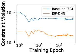
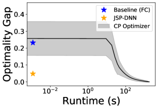
Figure 1: Constraint violations (left) and performance (right) of the baseline model (fully connected network trained with MSE loss) compared to the proposed JSP-DNN model. Benchmark: swv11. Constraint violation is the average magnitude of task overlap, measured with respect to the average processing time. The performance (right) reports the relative difference in makespan attained by the baseline and the JSP-DNN models, compared to an optimized version of IBM CP-optimizer over $30$ minutes.

This paper first presents the results of a baseline model whose approximation $\hat{\cal P}_{\bm{\theta}}$ is learned from a feed-forward ReLU network, named FC. The challenges of FC are illustrated in Figure 1, which reports the constraint violations (left) and the performance (right) of this baseline model compared to the proposed JSP-DNN model on the swv11 JSP benchmark instance of size $50\times 10$ (see Section 11 for details about the models and datasets). The left figure reports the non-overlap constraint violations measured as the relative task overlap with respect to the average processing time. While the baseline model often reports predictions whose corresponding makespans are close to the ground truth, the authors have observed that this model learns to “squeeze” schedules in order to reduce their makespans by allowing overlapping tasks. As a result this baseline model converges to solutions that violate the non-overlap constraint, often by very large amounts. The performance plot (right) shed additional light on the usability of this model in practice. It reports the time required by this baseline model to obtain a feasible solution (blue star) against the solution quality of a highly optimized solver (IBM CP-optimizer) over time. Obtaining feasible solutions efficiently is discussed in Section 10. The figures also report the constraint violations and solution quality found by the proposed JSS-DNN model (orange colors), which show dramatic improvements on both metrics. The next sections present the characteristics of JSS-DNN.

6 Capturing the JSS Constraints

To capture the JSS constraints within a deep learning model, a Lagrangian relaxation approach is used. Consider the optimization problem

$${\cal P}=\operatorname*{argmin}_{y}f(y)\;\;\mbox{subject to }\;\;g_{i}(y)\leq 0\;\;(\forall i\in[m]).$$ (2)

In Lagrangian relaxation, some or all the problem constraints are relaxed into the objective function using Lagrangian multipliers to capture the penalty induced by violating them. When all the constraints are relaxed, the Lagrangian function becomes

$$f_{\bm{\lambda}}(y)=f(y)+\sum_{i=1}^{m}\lambda_{i}g_{i}(y),$$ (3)

where the terms $\lambda_{i}\geq 0$ describe the Lagrangian multipliers, and $\bm{\lambda}=(\lambda_{1},\ldots,\lambda_{m})$ denotes the vector of all multipliers associated to the problem constraints. Note that, in this formulation, $g(y)$ can be positive or negative. An alternative formulation, used in augmented Lagrangian methods [13] and constraint programming [11], uses the following Lagrangian function

$$f_{\bm{\lambda}}(y)=f(y)+\sum_{i=1}^{m}\lambda_{i}\max(0,g_{i}(y)),$$ (4)

where the expressions $\max(0,g_{i}(y))$ capture a quantification of the constraint violations. When using a Lagrangian function, the optimization problem becomes

$$LR_{\bm{\lambda}}=\operatorname*{argmin}_{y}f_{\bm{\lambda}}(y),$$ (5)

and it satisfies $f(LR_{\bm{\lambda}})\leq f({\cal P})$. That is, the Lagrangian function is a lower bound for the original function. Finally, to obtain the strongest Lagrangian relaxation of ${\cal P}$, the Lagrangian dual can be used to find the best Lagrangian multipliers,

$$LD=\operatorname*{argmax}_{\bm{\lambda}\geq 0}f(LR_{\bm{\lambda}}).$$ (6)

For various classes of problems, the Lagrangian dual is a strong approximation of ${\cal P}$. Moreover, its optimal solutions can often be translated into high-quality feasible solutions by a post-processing step, which is the subject of Section 10.

This paper first presents the results of a baseline model whose approximation $\hat{\cal P}_{\bm{\theta}}$ is learned from a feed-forward ReLU network, named FC. The challenges of FC are illustrated in Figure 1, which reports the constraint violations (left) and the performance (right) of this baseline model compared to the proposed JSP-DNN model on the swv11 JSP benchmark instance of size $50\times 10$ (see Section 11 for details about the models and datasets). The left figure reports the non-overlap constraint violations measured as the relative task overlap with respect to the average processing time. While the baseline model often reports predictions whose corresponding makespans are close to the ground truth, the authors have observed that this model learns to “squeeze” schedules in order to reduce their makespans by allowing overlapping tasks. As a result this baseline model converges to solutions that violate the non-overlap constraint, often by very large amounts. The performance plot (right) shed additional light on the usability of this model in practice. It reports the time required by this baseline model to obtain a feasible solution (blue star) against the solution quality of a highly optimized solver (IBM CP-optimizer) over time. Obtaining feasible solutions efficiently is discussed in Section 10. The figures also report the constraint violations and solution quality found by the proposed JSS-DNN model (orange colors), which show dramatic improvements on both metrics. The next sections present the characteristics of JSS-DNN.

7 Capturing the JSP Constraints

To capture the JSP constraints within a deep learning model, a Lagrangian relaxation approach is used. Consider the optimization problem

$${\cal P}=\operatorname*{argmin}_{y}f(y)\;\;\mbox{subject to }\;\;g_{i}(y)\leq 0\;\;(\forall i\in[m]).$$ (7)

Its Lagrangian function is expressed as

$$f_{\bm{\lambda}}(y)=f(y)+\sum_{i=1}^{m}\lambda_{i}\max(0,g_{i}(y)),$$ (8)

where the terms $\lambda_{i}\geq 0$ describe the Lagrangian multipliers, and $\bm{\lambda}=(\lambda_{1},\ldots,\lambda_{m})$ denotes the vector of all multipliers associated with the problem constraints. In this formulation, the expressions $\max(0,g_{i}(y))$ capture a quantification of the constraint violations, which are often exploited in augmented Lagrangian methods [13] and constraint programming [11].

When using a Lagrangian function, the optimization problem becomes

$$LR_{\bm{\lambda}}=\operatorname*{argmin}_{y}f_{\bm{\lambda}}(y),$$ (9)

and it satisfies $f(LR_{\bm{\lambda}})\leq f({\cal P})$. That is, the Lagrangian function is a lower bound for the original function. Finally, to obtain the strongest Lagrangian relaxation of ${\cal P}$, the Lagrangian dual can be used to find the best Lagrangian multipliers,

$$\textstyle LD=\operatorname*{argmax}_{\bm{\lambda}\geq 0}f(LR_{\bm{\lambda}}).$$ (10)

For various classes of problems, the Lagrangian dual is a strong approximation of ${\cal P}$. Moreover, its optimal solutions can often be translated into high-quality feasible solutions by a post-processing step, which is the subject of Section 10.

7.1 Augmented Lagrangian of the JSP Constraints

Given an enumeration of the JSP constraints, the violation degree of constraint $i$ is represented by $\max(0,g_{i}(\bm{y}))$. Given the predicted values $\hat{\bm{s}}$, the violation degrees associated with the JSP constraints are expressed as follows:

$$\nu_{2b}\left(\hat{s}_{t}^{j}\right)=\max\left(0,\hat{s}_{t}^{j}+d_{t}^{j}-\hat{s}_{t+1}^{j}\right)$$ (11a)

$$\nu_{2c}\left(\hat{s}_{t}^{j},\hat{s}_{t^{\prime}}^{j^{\prime}}\right)=\min\left(\nu_{2c}^{L}\left(\hat{s}_{t}^{j},\hat{s}_{t^{\prime}}^{j^{\prime}}\right),\nu_{2c}^{R}\left(\hat{s}_{t}^{j},\hat{s}_{t^{\prime}}^{j^{\prime}}\right)\right),$$ (11b)

for the same indices as in Constraints (2b) and (2c) respectively, where

$$\nu_{2c}^{L}\left(\hat{s}_{t}^{j},\hat{s}_{t^{\prime}}^{j^{\prime}}\right) =\max\left(0,\hat{s}_{t}^{j}+d^{t}_{j}-\hat{s}_{t^{\prime}}^{j^{\prime}}\right)$$

$$\nu_{2c}^{R}\left(\hat{s}_{t}^{j},\hat{s}_{t^{\prime}}^{j^{\prime}}\right) =\max\left(0,\hat{s}_{t^{\prime}}^{j^{\prime}}+d^{t^{\prime}}_{j^{\prime}}-\hat{s}_{t}^{j}\right).$$

The term $\nu_{2b}$ refers to the task-precedence constraint (2b), and the violation degree $\nu_{2c}$ refers to the disjunctive non-overlap constraint (2c), with $\nu_{2c}^{L}$ and $\nu_{2c}^{R}$ referring to the two disjunctive components. When two tasks indexed $(j,t)$ and $(j^{\prime},t^{\prime})$ are scheduled on the same machine, if both disjunctions are violated, the overall violation degree $\nu_{2c}$ is considered to be the smaller of the two degrees, since this is the minimum distance that a task must be moved to restore feasibility.

7.2 The Learning Loss Function

The loss function of the learning model used to train the proposed JSP-DNN can now be augmented with the Lagrangian terms and expressed as follows:

$${\cal L}(\bm{s},\hat{\bm{s}},\bm{d})={\cal L}(\bm{s},\hat{\bm{s}})+\sum_{c\in{\cal C}}\lambda_{c}\nu_{c}(\hat{\bm{s}},\bm{d}).$$ (12)

It minimizes the prediction loss–defined as mean squared error between the optimal start times $\bm{s}$ and the predicted ones $\hat{\bm{s}}$–and it includes the Lagrangian relaxation based on the violation degrees $\nu$ of the JSP constraints $c\in{\cal C}$.

8 The Learning Model

Let $\hat{\cal P}_{\bm{\theta}}$ be the resulting JSS-DNN with parameters $\bm{\theta}$ and let ${\cal L}[\bm{\lambda}]$ be the loss function parametrized by the Lagrangian multipliers $\bm{\lambda}=\{\lambda_{c}\}_{c\in{\cal C}}$. The core training aims at finding the weights $\bm{\theta}$ that minimize the loss function for a given set of Lagrangian multipliers, i.e., it computes

$${\it LR}_{\bm{\lambda}}=\min_{\bm{\theta}}{\cal L}[\bm{\lambda}]\left(\bm{s},\hat{\cal P}_{{\bm{\theta}}}(\bm{d})\right).$$

In addition, JSS-DNN exploits Lagrangian duality to obtain the optimal Lagrangian multipliers, i.e., it solves

$${\it LD}=\max_{\bm{\lambda}}{\it LR}_{\bm{\lambda}}.$$

The Lagrangian dual is solved through a subgradient method that computes a sequence of multipliers $\bm{\lambda}^{1},\ldots,\bm{\lambda}^{k},\ldots$ by solving a sequence of trainings ${\it LR}_{\bm{\lambda}}^{0},\ldots,{\it LR}_{\bm{\lambda}}^{k-1},\ldots$ and adjusting the multipliers using the violations,

$$\bm{\theta}^{k+1} =\operatorname*{argmin}_{\bm{\theta}}{\cal L}[\bm{\lambda}^{k}]\left(\bm{s},\hat{\cal P}_{{\bm{\theta}}^{k}}(\bm{s})\right)$$ (L1)

$$\bm{\lambda}^{k+1} =\left(\lambda^{k}_{c}+\rho\,\nu_{c}\left(\hat{\cal P}_{{\bm{\theta}}^{k+1}}(\bm{s}),\bm{d}\right)\;|\;c\in{\cal C}\right),$$ (L2)

where $\rho>0$ is the Lagrangian step size. In the implementation, step (L1) is approximated using a Stochastic Gradient Descent (SGD) method. Importantly, this step does not recompute the training from scratch but uses a warm start for the model parameters $\bm{\theta}$.

input : ${\cal D},\alpha,\rho:$ Training data, Optimizer, and Lagrangian step sizes, reps.​​​​​​​​​​

$\bm{\lambda}^{0}\leftarrow 0\;\;\forall c\in{\cal C}$

for epoch $k=0,1,\ldots$ do

       foreach $(\bm{d},\bm{s})\!\leftarrow\!\mbox{minibatch}({\cal D})$ of size $b$ do

             $\hat{\bm{s}}\leftarrow\hat{\cal P}_{\bm{\theta}}(\bm{d})$

             ${\cal L}(\bm{s},\hat{\bm{s}})\leftarrow\frac{1}{b}\sum_{i\in[b]}{\cal L}\left(\bm{s}_{i},\hat{\bm{s}}_{i}\right)+\sum_{c\in{\cal C}}\lambda_{c}^{k}\nu_{c}\left(\bm{d}_{i},\hat{\bm{s}}_{i}\right)$​​​​​​​​​​

             $\theta\leftarrow\theta-\alpha\nabla_{\theta}\left({\cal L}(\bm{s},\hat{\bm{s}})\right)$

      foreach $c\in{\cal C}$ do

             $\lambda^{k+1}_{c}\leftarrow\lambda^{k}+\rho\nu_{c}\left(\bm{d},\hat{\bm{s}}\right)$

      

Algorithm 1 Learning Step

The overall training scheme is presented in Algorithm 1. It takes as input the training dataset ${\cal D}$, the optimizer step size $\alpha>0$ and the Lagrangian step size $\rho>0$. The Lagrangian multipliers are initialized in line 1. The training is performed for a fixed number of epochs, and each epoch optimizes the weights using a minibatch of size $b$. After predicting the task start times (line 1), it computes the objective and constraint losses (line 1). The latter uses the Lagrangian multipliers $\bm{\lambda}^{k}$ associated with current epoch $k$. The model weights $\theta$ are updated in line 1. Finally, after each epoch, the Lagrangian multipliers are updated following step (L2) described above (lines 1 and 1).

9 The JM-structured Network Architecture

This section describes the bespoke neural network architecture that exploits the JSP structure. Let $\mathcal{I}^{(m)}_{k}$ and $\mathcal{I}^{(j)}_{k}$ denote, respectively, the set of task indexes associated with the $k^{\text{th}}$ machine and the $k^{\text{th}}$ job. Further, denote with $\bm{d}[\mathcal{I}]$ the set of processing times associated with the tasks identified by index set $\mathcal{I}$. The JSP-structured architecture, called JM as for Jobs-Machines, is outlined in Figure 2. The network differentiates three types of layers: Job layers, that process processing times organized by jobs, Machine layers, that process processing times organized by machines, and Shared layers, that process the outputs of the job layers and the machine layers to return a prediction $\hat{\bm{s}}$.

The input layers are depicted with white rectangles. Each job layer $k$ takes as input the task processing times $\bm{d}[\mathcal{I}^{(j)}_{k}]$ associated with an index set $\mathcal{I}^{(j)}_{k}$ $(k\in[J])$, and each machine layer $k$ takes as input the task processing times $\bm{d}[\mathcal{I}^{(m)}_{k}]$ associated with an index set $\mathcal{I}^{(m)}_{k}$ $(k\in[J])$. The shared layers combine the latent outputs of the job and machine layers. A decoder-encoder pattern follows for each individual group of layers, which are fully connected and use ReLU activation functions (additional details are reported in Section 11).

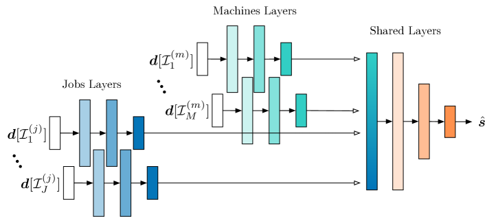
Figure 2: The JM Network Architecture of JSS-DNN.

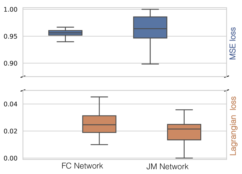
Figure 3: Distribution of No-Overlap Violation results corresponding to the hyperparameter search of Table 1.

The effect of the JM architecture is twofold. First, the patterns created by the job layers and the machine layers reflect the task-precedence and no-overlap structure of the JSP, respectively, encouraging the prediction to account for these constraints. Second, in comparison to an architecture that takes as input the full vector $\bm{d}$ and process it using fully connected ReLU layers, the proposed structure reduces the number of trainable parameters, as no connection is created within any two hidden layers processing tasks on different machines (machine layers) or jobs (job layers). This allows for faster convergence to high-quality predictions.

Figure 3 compares the no-overlap constraint violations resulting from each choice of loss function and network architecture over the whole range of hyperparameters searched. It uses benchmark ta30 and compares the Lagrangian dual results (orange/bottom) against a baseline using MSE loss (blue/top). It additionally compares the JM network architecture (right) against a baseline fully connected (FC) network (left). The results are scaled between $0$ (min) and $1$ (max). The figure clearly illustrates the benefits of using the Lagrangian dual method, and that the best results are obtained when the Lagrangian dual method is used in conjunction with the JM architecture. The results for task precedence constraints are analogous.

10 Constructing Feasible Solutions

It remains to show how to recover a feasible solution from the prediction. The recovery method exploits the fact that, given a task ordering on each machine, it is possible to construct a feasible schedule in low polynomial time. Moreover, a prediction $\hat{\bm{s}}$ defines implicitly a task ordering. Indeed, using $(j,t)$ to denote task $t$ of job $j$, a start time prediction vector $\hat{\bm{s}}$ can be used to define a task ordering $\preceq$ between tasks executing on the same machine, i.e.,

$$(j,t)\preceq_{\hat{\bm{s}}}(j^{\prime},t^{\prime})\;\;\text{iff}\;\;\hat{\mu}_{t}^{j}\leq\hat{\mu}_{t^{\prime}}^{j^{\prime}}\;\land\;\sigma_{t}^{j}=\sigma_{t^{\prime}}^{j^{\prime}},$$

where $\hat{\mu}_{t}^{j}=\frac{\hat{s}_{t}^{j}+d^{j}_{t}}{2}$ is the predicted midpoint of a task $t$ of job $j$.

Model 2 Recovering a Feasible Solution to the JSP.

$$\Pi(\bm{s}) ={\operatorname*{argmin}}_{\bm{s}}\;\;u$$

$$\mbox{subject to:}\;\;\eqref{con:2a},\eqref{con:2b}\;\;$$

$$s_{t}^{j}\geq s_{t^{\prime}}^{j^{\prime}}+{d}_{t^{\prime}}^{j^{\prime}}\;\;\forall j,j^{\prime}\!\in\![J],t,t^{\prime}\!\in\![T]\;\text{s.t.}\;(j,t)\preceq_{\hat{\bm{s}}}(j^{\prime},t^{\prime})$$ (13a)

$$s_{t}^{j}\geq 0\;\;\forall j\!\in\![J],t\!\in\![T]$$ (13b)

The Linear Program (LP) described in Model 2 computes the optimal schedule subject to the ordering $\preceq_{\hat{\bm{s}}}$ associated with prediction $\hat{\bm{s}}$. This LP has the same objective as the original scheduling problem, along with the upper bound on start times and task-precedence constraints. The disjunctive constraints of the JSP however are replaced by additional precedence constraints (13a) and (13b) for the ordering on each machine. The problem is totally unimodular when the durations are integral.

Input: $\{\hat{s}_{t}^{j}\}_{t\in[T],j\in[J]}$: predicted start times

$Q\leftarrow\text{enqueue}((j,1))$, $\;\;\forall j\in[J]$

while $Q$ is empty do

       $(j,t)\leftarrow\text{dequeue}(Q)$

       Schedule task $(j,t)$ with start time $\hat{s}^{j}_{t}$

       if $t<T$ then

             $\hat{s}_{t+1}^{j}\leftarrow\max(\hat{s}_{t+1}^{j},\hat{s}_{t}^{j}+d_{t}^{j})$

             $Q\leftarrow\text{enqueue}(j,t)$

       end if

      foreach  $(t^{\prime},j^{\prime})\text{ s.t. }t\neq t^{\prime}\;\land\;\sigma_{t^{\prime}}^{j^{\prime}}=\sigma_{t}^{j}\;\land\;\hat{s}_{t^{\prime}}^{j^{\prime}}\geq\hat{s}_{t}^{j}$ do

             $\hat{s}_{t^{\prime}}^{j^{\prime}}\leftarrow\max(\hat{s}_{t^{\prime}}^{j^{\prime}},\hat{s}_{t}^{j}+d_{t}^{j})$

       end foreach

      

end while

Algorithm 2 The JSP Greedy Recovery.

Note that the above LP may be infeasible: the machine precedence constraints may not be consistent with the job precedence constraints. If this happens, it is possible to use a greedy recovery algorithm that selects the next task to schedule based on its predicted starting time and updates predictions with precedence and machine constraints. The greedy procedure is illustrated in Algorithm 2 and is organized around a priority queue which is initialized with the first task in each job. Each iteration selects the task with the smallest starting time $\hat{s}_{t}^{j}$ and updates the starting of its job successor (line 6) and the starting times of the unscheduled task using the same machine (line 10). It is important to note that this greedy procedure was never needed: all test cases (e.g., all instances under all hyper-parameter combinations) induced machine orderings that were consistent with the job precedence constraints.

Remark on Learning Task Orderings

JSS-DNN learns to predict schedules as assignments of start times to each task. Another option would have been to learn machine orderings directly in the form of permutations since, once machine orderings are available, it is easy to recover start times. However, learning permutations was found to be much more challenging due to its less efficient representation of solutions. For example, for a $50\times 10$ JSP, predicting task ordering (or, equivalently, rankings) requires an output dimension of $50\times 50\times 10$ (a one-hot encoding to rank each of the $50$ tasks and $10$ machines). In contrast, the start time prediction requires only one value for each start-time, in this case, $50\times 10$. Enforcing feasibility also becomes more challenging in the case of rankings. It nontrivial to design successful violation penalties for task precedence constraints when using the one-hot encoding representation of the solutions.

Start times are easier to predict and indirectly produce good proxies for machine orderings.

11 Experimental Results

Parameter	Min Value	Max Value	Parameter	Min Value	Max Value
Learning Rate $\alpha$	0.000125	0.002	# Shared Layers	$2$	$2$
Dual Learning Rate $\rho$	0.001	0.05	Machine Layer Size	$2J$	$2J$
# Machine Layers	$2$	$2$	Job Layer Size	$2M$	$2M$
# Job Layers	$2$	$2$	Shared Layer Size	$2JM$	$2JM$

Table 1: Model Parameters and Hyper-Parameters.

Instance	Size	Prediction Err($\times 10$) $\downarrow$		Constraint Viol($\times 10^{2}$) $\downarrow$		Opt. Gap Heuristics (%) $\downarrow$					Opt. Gap DNNs (%) $\downarrow$		Time SoTA Eq. (s) $\uparrow$
	$J\times M$	FC	JSP-DNN	FC	JSP-DNN	SPT	LWR	MWR	LOR	MOR	FC	JSP-DNN	FC	JSP-DNN
yn02	$20\!\times\!20$	2.770	0.138	1.134	0.122	628	837	40	934	40	12.80 $\pm$ 5.4	-0.045 $\pm$ 0.9	10.20	1800+
ta25	$20\!\times\!20$	1.607	0.361	0.631	0.244	593	877	59	787	46	13.61 $\pm$ 3.13	-0.143 $\pm$ 0.8	11.02	1800+
ta30	$30\!\times\!15$	4.338	1.196	1.483	0.357	558	910	63	856	46	15.01 $\pm$ 2.63	-0.48 $\pm$ 5.18	9.06	1800+
ta40	$30\!\times\!20$	7.880	3.341	1.863	0.104	492	794	57	836	25	23.11 $\pm$ 7.33	3.19 $\pm$ 1.88	8.40	12.04
ta50	$50\!\times\!10$	4.580	1.322	1.223	0.225	789	789	53	1116	43	18.30 $\pm$ 5.22	5.85$\pm$ 2.72	8.02	90.30
swv03	$20\!\times\!15$	9.473	2.683	2.777	0.850	203	212	75	190	50	28.61 $\pm$ 14.27	7.62 $\pm$ 2.51	4.04	36.36
swv05	$20\!\times\!10$	6.586	2.950	2.325	0.626	183	192	80	177	66	20.78 $\pm$ 10.54	6.34 $\pm$ 1.82	7.24	18.18
swv07	$20\!\times\!10$	4.587	0.681	1.222	0.223	299	295	68	352	43	10.69 $\pm$ 6.83	0.01$\pm$ 4.75	26.0	254.5
swv09	$20\!\times\!15$	5.678	3.462	2.132	0.211	322	270	69	285	75	22.12 $\pm$ 8.52	5.42 $\pm$ 1.21	6.48	28.32
swv11	$50\!\times\!10$	7.958	3.244	2.711	0.282	237	231	94	263	73	23.18 $\pm$ 2.27	4.80 $\pm$ 4.47	7.02	92.00
swv13	$50\!\times\!10$	23.21	3.557	1.615	0.323	225	203	114	218	79	22.79 $\pm$ 16.21	8.11 $\pm$ 4.20	7.08	24.08

Table 2: Accuracy metrics compared between FC and JSP-DNN (left sub-table) and accuracy of simple heuristics vs CP-Optimizer at 1800s (right sub-table). Best results shown in bold.

The experiments evaluate JSS-DNN against the baseline FC network, the state-of-the-art CP commercial solver IBM CP-Optimizer, and several well-known scheduling heuristics.

Data Generation and Model Details

A single instance of the JSP with $J$ jobs and $M$ machines is defined by a set of assignments of tasks to machines, along with processing times required by each task. The generation of JSP instances simulates a situation in which a scheduling system experiences an unexpected “slowdown” on some arbitrary machine, inducing an increase in the processing times of each task assigned to the impaired machine. To create each experimental dataset, a root instance is chosen from the JSPLIB repository [29], and a set of $5000$ individual problem instances are generated accordingly, with all processing times on the slowdown machines extended from their original value to a maximum increase of $50$ percent. Each such instance is solved using the IBM CP-Optimizer constraint-programming software [22] with a time limit of 1800s. The instance and its solution are included in the training dataset.

Model Configuration

To ensure a fair analysis, the learning models have the same number of trainable parameters. The JM-structured neural networks are given two decoder layers per job and machine, whose sizes are twice as large as their corresponding numbers of tasks. These decoders are connected to a single Shared Layer (of size $2\times J\times M$). A final output layer, representing task start times, has size equal to the number of tasks in the JSP instance. The baseline fully connected networks are given $3$ hidden layers, whose sizes are chosen to match the the size of the corresponding JSS-DNN network in terms of the total number of parameters. The experiments apply the recovery operators discussed in the previous section to both the FC and JSS-DNN models to obtain feasible solutions from their predictions.

Time required for training and for running the models are reported in Appendix A.

The learning models are configured by a hyper-parameter search for the values summarized in Table 1. The search samples evenly spaced learning rates between their minimum and maximum values, along with similarly chosen dual learning rates $\rho$ when the Lagrangian loss function is used. Additionally, each configuration is evaluated with $5$ distinct random seeds, which primarily influences the neural network parameter initialization. The model with the best predicted schedules in average is selected for the experimental evaluation.

11.1 Model Accuracy and Constraint Violations

Table 2 represents the performance of the selected models. Each reported performance metric is averaged over the entire test set. For each prediction metric, symbols $\downarrow$ and $\uparrow$ indicates whether lower or higher values are better, respectively. The evaluation uses a $80$:$20$ split with the training data.

$\bullet$ Prediction Error $\downarrow$ The columns for prediction errors report the error between a predicted schedule and its target solution (before recovering a feasible solution). It is measured as the L1 distance between respective start times. The predictions by JSS-DNN are much closer to the targets than those of the FC model. JSS-DNN reduces the errors by up to an order of magnitude compared to FC, demonstrating the ability of the JM architecture and the Lagrangian dual method to exploit the problem structure to derive good predictions.

$\bullet$ Constraint Violation $\downarrow$ The constraint violations are collected before recovering a feasible solution and the columns report the average magnitude of overlap between two tasks as a fraction of the average processing time. The results show again that the violation magnitudes reported by JSS-DNN are typically one order of magnitude lower than those reported by FC. They highlight the effectiveness of the Lagrangian dual approach to take into account the problem constraints.

$\bullet$ Optimality Gap $\downarrow$ The quality of the predictions is measured as the average relative difference between the makespan of the feasible solutions recovered from the predictions of the deep-learning models, and the makespan obtained by the IBM CP-Optimizer with a timeout limit of $1800$ seconds. The optimality gap is the primary measure of solution quality, as the goal is to predict solutions to JSP instances that are as close to optimal as possible. The table also reports the optimality gaps achieved by several (fast) heuristics, relative to the same CP-Optimizer baseline. They are Shortest Processing Time (SPT), Least Work Remaining (LWR), Most Work Remaining (MWR), Least Operations Remaining (LOR), and Most Operations Remaining (MOR). Since the CP solver cannot typically find optimal solutions within the given timeout, the results under-approximate the true optimality gaps.

The results show that the proposed JSS-DNN substantially outperforms all other heuristic baselines and the best FC network of equal capacity. On these difficult instances, the most accurate heuristics exhibit results whose relative errors are at least an order of magnitude larger than those of JSS-DNN. Similarly, JSS-DNN significantly outperforms FC.

It is interesting to observe that, for instances yn02, ta25, and ta30, the makespan of the recovered JSS-DNN solutions outperform, on average, those reported by the CP solver before it reaches its time limit, which is quite remarkable. The CP solver can actually produce these solutions as well if it is allowed to run for several hours. This opens an interesting avenue beyond for further research: the use of JSS-DNN to hot-start a CP solver.

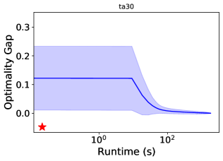
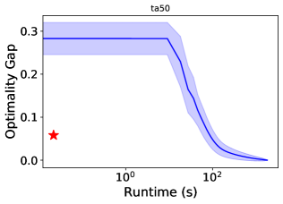
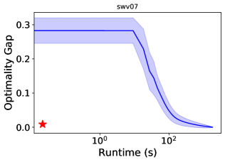
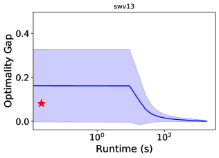
Figure 4: Comparison of mean timing and accuracy of four JSS-DNN models (red) against CP-optimizer mean optima and standard deviation (blue).

11.2 Comparison with SoTA Solver $\uparrow$

The last results compare JSS-DNN and the state-of-the art CP solver in terms of their ability to find high-quality solutions quickly. The runtime of JSS-DNN is dominated by the solution recovery process (Model 2 and Algorithm 2): their runtimes depend on the instance size but never exceed $30$ms for the test cases.

The results are depicted in the last two columns of Table 2. They report the average runtimes required by the CP solver to produce solutions that match or outperform the feasible (recovered) solutions produced by JSS-DNN and FC. The results show that it takes the CP solver less than 12 seconds to outperform FC. In contrast, the CP solver takes at least an order of magnitude longer to outperform JSS-DNN and is not able to do so within 30 minutes on the first 3 test cases.

Figure 4 complements these results on three test cases: they depict the evolution of the makespan produced by the CP solver over time and contrast these with the solution recovered by JSS-DNN. The thick line depicts the mean makespan, the shaded region captures its standard deviation, and the red star reports the quality of the JSS-DNN solution. These results highlight the ability of JSS-DNN to generate a high-quality solution quickly.

Overall, these results show that JSS-DNN may be a useful addition to the set of optimization tools for scheduling applications that require high-quality solutions in real time. It may also provide an interesting avenue to seed optimization solvers, as mentioned earlier.

12 Conclusions

This paper proposed JSS-DNN, a deep-learning approach to produce high-quality approximations of Job shop Scheduling Problems (JSPs) in milliseconds. The proposed approach combines deep learning and Lagrangian duality to model the combinatorial constraints of the JSP. It further exploits the JSP structure through the design of dedicated neural network architectures to reflect the nature of the task-precedence and no-overlap structure of the JSP, encouraging the predictions to take account of these constraints. The paper also presented efficient recovery techniques to post-process JSS-DNN predictions and produce feasible solutions. The experimental analysis showed that JSS-DNN produces feasible solutions whose quality is at least an order of magnitude better than commonly used heuristics. Moreover, a state-of-the-art commercial CP solver was shown to take a significant amount of time to obtain solutions of the same quality and may not be able to do so within 30 minutes on some test cases.

Appendix A Timing Results

In the models described in this paper, the size of each DNN layer depends on the size of the corresponding benchmark JSP instance, as do the number of constraints to be enforced. These factors influence the computational runtime of each component model and the associated training. Table 3 presents the time required to train for $1$ epoch, the total training time taken to train each model, the time required to run inference on $1$ sample, and the time required to construct feasible solutions using Model 2. All results are reported on average.

Benchmark	Training ($1$ Epoch) (s)	Training (Total) (s)	Inference (s) ($\times 10^{3}$)	Model 2 (s)
yn02	2.306	1153	3.7	0.0152
ta25	2.102	1051	3.7	0.0155
ta30	2.232	1116	5.0	0.0160
ta40	2.914	1457	4.2	0.0171
ta50	4.452	2226	7.5	0.0301
swv03	1.377	688	2.9	0.0095
swv05	1.335	668	3.5	0.0086
swv07	2.135	1067	3.1	0.0122
swv09	2.014	1007	3.1	0.0121
swv11	5.018	2509	5.3	0.0213
swv13	5.233	2617	5.4	0.0215

Table 3: Runtime for Model Training and Execution.

Appendix B Technical Specifications

All computations involved in this work were performed on the following platform: Intel(R) Xeon(R) Platinum 8260 CPU @ 2.40GHz. The operating system used throughout was Ubuntu 20.04.2 LTS, along with Python $3.7.6$, Pytorch $1.4.0$, Numpy $1.20.3$, Google OR-Tools $8.0.8283$, and IBM ILOG CP Optimizer Developer Edition $12.10$.

Appendix C Code and Data

All training datasets consist of $5000$ individual JSP instances, beginning with a root benchmark instance and with uniformly increased processing times on one machine, from $1$ to $1.5$ times the original duration. Each instance is solved using the CP Optimizer software with a time limit of $30$ minutes. To control for the existence of symmetries, i.e. co-optimal solutions, each solved instance is post-processed to minimize the $L^{1}$ distance from its schedule to that of the next instance, with respect to increasing processing times. All code used to produce this project will be released upon publication.

Appendix D Final Hyperparameters

Table 4 presents the final hyperparameters used for each benchmark instance and model to produce the results of Table 2.

Benchmark	Learning Rate (Baseline/FC)	Learning Rate (JSP-DNN)	Dual Learning Rate (JSP-DNN)
yn02	0.002667	0.009432	0.001
ta25	0.01	0.004141	0.001
ta30	0.01	0.004141	0.001
ta40	0.01	0.01	0.01
ta50	0.000833	0.001797	0.001
swv03	0.0045	0.001797	0.001
swv05	0.0045	0.007515	0.001
swv07	0.000833	0.004141	0.05
swv09	0.01	0.001797	0.001
swv11	0.008167	0.002386	0.001
swv13	0.001	0.001797	0.001

Table 4: Final Hyperprarmeters used.

References

- Agarwal et al. [2018] A. Agarwal, A. Beygelzimer, M. Dudík, J. Langford, and H. Wallach. A reductions approach to fair classification. arXiv preprint arXiv:1803.02453, 2018.
- Amos and Kolter [2017a] B. Amos and J. Z. Kolter. Optnet: Differentiable optimization as a layer in neural networks. In ICML, pages 136–145. JMLR. org, 2017a.
- Amos and Kolter [2017b] B. Amos and J. Z. Kolter. Optnet: Differentiable optimization as a layer in neural networks. In International Conference on Machine Learning, pages 136–145. PMLR, 2017b.
- Arora et al. [2012] S. Arora, E. Hazan, and S. Kale. The multiplicative weights update method: a meta-algorithm and applications. Theory of Computing, 8(1):121–164, 2012.
- Balcan et al. [2018] M.-F. Balcan, T. Dick, T. Sandholm, and E. Vitercik. Learning to branch. In International conference on machine learning, pages 344–353. PMLR, 2018.
- Bengio et al. [2020] Y. Bengio, A. Lodi, and A. Prouvost. Machine learning for combinatorial optimization: a methodological tour d’horizon. European Journal of Operational Research, 2020.
- Cotter et al. [2018] A. Cotter, M. Gupta, H. Jiang, N. Srebro, K. Sridharan, S. Wang, B. Woodworth, and S. You. Training well-generalizing classifiers for fairness metrics and other data-dependent constraints. arXiv preprint arXiv:1807.00028, 2018.
- Donti et al. [2017] P. Donti, B. Amos, and J. Z. Kolter. Task-based end-to-end model learning in stochastic optimization. In NIPS, pages 5484–5494, 2017.
- Fioretto et al. [2020a] F. Fioretto, P. V. Hentenryck, T. W. K. Mak, C. Tran, F. Baldo, and M. Lombardi. Lagrangian duality for constrained deep learning. In Machine Learning and Knowledge Discovery in Databases. Applied Data Science and Demo Track - European Conference, ECML PKDD, volume 12461 of Lecture Notes in Computer Science, pages 118–135. Springer, 2020a.
- Fioretto et al. [2020b] F. Fioretto, T. W. K. Mak, and P. V. Hentenryck. Predicting AC optimal power flows: Combining deep learning and lagrangian dual methods. In Proceedings of the AAAI Conference on Artificial Intelligence, pages 630–637, 2020b.
- Fontaine et al. [2014] D. Fontaine, M. Laurent, and P. Van Hentenryck. Constraint-based lagrangian relaxation. In Principles and Practice of Constraint Programming, pages 324–339, 2014.
- Gombolay et al. [2018] M. Gombolay, R. Jensen, J. Stigile, T. Golen, N. Shah, S.-H. Son, and J. Shah. Human-machine collaborative optimization via apprenticeship scheduling. Journal of Artificial Intelligence Research, 63:1–49, 2018.
- Hestenes [1969] M. R. Hestenes. Multiplier and gradient methods. Journal of optimization theory and applications, 4(5):303–320, 1969.
- Kan [2012] A. R. Kan. Machine scheduling problems: classification, complexity and computations. Springer Science & Business Media, 2012.
- Kearns et al. [2017] M. Kearns, S. Neel, A. Roth, and Z. S. Wu. Preventing fairness gerrymandering: Auditing and learning for subgroup fairness. arXiv:1711.05144, 2017.
- Khalil et al. [2016] E. Khalil, P. Le Bodic, L. Song, G. Nemhauser, and B. Dilkina. Learning to branch in mixed integer programming. In Proceedings of the AAAI Conference on Artificial Intelligence, volume 30, 2016.
- Khalil et al. [2017] E. Khalil, H. Dai, Y. Zhang, B. Dilkina, and L. Song. Learning combinatorial optimization algorithms over graphs. In NIPS, pages 6348–6358, 2017.
- Kool et al. [2018] W. Kool, H. Van Hoof, and M. Welling. Attention, learn to solve routing problems! arXiv preprint arXiv:1803.08475, 2018.
- Kotary et al. [2021a] J. Kotary, F. Fioretto, P. V. Hentenryck, and B. Wilder. End-to-end constrained optimization learning: A survey. In Z. Zhou, editor, Proceedings of the Thirtieth International Joint Conference on Artificial Intelligence, IJCAI, pages 4475–4482. ijcai.org, 2021a.
- Kotary et al. [2021b] J. Kotary, F. Fioretto, P. Van Hentenryck, and B. Wilder. End-to-end constrained optimization learning: A survey. arXiv preprint arXiv:2103.16378, 2021b.
- Ku and Beck [2016] W.-Y. Ku and J. C. Beck. Mixed integer programming models for job shop scheduling: A computational analysis. Computers & Operations Research, 73:165–173, 2016.
- Laborie [2009] P. Laborie. Ibm ilog cp optimizer for detailed scheduling illustrated on three problems. In International Conference on AI and OR Techniques in Constriant Programming for Combinatorial Optimization Problems, pages 148–162. Springer, 2009.
- LeCun et al. [2015] Y. LeCun, Y. Bengio, and G. Hinton. Deep learning. Nature, 521:436–444, 2015.
- Mandi et al. [2020] J. Mandi, P. J. Stuckey, T. Guns, et al. Smart predict-and-optimize for hard combinatorial optimization problems. In Proceedings of the AAAI Conference on Artificial Intelligence (AAAI), volume 34, pages 1603–1610, 2020.
- Nair et al. [2020] V. Nair, S. Bartunov, F. Gimeno, I. von Glehn, P. Lichocki, I. Lobov, B. O’Donoghue, N. Sonnerat, C. Tjandraatmadja, P. Wang, et al. Solving mixed integer programs using neural networks. arXiv preprint arXiv:2012.13349, 2020.
- Narasimhan [2018] H. Narasimhan. Learning with complex loss functions and constraints. In International Conference on Artificial Intelligence and Statistics, pages 1646–1654, 2018.
- Nowak et al. [2018] A. Nowak, S. Villar, A. S. Bandeira, and J. Bruna. Revised note on learning algorithms for quadratic assignment with graph neural networks, 2018.
- Pogančić et al. [2020] M. V. Pogančić, A. Paulus, V. Musil, G. Martius, and M. Rolinek. Differentiation of blackbox combinatorial solvers. In International Conference on Learning Representations (ICLR), 2020.
- tamy0612 [2014] tamy0612. Jsplib: Benchmark instances for job-shop scheduling problem, Nov 2014. URL https://github.com/tamy0612/JSPLIB.
- Tran et al. [2021] C. Tran, F. Fioretto, and P. V. Hentenryck. Differentially private and fair deep learning: A lagrangian dual approach. In AAAI Conference on Artificial Intelligence, AAAI, pages 9932–9939. AAAI Press, 2021.
- Vesselinova et al. [2020] N. Vesselinova, R. Steinert, D. F. Perez-Ramirez, and M. Boman. Learning combinatorial optimization on graphs: A survey with applications to networking. IEEE Access, 8:120388–120416, 2020.
- Vinyals et al. [2015a] O. Vinyals, M. Fortunato, and N. Jaitly. Pointer networks. In NIPS, pages 2692–2700, 2015a.
- Vinyals et al. [2015b] O. Vinyals, M. Fortunato, and N. Jaitly. Pointer networks. In Advances in Neural Information Processing Systems (NeurIPS, pages 2692–2700, 2015b.
- Wilder et al. [2019a] B. Wilder, B. Dilkina, and M. Tambe. Melding the data-decisions pipeline: Decision-focused learning for combinatorial optimization. In Proceedings of the AAAI Conference on Artificial Intelligence (AAAI), volume 33, pages 1658–1665, 2019a.
- Wilder et al. [2019b] B. Wilder, B. Dilkina, and M. Tambe. Melding the data-decisions pipeline: Decision-focused learning for combinatorial optimization. In AAAI, volume 33, pages 1658–1665, 2019b.