Dislocation-based strength model for high energy density conditions

Abstract

We derive a continuum-level plasticity model for polycrystalline materials in the high energy density regime, based on a single dislocation density and single mobility mechanism, with an evolution model for the dislocation density. The model is formulated explicitly in terms of quantities connected closely with equation of state (EOS) theory, in particular the shear modulus and Einstein temperature, which reduces the number of unconstrained parameters while increasing the range of applicability. The least constrained component is the Peierls barrier $E_{P}$, which is however accessible by atomistic simulations. We demonstrate an efficient method to estimate the variation of $E_{P}$ with compression, constrained to fit a single flow stress datum. The formulation for dislocation mobility accounts for some or possibly all of the stiffening at high strain rates usually attributed to phonon drag. The configurational energy of the dislocations is accounted for explicitly, giving a self-consistent calculation of the conversion of plastic work to heat. The configurational energy is predicted to contribute to the mean pressure, and may reach several percent in the terapascal range, which may be significant when inferring scalar EOS data from dynamic loading experiments. The bulk elastic shear energy also contributes to the pressure, but appears to be much smaller. Although inherently describing the plastic relaxation of elastic strain, the model can be manipulated to estimate the flow stress as a function of mass density, temperature, and strain rate, which is convenient to compare with other models and inferences from experiment. The deduced flow stress reproduces systematic trends observed in elastic waves and instability growth experiments, and makes testable predictions of trends versus material and crystal type over a wide range of pressure and strain rate.

I Introduction

Overwhelmingly most research on plastic flow has been devoted to engineering materials and simpler variants such as elemental Fe and Al, for deformation rates and temperatures occurring in typical applications, and at pressures around ambient, or between zero and those occurring in high-pressure static reservoirs, which is essentially the same. However, strength is important in a much wider range of materials and conditions. An extreme example is the crust of neutron stars Horowitz2009 , where fracture causing a break in the crust, leading to magnetic reconnection, has been proposed as a mechanism for giant gamma ray bursts in magnetars, which are powerful enough to disturb the Earth’s ionosphere from tens of thousands of light years Campbell2005 . At the intersection of science and engineering are the impact of micrometeoroids on spacecraft, and experiments performed to investigate material properties at pressures into the terapascal scale during dynamic loading on nanosecond time scales hedexpts , which are directly relevant to the development of techniques for inertially-confined thermonuclear fusion icf . As well as the sample materials studied, these experiments usually involve other components whose strength often affects the conditions imparted to or inferred in the sample. Simulations and interpretation of these experiments then must rely on models of strength that have not been calibrated or validated in relevant conditions. Strength models can be deduced theoretically, but the detailed mechanisms of plastic flow are complicated, and have previously involved extensive multi-scale computational studies using electronic structure, molecular dynamics, and dislocation dynamics to calibrate a continuum-level model suitable for simulations of dynamic loading experiments Barton2011 ; Barton2013 . Successful plasticity models have also been developed by considering physically-plausible contributions for the motion and evolution of dislocations, and calibrating them primarily to experimental measurements probing the sensitivity to temperature, pressure, strain rate etc Preston2003 ; Rodriguez2011 ; Gao2012 ; Lim2015 ; Austin2018 . Dynamic loading experiments are difficult and expensive, and such models are usually calibrated over a narrow range of relatively low pressures. Otherwise, strength models used for such simulations are essentially empirical descriptions of the flow stress as a function of state, calibrated to much lower pressures, temperatures, and strain rates, with minor empirical or guessed modifications. One notable ad hoc simplification is that, in all widely-used continuum models, the heat imparted by flow against strength is assumed to be a constant fraction of the plastic work, often simply unity. In contrast, experimental measurements Mason1994 ; Kapoor1998 ; Soares2021 and theoretical studies Rosakis2000 ; Hodowany2000 ; Zubelewicz2008 ; Zubelewicz2019 have found that the fraction may vary between 0.1 or less to $\sim$1 over the course of a single loading event.

We have recently developed methods to predict several properties of matter efficiently over a wide range of states, including the equation of state (EOS) Swift_ajeos_2019 ; Swift_wdeos_2020 , the asymptotic freedom of ions leading to the drop in their heat capacity from 3 to $3/2\,k_{\text{B}}$ at high temperature Swift_iontherm_2020 , and also the shear modulus Swift_ajshear_2021 , which is the driving force behind plastic flow. We previously developed a dislocation-based crystal plasticity model for deformation at high pressures and strain rates, formulated with the intention of requiring less computational effort to calibrate Swift_xtplast_2008 . In the work reported here, we extend the concepts behind this model, informed by recent developments and experience, and combine it with our new predictions of shear modulus to produce a strength model valid potentially over the full range of normal matter, with particular interest in conditions occurring in high energy density (HED) applications such as loading induced by laser ablation.

We do not expect the model described here to be as accurate as models constructed from more detailed multi-scale studies over a more restricted range of states Barton2011 ; Barton2013 , or by considerating detailed energetics and kinematics of a dislocation, such as the bowing geometry, pinning, and cross-slip Lim2015 ; Hunter2015 ; Blaschke2020 ; Hunter2022 . However, the present model is significantly simpler to implement and calibrate, includes other effects neglected in previous strength models, and can be applied in arbitrarily extreme conditions without further extension or calibration. Although we use a particular electronic structure method to supply properties needed to infer the strength over a wide range of states, the plasticity model is constructed to make it straightforward to substitute properties calculated using more detailed or accurate methods where available. It is preferable to use a strength model constructed using potentially inaccurate components than one constructed to be accurate under irrelevant conditions that would definitely be inaccurate outwith its range of calibration, or no model at all. This approach may also be suitable to estimate the plastic flow rate associated with twinning, as this process also fundamentally involves atoms hopping past a Peierls barrier.

II Dislocation dynamics

In contrast to our previous study Swift_xtplast_2008 , we focus here on plastic flow in polycrystalline aggregates, omitting some effects such as the change in resolved shear stress from finite elastic strains, and employing implicit averages over crystal orientations and slip systems. The constitutive equations can be solved in different ways, influenced by the internal structure of simulation programs in which they are implemented. As before Swift_xtplast_2008 , the intended method of solution is in continuum dynamics simulations in which the local material state includes the elastic strain tensor, from which the stress tensor $\tau$ is calculated using the bulk and shear moduli $B$ and $G$, properties of the material state and in particular of the mass density $\rho$. $G$ can be predicted from electronic structure theory, as in our recent wide-range study Swift_ajshear_2021 . The driving force for plastic deformation is the deviatoric stress

$$\sigma\equiv\tau+Ip,$$ (1)

where the mean pressure $p=-\mbox{Tr}\,\tau/3$. The deviatoric stress $\sigma=G\epsilon_{e}$ where $\epsilon_{e}$ is the elastic strain deviator and $G$ the shear modulus. In finite-strain continuum mechanics, the isotropic and shear strain rates are the isotropic and deviatoric decomposition of the symmetric part of the gradient tensor of the material velocity field $\vec{u}(\vec{r})$:

$$\dot{\epsilon}\equiv\mbox{Symm}(\mbox{grad}\,\vec{u})+\dot{\mu}I,$$ (2)

the antisymmetric part describing rotation. The isotropic strain rate gives the rate of compression, $\dot{\mu}\equiv-\mbox{div}\,\vec{u}=\dot{\rho}/\rho$. The deviatoric strain rate $\dot{\epsilon}$ is the sum of elastic and plastic components. Here we use dislocation dynamics to determine the plastic strain rate. For polycrystal-averaged materials with shear stress calculated using a single, isotropic shear modulus, the scalar plastic strain rate $\dot{\epsilon}_{p}$ acts to reduce the elastic strain by radial relaxation toward the state of isotropic pressure. This approach is standard for continuum simulations of the response of matter to dynamic loading Benson1992 .

The plastic strain rate $\dot{\epsilon}_{p}$ is related to the dislocation density $\rho_{d}$ and the mean speed of dislocation motion $\bar{v}_{d}$ by a modified Orowan equation Barton2013

$$\dot{\epsilon}_{p}=\frac{\eta}{M}\rho_{d}b\bar{v}_{d}$$ (3)

where $b$ is the magnitude of the Burgers vector, $M$ the Taylor factor representing an effective number of active slip systems, and $\eta$ a microstructure factor representing the number of dislocation types (1 for screw only, 2 for screw and edge). $\bar{v}_{d}$ can be obtained from a kinetics model, giving a hopping rate $Z$, so $\bar{v}_{d}=bZ$. $\rho_{d}$ is usually defined in conventional metallurgical terms as the dislocation line length per volume of material. At finite compressions, $\rho_{d}$ and $b$ scale with the mass density $\rho$ as $\rho^{2/3}$ and $\rho^{-1/3}$ respectively. The constitutive equations become simpler, and more straightforward to generalize to large changes in compression, if expressed instead using the fraction of atoms on a dislocation,

$$\phi_{d}=\rho_{d}\frac{m_{a}}{b\rho}$$ (4)

where $m_{a}$ is the mass of an atom. Then

$$\dot{\epsilon}_{p}=\frac{\eta}{M}\phi_{d}Z\gamma\quad:\quad\gamma\equiv\frac{6f_{v}^{3}}{\pi}$$ (5)

The ratio of Burgers vector to Wigner-Seitz radius, $b/r_{\text{WS}}$, is constant for a given crystal structure (Table 1); for convenience we consider the distance from the equilibrium position to the peak of the Peierls barrier, $b/2$, as $f_{v}\equiv b/2r_{\text{WS}}$.

Table 1: Scaling between Burgers vector and Wigner-Seitz radius, for simple crystal structures.

structure	$f_{v}$
body-centered cubic (bcc)	$\frac{1}{2}\left(9\pi\right)^{1/3}$
face-centered cubic (fcc)	$\frac{1}{\sqrt{2}}\left(2\pi/3\right)^{1/3}$
hexagonal close-backed (hcp), basal	$\left(2\pi/3\right)^{1/3}$
diamond	$\frac{1}{\sqrt{2}}\left(4\pi/3\right)^{1/3}$

Previous dislocation-based strength models were constructed, and $\bar{v}_{d}$ calculated, assuming dislocation motion was impeded by barriers to ‘forward’ motion Preston2003 ; Barton2011 ; Barton2013 ; Austin2018 . The resulting Arrhenius hopping probability gives a non-zero $\bar{v}_{d}$ at zero applied stress, and various modifications have been employed to ensure that $\bar{v}\rightarrow 0$ as $\|\sigma\|\rightarrow 0$, including the use of an error function instead of an Arrhenius rate Preston2003 , and a minimum stress below which $\bar{v}_{d}$ was set to zero Barton2011 ; Barton2013 ; Austin2018 . As we pointed out previously Swift_xtplast_2008 , this problem is avoided by recognizing that atoms have no inherently preferred hopping direction, but the local stress field biases hops in the direction that reduces shear stress, because the stress reduces the Peierls barrier in that direction and increases it in the opposite direction. The resulting hopping rate is

$$Z=Z_{0}\left[\exp\left(-N\frac{E_{P}-E_{\tau}}{k_{\text{B}}T}\right)-\exp\left(-N\frac{E_{P}+E_{\tau}}{k_{\text{B}}T}\right)\right]$$ (6)

where $Z_{0}$ is the attempt rate, $E_{P}$ the Peierls barrier, $N$ the number of coordinated atom jumps required for the dislocation to move, $T$ the temperature, and $k_{\text{B}}$ Boltzmann’s constant. $E_{\tau}$ is the effect of the local stress on the forward and reverse Peierls barriers, $\|\sigma\|v_{\text{WS}}f_{v}$ where $v_{\text{WS}}$ is the Wigner-Seitz volume. As well as being numerically-better conditioned as $\sigma\rightarrow 0$, the inclusion of reverse hopping reduces the net rate at elevated temperatures, giving similar phenomenological behavior as has been attributed to phonon damping, but without an additional explicit contribution or parameters. The barrier-lowering effect of the applied stress for forward hopping has also been considered by other researchers Deo2005 , and the effect of reverse hopping has been included in dislocation based studies of creep Nichols1971 .

The Arrhenius rate itself represents the probability of an atom following a Maxwell-Boltzmann velocity distribution crossing a positive energy barrier greater than $k_{\text{B}}T$. If the stress is high enough for the barrier to become substantially smaller, the Arrhenius rate is incorrect; it should certainly not exceed unity. The mean dislocation speed is thus limited to $Z_{0}b$ at high stresses, just as the ‘relativistic’ effect attributed to phonon drag.

At the microstructural level, stress is resolved on the specific slip systems and stress relaxation occurs by the motion of dislocations of each Burgers vector, with separate kinetics for each. The resolved shear stress and Burgers vector occur in the exponent of the rate equation Eq. 6, so in principle the response of polycrystalline material may be non-linear with respect to averaging of the resolved stress in the exponent and averaging of the plastic strain rate: a potential source of inaccuracy in predicting the flow stress. This averaging could be performed explicitly for a given crystal structure to go beyond the use of an assumed Taylor factor, and multiple contributions to the rate could be included with different Peierls barriers and effective attempt rates, to account for non-Schmid effects even in an average polycrystalline model. For now, we simply take a constant value $M$ appropriate for the crystal structure and material.

Similarly, there are in general several barriers that affect the dislocation mobility, including the Peierls barrier for the ideal lattice, impurities such as interstitials, and intersections with dislocations of different Burgers vector. Usually one or other barrier dominates and controls the plastic strain rate, depending on the material, compression, temperature, applied stress, and microstructural state including the instantaneous dislocation density. In principle, several types of barrier could be incorporated even in a polycrystal-averaged model, potentially including competition between multiple slip systems leading to non-Schmid effects and a varying effective Taylor factor. In the present work, we consider a single barrier and investigate its applicability over a wide range of conditions in the HED regime.

III Evolution of dislocation density

The model so far gives the plastic strain rate for a given dislocation density. Predictions of the rate of change of shear stress can be made given a measurement of the initial dislocation density in a material, but the dislocation density evolves as plastic flow occurs. A key theoretical insight leading to dislocation-based plasticity models has been the prediction that, at a given strain rate, the dislocation density evolves rapidly toward an equilibrium value Barton2011 , which can be estimated from large-scale dislocation dynamics simulations and parameterized as part of the strength model. Here we investigate an approach in which the equilibrium density $\hat{\phi}_{d}$ is an emergent property rather than a separately-calibrated definition. Ignoring the spontaneous generation of dislocations, if dislocations are sufficiently far apart and thus unable to annihilate each other, and considering dislocation loops from Frank-Read type sources, the rate of dislocation generation is proportional to the rate of dislocation motion:

$$\dot{\phi}_{d}=\frac{\pi}{2}\frac{\phi_{d}}{M}Z=\frac{\pi}{2}\frac{\dot{\epsilon}_{p}}{\gamma}.$$ (7)

For a given slip system, if dislocations of opposite Burgers vector occur in equal numbers, one contribution to their annihilation is collision as they move in opposite directions under the applied stress. In addition, dislocations of opposite sign attract each other through their mutual elastic strain fields, which decay with distance from each dislocation as $Gb/r$. Using the same method for predicting the hopping rate as for the applied stress,

$$Z_{a}=Z_{0}\left[\exp\left(-N\frac{E_{P}-E_{m}}{k_{\text{B}}T}\right)-\exp\left(-N\frac{E_{P}+E_{m}}{k_{\text{B}}T}\right)\right]$$ (8)

where $E_{m}$ is the adjustment to the Peierls barrier from the mutual interaction field of the dislocations,

$$E_{m}=\frac{Gv_{\text{WS}}f_{v}}{\bar{L}}$$ (9)

where $\bar{L}$ is the mean separation between dislocations of opposite sign, in units of the Burgers vector,

$$\bar{L}=\sqrt{\frac{2M}{\phi_{d}}}.$$ (10)

The net rate of change in dislocation density is then

$$\dot{\phi}_{d}=\frac{\pi}{2}\frac{\phi_{d}}{M}Z\left(1-\frac{2}{\bar{L}}\right)-\frac{2\phi_{d}Z_{a}}{\bar{L}}=\frac{\dot{\epsilon}_{p}}{\gamma}\frac{\pi}{2}\left(1-\frac{2}{\bar{L}}\right)-\frac{2\phi_{d}Z_{a}}{\bar{L}}.$$ (11)

Adjustment factors may be included for each term to match more detailed modeling where available.

If the dislocation population is in equilibrium, $\dot{\phi}_{d}=0$, and $\hat{\phi}_{d}$ can be deduced from Eq. 11, which can be solved numerically by bisection since $0\leq\phi_{d}\leq 1$. Dependence on state and strain rate enters through the attraction term only. Neglecting this term,

$$\hat{\phi}_{d}=M/2>1.$$ (12)

This limiting case could be the result of over-simplification in the generation and collision terms, such as the use of the mean separation $\bar{L}$. There presumably is a limiting value of $\phi_{d}$, $\phi_{\text{max}}$ say, above which the concept of dislocations is meaningless. In practice, $\phi_{d}$ must remain well below 1 for the crystal lattice to be stable Cotterill1977 . To correct for too large a $\phi_{\text{max}}$ from the asymptotic limit of the generation and collision terms, we include an additional saturation term to limit $\phi_{d}$ to some chosen $\phi_{\text{max}}$:

$$\dot{\phi}_{d}=R_{m}(\phi_{\text{max}}-\phi_{d})-R_{c}-R_{a}$$ (13)

where $R_{m}$, $R_{c}$, and $R_{a}$ are the rates from multiplication, collision, and attraction respectively, from Eq. 11.

As we are neglecting homogeneous thermal nucleation of dislocations, the equilibrium dislocation density at static conditions $\hat{\phi}_{d}(\dot{\epsilon}_{p}=0)$ is zero. This is physically reasonable as the dislocation population in virtually all metals as prepared is metastable under ambient conditions. In practice, we can specify a reasonable value for the initial dislocation density, and find that evolution toward zero is negligible under ambient conditions on the time scales of HED experiments. The estimates of $\phi_{d}$ in-situ during dynamic deformation could be tested by experiments e.g. using synchrotron x-ray measurements.

Dislocation densities in bulk engineering materials are typically $\sim 10^{8}$/cm² i.e. $\phi_{d}\sim 10^{-7}$. For any reasonable value of $f_{b}$, the resulting flow stress was much larger than observed in dynamic loading experiments, indicating that $\phi_{d}$ must increase rapidly to accommodate the resulting plastic strain rate. Such increases have been inferred experimentally in studies of shaped charge jets Goldstein1993 , in molecular dynamics simulations Srinivasan2006 , and in dislocation dynamics simulations Barton2011 ; Barton2013 of high-rate loading. Except for transient effects as the strain rate is varied, it has been found possible to estimate the flow stress during high-rate loading from the equilibrium dislocation density instead of considering its instantaneous evolution Rudd2019 . In the figures below, we do the same and calculate the equilibrium density $\hat{\phi}_{d}$ given the state and $\dot{\epsilon}_{p}$.

A corollary is that it may be simpler than often suspected to predict the strength of a material following a phase change. Dislocations in the original phase are likely to disappear in any diffusive phase transformation, and the dislocation population in the new phase is likely to depend on the details of crystal nucleation and growth. However, if the dislocation density evolves rapidly toward an equilibrium value as further deformation occurs, the density on first formation may matter little for the subsequent flow stress.

IV Strain and grain hardening

Dislocation-based strength models have previously included a semi-empirical term to represent the increase of flow stress with plastic strain, interpreted as associated with a resulting increase in $\rho_{d}$, for instance Barton2013 $\hat{\tau}=\zeta bG\sqrt{\rho_{d}}$. For our purposes it would be preferable to represent this kind of behavior consistently with the mobility of the dislocations or evolution of $\phi_{d}$. Strain hardening could be interpreted in several related ways. When dislocations intersect and tangle, a greater bowed length of dislocation is needed to accommodate a given amount of plastic strain. In a bowed dislocation, a greater proportion of the length must overcome a barrier closer to the full $E_{P}$ rather than $E_{P}-E_{\tau}$, which could be represented a hop rate $Z$ depending on the mean free dislocation length $\bar{L}$. Alternatively, this effect could be represented as a reduction in $\epsilon_{p}$ for a given $\dot{\phi}_{d}$, and thus an increase in the strain energy of the dislocations $e_{d}$, i.e. $\dot{\epsilon}(\bar{L})$ or $M(\bar{L})$. An additional barrier term could be included for unpinning of tangled dislocations. However it is represented, strain hardening may also have an effect on dislocation annihilation.

As a trial model of hardening, we estimate the mean distance between dissimilar dislocation intersections as

$$\bar{L}^{\prime}b\quad:\quad\bar{L}^{\prime}=\sqrt{\frac{M-1}{\phi_{d}}},$$ (14)

leading to a (further) modified Orowan equation

$$\dot{\epsilon}_{p}=\frac{\eta}{M}\phi_{d}Z\gamma f_{h}\quad:\quad f_{h}\equiv 1-\frac{1}{\bar{L}^{\prime}}.$$ (15)

The hardening term $f_{h}$ can thus be considered equivalent to an effective $M$, $Z$, or $\phi_{d}$. A further benefit is that we can attempt to incorporate the Hall-Petch grain size effect Hall1951 ; Petch1953 in the same spirit by including an additional contribution to $\bar{L}^{\prime}$ representing the stiffening effect of grain boundaries:

$$f_{h}=1-\sqrt{\frac{\phi_{d}}{M-1}+f_{\text{HP}}\phi_{g}},$$ (16)

where $\phi_{g}$ is, in similar convention to $\phi_{d}$, the fraction of atoms on a grain boundary. Considering the surface area to volume ratio of a grain, expressed in terms of $r_{\text{WS}}$,

$$\phi_{g}\simeq\frac{12r_{\text{WS}}}{\lambda_{g}}$$ (17)

for equiaxed grains. $f_{\text{HP}}$ is a geometrical factor for the distance from a point on a dislocation to the nearest grain boundary. We estimate $f_{\text{HP}}$ to be approximately 2, though if based on the average chord of a sphere Dirac1943 it may be closer to 3. In practice we limit $f_{h}\geq 0$ for numerical safety.

V Energetics

An important unresolved question in plasticity is the relation between plastic work and heating. Virtually all strength models in dynamic loading simulations assume that a constant fraction of plastic work appears as heat, be represented by the Taylor-Quinney factor, $f_{\text{TQ}}$ Farren1925 ; Taylor1934 . In many implementations, all plastic work is converted to heat, i.e. $f_{\text{TQ}}=1$. Experimentally, $f_{\text{TQ}}$ has been observed to vary during the loading history Mason1994 ; Rosakis2000 ; Hodowany2000 ; Soares2021 . It may be close to zero early on, subsequently rising close to or even exceeding unity, though other behaviors have been observed and the measurement is difficult. We hope to capture such behavior by accounting for the configurational energy of the dislocation population.

The core energy of a screw dislocation amounts to around $Gb^{2}/2$ per length, i.e. $Gb^{3}/2$ per $b$ of line. The elastic strain energy for well-separated dislocations is similar. The specific energy associated with the dislocation population is then

$$e_{d}\simeq G\frac{f_{v}^{3}\phi_{d}}{\rho}.$$ (18)

At high dislocation densities, the strain fields from dislocations of opposite Burgers vector tend to cancel out, leading to a logarithmic correction to the energy from the finite integration limit in radius. Molecular dynamics (MD) simulations of the energy of a population of dislocations have been found to follow a dependence like

$$e_{d}\simeq\frac{Gb^{2}}{4\pi}\frac{\rho_{d}}{\rho}\ln\frac{1}{b\sqrt{\rho_{d}}},$$ (19)

depending in detail on the distribution of dislocation types and the grain orientation with respect to the load, and subject to statistical scatter Stimac2022 . To capture this behavior in a bounded way, preserving the core energy at high dislocation densities, we make the replacement

$$\phi_{d}\rightarrow\alpha\phi_{d}\ln\sqrt{\frac{\phi_{c}}{\phi_{d}}}$$ (20)

in Eq. 18, where

$$\frac{1}{\alpha}=\ln\frac{\phi_{\text{max}}}{\phi_{\text{ref}}}\simeq 4\pi,\phi_{c}=\phi_{\text{max}}e^{1/\alpha}.$$ (21)

Potential energy stored in the dislocation population in this way reduces the energy available for plastic heating. Conversely, as dislocations annihilate, which may occur at zero total strain rate, the temperature will rise. Considering the total working rate against shear strain $\dot{e}_{s}$ as comprising contributions from the elastic shear energy $\dot{e}_{e}$ and the change in dislocation density $\dot{e}_{d}$ Heighway2019 , we can calculate a self-consistent plastic heating rate $\dot{e}_{h}=\dot{e}_{s}-\dot{e}_{e}-\dot{e}_{p}$ and thus a self-consistent, instantaneous TQ factor $f_{\text{TQ}}=\dot{e}_{h}/(\dot{e}_{s}-\dot{e}_{e})$.

If the material is compressed isotropically at a constant dislocation population $\phi_{d}$, the specific energy of the dislocations changes. Neglecting entropy effects, this change appears as a contribution to the pressure

$$p_{d}=\rho e_{d}\left(\frac{\rho}{G}\frac{\partial G}{\partial\rho}-1\right)$$ (22)

(see Appendix A). In principle, $p_{d}$ could have either sign, and it is notable that a constant $G$ would give a negative contribution to pressure. In our atom-in-jellium predictions of $G(\rho)$ Swift_ajshear_2021 , the effective exponent of $\rho$ (discussed in Appendix A) was almost always greater than 1, so $p_{d}>0$. In MD simulations of plastic flow at constant pressure Zepeda-Ruiz2017 , an expansion of 0.5 to 1 $r_{\text{WS}}$ per $b$ of dislocation length has been observed Bulatov2021 . Counteracting this expansion to maintain a constant mass density corresponds to a similar increase in pressure.

Our analysis ignores any dilatation caused directly by the dislocations, by less efficient packing of atoms, which would be in addition to any contribution from the density-dependence of the shear modulus. For non-close-packed structures, it is possible that such dilatation may not be significant, but one might expect it to contribute in close-packed structures. The MD simulations we compared with should include both effects, but the scatter in the reported density change made it impossible to separate these contributions. It would be straightforward to include such a geometrical dilatation term, but this would require an extra material parameter depending at least on mass density, and so we did not consider it further in the present work.

If mean pressure depends on $\phi_{d}$, it follows that the initial state in a simulation should be consistent with the initial dislocation density: the initial mass density should be adjusted to give the correct initial pressure at that temperature and dislocation density. As discussed above, the value of $p_{e}$ we found for relevant initial values of $\phi_{d}$ was small enough to be negligible for applications investigated so far, though this adjustment should be made in principle.

VI Finite elastic strain

In continuum dynamics programs intended for high pressure simulations, the mean pressure is taken to depend on isotropic strain only, through the EOS $p(\rho,T)$, and the resulting stress deviator $\sigma\equiv\tau+pI$ is assumed to be traceless. This is only correct if the EOS accounts for the whole of the isotropic stress. We found previously using electronic structure simulations of finite elastic shear deformations Swift2003 that this assumption is incorrect, i.e. that the mean pressure at a given mass density and temperature varies with the elastic strain deviator. This effect has been observed in fused silica, and predicted to occur in metals and other ceramics Scheidler1996 . We assessed the effect as probably unimportant on microsecond and longer time scales, where elastic strains in metals do not typically exceed $\sim 10^{-3}$, but noted that it may matter on shorter time scales such as are explored in laser-loading experiments, where elastic strains may reach several percent.

Thermodynamically, any contribution to mean pressure from the strain deviator should be caused by the elastic distortional energy,

$$e_{e}=\frac{1}{2\rho}G\|\epsilon_{e}\|^{2}.$$ (23)

Neglecting the temperature dependence of $G$, and at constant $\|\epsilon_{e}\|$, the contribution to mean pressure is (again per Appendix A)

$$p_{e}=\rho e_{e}\left(\frac{\rho}{G}\frac{\partial G}{\partial\rho}-1\right).$$ (24)

See Appendix B for further discussion.

VII Flow stress

Although inherently describing the dependence of the plastic strain rate on the applied stress, a flow stress can be deduced from this model. The flow stress is useful for comparison with experiment, or in simulations where it is not practical to implement the plastic strain rate as a relaxation of elastic strain. Consider a situation where the total strain rate is $\dot{\epsilon}$ at some $\rho$ and $T$. The flow stress $Y$ is the external stress needed to give $\dot{\epsilon}_{p}\simeq\dot{\epsilon}$. If the dislocation population is in equilibrium, $\dot{\phi}_{d}=0$, and $\phi_{d}$ can be deduced from Eq. 11. The shear stress $\|\sigma\|=Y$ can then be found such that

$$\frac{\eta}{M}\phi_{d}Z(\sigma)\gamma f_{h}=\dot{\epsilon}_{p}$$ (25)

i.e.

$$Y=\sqrt{\frac{3}{2}}\frac{k_{\text{B}}T}{v_{\text{WS}}f_{v}}\sinh^{-1}\left[\frac{\dot{\epsilon}_{p}}{2\gamma\phi_{d}f_{h}}\frac{M}{\eta}\frac{\exp(E_{P}/k_{\text{B}}T)}{Z_{0}}\right].$$ (26)

At the equilibrium dislocation density, the leading term in dislocation density is roughly proportional to $\sqrt{\phi_{d}}$, consistent with Taylor hardening Taylor1934a and observations from molecular dynamics simulations of plasticity Stimac2022 .

Eq. 26 can be used to construct an approximate model expressing for example $Y(\rho,\dot{\epsilon}_{p})$ along some reference curve such as an isentrope. To estimate the flow stress away from the reference curve, i.e. at different temperatures, Eq. 26 can be differentiated with respect to temperature to obtain a softening relation

$$\left.\frac{\partial Y}{\partial T}\right|_{\rho}=\frac{Y}{T}-\frac{E_{P}}{v_{\text{WS}}f_{v}T}\frac{\xi}{\sqrt{1+\xi^{2}}}$$ (27)

where

$$\xi\equiv\frac{\dot{\epsilon}_{p}}{2\gamma\phi_{d}f_{h}}\frac{M}{\eta}\frac{\exp(E_{P}/k_{\text{B}}T)}{Z_{0}}$$ (28)

Along an isochore, $\partial Y/\partial T$ may be positive, i.e. the material may harden rather than soften with temperature, depending on the relative magnitude of the two terms.

The flow stress $Y$ above is not a yield stress: $\dot{\epsilon}_{p}>0$ for stresses $\|\sigma\|<Y$. However, $Y$ provides an indication of when the material responds to an externally-applied stress largely with plastic flow rather than elastic strain.

VIII Properties from electronic structure

$Z_{0}$ can be determined from the ion-thermal contribution to the EOS. Used in conjunction with EOS constructed using atom-in-jellium theory, it is convenient to use the Einstein temperature $\theta_{\text{E}}$, which is calculated by perturbation of the nucleus from its equilibrium position. The corresponding Einstein vibration frequency

$$Z_{E}=k_{\text{B}}\theta_{\text{E}}/h,$$ (29)

where $h$ is Planck’s constant. In the absence of more detailed information, the Peierls barrier can also be estimated from $\theta_{\text{E}}$, assuming similarity of the shape of the potential surface experienced by the atoms. $Z_{E}$ is calculated assuming a harmonic potential, with a stiffness

$$k=m_{a}\left(2\pi Z_{E}\right)^{2}.$$ (30)

The potential surface is stiffer than harmonic along directions toward a neighboring atom, and softer along other directions. Along a Burgers vector, the force must become zero at $b/2$. We estimate $E_{P}$ by extrapolating the harmonic potential at some fraction of $b$, equivalent to some fraction $f_{b}$ $O(1)$ of $r_{\text{WS}}$:

$$E_{P}\simeq k\left(f_{b}r_{\text{WS}}\right)^{2}.$$ (31)

Suggestively, approximately correct flow stresses are obtained with $f_{b}\sim 0.1-0.3$. This range is consistent with our generalization of the Lindemann melting law which matches melting of the one-component plasma with $f_{b}=0.15$, and melting at lower pressures with similar or slightly lower values Swift_wdeos_2020 ; Swift_ajmelt_2020 . This similarity suggests a somewhat different connection with melting than previous suggestions of a dislocation-mediated process Stacey1977 or critical equilibrium population of dislocations Burakovsky2000 . The Lindemann parameter is usually interpreted as a melting criterion involving the mean square displacement of the atoms. Our observation suggests that this mean square displacement may correspond to the kinetic energy required for atoms to hop past the Peierls barrier, and thus to an abrupt decrease in the resistance to shear stress.

The Einstein or Debye frequencies are average phonon frequencies that seem reasonable to represent a typical attempt rate for an atom to hop past a potential barrier, at least to predict systematic trends. Phonon frequencies range from zero to a value corresponding to the stiffest elastic modulus. Low frequencies represent acoustic modes in which atoms move in the same direction as their neighbors. High frequencies represent optic modes in which atoms oscillate in antiphase with their nearest neighbors. Neither leads to hopping. In the atom-in-jellium model, surrounding atoms are treated as uniform positive and negative charge densities, in which neighbors and gaps are not distinguished.

Our previous melting studies used the Debye temperature inferred from the jellium oscillation model Swift_wdeos_2020 ; Swift_ajmelt_2020 . Here we use the Einstein temperature, for a more direct connection with the stiffness of the effective interatomic potential. Because of the method used to infer Debye from Einstein temperature in our previous work, $f_{b}=0.15$ in the melting studies requires an additional scaling factor $\sqrt[3]{\pi/6}\simeq 0.8$ for use with the Einstein temperature. Accordingly, we consider a default value of 0.12.

IX Performance

The most direct predictions and comparisons of a plasticity model are the observables in a specific loading experiment. However, experimental measurements on dynamic loading have wide variations in loading history, and require an assessment of the EOS and shear modulus as well as the plastic flow, so we will report experiment-by-experiment comparisons elsewhere. Some trends are observed repeatedly. The flow stress inferred from elastic precursor waves is typically several times greater on nanosecond time scales typical of laser ablation experiments than on microsecond time scales typical of gun and high explosive experiments laservsgun . In contrast, the flow stress inferred from Rayleigh-Taylor strength experiments at pressures in the $\sim 100$ GPa range is typically a couple of times higher than predicted using the Steinberg-Guinan (SG) strength model rtstren .

For illustration here, we predict systematic trends in the plastic response of several elemental metals of different crystal structures, whose strength is of current interest in high pressure experiments. The predictions were made using Eq. 26, but were verified at representative states by simulation of a single homogeneous material element subjected to a constant strain rate (i.e. with the dislocation density allowed to evolve) and also with hydrocode simulations with a relevant applied loading history, in which the strain rate evolves in position and time as the loading wave propagates and evolves through the sample, and the dislocation density evolves continually along with the local state.

IX.1 Calibration of plasticity models

To construct plasticity models, we use our previous atom-in-jellium predictions of the EOS and shear modulus Lockard_highZ_2021 ; Swift_ajshear_2021 . For simplicity, we ignore the effect of high-pressure phase transitions, though these can be taken into account.

For each element, we adopted $f_{v}$ for the appropriate crystal structure, and took a value of $M$ typical for elements of that structure. We chose $\eta=1$ on the basis that, for large strains, any initial population of pure edge dislocations would be swept away, leaving dislocations produced by Frank-Read sources, as discussed above. The sole remaining parameter is then $f_{b}$. Because of its connection to melting of the one-component plasma, we first chose $f_{b}=0.12$ to give an entirely first-principles (but typically inaccurate) strength model. We also determined a value $f_{b}$ to reproduce an experimental measurement or inference of flow stress. This could be done by performing simulations of a specific experiment, such as of an elastic wave amplitude. For convenience and consistency between different materials, we instead used the SG value of ambient yield stress $Y_{0}$ for each material Guinan1974 ; Steinberg1980 ; Steinberg1993 . This parameter was determined from the elastic wave amplitude observed in gas gun or explosive-driven measurements on centimeter-scale samples, and thus represents a curated ensemble of experiments on the response to dynamic loading at low pressure. The SG parameters are quoted without uncertainties, so we report the corresponding $f_{b}$ values to high precision (Table 2), in order to reproduce the SG flow stress to at least two significant figures. We used Eq. 26, made the common assumption of a representative strain rate, and took the equilibrium dislocation density $\hat{\phi}_{d}$ for that rate. Values of the representative strain rate for experiments on millimeter to centimeter scale samples measuring the response on microsecond scales are commonly held to be $\sim 10^{5}-10^{6}$/s. We determined values for $f_{b}$ assuming different strain rates, and found that elastic wave amplitudes predicted using the SG model were reproduced closely in centimeter scale samples when calibrated using $10^{6}$/s, i.e. the present model and calibration process is consistent with a characteristic strain rate of $10^{6}$/s for elastic precursor waves in centimeter-scale samples (Fig. 1). This is the normalization used for all results shown in the present work.

The fitted value of $f_{b}$ for each material considered is shown in Table 2. The complete parameter set for each, including $\theta_{\text{E}}(\rho)$ deduced from the atom-in-jellium calculations, is available online at Swift_ajdddata_2022 .

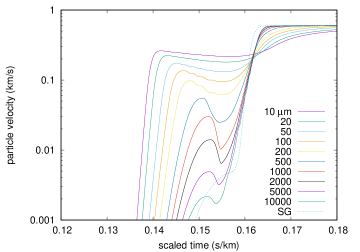
Figure 1: Particle velocity history calculated after shock wave has propagated through different thicknesses of Al using the dislocation model, compared with simulation using SG model used to calibrate $f_{b}$ assuming a strain rate of $10^{6}$/s. The drive pressure is 10 GPa in all cases. Scaled time (scaled by the propagation distance) is shown to capture the response over the wide range considered. Each trace shows an elastic precursor wave followed by plastic structure before the peak velocity is reached. The SG model is rate-independent and therefore scale-invariant. With the dislocation model, breakout of the elastic wave is earlier than with the SG model because the amplitude is much higher near the driven surface and propagates faster.

The figures below also show the SG maximum work-hardening from the $Y_{\text{max}}$ parameter, which represents the maximum yield stress reported for each metal at ambient pressure and temperature. The present dislocation model does not treat hardening as a path-dependent process as the SG model does, but we include it as an indication of the reported variation of strength with dislocation density or strain state.

Table 2: Plasticity parameters and EOS used for isentrope.

	$f_{v}$	$f_{b}$	$M$	isentrope
Al	fcc	0.096261	3.64	SESAME 3717
Cu	fcc	0.123206	3.64	SESAME 3336
Ag	fcc	0.126552	3.64	LEOS 470
Ir	fcc	0.111460	3.64	LEOS 770
Pt	fcc	0.087128	3.64	LEOS 780
Au	fcc	0.099675	3.64	LEOS 790
Pb	fcc	0.192771	3.64	LEOS 820
Fe	bcc	0.150433	3.0	SNL-SESAME 2150
Ta	bcc	0.099455	3.0	LEOS 735
W	bcc	0.125096	3.0	LEOS 740
Be	hcp	0.141415	2.0	LEOS 40
Ru	hcp	0.12	2.0	LEOS 440

IX.2 Low pressure

Considering the sensitivity to strain rate at zero pressure (Figs 2 to 4), taking $f_{b}=0.12$ gives a prediction that the fcc metals in order of increasing flow stress are Pb, Ag, Au, Cu, Pt, Al, Ir whereas the SG $Y_{0}$ order is Pb, Au, Pt, Al, Ag, Cu (no model for Ir). It is possible that the SG $Y_{0}$ may be higher than that of the pure element where impurities are common, such as Al, Cu, and Pb. The most striking outlier is Al, which is notable because $f_{b}=0.12$ appears valid for melting Swift_ajmelt_2020 . For the bcc metals, the predicted order is Fe, Ta, W, in accordance with the SG $Y_{0}$. No SG parameter set has been published for pure Fe, and the fit was performed for stainless steel. For the hcp metals considered, Be is predicted to have much lower flow stress than Ru.

For several elements, the $f_{b}=0.12$ calculation deviated from $Y_{0}$ by less than the difference between $Y_{0}$ and $Y_{\text{max}}$, which we consider encouraging performance for a parameter-free model.

For most materials starting at the lowest strain rates considered here, the flow stress is predicted to increase by roughly a factor of three per order of magnitude increase in strain rate. At sufficiently high strain rates, the sensitivity is predicted to decrease as the applied stress reduces the effective height of the Peierls barrier. This regime is reached at a lower strain rate in stronger elements, and occurs well below the theoretical maximum strength of the crystal is reached, which would be when $Y=G/2\pi$. The net effect accounts roughly for the observed difference in elastic wave amplitudes between microsecond and nanosecond scale experiments.

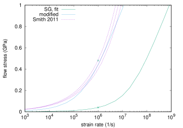
Figure 12: Predicted variation of flow stress with pressure and strain rate along the principal isentrope of Al and as deduced from rear surface velocity measurements Smith2011 .

The sensitivity of flow stress to relevant strain rates has previously been investigated in Al and Fe Smith2011 . The strain rate was estimated from the rate of acceleration of the rear surface of the sample, and it was concluded that Al exhibited effects of phonon drag for strain rates above $10^{3}$/s, whereas Fe exhibited a transition from thermal activation to phonon drag above $\sim 5\times 10^{6}$/s. The reduced data exhibited significant scatter in log space, but there are some inconsistencies in the deduced flow stress, for instance the value for Al lay well above the SG $Y_{0}$ value. Space- and time-resolved simulations of these experiments capturing the propagation and evolution of the compression wave may shed more light on the discrepancy, for example by a modified metric for strain rate and also by accounting for the evolution from initial dislocation density. For a simple comparison, we adjusted $f_{b}$ to reproduce the magnitude of the fit to the reduced data at $10^{6}$/s in Al and $5\times 10^{6}$/s in Fe: $f_{b}=$0.122261 and 0.177440 respectively. Plotting the flow stress in linear space to highlight the stiffness of the sensitivity to strain rate, the model prediction for Al reproduces the rapid increase in flow stress with strain rate without requiring an explicit phonon drag term (Fig. 12). The prediction for Fe did not exhibit the same degree of stiffening. As well as the same caveats about resolving the propagating waves and accounting for the evolving dislocation density, additional complexities for Fe include the impedance mismatch with the transparent window and phase transformations which occurred during the laser-driven experiments and could affect the driving stress.

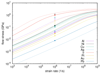
Figure 2: Flow stress for face-centered cubic elements at zero pressure, predicted with $f_{b}=0.12$ (dashed) and with $f_{b}$ fitted to SG $Y_{0}$ (solid). Circles show $Y_{0}$ (filled) and $Y_{\text{max}}$ (open) where available, in the same color as the corresponding line.

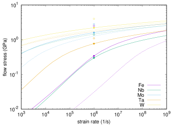
Figure 3: Flow stress for body-centered cubic elements at zero pressure, predicted with $f_{b}=0.12$ (dashed) and with $f_{b}$ fitted to SG $Y_{0}$ (solid). Circles show $Y_{0}$ (filled) and $Y_{\text{max}}$ (open) where available, in the same color as the corresponding line.

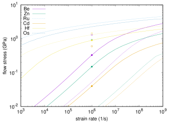
Figure 4: Flow stress for hexagonal close-packed elements at zero pressure, predicted with $f_{b}=0.12$ (dashed) and with $f_{b}$ fitted to SG $Y_{0}$ (solid). Circles show $Y_{0}$ (filled) and $Y_{\text{max}}$ (open) where available, in the same color as the corresponding line.

IX.3 High pressure

We consider the variation of flow stress with pressure along the principal isentrope, for simplicity in the graphs below neglecting the temperature increase from plastic work, which is a small correction on the scale of these graphs. We consider only the fitted value of $f_{b}$ as for most of these metals $f_{b}=0.12$ did not reproduce the SG $Y_{0}$ adequately. Atom-in-jellium EOS are often inaccurate at pressures below a few tenths of a terapascal, so we took the principal isentropes from semi-empirical wide-range EOS libraries sesame ; leos , as listed in Table 2. To emphasize, the plasticity model above is defined in terms of $\rho$, $T$, $\epsilon_{e}$, and $\phi_{d}$: it does not depend explicitly on pressure, and so the choice of EOS is not an inherent part of the model. (The shear modulus and Einstein temperature should in principle be consistent with the EOS, and the Peierls barrier is also related to the EOS though less directly.)

As well as the predictions of the present model, we also show the yield stress calculated using the SG model along the same isentrope. To span all possible loading paths, we plot curves for both $Y_{0}$ and $Y_{\text{max}}$, i.e. the least and greatest contribution possible from work-hardening according to that model.

Considering the behavior in more detail for representative elements (Figs 5 to 11), those of lower $Z$ such as Be are predicted to retain a large dependence of flow stress on strain rate to high pressures. For fcc elements of moderate to high $Z$, the sensitivity of flow stress to strain rate is large at low pressures but decreases at pressures above $\sim 100$ GPa. For bcc elements of moderate to high $Z$, the sensitivity of flow stress to strain rate is less than that of fcc elements at low pressure, but decreases more slowly with pressure. For Ta in particular, the flow stress at pressures of a few hundred gigapascals and a strain rate $10^{7}$/s representative of Rayleigh-Taylor ripple growth experiments is close to twice the SG $Y_{\text{max}}$ value. The flow stress of metals including Ta and Au has been estimated at pressures $\sim 0.1$ TPa from release features in the velocity history transmitted through ramp-loaded samples Brown2021 . The strain rate in these experiments was nominally $5\times 10^{5}$/s, but it was likely somewhat lower at low pressures and higher at high pressures, and we suggest that the measurements likely sampled a range $10^{5}-10^{6}$/s. This is a recent experimental development and the uncertainties are relatively large, but the trend and magnitude appear consistent with our predictions. A recent study Prime2022 found that previous multi-scale plasticity models and models constructed using more detailed dislocation processes do not accurately predict the flow stress at pressures above $\sim$0.1 TPa, and require further study. Specifically, the models evaluated for Ta were not consistent with experimental measurements at higher pressure unless recalibrated to match. It is striking that the present theory predicts flow stresses consistent with the measurements when calibrated to a single, low-pressure datum. Either the dominant mechanisms of plastic flow do not change between the fitting and test states, or any competing mechanism fortuitously exhibits the same dependencies.

The contribution of the core and strain energy of the dislocations is predicted to be significant. At low pressures, calculated as above, it can easily exceed the pressure from the EOS. This is misleading, because we are concerned with near-uniaxial loading, and it is not possible to sustain the strain rate for long enough to build up an equilibrium population of dislocations before the pressure rises substantially. However, for pressures into the terapascal range, the dislocation pressure tends toward a few percent of the mean pressure, which may be a significant correction when interpreting dynamic loading behaviour in terms of the scalar EOS.

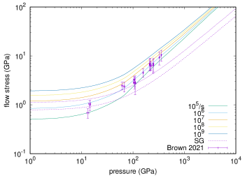
Figure 5: Predicted variation of flow stress with pressure and strain rate along the principal isentrope of Ta, $f_{b}$ fitted to SG $Y_{0}$. Magenta lines: SG $Y_{0}$ (lower) and $Y_{\text{max}}$ (upper), with predicted dependence on pressure and temperature along the isentrope. Brown data were nominally at $5\times 10^{5}$/s.

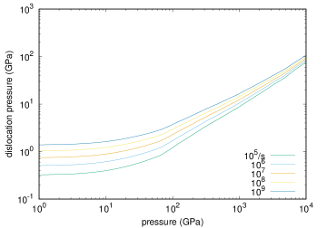
Figure 6: Predicted variation of dislocation pressure with pressure and strain rate along the principal isentrope of Ta, $f_{b}$ fitted to SG $Y_{0}$.

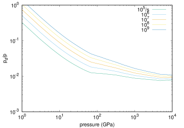
Figure 7: Predicted ratio of dislocation pressure $p_{d}$ to pressure $p$ along the principal isentrope of Ta, $f_{b}$ fitted to SG $Y_{0}$.

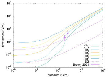
Figure 8: Predicted variation of flow stress with pressure and strain rate along the principal isentrope of Au, $f_{b}$ fitted to SG $Y_{0}$. Magenta lines: SG $Y_{0}$ (lower) and $Y_{\text{max}}$ (upper), with predicted dependence on pressure and temperature along the isentrope. Brown data were nominally at $5\times 10^{5}$/s.

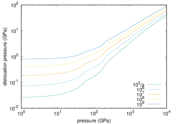
Figure 9: Predicted variation of dislocation pressure with pressure and strain rate along the principal isentrope of Au, $f_{b}$ fitted to SG $Y_{0}$.

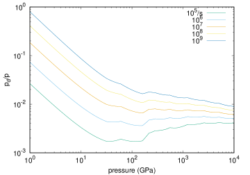
Figure 10: Predicted ratio of dislocation pressure $p_{d}$ to pressure $p$ along the principal isentrope of Au, $f_{b}$ fitted to SG $Y_{0}$.

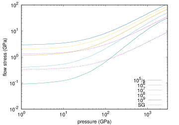
Figure 11: Predicted variation of flow stress with pressure and strain rate along the principal isentrope of Be, $f_{b}$ fitted to SG $Y_{0}$. Magenta lines: SG $Y_{0}$ (lower) and $Y_{\text{max}}$ (upper), with predicted dependence on pressure and temperature along the isentrope.

X Conclusions

We describe a continuum-level plasticity model for polycrystalline materials based on a single dislocation density and single mobility mechanism, with an evolution model for the dislocation density. Using the approximate but wide-ranging and computationally efficient atom-in-jellium model for the electronic structure of matter to predict the shear modulus, Einstein frequency, and systematic variation of the Peierls barrier, we deduce a credible variation of flow stress with pressure and strain rate. In this formulation, the equilibrium dislocation density is an emergent property of the model. With the dislocation density expressed per-atom rather than as a dislocation length per volume, to simplify the plasticity relations at finite compressions, its value was predicted to vary less with pressure. Interestingly, stiffening at high strain rates that is usually attributed to phonon drag may be accounted for by the form of the hopping rate.

The model is constructed to make it straightforward to substitute alternative forms for key components, such as the shear modulus, hopping attempt rate, Peierls barrier, and terms in the dislocation evolution equation, where more accurate relations are available. It may also be possible to generalize the dislocation mobility to account for several types of barrier, represented with a rheonet.

In estimating the Peierls barrier from the Einstein frequency, we find a potential link to the Lindemann melting law, which leads to a parameter-free approximate plasticity model. This approach otherwise requires a single free parameter to be determined from experiment or more detailed theory.

Accounting for the elastic energy of the dislocations gives a prediction of the plastic work appearing as heat, equivalent to a dynamic, self-consistent estimate of the Taylor-Quinney factor, which has long been a poorly-constrained parameter or assumption in simulations of plastic flow. The elastic energy of the dislocations is predicted to be manifested also as a contribution to the pressure, which may reach several percent of the total pressure in ramp compression to the terapascal range, and should therefore be considered when interpreting ramp data as an isentrope or isotherm. The bulk elastic shear energy also contributes to the pressure, but is much smaller. The mean pressure is usually assumed to depend only on the scalar equation of state and not in general on the elasticity or strength: both of these contributions represent new physics at high dynamic pressures. We also find that a constant shear modulus would lead to a negative contribution to pressure from both elastic shear and dislocation energies, which may not have been previously appreciated.

The model reproduces the observation that the elastic wave amplitude for loading of samples $o(10)$ $\mu$m thick, on nanosecond time scales, corresponds to a flow stress a few times higher than for samples $o(10)$ mm thick, on microsecond time scales. It predicts a reduced dependence of flow stress on strain rate in higher-$Z$ materials, particularly in the face-centered cubic structure, at pressures over $\sim 100$ GPa. The predictions are reasonably consistent with recent assessments of strength at high pressure from surface velocimetry data, whereas other known plasticity models were not consistent without calibration to the data.

Appendix A: Pressure contributions

The contributions to specific energy of the material from the dislocation population and from the bulk elastic shear strain take the form

$$e\propto G/\rho=\alpha G/\rho\text{, say}.$$ (32)

Pressure depends on the Helmholtz specific free energy $f$ as $p=-\partial f/\partial v|_{T}$ where $v$ is the specific volume, $1/\rho$, so

$$p=\rho^{2}\left.\frac{df}{d\rho}\right|_{T}.$$ (33)

As usual for EOS construction, we assume that contributions to free energy are additive, which means that the corresponding contributions to pressure can be also considered separately and added. The shear modulus $G$ varies in principle with $\rho$ and $T$. Its temperature variation subsumes the implicit entropy dependence of $G$. If we neglect any explicit entropy dependence of these contributions to the specific energy then $f=e$, which is equivalent to assessing the pressure contributions along the cold compression curve. Differentiating,

$$p=\alpha\left(\rho\left.\frac{dG}{d\rho}\right|_{T}-G\right).$$ (34)

Factorizing out $G$ and noting that $\alpha G=\rho e$ by Eq. 32, we find that the pressure contribution can be expressed with respect to the dimensionless logarithmic derivative of $G$ with respect to $\rho$:

$$p=\rho e\left(\frac{\rho}{G}\left.\frac{\partial G}{\partial\rho}\right|_{T}-1\right).$$ (35)

This derivation implies that a constant shear modulus leads to negative pressure contributions from the dislocations and shear strain, which may seem surprising. However, it follows by inspection from Eq. 32: increasing $\rho$ at constant $G$ leads to a decrease in specific energy, and thus leads to a tensile contribution to pressure. If we consider a power-law dependence $G\propto\rho^{\beta}$ then

$$p=\rho e(\beta-1).$$ (36)

Thus, in order for these pressure contributions to be positive, the effective exponent for the dependence of $G$ on $\rho$ must exceed unity.

Appendix B: Deviatoric elastic strain

The contribution of deviatoric elastic strain to pressure is a minor part of the results reported, but caused some discussion during manuscript review.

Studies of quasistatic loading often employ high-order elasticity, which expresses the components of the stress tensor as a Taylor expansion about the initial state. Third-order components can capture a connection between shear and pressure, and this has been recognized in low-symmetry crystal structures at low pressure and also in soft materials exhibiting large elastic strains, such as rubbers.

The analysis presented here implies that elastic shear in a material described even by only second-order deviatoric elastic moduli results in a contribution to pressure, depending on the variation of the moduli with compression. This result has been deduced previously in a similar though not identical form, following a longer derivation Scheidler1996 which also considers the effect of third-order contributions. The previous analysis is equivalent to ours, but there is an error in the associated discussion that may have caused readers some confusion: Eq. 4.7 in the report reads

$$p_{2}>0\iff\tilde{\rho}\frac{d\mu}{d\tilde{\rho}}>\mu\iff\frac{d\mu}{d\tilde{p}}>\frac{\mu}{\kappa}\iff\frac{dU_{s}}{d\tilde{p}}>0$$

where $p_{2}$ is the contribution to isotropic pressure $\tilde{p}$, $\tilde{\rho}$ is the compression ratio with respect to the initial state $=\rho/\rho_{0}$, $\mu$ is the shear modulus, $\kappa$ the bulk modulus, and $U_{s}$ the shear wave speed. The inequalities are equivalent to testing $(\rho/G)\partial G/\partial\rho>1$ in our Eq. 24. In the discussion immediately following Eq. 4.7, the report states “$dU_{s}/d\tilde{p}$ implies $d\mu/d\tilde{p}>0$” which is inconsistent with Eq. 4.7 and with our derivation, though the report goes on to use Eq. 4.7 consistently to evaluate pressure-shear coupling at ambient conditions in seven materials including four elemental metals. It seems possible that an error such as this may have led to the misconception that a constant shear modulus leads to no pressure-shear coupling, as this report has been cited in publications in this area.

Pressure-shear coupling has been linked with anisotropy Fuller2011 in a literature that indicates that such phenomena are recognized for geologic materials and ceramics, but not for metals because elastic strains tend to be too small for anisotropic effects to become significant or do not occur in cubic crystals. This narrative is consistent with our work, because dynamic loading under HED conditions can induce high compressions at relatively low temperatures, on time scales where the elastic strain may be much larger than customary and thus potentially important to account for. It has also been suggested that pressure-shear coupling can only occur in non-cubic crystals Luscher2017 . However, pressure-shear coupling in our analysis and that of Scheidler1996 may occur from purely isotropic deviatoric elasticity, and may occur in cubic crystals, although of course they cease to be cubic when deformed.

Pressure-shear coupling can also be captured in high-order elasticity theory, in which the stress tensor is expressed as a Taylor series with respect to elastic strains from a reference state, usually the initial, undeformed state. Pressure-shear contributions can occur from third-order and higher terms, in contrast to the contribution from second-order deviatoric elasticity that occurs here via the compression dependence of the shear modulus. Although dislocation plasticity models have been constructed on higher-order elasticity theory Nguyen2021 , this formalism is not an appropriate over the range of pressures of interest to us. Matter may exhibit orders of magnitude of isotropic compression, whereas the maximum elastic shear strain possible is a few tens of percent (depending on on crystal structure and shear orientation) before the shear stress decreases by symmetry of the lattice. Therefore, a Taylor expansion in strain from the initial state is less appropriate than a strain-invariant isotropic model such as a scalar EOS, supplemented by a Taylor expansion about the state of isotropic stress.

References

- (1) C.J. Horowitz and K. Kadau, Phys. Rev. Lett. 102, 191102 (2009).
- (2) P. Campbell, M. Hill, R. Howe, J.F. Kielkopf, N. Lewis, J. Mandaville, A. McWilliams, W. Moos, D. Samouce, J. Winkler, G.J. Fishman, A. Price, D.L. Welch, P. Schnoor, A. Clerkin, and D. Saum, Gamma-ray Coordinates Network (GCN) Gamma Ray Burst (GRB) Observation report 2932, Am. Assoc. Variable Star Observers, aavso.org and https://gcn.gsfc.nasa.gov (2005).
- (3) For example, H.-S. Park, K.T. Lorenz, R.M. Cavallo, S.M. Pollaine, S.T. Prisbrey, R.E. Rudd, R.C. Becker, J.V. Bernier, and B.A. Remington, Phys. Rev. Lett. 104, 135504 (2010); R. Rygg, R.F. Smith, A.E. Lazicki, D.G. Braun, D.E. Fratanduono, R.G. Kraus, J.M. McNaney, D.C. Swift, C.E. Wehrenberg, F. Coppari, M.F. Ahmed, M.A. Barrios, K.J.M. Blobaum, G.W. Collins, A.L. Cook, P. Di Nicola, E.G. Dzenitis, S. Gonzales, B.F. Heidl, M. Hohenberger, A.House, N. Izumi, D.H. Kalantar, S.F. Khan, T.R. Kohut, C. Kumar, N.D. Masters, D.N. Polsin, S.P. Regan, C.A. Smith, R.M. Vignes, M.A. Wall, J. Ward, J.S. Wark, T.L. Zobrist, A. Arsenlis, and J.H. Eggert, Rev. Sci. Instrum. 91, 043902 (2020).
- (4) J. Lindl, Phys. Plasmas 2, 3933 (1995).
- (5) N.R. Barton, J.V. Bernier, R. Becker, A. Arsenlis, R. Cavallo, J. Marian, M. Rhee, H.-S. Park, B.A. Remington, and R.T. Olson, J. Appl. Phys. 109, 073501 (2011).
- (6) N.R. Barton and M.R. Rhee, J. Appl. Phys. 114, 123507 (2013).
- (7) J.J. Mason, A.J. Rosakis and G. Ravichandran, Mech. Materials 17, 135-145 (1994).
- (8) R. Kapoor and S. Nemat-Nasser, Mech. Materials 27, 1-12 (1998).
- (9) P. Rosakis, A.J. Rosakis, G. Ravichandran, and J. Hodowany, J. Mech. Phys. Solids 48, 581-607 (2000).
- (10) J. Hodowany, G. Ravichandran, A.J. Rosakis, and P. Rosakis, Exp. Mech. 40, 2, 113-123 (2000).
- (11) A. Zubelewicz, Phys. Rev. B 77, 214111 (2008).
- (12) A. Zubelewicz, Sci. Rep. 9, 9088 (2019).
- (13) D.C. Swift, T. Lockard, M. Bethkenhagen, R.G. Kraus, L.X. Benedict, P. Sterne, M. Bethkenhagen, S. Hamel, and B.I. Bennett, Phys. Rev. E 99, 063210 (2019).
- (14) D.C. Swift, T. Lockard, S. Hamel, C.J. Wu, L.X. Benedict, P.A. Sterne, and H.D. Whitley, arXiv:2103.03371 (2021).
- (15) D.C. Swift, T. Lockard, M. Bethkenhagen, S. Hamel, A. Correa, L.X. Benedict, P.A. Sterne, and B.I. Bennett, Phys. Rev. E 101, 053201 (2020).
- (16) D.C. Swift, T. Lockard, S. Hamel, C.J. Wu, L.X. Benedict, and P.A. Sterne, Phys. Rev. B 105, 024110 (2022).
- (17) D.C. Swift, E.N. Loomis, P. Peralta, and B. El-Dasher, arXiv:0801.0271 (2008).
- (18) D.L. Preston, D.L. Tonks, and D.C. Wallace, J. Appl, Phys. 93, 211 (2003).
- (19) R.A. Austin, J. Appl. Phys. 123, 035103 (2018).
- (20) C.S. Deo, D.J. Srolovitz, W. Cai, and V.V. Bulatov, J. Mech. Phys. Solids 53, 1223-1247 (2005).
- (21) F.A. Nichols, Mater. Sci. Eng. 8, pp 108-120 (1971).
- (22) R.M.J. Cotterill, Phys. Lett. A 60, 61–62 (1977).
- (23) E.O. Hall, Proc. Phys. Soc. Lond. 64, 9, 747–753 (1951).
- (24) N.J. Petch, J. Iron Steel Inst. London. 173, 25–28 (1953).
- (25) P.A.M. Dirac, “Approximate Rate of Neutron Multiplication for a Solid of Arbitrary Shape and Uniform Density,” British Report MS-D-5, Part I. (1943); in R.H. Dalitz (Ed.),“The Collected Works of P. A. M. Dirac 1924–1948,” pp 1115–1128 (Oxford University Press, Oxford, 1995).
- (26) W.S. Farren and G.I. Taylor, Proc. Roy. Soc. A107, 422 (1925).
- (27) G.I. Taylor and H. Quinney, Proc. Roy. Soc. A143, 307 (1934).
- (28) J.C. Stimac, N. Bertin, J.K. Mason, and V.V. Bulatov, arXiv:2205.04653 (2022).
- (29) L.A. Zepeda-Ruiz, A. Stukowski, T. Oppelstrup, and V.V. Bulatov, Nature 550, 492 (2017).
- (30) V. Bulatov (Lawrence Livermore National Laboratory), private communication (2021).
- (31) D.C. Swift and G.J. Ackland, Appl. Phys. Lett. 83, 1151 (2003).
- (32) G.I. Taylor, Proc. Roy. Soc. A145, 362 (1934).
- (33) D.C. Swift, T. Lockard, R.F. Smith, C.J. Wu, and L.X. Benedict, Phys. Rev. Research 2, 023034 (2020).
- (34) F.D. Stacey and R.D. Irvine, Aust. J. Phys. 30, 641-646 (1977).
- (35) L. Burakovsky, D.L. Preston, and R.R. Silbar, Phys. Rev. B 61, 22, 15011 (2000).
- (36) T. Lockard et al, in preparation.
- (37) K. Alidoost et al, in preparation.
- (38) H.-S. Park, K.T. Lorenz, R.M. Cavallo, S.M. Pollaine, S.T. Prisbrey, R.E. Rudd, R.C. Becker, J.V. Bernier, and B.A. Remington, Phys. Rev. Lett. 104, 135504 (2010).
- (39) M.W. Guinan and D. Steinberg, J. Phys. Chem. Solids 35, 1501 (1974).
- (40) D.J. Steinberg, S.G. Cochran, and M.W. Guinan, J. Appl. Phys. 51 (3), 1498-1504 (1980).
- (41) D.J. Steinberg, Lawrence Livermore National Laboratory report UCRL-MA-106439 change 1 (1993).
- (42) S.P. Lyon and J.D. Johnson, Los Alamos National Laboratory report LA-UR-92-3407 (1992).
- (43) D.A. Young and E.M. Corey, J. Appl. Phys. 78, 3748 (1995).
- (44) B. Goldstein (DERA Fort Halstead), private communication (1993).
- (45) S.G. Srinivasan, M.I. Baskes, and G.J. Wagner, J. Mat. Sci. 41, 23, 7838-7842 (2006).
- (46) R.E. Rudd (Lawrence Livermore National Laboratory), unpublished.
- (47) J.L. Brown, J.‐P. Davis, and C.T. Seagle, J. Dyn. Behavior Mat. 7, 196-206 (2021).
- (48) R.F. Smith, J.H. Eggert, R.E. Rudd, D.C. Swift, C.A. Bolme, and G.W. Collins, J. Appl. Phys. 110, 123515 (2011).
- (49) M. Scheidler, On the coupling of pressure and deviatoric stress in isotropic hyperelastic materials, Army Research Laboratory report ARL-TR-954 (1996).
- (50) T. Fuller and R.M. Brannon, Int. J. Eng. Sci. 49, 311-321 (2011).
- (51) D.J. Benson, Comp. Meth. App. Mech. Eng. 99, 2-3, 235-394 (1992).
- (52) J.A. Rodríguez-Martínez, M. Rodríguez-Millán, A. Rusinek, and A. Arias, Mech. Mat. 43, 901 (2011).
- (53) C.Y. Gao and L.C. Zhang, Int. J. Plasticity 32, 121 (2012).
- (54) H. Lim, C.C. Battaile, J.D. Carroll, B.L. Boyce, and C.R. Weinberger, J. Mech. Phys. Solids 74, 80-96 (2015).
- (55) A. Hunter and D.L. Preston, Int. J. Plasticity 70, 1 (2015).
- (56) A. Hunter and D.L. Preston, Int. J. Plasticity 151, 103178 (2022).
- (57) D.N. Blaschke, A. Hunter, and D.L. Preston, Int. J. Plasticity 131, 102750 (2020).
- (58) P.G. Heighway, M. Sliwa, D. McGonegle, C. Wehrenberg, C.A. Bolme, J. Eggert, A. Higginbotham, A. Lazicki, H.-J. Lee, B. Nagler, H.-S. Park, R.E. Rudd, R.F. Smith, M.J. Suggit, D. Swift, F. Tavella, B.A. Remington, and J.S. Wark, Phys. Rev. Lett. 123, 245501 (2019).
- (59) C.K.C. Lieou and C.A. Bronkhorst, Acta Mat. 202, 170 (2021).
- (60) G.C. Soares and M. Hokka, Int. J. Impact Eng. 156, 103940 (2021).
- (61) M.B. Prime, A. Arsenlis, R.A. Austin, N.R. Barton, C.C. Battaile, J.L. Brown, L. Burakovsky, W.T. Buttler, S.-R. Chen, D.M. Dattelbaum, S.J. Fensin, D.G. Flicker, G.T. Gray III, C. Greeff, D.R. Jones, J.M.D. Lane, H. Lim, D.J. Luscher, T.R. Mattsson, J.M. McNaney, H.-S. Park, P.D. Powell, S.T. Prisbrey, B.A. Remington, R.E. Rudd , S.K. Sjue, and D.C. Swift, Acta Mat. 231, 117875 (2022).
- (62) For example, D.J. Luscher, F.L. Addessio, M.J. Cawkwell, and K.J. Ramos, J. Mech. Phys. Solids 98, 63-86 (2017).
- (63) For example, T. Nguyen, S.J. Fensin, and D.J. Luscher, Int. J. Plasticity 139, 102940 (2021).
- (64) D.C. Swift, Lawrence Livermore National Laboratory report LLNL-MI-831439 (2022); https://gdo-hdp.llnl.gov/matprops/aj/disloc2021/