AC sensing using nitrogen vacancy centers in a diamond anvil cell up to 6 GPa

Abstract

Nitrogen-vacancy color centers in diamond have attracted broad attention as quantum sensors for both static and dynamic magnetic, electrical, strain and thermal fields, and are particularly attractive for quantum sensing under pressure in diamond anvil cells. Optically-based nuclear magnetic resonance may be possible at pressures greater than a few GPa, and offers an attractive alternative to conventional Faraday-induction based detection. Here we present AC sensing results and demonstrate synchronized readout up to 6 GPa, but find that the sensitivity is reduced due to inhomogeneities of the microwave field and pressure within the sample space. These experiments enable the possibility for all-optical high resolution magnetic resonance of nanoliter sample volumes at high pressures.

I Introduction

Nuclear magnetic resonance is one of the most versatile tools for investigating condensed matter in extreme conditions, including temperatures ranging from sub-mK to 1000 K, static magnetic fields up to 45 T, pulsed magnetic fields [1], uniaxial strain, and hydrostatic pressures up to several GPa [2]. Each of these environments presents special challenges for conducting magnetic resonance experiments, but pressure is exceptional because of the small volumes available. The maximum achievable pressure in of a given pressure cell scales roughly as the inverse of the sample volume, and depends on the material parameters and design of the cell. Intermediate-scale pressures up to 2-3 GPa can be reached within a piston-cylinder type cell, with volumes on the order of several hundred $\mu$L. For this type of pressure cell, it is straightforward to introduce a small coil and perform conventional NMR. This approach has become standard in the study of condensed matter systems [3] as well as solution chemistry at high pressure [4].

Figure 1: Diamond anvil cell for optically-detected magnetic resonance experiments. An objective focuses the excitation light and collects the fluorescence from within the sample space in the gasket. A straight gold antenna is located across the anvil culet ( sample hole 260 $\mu$m diameter), and a small NV diamond crystal of dimensions $\sim 100\times 75$ $\mu$m is visible at the center to the lower right of the antenna (see arrow), oriented normal the [100] direction. A magnetic field of magnitude $H_{0}\sim 10$ mT is oriented $54.7^{\circ}$ from the vertical along the [111] direction of the diamond using permanent neodymium magnets mounted externally.

Piston-cylinder type cells are limited to approximately 2-3 GPa due to the Young’s modulus of the Cu-Be alloy that forms the cylinder housing [5]. Alternative designs can extend this pressure range up to 4.5 GPa [6], although with severe constraints on the sample volume. To reach pressures beyond this range, it is necessary to use a diamond anvil cell(DAC), in which a pair of diamond anvils compress a sample volume contained within a metallic gasket, as illustrated in Fig. 1 [7]. The available sample volume is only on the order of 0.1-1 nL, presenting serious challenges for conventional NMR. Not only should a solenoid be located within this space to form a high $Q$ resonant circuit and introduce the necessary radiofrequency fields for NMR, but the leads must also be insulated from the gasket. Preventing leads from shorting or breaking under pressure is a major challenge [8]. Secondly, the nuclear magnetization needs to be large enough to induce a sufficient voltage relative to the Johnson noise of the coil. Typically this requires on the order of $10^{17}$ nuclear spins [9]. For a typical solid, e.g. copper with density 10 g/cm³, this limit corresponds to 1 nL. Since the sample space must also contain the coil and pressure medium, there is often insufficient room for the minimum detectable sample. Although there have been recent advances to overcome these limitations using specialized microcoils, gasket resonators and Lenz lenses enabling NMR measurements up to the hundred GPa regime [10, 2, 11], alternative detection methods may be advantageous in order to investigate matter at higher pressures, for example superconductivity in hydride compounds(hydrogen-rich materials) [12, 13, 14].

Optically-detected magnetic resonance (ODMR) of NV centers offers an alternative and complementary approach that is not limited by the small sample volume and can detect nuclear spins within volumes as small as $10^{-3}$ nL with sub-mHz resolution. Several excellent reviews are available outlining the basics of this technique [15, 16, 17]. The fluorescence intensity of the NV centers is a strong function of the NV spin ($S=1$) orientation, and the NV centers can be optically pumped to the ground state with high polarization. Single NV detection is possible with polarization $>99\%$ using optical pumping resonant with the zero-phonon line [18]. For NV ensembles with non-resonant pumping using 532 nm light, the optical contrast is a few percent. Because detection is optical-based rather than using Faraday induction, it is no longer necessary to locate a high Q resonant circuit within the sample space. The spin orientation can be measured optically, in which excitation and fluorescence light passes through the transparent diamond anvils and can be focused down to a point on the sample of size $\sim 1\mu$m, enabling work with small samples. ODMR has been utilized to study static strain and magnetization as a function of pressure and temperature [19, 20, 21, 22]. Here we describe AC sensing experiments using NV centers in a diamond anvil cell to probe dynamic fields, such as those arising from precessing nuclear spins. In principle there is no upper limit for such measurements, and we discuss some of the challenges that emerge under pressure as the properties of the NV centers evolve.

II Apparatus

The principle challenges to performing ODMR in a DAC are associated with the collecting sufficient fluorescence from the sample as well as introducing microwaves with sufficient homogeneity and magnitude. Fortunately, ODMR is similar in practice to Raman spectroscopy, which is a well-established technique under pressure in DACs.

Figure 2: (Left) Rabi frequency of the $|0\rangle\leftrightarrow|-1\rangle$ transition and (Right) fluorescence intensity measured as a function of position in an diamond crystal with NV centers located within a DAC. The scanning step size is 20 $\mu$m, or the scale of the individual squares on the map.

II.1 Design and Microwave Antenna

Compared to ambient conditions, the signal-to-noise for ODMR in a DAC will be reduced because the structure of the cell prevents the objective from being too close to the sample. For our design, illustrated in Fig. 1, the distance to the diamond anvil is approximately 10 mm, plus 2.5 mm for the the anvil itself. It is thus necessary to utilize a long-working distance objective (Nikon CFI T Plan Epi SLWD 50X Objective, N.A. 0.40 and working distance 22 mm). The pressure cell (CryoDAC SC, Almax-Easylab), is mounted on a translation stage and an external magnetic field, $\mathbf{H}_{0}$, of 29 mT oriented at an angle of 54.7^∘ from the vertical is introduced via a pair of fixed neodynium permanent magnets. The gaskets are fabricated with 0.3 mm thick copper-beryllium, and the sample holes of diameter of 260 $\mu$m are drilled through the center of the pre-indented region (depth ranges from 100 to 150 $\mu$m) using an electrical discharge machine. A small diamond crystal prepared with 0.3 ppm NVs (Element 6) was cut and polished to a thickness of 20 $\mu$m (Applied Diamond/Diamond Delaware Knives), and then secured to the anvil with superglue such that the $[100]$ axis is aligned parallel to the DAC axis. The ODMR spectrum is measured as the cell is rotated along the DAC axis in order to align the field along the $[111]$ direction parallel to the NV axis. The diamond anvils are type IIac with low nitrogen impurities in order to minimize background fluorescence. The spot size of the laser is less than 20 $\mu$m, and can be scanned laterally across the sample space. Representative scans of the Rabi frequency, $\Omega$, and fluorescence intensity are shown in Fig. 2.

Introducing microwaves with sufficient magnitude in close proximity to the NV centers presents a major challenge for working in a DAC, because the conducting gasket can screen out the magnetic field, as illustrated in Fig. 3. High microwave amplitudes are necessary in order to achieve strong $\mathbf{H}_{1}$ fields and hence large Rabi frequencies. The magnitude of $\mathbf{H}_{1}$ should be $\sim 0.18$ mT in order to have a 90^∘ pulse time on the order of 50 ns ( $\Omega\sim 5$ MHz). Note that it is not necessary to have a high $Q$ resonant circuit, so the antenna does not necessarily need to have a low resistance. Previous studies have utilized antennas located external to the sample chamber [23, 19, 20, 22], within the sample chamber [21], as well as designer anvils with conducting paths deposited directly onto the diamond culet and protected with a capping layer of CVD grown diamond [24]. Locating the antenna outside the sample space, as shown in Fig. 3(a,b), is easier, but is inefficient because a large fraction of the power goes towards inducing screening currents in the conducting gasket and can lead to undesired heating effects. Designer anvils are costly and time consuming to prepare [25].

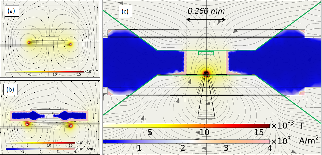
Figure 3: Calculated magnetic field profile from a wire loop surrounding a diamond anvil close to (a) an insulating gasket and (b) a conducting gasket for 63.2 V(40 dBm) across the antenna at 3 GHz. The conducting gasket screens the majority of the magnetic field within the sample space. (c) The calculated magnetic field profile and induced current density for a conducting gasket with a straight antenna, as illustrated in Fig. 4(a). The diamond anvil (outlined in green) has a relative permeability of 5 [26]. The green rectangle in the sample space represents the volume of the NV diamond chip used to compute the histograms in Fig. 5.

To overcome this challenge, we fabricated gold microwave strips, as shown in Fig. 4, by electroplating 8 $\mu$m thick strips onto a substrate, which were then liberated chemically for insertion into the DAC. A single antenna is then transferred onto the culet of the anvil with tweezers under a microscope, and secured with thin layer of adhesive. Leads were attached to the ends of the antenna pads with silver epoxy, and then attached to larger wires (not shown) that lead out of the cell and to a high power (16 W) microwave amplifier (Mini-Circuits, ZHL-16W-43-S+). The antenna is insulated from the pre-indented region of the gasket with a mixture of epoxy and aluminum oxide and(or) boron nitride powders, that are cured under compression (Fig. 4(c)). After the epoxy has cured, the center hole is drilled out, leaving a thin layer of insulating material between the conducting gasket and the antenna leads [27]. This approach enables us to reliably apply pressure to the gasket without comprising the antenna performance. The antenna leads are malleable and are compressed under pressure as the anvil presses into the gasket. However, at higher pressures (on the order of $\sim 10-30$ GPa) the leads will eventually sever as the gasket deforms and the anvil cups inward [28]. In such cases it may be better to utilize alternative designs, with thinner leads or even eliminating the leads altogether and using the Lenz lens approach of Ref. [28] For pressures up to $\sim 7$ GPa we can achieve Rabi frequencies of several tens of MHz with our antenna, which correspond to $90^{\circ}$ pulses of a few tens of nanoseconds, as illustrated in Fig. 5. Eventually for sufficiently high pressure the antenna leads are thinned out and clipped by the anvils, limiting the power delivered and dramatically decreasing the Rabi frequency. Microwaves pulse sequences are generated via an arbitrary waveform generator (Tabor AWG Model SE5082).

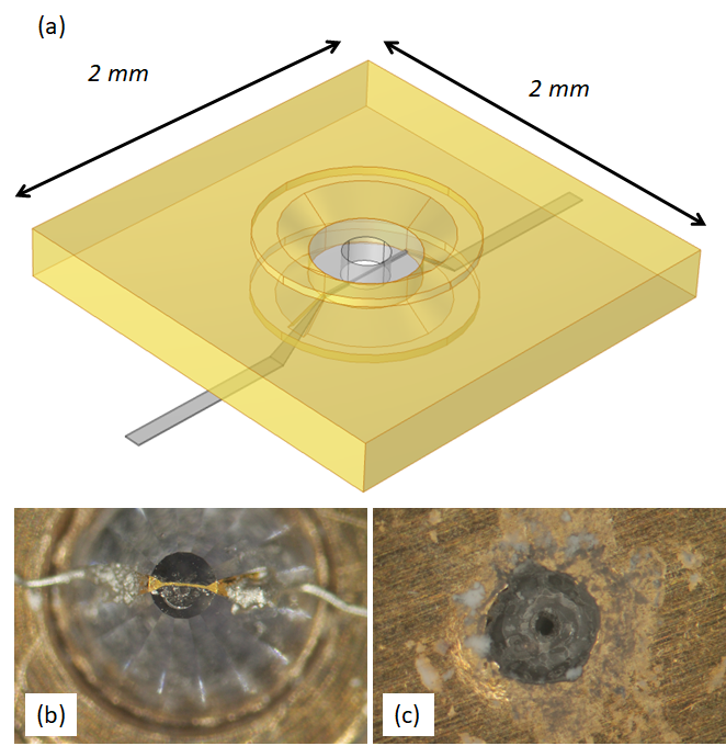
Figure 4: (a) Geometry of the gasket and sample region. The inner diameter is 260 $\mu$m, the culet diameter is 600 $\mu$m, and the thickness of the sample region is 150 $\mu$m. The gasket is copper-beryllium with conductivity 1.16$\times 10^{7}$ S/m. The gold antenna has width 11$\mu$m, thickness 8 $\mu$m and length 600 $\mu$m, and has conductivity 4.6$\times 10^{7}$ S/m. There is also a thin insulating layer between the antenna and gasket with conductivity $10^{-18}$ S/m. (b) Fabricated microwave antenna secured onto culet of the anvil (diameter 600 $\mu$m). The antenna has width 10 $\mu$m and thickness 8 $\mu$m. (c) Pre-indented gasket with insulating layer of boronitride, aluminum oxide and epoxy. The sample space in the center hole has diameter 260 $\mu$m.

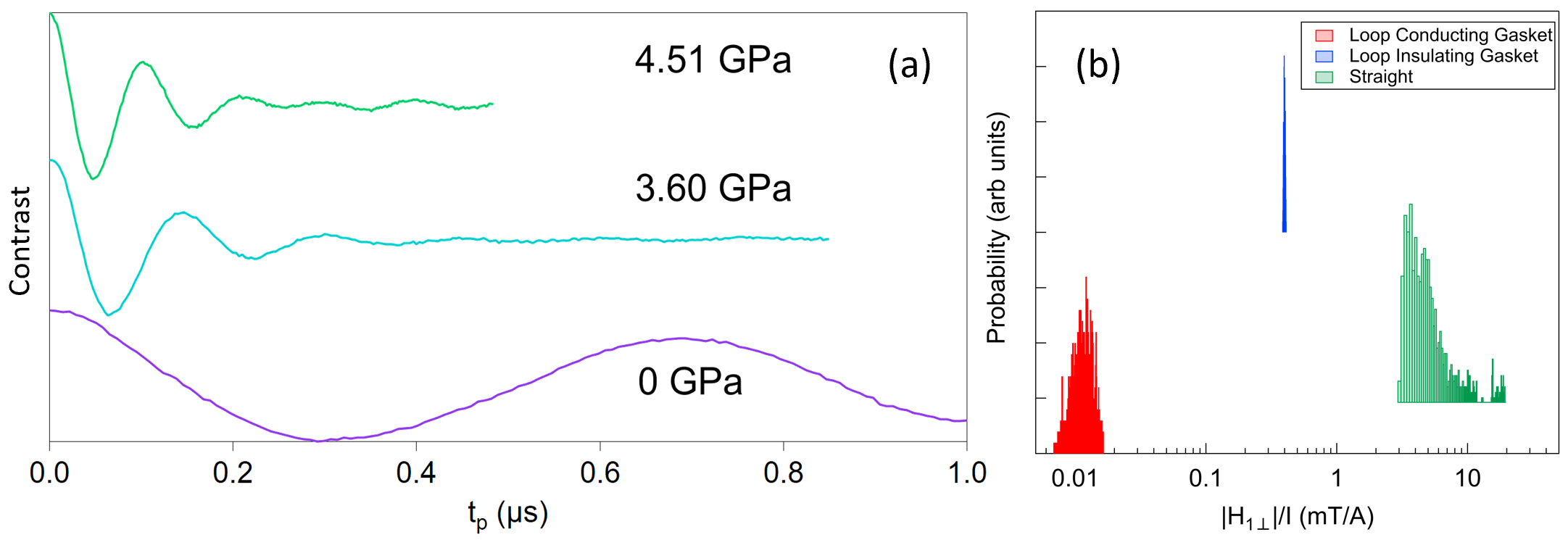
Figure 5: (a) Rabi oscillations ( $|0\rangle\leftrightarrow|-1\rangle$) for various pressures in the DAC with a microwave power of 44 dBm. (b) Computed histograms of $H_{1\perp}/I$ based upon the finite element simulations shown in Fig. 3(c), for a loop antenna with insulating gasket, with a conducting gasket, and for the straight antenna design illustrated in Fig. 4(a). Note that the field has been normalized by the current in the wire and have been computed at 2 GHz.

II.2 Microwave field simulation

In order to better understand the $\mathbf{H}_{1}$ field distribution and radiofrequency screening effects of the gasket, we have modeled the antenna and gasket system and carried out finite element analysis calculations of the electromagnetic fields. Fig. 4(a) illustrates the gasket and antenna strip, including the ridge surrounding the indented region around the anvils (not shown). A thin insulating gap separates the antenna from the gasket. Using the COMSOL package, we find that the field radiates radially from the anvil, as illustrated in Fig. 3(c), but drops off quickly with distance. The ratio of power dissipated to resistance in the antenna to the radiated power is 3.2%, and that the power dissipated by induced currents in the gasket is 0.5%. These numbers indicate that the thin gold wire radiates power into the sample space efficiently. On the other hand, for a loop antenna located outside the sample space (Fig. 3(b)), but in close proximity to the gasket and anvil, the magnetic field in the sample space is well-screened by the conducting gasket. In practice, the power delivered to the antenna is dominated by the reflectance coefficient of the combination of leads and antenna, and depends critically on the geometry of the leads external to the pressure cell. The best practice is to keep the leads parallel to one another as much as possible.

As seen in Fig. 3, the $\mathbf{H}_{1}$ field profile is inhomogeneous. It is largest in the region closest to the antenna but drops off quickly along the vertical axis. Fig. 5(b) displays a histogram of the field to current ratio of magnitude of $\mathbf{H}_{1\perp}$, the component of $\mathbf{H}_{1}$ perpendicular to $\mathbf{H}_{0}$ along the [111] direction (see Fig. 1), within a volume of $100\times 75\times 20$ $\mu$m³ representing the NV diamond (illustrated by the green box in Fig. 3(c)). The size and shape of this histogram depends critically on the location of the NV diamond within the sample space. This distribution of fields means that each of the $\sim 8\times 10^{9}$ NV centers in the NV diamond experiences a slightly different Rabi frequency. As a result, the Rabi oscillations fall off quickly, as observed in Fig. 5(a). Experimentally, the oscillations die out faster under pressure, as observed in Fig. 5(a). This behavior reflects inhomogeneous broadening, as discussed below. We also considered a loop, rather than a straight antenna, as shown in Fig. 5(b). If the gasket remains insulating, the distribution remains narrow. For the conducting gasket, the distribution broadens and is shifted to lower fields because the gasket efficiently screens the field. The highest field to current ratios are achieved with the straight antenna because the distance to the sample is smallest in this case, however the field is inhomogeneous. Experimentally, we find that the Rabi oscillations are quickly damped (implying a wider distribution of $H_{1\perp}$ fields) when the sample is located directly on top of the antenna, but is more homogeneous when the sample is located on the opposite anvil. The latter is advantageous for AC detection because a distribution of $H_{1}$ fields will give rise to a distribution of rotation angles for the 180^∘ dynamical decoupling pulses.

III AC-ODMR

NV centers can sense magnetic fields with a sensitivity of the order of 30 pT/$\sqrt{\rm{Hz}}$, which is sufficient to detect the dipolar magnetic field generated by a nuclear spin that is within a few $\mu$m of the NV center. Although couplings to such spins are not large enough to resolve in the NV spectrum, they can be detected via AC methods [29, 30, 31]. AC-ODMR can discern the amplitude $B_{ac}$, frequency, $\omega_{ac}$, and phase, $\phi_{ac}$, of a time-varying field oriented along the direction, $\hat{z}$, of the applied field, $\mathbf{H}_{0}$:

$$\mathbf{B}_{ac}(t)=B_{ac}\hat{z}\sin(\omega_{ac}t+\phi_{ac}).$$ (1)

There are several technical components necessary to successfully detect such a signal. First, microwave pulses to efficiently manipulate the NV spin orientation are necessary, with Rabi frequencies $\Omega=\gamma H_{1\perp}$ of at least 5 MHz. If the microwave amplitude is too small, the pulses used to create unitary rotations of the NV spin will be too long and will create an upper bound on the range of detectable frequencies. Secondly, in order to ‘imprint’ the nuclear spin coupling onto the phase of the NV centers, the NV ensemble must have a sufficiently low density such that dipolar coupling between NV centers does not severely limit the decoherence time ($T_{2}\sim 200$ $\mu$s in our case). This condition provides an effective lower bound on the range of frequencies that can be detected.

III.1 Quadrature Detection and Phase Cycling

Conventional NMR relies on detecting the voltage induced by precessing spins in the plane perpendicular to the applied field, $\mathbf{H}_{0}$. In contrast, ODMR detects magnetization parallel to $\mathbf{H}_{0}$ ($\parallel\hat{z}$). The fluorescence intensity, $I$, is a maximum, $I_{0}$, when the NV spins are polarized in the $S_{z}=0$ state, and a minimum, $I_{1}$, for spins in the $S_{z}=\pm 1$ states. The fluorescence contrast, $\Delta I=(I_{0}-I_{1})/I_{0}$, is typically on the order of a few percent at room temperature, depending on the laser power and NV density. Importantly, this contrast is proportional to $\langle S_{z}\rangle$. Exposing the NVs to 532 nm excitation light for a few microseconds is sufficient to polarize the $S_{z}=0$ state, which can then be manipulated using oscillating microwave fields at the frequency of the $|0\rangle\leftrightarrow|-1\rangle$ or $|0\rangle\leftrightarrow|+1\rangle$ transitions. A $90^{\circ}$ $\mathbf{H}_{1}$ pulse will create a superposition state that will evolve with time and $\langle\mathbf{S}(t)\rangle$ will precess in the perpendicular plane. To detect the signal, one applies a second $90^{\circ}$ pulse with a particular phase (e.g. along either the $x$ or $y$ directions in the rotating frame) to rotate the magnetization back to the $z$ direction. The so-called Ramsey sequence (Fig. 6(b) inset) will give rise to oscillations of $I/I_{0}$ as a function of the pulse spacing, $\tau$, between the two microwave pulses .

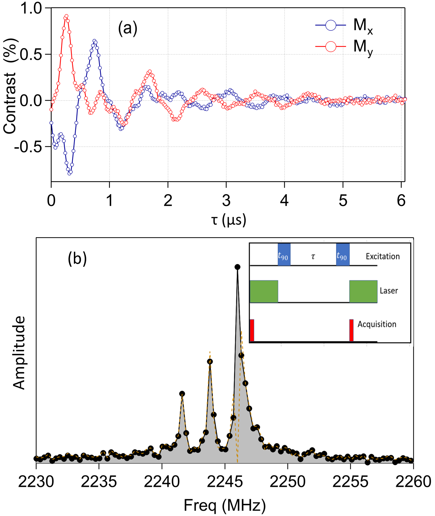
Figure 6: (a) Change in fluorescence contrast as a function of pulse spacing, $\tau$, for a Ramsey sequence at the $|0\rangle\leftrightarrow|-1\rangle$ transition of an NV in a field of 22 mT at ambient pressure. $M_{x}$ and $M_{y}$ are measured using different phases (90^∘) for the second microwave pulse. Panel (b) shows the amplitude of the complex Fourier transform of the data in (a), revealing three separate peaks corresponding to the three $I_{z}$ states of the ¹⁴N nuclei coupled to the NV electronic spin. The dashed brown line shows the spectrum measured without phase cycling.

By controlling the phase of the second pulse relative to the first, one can project either $\langle S_{x}\rangle$ or $\langle S_{y}\rangle$ onto the $z$ axis. Collecting data for both phases enables quadrature detection and hence the full complex Fourier transform can be obtained. It is also useful to implement phase cycling to improve the signal-to-noise ratio. Spurious noise, misalignments of the microwave pulses, and astigmatism in the phase response of the microwave sources can all contribute to noise in the measured fluorescence contrast, and similar approaches are regularly used in conventional magnetic resonance [32]. By cycling the phases of the first and second $\mathbf{H}_{1}$ pulses so that the NV spin is rotated alternately to the $\pm x$ and $\pm y$ directions and back to the $\pm z$ direction, one can either add or subtract the measured contrast to remove background noise. Fig. 6 demonstrates this approach. Note that the spectrum of the NV reveals three separate peaks, which arise due to the hyperfine coupling between the NV spin, $S$, and the ¹⁴N nuclear spin, $I=1$ (natural abundance 99.6%). The hyperfine coupling is given by $\mathcal{H}_{hf}=\hat{\mathbf{S}}\cdot\mathbb{A}\cdot\hat{\mathbf{I}}$, where the coupling tensor $\mathbb{A}$ is diagonal along the NV-axis with components $A_{||}=2.1$ and $A_{\perp}=2.3$ MHz [33]. The three peaks correspond to NV spins in the ensemble for which $I_{z}=$ -1, 0 or +1 and hence a hyperfine field of 0, $\pm 2.1$MHz shifts the resonant frequency.

Figure 7: Spectra of the $|0\rangle\leftrightarrow|-1\rangle$ transition of the NV ensemble as a function of pressure, measured by echo sequences. The spectrum at 5.96 GPa was measured by continuous wave, since the antenna leads were thinned out under the pressure from the anvils, reducing the the Rabi frequency.

Spectra of the $|0\rangle\leftrightarrow|-1\rangle$ transition under pressure are shown in Fig. 7. The resonance frequency of this transition is given by $f_{0}=D-\gamma_{e}H_{0}$, where $D$ is the zero-field splitting, $\gamma_{e}$ is the electron gyromagnetic ratio, and $H_{0}=29$ mT is the magnitude of the applied field. $D$ increases linearly with pressure [23, 24], which enables us to use the shift of the resonance as a measure of the pressure. In this case we use the ambient pressure value of $D(0)=2866$ MHz and $dD/dP=11.72$ MHz/GPa. The spectra clearly broaden with pressure, and the three peaks are no longer resolvable under pressure. We find that the linewidths increase by a factor of eight over this range, corresponding to a pressure variation of approximately 15% over the volume of the sample. The non-hydrostaticity is likely due to freezing of the pressure medium (Daphne oil 7575), which freezes above 3 GPa at room temperature. Above 5.5 GPa, we found that the Rabi frequency dropped significantly as the leads to the antenna become clipped under pressure. Utilizing thinner leads in the future may alleviate this problem.

III.2 Dynamical decoupling

In the rotating frame, the NV spins will precess around $\mathbf{B}_{ac}(t)$ (Eq. (1)) and acquire a phase $\Phi(t)=\gamma\int_{0}^{t}B_{ac}(t^{\prime})dt^{\prime}$. A 180^∘ pulse will effectively reverse the direction of $\mathbf{B}_{ac}(t)$, and reverse the direction of precession. For a series of 180^∘ pulses spaced at regular intervals, $\tau$, the phase of the NV can be written as [29]:

$$\Phi(t)=\gamma\int_{0}^{t}B_{eff}(t^{\prime})dt^{\prime},$$ (2)

where the effective field is $B_{eff}(t)=u(t)B_{ac}(t)$, and $u(t)$ alternates between $\pm 1$ between successive 180^∘ pulses (which we approximate as infinitely-narrow in time). The effective field can be expressed as:

$$B_{eff}(t) = B_{ac}\sum_{n=1,3,\cdots}\frac{2}{n\pi}\left[\cos((\omega_{ac}-{n\pi/\tau})t-\phi_{ac})\right.$$ (3)

$$\left.-\cos((\omega_{ac}+{n\pi/\tau})t+\phi_{ac})\right].$$

Most of these frequency components will integrate to zero in Eq. 2, which reflects that fact that such pulse sequences filter out noise sources with frequency components far from ${n\pi/\tau}$. On the other hand, if ${n\pi/\tau}\approx\omega_{ac}$, then $B_{eff}(t)$ has a component that is nearly constant over time and the phase $\Phi$ will not integrate to zero. For $n=1$, where the pulse spacing $\tau\approx\pi/\omega_{ac}$,

$$\Phi(t)=\frac{2\gamma B_{ac}t}{\pi}{\mathrm{sinc}}(\pi\delta ft)\cos(\pi\delta ft-\phi_{ac})$$ (4)

where $\delta f=(2\tau)^{-1}-\omega_{ac}/(2\pi)$ is the frequency offset. If the pulse spacing is tuned exactly such that $\delta f=0$, then the phase will accumulate linearly with time. After accumulating this phase for a series of $N$ pulses, the NV magnetization can be then be projected to the $z$ axis. At the end of the sequence, the NV magnetization depends on the relative phase of the first and last $90^{\circ}$ pulses, and that the fluorescence contrast varies as:

$$\Delta I\sim\begin{cases}\cos\left(2N\frac{\gamma B_{ac}}{\omega_{ac}}\cos\phi_{ac}\right)&\text{for }90_{x}-90_{x}\\ \sin\left(2N\frac{\gamma B_{ac}}{\omega_{ac}}\cos\phi_{ac}\right)&\text{for }90_{x}-90_{y}\\ \end{cases}$$ (5)

For typical values of $\omega_{ac}=2\pi\cdot 100$ kHz with amplitude $B_{ac}=$15 nT and $N=48$ refocusing pulses, the fluorescence contrast will be reduced by 0.1% for the $90_{x}-90_{y}$ sequence, assuming no coherence decay.

III.3 Pulse spacing sweep

Figure 8: (Upper panel) Optical contrast, $\Delta I$ measured in a DAC measured versus detection frequency, $(2\tau)^{-1}$, where $\tau$ is the pulse spacing of a dynamical decoupling sequence. Input signals of 1.12 and 1.25 MHz were introduced externally. The dip in the contrast arises due to the phase accumulated by the NV centers. (Lower panel) Optical contrast, $\Delta I$ of a test AC signal measured by signal averaging as a function of the voltage applied to the AC coil. The solid purple line is a fit to a Bessel function as described in the text.

The most straightforward approach to detecting an AC field is to sweep the pulse spacing, $\tau$, and search for changes in $\Delta I$, as illustrated in Fig. 8. In this case, multiple measurements of the signal contrast are averaged, while a CW external field is applied via a small loop located near the sample space in the diamond anvil cell. The phase, $\phi_{ac}$ is randomly distributed, depending on the time at which the NV detection sequence is initiated. In this case, for the $90_{x}-90_{x}$ sequence, the fluorescence contrast is given by:

$$\Delta I=1-J_{0}(N{\gamma B_{ac}}/{\omega_{ac}}),$$ (6)

where $J_{0}(x)$ is a Bessel function of the first kind. For the $90_{x}-90_{y}$ sequence $\Delta I=0$. This behavior is illustrated in the lower panel of Fig. 8, in which the AC voltage, $V_{pp}$ is varied to change the magnitude of $B_{ac}$. In this case, $B_{ac}\propto V_{pp}$, however the coefficient is unknown.

Figure 9 shows AC spectra in the absence of an external driving AC field at ambient pressure, 3.6 GPa and 5.0 GPa respectively. There is a dip in the contrast at $\sim 0.3$ MHz, which corresponds to the Larmor frequency of ¹³C in the applied $H_{0}$ field. The 1% abundant ¹³C nuclear spins in the diamond lattice precess at this frequency and create AC fields at the NV site that are not refocused by the dynamical decoupling. The dip around 1.2 MHz is likely due to hydrogen in the pressure medium.

Figure 9: Optical contrast versus frequency, $(2\tau)^{-1}$, where $\tau$ is the pulse spacing of an XY8-16 sequence, measured at various pressures. The dip s around 0.3 MHz and 1.2 MHz arises from precessing ¹³C spins in the diamond lattice and ¹H spins in the pressure medium, respectively.

III.4 Synchronized Readout

Figure 10: (a) Optical contrast, $\Delta I$ measured for NVs in the DAC with a test signal at frequency $f_{ac}=1.2001$ MHz, where $\tau=416.667$ ns (corresponding to a detection frequency at 1.2 MHz), for a sequence of equally-spaced measurements at with $T_{meas}=45$ $\mu$s, as described in the text. (b) Fourier transform of $\Delta I$ at ambient pressure. The spectra exhibits a single large peak at 100 Hz, and the vertical axis has been scaled to match the known applied field magnitude. The 3.61 GPa data has been offset vertically by 500 nT for clarity. (c) Sensitivity, $\eta$ ($\bullet$), versus pressure. The dashed blue line corresponds to the necessary sensitivity to achieve unity signal to noise ratio after 1 minute, and the pink square ($\blacksquare$) at 0 GPa corresponds to the sensitivity reported in [30].

Instead of averaging the signal over randomly-distributed initial phases at the beginning of each repeat of the dynamical decoupling sequence, it is possible to collect each fluorescence measurement and perform a Fourier transform. After each NV fluorescence measurement, the NV is re-initialized into the ground state without affecting the AC source. As a result, the phase of $\mathbf{B}_{ac}(t)$ will evolve in a coherent fashion for each measurement. The slowest varying component of the effective field in Eq. 3 will acquire a phase $\phi_{m}=2\pi\delta fmT_{meas}-\phi_{ac}$, where $T_{meas}$ is the measurement repeat time, and $m$ is the $m^{th}$ measurement. In this case, $\Phi_{m}\approx\frac{2\gamma B_{ac}T_{meas}}{\pi}\cos\phi_{m}$. For a $90_{x}-90_{y}$ sequence in the limit of small $B_{ac}$, the fluorescence contrast will vary as:

$$\Delta I(T)\sim\left(\frac{2N\gamma B_{ac}}{\omega_{ac}}\right)\cos(2\pi\delta fT-\phi_{ac}),$$ (7)

where $T=mT_{meas}$. This behavior is illustrated in Fig. 10 both at ambient pressure and at 3.6 GPa. In effect, the AC field is demodulated by the dynamical decoupling sequence, and imprinted on $\Delta I$. A Fourier transform of $\Delta I(T)$ thus provides a spectrum of $B_{ac}(t)$ relative to the detection frequency $(2\tau)^{-1}$. This detection scheme is often referred to as ‘quantum heterodyne’ [31, 34]. The frequency resolution is determined by the number of points $m$, $T_{meas}$, the stability of the field $\mathbf{H}_{0}$, and the stability of the microwave pulse timing. The resolution can be as low as a mHz, which is sufficient to resolve many chemical shifts even at low applied fields [31, 30]. This technique requires coherently averaging many repeated measurements, but sufficient signal-to-noise ratio can be obtained within a few hours.

In practice, the minimum detectable frequency , $\omega_{ac}$, is bounded by $T_{2}$ because the NV magnetization will decay over during the free precession time, $\tau$, giving rise to another factor of $e^{-\pi/\omega_{ac}T_{2}}$. For our NV diamond we have $T_{2}\approx 200\mu$s, corresponding to a minimum frequency $\sim 10$ kHz. The maximum detectable frequency is bounded by the shortest possible pulse spacing, which is approximately equal to the 180^∘ pulse time, determined by the Rabi frequency. In our case the maximum detectable frequency $\sim 10$ MHz. Note that there is an upper limit to the heterodyne frequency, $\delta f$, based upon the minimum time between consecutive measurements. This limit is set by the time to measure the fluorescence, which is usually a few $\mu$s.

III.5 Sensitivity Measurements

The data shown in Fig. 10 was acquired for a large applied test AC field for a single acquisition sequence without signal averaging with a total measurement time of approximately 1.5 s, corresponding to a sensitivity, $\eta=1.9$ nT/$\sqrt{\mathrm{Hz}}$ at ambient pressure. At 3.6 GPa, we find the sensitivity decreases to $\eta=7.6$ nT/$\sqrt{\mathrm{Hz}}$. Here we define sensitivity as the minimum detectable signal per unit time. Ideally $\eta$ should be as low as possible to achieve a high signal to noise ratio. Our values are not as low as previous reports, which reach down to 32 pT/$\sqrt{\mathrm{Hz}}$ [30]. One of the primary reasons for the difference in the DAC is the wide distribution of Rabi frequencies, which means that not all of the NVs in the ensemble experience the same $H_{1}$ field. The pulse width for the dynamical decoupling 180^∘ pulses, given by $\pi/(\gamma H_{1})$, will differ for each of these NVs. As a result, the accumulated phase in Eq. 2 is not as high as it would be for a uniform $H_{1}$. To illustrate this point, Fig. 11 shows how the signal intensity varies as a function of the pulse width time. Numerical simulations of the Bloch equations under these conditions indicate that the sensitivity is reduced by $\approx 10$% if the dynamical decoupling pulses are either 10% shorter or longer than ideal. As shown in Fig. 5, the $H_{1}$ field for the straight antenna is inhomogeneous over the sample volume, such that the width of the distribution is approximately 40% of the average. Although this antenna is able to provide large $H_{1}$ fields within the sample space, the field inhomogeneity reduces the synchronized readout sensitivity.

Figure 11: Signal intensity (arbitrary units) for a synchronized readout measurement of an AC signal (as in Fig. 10) versus the width of a 90^∘ pulse. The dynamical decoupling pulses ($180^{\circ}$) are twice as long as the time $t_{90}$ given on the horizontal axis.

Another limiting factor for the sensitivity is the large ratio of the 180^∘ pulse width, $t_{180}$, to the pulse spacing, $\tau$. The data in Fig. 10 utilized $t_{180}/\tau\approx 0.43$, which is far from the idealized case of the infinitely-narrow pulses that would give rise to the effective field in Eq. 3. Numerical simulations indicate that the sensitivity will be suppressed when the ratio $t_{180}/\tau\gtrsim 0.2$. This provides an effective upper limit on $\omega_{ac}^{max}\approx 0.2\Omega$ for a given value of the Rabi frequency, $\Omega$.

The lower limit for the sensitivity is determined by $T_{2}$ because the NV magnetization will decay during the free precession time between the dynamical decoupling pulses. This leads to a exponential prefactor of $e^{-\pi/\omega_{ac}T_{2}}$ for Eq. 7, and an effective lower limit $\omega_{ac}^{min}\approx\pi/\ln(10)T_{2}$, where the sensitivity is reduced by a factor of 10. For our NV sample with $T_{2}\approx 200$ $\mu$s and $\Omega\approx 3$ MHz, we have $f_{ac}^{min}\approx 1$ kHz and $f_{ac}^{max}\approx 0.5$ MHz. For detection of precessing nuclear spins such as ${}^{1}H$ or ¹⁹F, $H_{0}$ should lie between 0.02 and 25 mT in order to achieve $\omega_{ac}$ in this range. Curiously, except for small frequencies where $T_{2}$ limits the sensitivity, the fluorescence contrast maximum in Eq. 7 does not depend on the applied field, $H_{0}$, because both $B_{ac}$ and $\omega_{ac}$ are proportional to $H_{0}$ (for thermally polarized nuclei).

Under pressure we find that $\eta$ increases by a factor of four, as shown in Fig. 10(c). There are two possible reasons for this change. Under pressure the NV spectrum is broadened due to the pressure gradients. If the spectrum is sufficiently broad, the dynamical decoupling pulses will not fully refocus the NV magnetization, similar to the effect of a non-uniform $H_{1}$ field as discussed above. Moreover, the antenna deforms under pressure, and as a result the impedance changes and affects the magnitude of the $H_{1}$ field. Consequently both $\Omega$ and $\Delta I$ can be reduced, affecting the sensitivity.

IV Discussion and Conclusions

We have demonstrated AC-ODMR in a DAC with a sensitivity of 1.9 nT$/\sqrt{\mathrm{Hz}}$, which is about 50 times larger than values reported for other NV-based AC sensors operating under ambient conditions. To detect nuclear spins external to the diamond, it is possible to either initialize these with a 90^∘ pulse at the nuclear Larmor frequency ($\sim 1$ MHz) in order to let them precess coherently, or to use correlation spectroscopy to detect their noise fluctuations. The magnitude of $B_{ac}$ can be estimated assuming that the NV diamond chip is embedded in a spherical volume of uniform nuclear magnetization, $\mathbf{M}(t)$, that is precessing at Larmor frequency $\omega_{ac}$. In this case, $B_{ac}=\frac{8\pi}{3}\chi_{N}H_{0}$, where $\chi_{N}={\rho\gamma_{n}^{2}\hbar^{2}I(I+1)}/{3k_{B}T}$ is the Curie susceptibility of nuclei with spin $I$, and number density $\rho$. For hydrogen in water at room temperature in a field of 10 mT, $B_{ac}\approx 27$ pT. To achieve a signal to noise ratio of unity with our demonstrated sensitivity $\eta=1.9$ nT$/\sqrt{\mathrm{Hz}}$ would require signal averaging for a time $T_{avg}=(\eta/B_{ac})^{2}\sim 80$ min. The dashed blue line in Fig. 10(c) shows the maximum $\eta$ necessary to achieve a minimum signal to noise ratio of unity within one minute. It is clear that an order of magnitude reduction in $\eta$ will be necessary to avoid hours of signal averaging. Note that although conventional NMR has sensitivities on the order of 10 pT/$\sqrt{\mathrm{Hz}}$ [29], this quantity scales as $\eta_{NMR}\sim V_{s}^{-1/2}$, where $V_{s}$ is the sample volume [35]. For a 100 $\mu$m coil diameter and sample volume of 1 nL at a field of 10 mT, we estimate $\eta_{NMR}\approx 85$ nT/$\sqrt{\mathrm{Hz}}$ [36], approximately two orders of magnitude higher than our measurement.

There are several possible routes to improve the sensitivity of AC-ODMR in the DAC. The inhomogeneity of the microwave fields from the antenna leads to an increase in $\eta$. An antenna design that provides a more homogeneous and stable $H_{1}$ field and is less prone to distortions under pressure is vital. In the future other antenna designs may be considered, for example a circular loop within the sample space, to improve the homogeneity and reduce screening effects by the gasket. Utilizing diamonds with lower NV concentrations and isotopically pure ¹²C would significantly enhance $T_{2}$ and also improve the sensitivity. It is also possible to improve the sensitivity by utilizing dynamic nuclear polarization. This number can be enhanced significantly by utilizing the presence of free radicals and taking advantage of the Overhauser effect to transfer polarization to the nuclear spins in a liquid. Bucher et al. used the TEMPOL molecule dissolved into liquid solutions to enhance the sensitivity by more than a factor of 200 [37]. The unpaired electrons on the TEMPOL molecule have an enhanced spin polarization that can be transferred to hyperpolarize the nuclear spins beyond their thermal polarization described by $\chi_{N}$. This process can enhance the signal-to-noise ratio by several orders of magnitude, but requires pulsing the system at the Larmor frequency of the TEMPOL electron spins for several ms prior to detection of the nuclear spins with NV magnetometry.

The sensitivity may also be improved by utilizing double quantum coherence under pressure [38, 39]. The AC-ODMR experiments described here are based on single quantum coherence in which the NV is prepared in the state $|0\rangle+|\pm 1\rangle$. The resonance frequency of the double quantum coherent state $|-1\rangle+|+1\rangle$ is independent of $D$. This property could be important because pressure inhomogeneities strongly affect $D$, giving rise to spectral broadening that impacts the sensitivity of the AC detection. Utilizing dynamical decoupling at the double quantum coherent frequency would allow the NV ensemble to precess and acquire phase more homogeneously and may enable a reduction in $\eta$ even in the presence of strong pressure gradients. It may also be prudent to utilize shaped pulses with the arbitrary waveform generator, which have a broader frequency response and may be able to better refocus the NV magnetization in the presence of inhomogeneous broadening [40].

In addition to the zero-field splitting, $D$, the zero-phonon emission line (637 nm at ambient pressure and temperature) is also pressure dependent [15, 24]. Both quantities can be used to measure the pressure, eliminating the need for other manometers such as Ruby chips within the sample space or the high-frequency edge of the Raman spectra of the diamond anvil [41, 42]. For ODMR, the microwave frequency needs to be adjusted after each pressure change (by 100 GPa it will have increased by 1.2 GHz). This shift may necessitate adjusting different microwave components, such as the amplifier and filters. The emission wavelength shifts down with pressure and reaches 532 nm at approximately 60 GPa [23]. To operate at higher pressures it is thus necessary to switch to a lower wavelength excitation laser. It is common to utilize an optical filter before the detector, which needs to be adjusted with increasing pressures.

AC-ODMR under pressure will enable a broad range of NMR experiments at pressures that have not been possible previously. In particular it should be possible to to test geochemical predictions about fluid chemistry modifying the Earth’s crust. These predictions extend now to 6.0 GPa and 1200 C [43, 44, 45], and are testable only via vibrational and optical spectroscopic measurements, and not NMR [46, 47]. High-pressure NMR spectroscopy via conventional detection is a familiar tool in inorganic solution chemistry [48, 49, 50], but the pressures are less than $\sim 0.4$ GPa, except for a few studies [51, 52, 53, 54]. As discussed above, diamond-anvil cell (DAC) technology can reach higher pressures, but the sample volumes are too small for NMR detection via Faraday coils, which is why optical detection via AC-ODMR is potentially so valuable, particularly if it is coupled to methods of polarization transfer that enhance the signals. An additional benefit is that experiments are now possible on solutions that would be dangerous in larger amounts.

V Acknowledgements

We thank A. Ajoy, S. Gomez-Diaz, P. Klavins, V. Norman and M. Radulaski for stimulating discussions. The work was supported by the United States Department of Energy, Office of Basic Energy Sciences, Chemical Sciences, Geosciences and Biosciences Division for Grant DE-FG0205ER15693. The data that support the findings of this study are available from the corresponding author upon reasonable request.

References

- Meier et al. [2011] B. Meier, S. Greiser, J. Haase, T. Herrmannsdörfer, F. Wolff-Fabris, and J. Wosnitza, NMR signal averaging in 62T pulsed fields, J. Magn. Reson. 210, 1 (2011).
- Meier [2018] T. Meier, At its extremes: NMR at giga-pascal pressures, in Annual Reports on NMR Spectroscopy (Elsevier, 2018) pp. 1–74.
- Lin et al. [2015] C. H. Lin, K. R. Shirer, J. Crocker, A. P. Dioguardi, M. M. Lawson, B. T. Bush, P. Klavins, and N. J. Curro, Evolution of hyperfine parameters across a quantum critical point in , Phys. Rev. B 92, 155147 (2015).
- Ochoa et al. [2015] G. Ochoa, C. D. Pilgrim, M. N. Martin, C. A. Colla, P. Klavins, M. P. Augustine, and W. H. Casey, 2H and 139La NMR spectroscopy in aqueous solutions at geochemical pressures, Angew. Chem. Int. Ed. 54, 15444 (2015).
- Fujiwara et al. [1980] H. Fujiwara, H. Kadomatsu, and K. Tohma, Simple clamp pressure cell up to 30 kbar, Rev. Sci. Instrum. 51, 1345 (1980).
- Kobayashi et al. [2007] T. C. Kobayashi, H. Hidaka, H. Kotegawa, K. Fujiwara, and M. I. Eremets, Nonmagnetic indenter-type high-pressure cell for magnetic measurements, Rev. Sci. Instrum. 78, 23909 (2007).
- Eremets [1996] M. Eremets, High pressure experimental methods (Oxford University Press, 1996).
- Meier et al. [2015] T. Meier, S. Reichardt, and J. Haase, High-sensitivity NMR beyond 200,000 atmospheres of pressure, J. Magn. Reson. 257, 39 (2015).
- Hoult and Richards [1976a] D. I. Hoult and R. Richards, The signal-to-noise ratio of the nuclear magnetic resonance experiment, Journal of Magnetic Resonance (1969) 24, 71 (1976a).
- Meier et al. [2018] T. Meier, S. Khandarkhaeva, S. Petitgirard, T. Körber, A. Lauerer, E. Rössler, and L. Dubrovinsky, NMR at pressures up to 90 GPa, J. Magn. Reson. 292, 44 (2018).
- Meier et al. [2019] T. Meier, S. Khandarkhaeva, J. Jacobs, N. Dubrovinskaia, and L. Dubrovinsky, Improving resolution of solid state NMR in dense molecular hydrogen, Appl. Phys. Lett. 115, 131903 (2019).
- Drozdov et al. [2015] A. P. Drozdov, M. I. Eremets, I. A. Troyan, V. Ksenofontov, and S. I. Shylin, Conventional superconductivity at 203 kelvin at high pressures in the sulfur hydride system, Nature 525, 73 (2015).
- Drozdov et al. [2019] A. P. Drozdov, P. P. Kong, V. S. Minkov, S. P. Besedin, M. A. Kuzovnikov, S. Mozaffari, L. Balicas, F. F. Balakirev, D. E. Graf, V. B. Prakapenka, E. Greenberg, D. A. Knyazev, M. Tkacz, and M. I. Eremets, Superconductivity at 250 K in lanthanum hydride under high pressures, Nature 569, 528 (2019).
- Somayazulu et al. [2019] M. Somayazulu, M. Ahart, A. K. Mishra, Z. M. Geballe, M. Baldini, Y. Meng, V. V. Struzhkin, and R. J. Hemley, Evidence for superconductivity above 260 K in lanthanum superhydride at megabar pressures, Phys. Rev. Lett. 122, 027001 (2019).
- Doherty et al. [2013] M. W. Doherty, N. B. Manson, P. Delaney, F. Jelezko, J. Wrachtrup, and L. C. Hollenberg, The nitrogen-vacancy colour centre in diamond, Phys. Rep. 528, 1 (2013).
- Matsuzaki et al. [2016] Y. Matsuzaki, H. Morishita, T. Shimooka, T. Tashima, K. Kakuyanagi, K. Semba, W. J. Munro, H. Yamaguchi, N. Mizuochi, and S. Saito, Optically detected magnetic resonance of high-density ensemble of NV-centers in diamond, J. Phys.: Condens. Matter 28, 275302 (2016).
- Bucher et al. [2019] D. B. Bucher, D. P. L. A. Craik, M. P. Backlund, M. J. Turner, O. B. Dor, D. R. Glenn, and R. L. Walsworth, Quantum diamond spectrometer for nanoscale NMR and ESR spectroscopy, Nat Protoc 14, 2707 (2019).
- Childress and Hanson [2013] L. Childress and R. Hanson, Diamond NV centers for quantum computing and quantum networks, MRS Bulletin 38, 134 (2013).
- Lesik et al. [2019] M. Lesik, T. Plisson, L. Toraille, J. Renaud, F. Occelli, M. Schmidt, O. Salord, A. Delobbe, T. Debuisschert, L. Rondin, P. Loubeyre, and J.-F. Roch, Magnetic measurements on micrometer-sized samples under high pressure using designed NV centers, Science 366, 1359 (2019).
- Hsieh et al. [2019] S. Hsieh, P. Bhattacharyya, C. Zu, T. Mittiga, T. J. Smart, F. Machado, B. Kobrin, T. O. Höhn, N. Z. Rui, M. Kamrani, S. Chatterjee, S. Choi, M. Zaletel, V. V. Struzhkin, J. E. Moore, V. I. Levitas, R. Jeanloz, and N. Y. Yao, Imaging stress and magnetism at high pressures using a nanoscale quantum sensor, Science 366, 1349 (2019).
- Shang et al. [2019] Y.-X. Shang, F. Hong, J.-H. Dai, Hui-Yu, Y.-N. Lu, E.-K. Liu, X.-H. Yu, G.-Q. Liu, and X.-Y. Pan, Magnetic sensing inside a diamond anvil cell via nitrogen-vacancy center spins, Chinese Phys. Lett. 36, 086201 (2019).
- Yip et al. [2019] K. Y. Yip, K. O. Ho, K. Y. Yu, Y. Chen, W. Zhang, S. Kasahara, Y. Mizukami, T. Shibauchi, Y. Matsuda, S. K. Goh, and S. Yang, Measuring magnetic field texture in correlated electron systems under extreme conditions, Science 366, 1355 (2019).
- Doherty et al. [2014] M. W. Doherty, V. V. Struzhkin, D. A. Simpson, L. P. McGuinness, Y. Meng, A. Stacey, T. J. Karle, R. J. Hemley, N. B. Manson, L. C. L. Hollenberg, and S. Prawer, Electronic properties and metrology applications of the diamond center under pressure, Phys. Rev. Lett. 112, 047601 (2014).
- Steele et al. [2017] L. G. Steele, M. Lawson, M. Onyszczak, B. T. Bush, Z. Mei, A. P. Dioguardi, J. King, A. Parker, A. Pines, S. T. Weir, W. Evans, K. Visbeck, Y. K. Vohra, and N. J. Curro, Optically detected magnetic resonance of nitrogen vacancies in a diamond anvil cell using designer diamond anvils, Appl. Phys. Lett. 111, 221903 (2017).
- Weir et al. [2000] S. T. Weir, J. Akella, C. Aracne-Ruddle, Y. K. Vohra, and S. A. Catledge, Epitaxial diamond encapsulation of metal microprobes for high pressure experiments, Appl. Phys. Lett. 77, 3400 (2000).
- Ibarra et al. [1997] A. Ibarra, M. Gonzalez, R. Vila, and J. Molla, Wide frequency dielectric properties of cvd diamond, Diam. Relat. Mater. 6, 856 (1997).
- Meier and Haase [2015] T. Meier and J. Haase, Anvil cell gasket design for high pressure nuclear magnetic resonance experiments beyond 30 GPa, Rev. Sci. Instrum. 86, 123906 (2015).
- Meier et al. [2017] T. Meier, N. Wang, D. Mager, J. G. Korvink, S. Petitgirard, and L. Dubrovinsky, Magnetic flux tailoring through Lenz lenses for ultrasmall samples: A new pathway to high-pressure nuclear magnetic resonance, Sci. Adv. 3, eaao5242 (2017).
- Degen et al. [2017] C. L. Degen, F. Reinhard, and P. Cappellaro, Quantum sensing, Rev. Modern Phys. 89, 035002 (2017).
- Glenn et al. [2018] D. R. Glenn, D. B. Bucher, J. Lee, M. D. Lukin, H. Park, and R. L. Walsworth, High-resolution magnetic resonance spectroscopy using a solid-state spin sensor, Nature 555, 351 (2018).
- Schmitt et al. [2017] S. Schmitt, T. Gefen, F. M. Stürner, T. Unden, G. Wolff, C. Müller, J. Scheuer, B. Naydenov, M. Markham, S. Pezzagna, J. Meijer, I. Schwarz, M. Plenio, A. Retzker, L. P. McGuinness, and F. Jelezko, Submillihertz magnetic spectroscopy performed with a nanoscale quantum sensor, Science 356, 832 (2017).
- Bain [1984] A. D. Bain, Coherence levels and coherence pathways in NMR. a simple way to design phase cycling procedures, Journal of Magnetic Resonance (1969) 56, 418 (1984).
- Felton et al. [2009] S. Felton, A. M. Edmonds, M. E. Newton, P. M. Martineau, D. Fisher, D. J. Twitchen, and J. M. Baker, Hyperfine interaction in the ground state of the negatively charged nitrogen vacancy center in diamond, Phys. Rev. B 79, 075203 (2009).
- Norman et al. [2020] V. A. Norman, S. Majety, Z. Wang, W. H. Casey, N. Curro, and M. Radulaski, Novel color center platforms enabling fundamental scientific discovery, InfoMat , 1– 24 (2020).
- Hoult and Richards [1976b] D. Hoult and R. Richards, The signal-to-noise ratio of the nuclear magnetic resonance experiment, Journal of Magnetic Resonance (1969) 24, 71 (1976b).
- Peck et al. [1995] T. L. Peck, R. L. Magin, and P. C. Lauterbur, Design and analysis of microcoils for nmr microscopy, Journal of Magnetic Resonance, Series B 108, 114 (1995).
- Bucher et al. [2020] D. B. Bucher, D. R. Glenn, H. Park, M. D. Lukin, and R. L. Walsworth, Hyperpolarization-enhanced NMR spectroscopy with femtomole sensitivity using quantum defects in diamond, Phys. Rev. X 10, 021053 (2020).
- Mamin et al. [2014] H. Mamin, M. Sherwood, M. Kim, C. Rettner, K. Ohno, D. Awschalom, and D. Rugar, Multipulse double-quantum magnetometry with near-surface nitrogen-vacancy centers, Phys. Rev. Lett. 113, 030803 (2014).
- Marshall et al. [2021] M. C. Marshall, R. Ebadi, C. Hart, M. J. Turner, M. J. H. Ku, D. F. Phillips, and R. L. Walsworth, High-precision mapping of diamond crystal strain using quantum interferometry (2021), arXiv:2108.00304 [quant-ph] .
- Spindler et al. [2017] P. E. Spindler, P. Schöps, W. Kallies, S. J. Glaser, and T. F. Prisner, Perspectives of shaped pulses for EPR spectroscopy, J. Magn. Reson. 280, 30 (2017).
- Syassen [2008] K. Syassen, Ruby under pressure, High Pressure Res. 28, 75 (2008).
- Akahama and Kawamura [2006] Y. Akahama and H. Kawamura, Pressure calibration of diamond anvil Raman gauge to 310GPa, J. Appl. Phys. 100, 043516 (2006).
- Sverjensky et al. [2014] D. A. Sverjensky, B. Harrison, and D. Azzolini, Water in the deep earth: the dielectric constant and the solubilities of quartz and corundum to 60 kb and 1200 C, Geochim. Cosmochim. Acta 129, 125 (2014).
- Sverjensky and Huang [2015] D. A. Sverjensky and F. Huang, Diamond formation due to a pH drop during fluid–rock interactions, Nat Commun 6, 1 (2015).
- Pan et al. [2013] D. Pan, L. Spanu, B. Harrison, D. A. Sverjensky, and G. Galli, Dielectric properties of water under extreme conditions and transport of carbonates in the deep earth, Proc. Natl. Acad. Sci. 110, 6646 (2013).
- Facq et al. [2014] S. Facq, I. Daniel, G. Montagnac, H. Cardon, and D. A. Sverjensky, In situ Raman study and thermodynamic model of aqueous carbonate speciation in equilibrium with aragonite under subduction zone conditions, Geochim. Cosmochim. Acta 132, 375 (2014).
- Facq et al. [2016] S. Facq, I. Daniel, G. Montagnac, H. Cardon, and D. A. Sverjensky, Carbon speciation in saline solutions in equilibrium with aragonite at high pressure, Chem. Geol. 431, 44 (2016).
- Asano and Le Noble [1978] T. Asano and W. Le Noble, Activation and reaction volumes in solution, Chem. Rev. 78, 407 (1978).
- Van Eldik et al. [1989] R. Van Eldik, T. Asano, and W. Le Noble, Activation and reaction volumes in solution. 2, Chem. Rev. 89, 549 (1989).
- Drljaca et al. [1998] A. Drljaca, C. Hubbard, R. Van Eldik, T. Asano, M. Basilevsky, and W. Le Noble, Activation and reaction volumes in solution. 3, Chem. Rev. 98, 2167 (1998).
- Jonas [1980] J. Jonas, Nuclear magnetic resonance studies at high pressures (modern aspects of physical chemistry at high pressure: the 50th commemorative volume), The Review of Physical Chemistry of Japan 50, 19 (1980).
- Lang and Lüdemann [1977] E. Lang and H.-D. Lüdemann, Pressure and temperature dependence of the longitudinal proton relaxation times in supercooled water to -87∘ C and 2500 bar, J. Chem. Phys. 67, 718 (1977).
- De Langen and Prins [1995] M. De Langen and K. Prins, NMR probe for high pressure and high temperature, Rev. Sci. Instrum. 66, 5218 (1995).
- Ballard et al. [1998] L. Ballard, A. Yu, C. Reiner, and J. Jonas, A high-pressure, high-resolution NMR probe for experiments at 500 MHz, J. Magn. Reson. 133, 190 (1998).