On Association between Absolute and Relative Zigzag Persistence

Abstract

Duality results [5, 6] connecting persistence modules for absolute and relative homology provides a fundamental understanding into persistence theory. In this paper, we study similar associations in the context of zigzag persistence. Our main finding is a weak duality for the so-called non-repetitive zigzag filtrations in which a simplex is never added again after being deleted. The technique used to prove the duality for non-zigzag persistence does not extend straightforwardly to our case. Accordingly, taking a different route, we prove the weak duality by converting a non-repetitive filtration to an up-down filtration by a sequence of diamond switches [2]. We then show an application of the weak duality result which gives a near-linear algorithm for computing the $p$-th and a subset of the $(p-1)$-th persistence for a non-repetitive zigzag filtration of a simplicial $p$-manifold. Utilizing the fact that a non-repetitive filtration admits an up-down filtration as its canonical form, we further reduce the problem of computing zigzag persistence for non-repetitive filtrations to the problem of computing standard persistence for which several efficient implementations exist. Our experiment shows that this achieves substantial performance gain. Our study also identifies repetitive filtrations as instances that fundamentally distinguish zigzag persistence from the standard persistence.

1 Introduction

Standard persistent homology defined over a growing sequence of simplicial complexes is a fundamental tool in topological data analysis (TDA). Since the advent of persistence algorithm [11] and its algebraic understanding [20], various extensions of the basic concept have been explored [2, 3, 5, 6]. These extensions create a need for finding relations among them for a more coherent theory, which can potentially lead to improved algorithms. Two excellent examples catering to this need are the papers by de Silva et al. [6] and Cohen-Steiner et al. [5], which relate standard persistence modules for absolute and relative homology. The original persistence algorithm [11] was designed for absolute homology, but in practice persistence modules involving relative homology do appear [5, 10]. Although the persistence for relative homology can be computed by ‘coning’ on the complexes, the authors of [6] show a duality between the modules arising from absolute and relative homology, thereby revealing an equivalence in their computations.

In this paper, we explore a similar correspondence between the two types of modules but in the context of zigzag persistence. Zigzag persistence introduced by Carlsson and de Silva [2] empowered TDA to deal with filtrations where both insertion and deletion of simplices are allowed. In practice, allowing deletion of simplices does make the topological tool more powerful. For example, in dynamic networks [14], a sequence of graphs may not grow monotonically but can also shrink due to disappearance of vertex connections.

Zigzag persistence possesses some key differences from standard persistence. For example, unlike standard (non-zigzag) modules which decompose into only finite and infinite intervals, zigzag modules decompose into four types of intervals (see Definition 1). This motivates us to have a fresh look at relating zigzag modules arising from absolute and relative homology, and it turns out that the technique used in the non-zigzag case [6] does not extend straightforwardly. Using the Mayer-Vietoris diamond proposed by Carlsson and de Silva [2], we arrive at a duality result which is weak in the sense that an interval from the absolute zigzag module may correspond to two intervals from the relative zigzag module (see Theorem 6). Furthermore, this (weak) duality exists only for the non-repetitive filtrations where a simplex is never inserted again after its deletion (see Definition 4).

We demonstrate an application of the weak duality result by proposing an efficient algorithm for computing zigzag persistence for non-repetitive filtrations of simplicial $p$-manifolds. The algorithm utilizes the Lefschetz duality [5, 19] and a recent near-linear algorithm for zigzag persistence on graphs [9]. It computes all $p$-th intervals and all $(p-1)$-th intervals (except for one type) in near-linear time. This improves the current best time bound of $O(n^{\omega})$ incurred by applying the algorithm for computing general zigzag persistence [16] to this special case.

One insight we gain from proving the weak duality is the fact that a non-repetitive zigzag filtration admits an up-down filtration as its canonical form. We further discover that the up-down filtration can be converted into a non-zigzag filtration and the barcode of the resulting filtration can be related to the original one. This leads to an efficient algorithm for computing zigzag persistence for any non-repetitive filtrations. Note that algorithms for zigzag persistence [3, 15] are more involved (and hence slower in practice) than algorithms for the non-zigzag version though they have the same time complexity [16]. By leveraging our results, we are able to compute zigzag persistence for non-repetitive filtrations using any efficient software for computing standard persistence. In fact, our experiments show that the gain in practice is substantial. However, the reader should be aware of the caveat that the input filtration has to be non-repetitive. The importance of this condition has not been pointed out in the literature before. In a sense, this condition is satisfied by a milder version of zigzag persistence called levelset zigzag [3]. Last but not the least, our finding helps to pinpoint the repetitive filtrations as the instances of zigzag filtrations that fundamentally distinguish zigzag persistence from the standard persistence.

2 Preliminaries

Absolute and relative homology.

We briefly mention some of the algebraic structures adopted in this paper; see [13, 19] for details. All homology groups are taken with coefficient $\mathbb{Z}_{2}$ and therefore vector spaces mentioned in this paper are also over $\mathbb{Z}_{2}$. Let $K$ be a simplicial complex. For $p\geq 0$, $\mathsf{H}_{p}(K)$ denotes the $p$-th homology group of $K$. We also let $\mathsf{H}_{*}(K)$ denote the homology group of all dimensions, i.e., $\mathsf{H}_{*}(K)=\bigoplus_{p\geq 0}\mathsf{H}_{p}(K)$. Relative homology groups are frequently used in this paper. Specifically, given a relative pair of simplicial complexes $(K,L)$ where $L\subseteq K$, we denote the $p$-th relative homology group of $(K,L)$ as $\mathsf{H}_{p}(K,L)$ and denote the relative homology group of all dimensions as $\mathsf{H}_{*}(K,L)$. Sometimes to differentiate, we also call $\mathsf{H}_{p}(K)$ the $p$-th absolute homology group of $K$.

Zigzag module, barcode, and filtration.

A zigzag module [2] (or simply module) is a sequence of vector spaces

$$\mathcal{M}:V_{0}\leftrightarrow V_{1}\leftrightarrow\cdots\leftrightarrow V_{m}$$

in which each $V_{i}\leftrightarrow V_{i+1}$ is a linear map and is either forward, i.e., $V_{i}\to V_{i+1}$, or backward, i.e., $V_{i}\leftarrow V_{i+1}$. It is known [2, 12] that $\mathcal{M}$ has a decomposition of the form $\mathcal{M}\simeq\bigoplus_{k\in\Lambda}\mathcal{I}^{[b_{k},d_{k}]}$, in which each $\mathcal{I}^{[b_{k},d_{k}]}$ is a special type of module called interval module over the interval $[b_{k},d_{k}]$. The (multi-)set of intervals denoted as $\mathsf{Pers}(\mathcal{M}):=\{[b_{k},d_{k}]\,|\,k\in\Lambda\}$ is an invariant of $\mathcal{M}$ and is called the zigzag barcode (or simply barcode) of $\mathcal{M}$. Each interval in a zigzag barcode is called a persistence interval. The following definition characterizes different types of persistence intervals:

Definition 1 (Open and closed birth/death).

Let $\mathcal{M}:V_{0}\leftrightarrow V_{1}\leftrightarrow\cdots\leftrightarrow V_{m}$ be a zigzag module. We call the start of any interval in $\mathsf{Pers}(\mathcal{M})$ as a birth index in $\mathcal{M}$ and call the end of any interval a death index. Moreover, we call a birth index $b$ as closed if $b=0$, or $b>0$ and $V_{b-1}\rightarrow V_{b}$ is a forward map; otherwise, we call $b$ open. Symmetrically, we call a death index $d$ as closed if $d=m$, or $d<m$ and $V_{d}\leftarrow V_{d+1}$ is a backward map; otherwise, we call $d$ open. The types of the birth/death ends classify intervals in $\mathsf{Pers}(\mathcal{M})$ into four types: closed-closed, closed-open, open-closed, and open-open.

Remark 2.

In this paper, we always denote a persistence interval as an interval of integers which is of the form $[b,d]$. Hence, other than the cases when $b=0$ or $d=m$, the designation of open and closed ends of $[b,d]$ is determined by the directions of the maps $V_{b-1}\leftrightarrow V_{b}$, $V_{d}\leftrightarrow V_{d+1}$ in $\mathcal{M}$. Moreover, if $\mathcal{M}$ is the module for the levelset zigzag [3] of a function, then the open and closed ends defined above are the same as the open and closed ends for levelset zigzag.

A zigzag filtration (or simply filtration) is a sequence of simplicial complexes

$$\mathcal{F}:K_{0}\leftrightarrow K_{1}\leftrightarrow\cdots\leftrightarrow K_{m}$$

in which each $K_{i}\leftrightarrow K_{i+1}$ is either a forward inclusion $K_{i}\hookrightarrow K_{i+1}$ or a backward inclusion $K_{i}\hookleftarrow K_{i+1}$. Note that a forward (resp. backward) inclusion in $\mathcal{F}$ can be considered as an addition (resp. deletion) of zero, one, or more simplices. Moreover, we call $\mathcal{F}$ an up-down filtration [3] if $\mathcal{F}$ can be separated into two parts such that the first part contains only forward inclusions and the second part contains only backward ones, i.e., $\mathcal{F}$ is of the form $\mathcal{F}:K_{0}\hookrightarrow K_{1}\hookrightarrow\cdots\hookrightarrow K_{\ell}\hookleftarrow K_{\ell+1}\hookleftarrow\cdots\hookleftarrow K_{m}$.

The $p$-th homology groups induce the $p$-th zigzag module of $\mathcal{F}$

$$\mathsf{H}_{p}(\mathcal{F}):\mathsf{H}_{p}(K_{0})\leftrightarrow\mathsf{H}_{p}(K_{1})\leftrightarrow\cdots\leftrightarrow\mathsf{H}_{p}(K_{m})$$

in which each $\mathsf{H}_{p}(K_{i})\leftrightarrow\mathsf{H}_{p}(K_{i+1})$ is a linear map induced by inclusion. The barcode $\mathsf{Pers}(\mathsf{H}_{p}(\mathcal{F}))$ is also called the $p$-th zigzag barcode of $\mathcal{F}$ and is alternatively denoted as $\mathsf{Pers}_{p}(\mathcal{F}):=\mathsf{Pers}(\mathsf{H}_{p}(\mathcal{F}))$. Each persistence interval in $\mathsf{Pers}_{p}(\mathcal{F})$ is said to have dimension $p$. Frequently in this paper, we consider the homology in all dimensions and take the zigzag module $\mathsf{H}_{*}(\mathcal{F})$, for which we have $\mathsf{Pers}_{*}(\mathcal{F})=\bigsqcup_{p\geq 0}\mathsf{Pers}_{p}(\mathcal{F})$.

Letting $K=\bigcup_{i=0}^{m}K_{i}$, we call $K$ the total complex of $\mathcal{F}$ and call $\mathcal{F}$ a filtration of $K$. Using the total complex, we define the relative filtration $K/\mathcal{F}$ of $\mathcal{F}$ as

$$K/\mathcal{F}:(K,K_{0})\leftrightarrow(K,K_{1})\leftrightarrow\cdots\leftrightarrow(K,K_{m}).$$

Then, zigzag modules $\mathsf{H}_{p}(K/\mathcal{F})$ and $\mathsf{H}_{*}(K/\mathcal{F})$ can be induced using relative homology. We also alternatively denote the barcodes of the induced modules as $\mathsf{Pers}_{p}(K/\mathcal{F})$ and $\mathsf{Pers}_{*}(K/\mathcal{F})$. We sometimes call $\mathsf{H}_{p}(K/\mathcal{F})$, $\mathsf{H}_{*}(K/\mathcal{F})$ as relative modules and $\mathsf{Pers}_{p}(K/\mathcal{F})$, $\mathsf{Pers}_{*}(K/\mathcal{F})$ as relative barcodes. Similarly, we also call $\mathcal{F}$, $\mathsf{H}_{p}(\mathcal{F})$, $\mathsf{H}_{*}(\mathcal{F})$, $\mathsf{Pers}_{p}(\mathcal{F})$, and $\mathsf{Pers}_{*}(\mathcal{F})$ as absolute filtration, modules, and barcodes respectively.

One type of (absolute) filtration called simplex-wise filtration is especially useful, in which each forward (resp. backward) inclusion is an addition (resp. deletion) of a single simplex. Since each zigzag filtration can be made simplex-wise by expanding each inclusion into a series of simplex-wise inclusions, we do not lose generality by considering only simplex-wise filtrations. We sometimes denote an inclusion in a simplex-wise filtration as $K_{0}\xhookrightarrow{\;\sigma\;}K_{1}$ (for forward case) or $K_{0}\xhookleftarrow{\;\sigma\;}K_{1}$ (for backward case), so that the simplex being added or deleted is clear. Hence, a simplex-wise filtration $\mathcal{F}$ can be of the form $\mathcal{F}:K_{0}\xleftrightarrow{\;\sigma_{0}\;}K_{1}\xleftrightarrow{\;\sigma_{1}\;}\cdots\xleftrightarrow{\;\sigma_{m-1}\;}K_{m}$.

Remark 3.

An inclusion $K_{i}\leftrightarrow K_{i+1}$ in a simplex-wise filtration either provides $i+1$ as a birth index or provides $i$ as a death index (but cannot provide both).

We then define the following type of (absolute) filtration which we focus on:

Definition 4 (Non-repetitive filtration).

A zigzag filtration is said to be non-repetitive if whenever a simplex $\sigma$ is deleted from the filtration, the simplex $\sigma$ is never added again.

Remark 5.

A well-known type of non-repetitive filtrations are the (discretized) filtrations for levelset zigzag persistence [3], which is termed as levelset filtration in this paper.

3 Duality of absolute and relative zigzag

In this section, we present and prove a weak duality theorem between absolute and relative zigzag persistence. This duality requires that the filtration generating the persistence be non-repetitive. To establish the duality result for a non-repetitive, simplex-wise filtration $\mathcal{F}:K_{0}\leftrightarrow K_{1}\leftrightarrow\cdots\leftrightarrow K_{m}$, we first turn $\mathcal{F}$ into a more standard form as follows: we attach additions to the beginning of $\mathcal{F}$ and deletions to the end, to derive another simplex-wise filtration $\mathcal{F}^{\prime}$ which starts and ends with empty complexes. Note that $\mathcal{F}^{\prime}$ is also non-repetitive. Since the absolute and relative barcodes of $\mathcal{F}$ can be easily derived from those of $\mathcal{F}^{\prime}$, our duality result focuses on this standard form only:

Theorem 6 (Weak duality of absolute/relative zigzag).

Let $K$ be a simplicial complex and $\mathcal{F}:\varnothing=K_{0}\leftrightarrow K_{1}\leftrightarrow\cdots\leftrightarrow K_{m}=\varnothing$ be a simplex-wise filtration of $K$ which is non-repetitive. Then, there exists the following surjective correspondence from intervals in $\mathsf{Pers}_{*}(\mathcal{F})$ to intervals in $\mathsf{Pers}_{*}(K/\mathcal{F})$:

$\mathsf{Pers}_{*}(\mathcal{F})$				$\mathsf{Pers}_{*}(K/\mathcal{F})$
Type	Interval	Dim		Interval(s)	Dim	Type
closed-open	$[b,d]$	$p$	$\mapsto$	$[b,d]$	$p+1$
open-closed	$[b,d]$	$p$	$\mapsto$	$[b,d]$	$p+1$
closed-closed	$[b,d]$	$p$	$\mapsto$	$[0,b-1]$, $[d+1,m]$	$p$
open-open	$[b,d]$	$p$	$\mapsto$	$[0,d]$, $[b,m]$	$p+1$

By saying that the correspondence is surjective, we mean that every interval in $\mathsf{Pers}_{*}(K/\mathcal{F})$ has a correspondence in $\mathsf{Pers}_{*}(\mathcal{F})$ according to the above rules.

Remark 7.

Closed-closed intervals in $\mathsf{Pers}_{*}(\mathcal{F})$ correspond to intervals of the same dimension in $\mathsf{Pers}_{*}(K/\mathcal{F})$, while for other types of intervals in $\mathsf{Pers}_{*}(\mathcal{F})$, there is a dimension shift for the corresponding intervals in $\mathsf{Pers}_{*}(K/\mathcal{F})$. Also, each closed-closed or open-open interval in $\mathsf{Pers}_{*}(\mathcal{F})$ corresponds to two intervals in $\mathsf{Pers}_{*}(K/\mathcal{F})$.

A (strong) duality result (such as the one in [6]) should be ‘bijective’ in a sense that one is able to recover each side from the other. However, this is not the case for the duality presented in Theorem 6. While one can derive $\mathsf{Pers}_{*}(K/\mathcal{F})$ from $\mathsf{Pers}_{*}(\mathcal{F})$, there is an obstacle for recovering $\mathsf{Pers}_{*}(\mathcal{F})$ from $\mathsf{Pers}_{*}(K/\mathcal{F})$. That is, in order to have the closed-closed and open-open intervals in $\mathsf{Pers}_{*}(\mathcal{F})$, one has to properly pair an interval in $\mathsf{Pers}_{*}(K/\mathcal{F})$ starting with 0 to an interval in $\mathsf{Pers}_{*}(K/\mathcal{F})$ ending with $m$. There is no obvious way to do so without knowing the representatives for these intervals [15]. That is the reason why we call this duality weak. However, we show in Section 4 that for certain intervals of $\mathsf{Pers}_{*}(K/\mathcal{F})$ when $K$ is a manifold, the ‘reversed’ pairing is indeed feasible without the representatives.

Example.

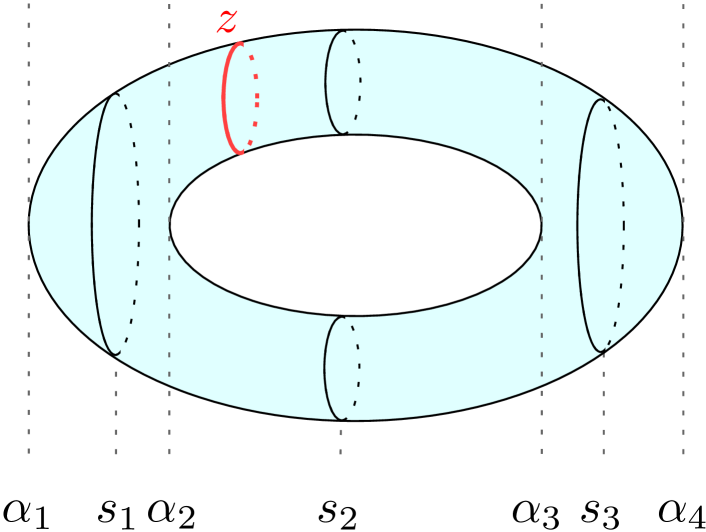
(a) The torus $K$ with the height function $h$ taken over the horizontal line.

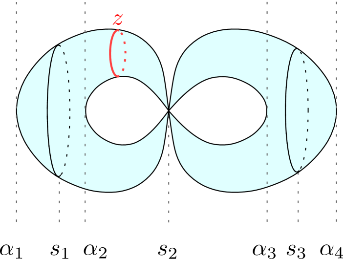
(b) The space $|K|/|K_{4}|$.

$\mathcal{F}$		$K/\mathcal{F}$
$[1,7]^{\text{cc}}_{0}$	$\mapsto$	$[0,0]_{0},[8,8]_{0}$
$[4,4]^{\text{oo}}_{0}$	$\mapsto$	$[0,4]_{1},[4,8]_{1}$
$[2,6]^{\text{oo}}_{1}$	$\mapsto$	$[0,6]_{2},[2,8]_{2}$
$[3,5]^{\text{cc}}_{1}$	$\mapsto$	$[0,2]_{1},[6,8]_{1}$

(c) Interval mapping from $\mathsf{Pers}_{*}(\mathcal{F})$ to $\mathsf{Pers}_{*}(K/\mathcal{F})$.

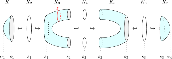
(d) The levelset filtration $\mathcal{F}$ of $h$ which also contains $K_{0}=\varnothing$ and $K_{8}=\varnothing$ at the two ends.

Figure 1: An example for the weak duality of absolute and relative zigzag.

In Figure 1, we provide an example for the duality described above, where we take the height function $h$ on a torus $K$ (Figure 1(a)) and consider the levelset filtration $\mathcal{F}$ [3] of $h$ (Figure 1(d)). We also assume that the torus is finely triangulated. Let $-\infty=\alpha_{0}<\alpha_{1}<\cdots<\alpha_{4}<\alpha_{5}=\infty$ be the critical values of $h$ and $s_{i}$’s be the regular values s.t. $\alpha_{0}<s_{0}<\alpha_{1}<\cdots<\alpha_{4}<s_{4}<\alpha_{5}$. Then, the levelset filtration $\mathcal{F}$ is defined with $h^{-1}(s_{i})$ and $h^{-1}[s_{i},s_{i+1}]$ for the regular values (see [3]). The mapping of intervals from $\mathsf{Pers}_{*}(\mathcal{F})$ to $\mathsf{Pers}_{*}(K/\mathcal{F})$ as in Theorem 6 is listed in Figure 1(c). In Figure 1(c), a superscript ‘cc’ (resp. ‘oo’) indicates that the interval is closed-closed (resp. open-open) and the subscripts denote the dimension of the intervals.

The reason for $[3,5]$ to form a closed-closed interval in $\mathsf{Pers}_{1}(\mathcal{F})$ is that the 1-cycle $z$ is created in $K_{3}$ and its homology class continues to exists in $K_{4}$ and $K_{5}$. To see how a homology class gets born and dies with the corresponding relative intervals, observe that $[z]$ is non-trivial in $\mathsf{H}_{1}(K,K_{0})=\mathsf{H}_{1}(K)$. Also verify that $[z]$ is non-trivial in $\mathsf{H}_{1}(K,K_{1})$ and $\mathsf{H}_{1}(K,K_{2})$. However, $[z]$ becomes trivial in $\mathsf{H}_{1}(K,K_{3})$, $\mathsf{H}_{1}(K,K_{4})$, and $\mathsf{H}_{1}(K,K_{5})$. A quick way to see this is to utilize the fact that $\mathsf{H}_{*}(K,K_{i})\simeq\mathsf{\tilde{H}}_{*}(|K|/|K_{i}|)$ for the good pair $(K,K_{i})$ [13]. For example, we show $|K|/|K_{4}|$ in Figure 1(b), in which $z$ is a trivial 1-cycle. Therefore, $[0,2]$ (and similarly $[6,8]$) forms an interval in $\mathsf{Pers}_{1}(K/\mathcal{F})$ represented by $[z]$.

We can also look at the open-open interval $[2,6]\in\mathsf{Pers}_{1}(\mathcal{F})$, which is represented by the 1-cycle in $K_{2}$ and the homologous cycles in the remaining complexes. Note that this interval $[2,6]$ is actually associated with the only non-trivial class in $\mathsf{H}_{2}(K)$. (Intuitively, one can imagine sweeping the 1-cycle in $K_{2}$ over the horizontal line with proper forking and joining, which would then obtain the entire surface $K$; for more insight into this, we recommend the work [3] and [8].) Describing representatives for the corresponding intervals $[0,6]$ and $[2,8]$ in the relative module is not as straightforward. However, the fact that these two form persistence intervals in $\mathsf{Pers}_{2}(K/\mathcal{F})$ is consistent with the following observation: the 2nd Betti number $\beta_{2}$ of the pairs $(K,K_{0})$, $(K,K_{1})$, $(K,K_{7})$, and $(K,K_{8})$ is 1, whereas $\beta_{2}$ of the remaining pairs from $(K,K_{2})$ to $(K,K_{6})$ is 2 (e.g., there are two 2-cycles in $|K|/|K_{4}|$ in Figure 1(b)). Explicitly listing representatives for the two intervals is beyond the scope of this paper and one can refer to the work [15] and [8] for details.

3.1 Justification

To prove Theorem 6, we draw upon the Diamond Principle proposed by Carlsson and de Silva [2] (see also [3]), which relates the barcodes of two filtrations differing by a local change. We first provide the following definition:

Definition 8 (Mayer-Vietoris diamond [2, 3]).

Two simplex-wise filtrations $\mathcal{F}$ and $\mathcal{F}^{\prime}$ are related by a Mayer-Vietoris diamond if they are of the following forms (where $\sigma\neq\tau$):

(1)

In the above diagram, $\mathcal{F}$ and $\mathcal{F}^{\prime}$ differ only in the complexes at index $j$ and $\mathcal{F}^{\prime}$ is derived from $\mathcal{F}$ by switching the addition of $\sigma$ and deletion of $\tau$. We also say that $\mathcal{F}^{\prime}$ is derived from $\mathcal{F}$ by an outward switch and $\mathcal{F}$ is derived from $\mathcal{F}^{\prime}$ by an inward switch.

Remark 9.

Note that the diagram in Equation (1) is invalid when $\sigma=\tau$. To see this, suppose that the two simplices equal. Then, the fact that $\tau=\sigma$ is deleted from $K_{j-1}$ in $\mathcal{F}^{\prime}$ implies that $\sigma\in K_{j-1}$. This makes $\mathcal{F}$ invalid because we cannot add $\sigma$ to $K_{j-1}$ anymore.

Remark 10.

In Equation (1), we only provide a specific form of Mayer-Vietoris diamond which is sufficient for our purposes; see [2, 3] for a more general form. According to [2], the diamond in Equation (1) is a Mayer-Vietoris diamond because $K_{j}=\linebreak[1]K_{j-1}\cup K_{j+1}$ and $K^{\prime}_{j}=K_{j-1}\cap K_{j+1}$.

We then have the following fact:

Theorem 11 (Diamond Principle [2]).

Given two simplex-wise filtrations $\mathcal{F},\mathcal{F}^{\prime}$ related by a Mayer-Vietoris diamond as in Equation (1), there is a bijection from $\mathsf{Pers}_{*}(\mathcal{F})$ to $\mathsf{Pers}_{*}(\mathcal{F}^{\prime})$ as follows:

$\mathsf{Pers}_{*}(\mathcal{F})$		$\mathsf{Pers}_{*}(\mathcal{F}^{\prime})$
$[b,j-1]$; $b\leq j-1$	$\mapsto$	$[b,j]$
$[b,j]$; $b\leq j-1$	$\mapsto$	$[b,j-1]$
$[j,d]$; $d\geq j+1$	$\mapsto$	$[j+1,d]$
$[j+1,d]$; $d\geq j+1$	$\mapsto$	$[j,d]$
$[j,j]$ of dimension $p$	$\mapsto$	$[j,j]$ of dimension $p-1$
$[b,d]$; all other cases	$\mapsto$	$[b,d]$

Note that the bijection preserves the dimension of the intervals except for $[j,j]$.

Remark 12.

In the above bijection, only an interval containing some but not all of $\{j-1,j,j+1\}$ maps to a different interval or different dimension.

We also observe the following fact which is critical for the proof of Theorem 6:

Proposition 13.

Let $K$ be a simplicial complex and $\mathcal{F}:\varnothing=K_{0}\leftrightarrow K_{1}\leftrightarrow\cdots\leftrightarrow K_{m}=\varnothing$ be a simplex-wise filtration of $K$ which is non-repetitive. Then, there is a simplex-wise up-down filtration

$$\mathcal{U}:\varnothing=L_{0}\hookrightarrow L_{1}\hookrightarrow\cdots\hookrightarrow L_{n}=K\hookleftarrow L_{n+1}\hookleftarrow\cdots\hookleftarrow L_{2n}=\varnothing$$

where $m=2n$ s.t. $\mathcal{F}$ is derived from $\mathcal{U}$ by a sequence of outward switches.

Remark 14.

In Section 5, we further show how an up-down filtration can be converted into a non-zigzag filtration and hence relate the barcode computation for non-repetitive filtrations to the computation of standard persistence.

Proof.

We prove an equivalent statement, i.e., $\mathcal{U}$ is derived from $\mathcal{F}$ by a sequence of inward switches. Suppose that $\mathcal{F}$ is of the form $\mathcal{F}:K_{0}\xleftrightarrow{\;\sigma_{0}\;}K_{1}\xleftrightarrow{\;\sigma_{1}\;}\cdots\xleftrightarrow{\;\sigma_{m-1}\;}K_{m}$. Let $K_{i}\xhookleftarrow{\;\sigma_{i}\;}K_{i+1}$ be the first deletion in $\mathcal{F}$ and $K_{j}\xhookrightarrow{\;\sigma_{j}\;}K_{j+1}$ be the first addition after that. That is, $\mathcal{F}$ is of the form

$$\mathcal{F}:K_{0}\hookrightarrow\cdots\hookrightarrow K_{i}\xhookleftarrow{\;\sigma_{i}\;}K_{i+1}\xhookleftarrow{\;\sigma_{i+1}\;}\cdots\xhookleftarrow{\;\sigma_{j-2}\;}K_{j-1}\xhookleftarrow{\;\sigma_{j-1}\;}K_{j}\xhookrightarrow{\;\sigma_{j}\;}K_{j+1}\leftrightarrow\cdots\leftrightarrow K_{m}$$

Since $\mathcal{F}$ is non-repetitive, we have $\sigma_{j-1}\neq\sigma_{j}$. So we can switch $\xhookleftarrow{\;\sigma_{j-1}\;}$ and $\xhookrightarrow{\;\sigma_{j}\;}$ (which is an inward switch) to derive a filtration

$$K_{0}\hookrightarrow\cdots\hookrightarrow K_{i}\xhookleftarrow{\;\sigma_{i}\;}K_{i+1}\xhookleftarrow{\;\sigma_{i+1}\;}\cdots\xhookleftarrow{\;\sigma_{j-2}\;}K_{j-1}\xhookrightarrow{\;\sigma_{j}\;}K^{\prime}_{j}\xhookleftarrow{\;\sigma_{j-1}\;}K_{j+1}\leftrightarrow\cdots\leftrightarrow K_{m}$$

We then continue performing such inward switches (e.g., the next switch is on $\xhookleftarrow{\;\sigma_{j-2}\;}$ and $\xhookrightarrow{\;\sigma_{j}\;}$) to derive a filtration

$$\mathcal{F}^{\prime}:K_{0}\hookrightarrow\cdots\hookrightarrow K_{i}\xhookrightarrow{\;\sigma_{j}\;}K^{\prime}_{i+1}\xhookleftarrow{\;\sigma_{i}\;}\cdots\xhookleftarrow{\;\sigma_{j-3}\;}K^{\prime}_{j-1}\xhookleftarrow{\;\sigma_{j-2}\;}K^{\prime}_{j}\xhookleftarrow{\;\sigma_{j-1}\;}K_{j+1}\leftrightarrow\cdots\leftrightarrow K_{m}$$

Note that from $\mathcal{F}$ to $\mathcal{F}^{\prime}$, the up-down ‘prefix’ grows longer. We can repeat the above operations on the newly derived $\mathcal{F}^{\prime}$ until the entire filtration turns into an up-down one. ∎

We now prove Theorem 6:

Proof of Theorem 6.

Let $\mathcal{U}:\varnothing=K^{\prime}_{0}\hookrightarrow\cdots\hookrightarrow K^{\prime}_{n}=K\hookleftarrow\cdots\hookleftarrow K^{\prime}_{2n}=\varnothing$ be the simplex-wise, up-down filtration for $\mathcal{F}$ as described in Proposition 13. We first prove that Theorem 6 holds for $\mathcal{U}$. To prove this, we decompose $\mathcal{U}$ into two non-zigzag filtrations $\mathcal{U}_{1},\mathcal{U}_{2}$ sharing the complex $K^{\prime}_{n}=K$ as follows:

Note that we denote $(K,K^{\prime}_{n})$ as $\varnothing$ in $K/\mathcal{U}$ because $\mathsf{H}_{*}(K,K^{\prime}_{n})=0$. We then verify Theorem 6 on $\mathcal{U}$ by utilizing the duality of absolute and relative persistence in the non-zigzag setting [6]. Because of the arrow directions, the birth and death indices of a closed-open interval of $\mathsf{Pers}_{p}(\mathcal{U})$ are also indices for $\mathcal{U}_{1}$. It follows that any closed-open interval $[b,d]\in\mathsf{Pers}_{p}(\mathcal{U})$ is necessarily a finite interval in $\mathsf{Pers}_{p}(\mathcal{U}_{1})$. By the duality for non-zigzag persistence [6], $[b,d]\in\mathsf{Pers}_{p}(\mathcal{U}_{1})$ corresponds to $[b,d]\in\mathsf{Pers}_{p+1}(K/\mathcal{U}_{1})$. Note that $[b,d]\in\mathsf{Pers}_{p+1}(K/\mathcal{U}_{1})$ is also an interval in $\mathsf{Pers}_{p+1}(K/\mathcal{U})$, and hence the correspondence in Theorem 6 is satisfied. Similarly, one can verify the correspondence for open-closed intervals in $\mathsf{Pers}_{p}(\mathcal{U})$, which are necessarily finite intervals in $\mathsf{Pers}_{p}(\mathcal{U}_{2})$. Now let $[b,d]\in\mathsf{Pers}_{p}(\mathcal{U})$ be a closed-closed interval. Then, $b$ and $d$ must be in the indices of $\mathcal{U}_{1}$ and $\mathcal{U}_{2}$ respectively, thus inducing infinite intervals $[b,n]\in\mathsf{Pers}_{p}(\mathcal{U}_{1})$ and $[n,d]\in\mathsf{Pers}_{p}(\mathcal{U}_{2})$. Note that while $\mathcal{U}_{2}$ is a standard (non-zigzag) filtration starting with $K^{\prime}_{2n}=\varnothing$ and growing into $K^{\prime}_{n}=K$, we inherit the indexing from $\mathcal{U}$ for $\mathcal{U}_{2}$ which is thus an indexing in decreasing order. Then, by the duality for non-zigzag persistence [6], $[b,n]\in\mathsf{Pers}_{p}(\mathcal{U}_{1})$ corresponds to $[0,b-1]\in\mathsf{Pers}_{p}(K/\mathcal{U}_{1})$ and $[n,d]\in\mathsf{Pers}_{p}(\mathcal{U}_{2})$ corresponds to $[d+1,2n]\in\mathsf{Pers}_{p}(K/\mathcal{U}_{2})$. This implies the correspondence claimed in Theorem 6. Moreover, the correspondence as we have verified for $\mathsf{Pers}_{*}(\mathcal{U})$ and $\mathsf{Pers}_{*}(K/\mathcal{U})$ is surjective because the correspondence in [6] is surjective. Note that arrow directions in $\mathcal{U}$ disallow any open-open intervals to exist in $\mathsf{Pers}_{*}(\mathcal{U})$. Later in the proof, we will see how open-open intervals are introduced into $\mathsf{Pers}_{*}(\mathcal{F})$.

Next, we prove that the theorem holds for $\mathcal{F}$ by induction. By Proposition 13, $\mathcal{F}$ can be derived from $\mathcal{U}$ by a sequence of outward switches. Then, let $\mathcal{F}^{0}=\mathcal{U},\mathcal{F}^{1},\ldots,\mathcal{F}^{k-1},\mathcal{F}^{k}=\mathcal{F}$ be a sequence of filtrations such that each $\mathcal{F}^{i+1}$ is derived from $\mathcal{F}^{i}$ by an outward switch. Inducting on $i$, we only need to prove that if Theorem 6 holds for $\mathcal{F}^{i}$, then it also holds for $\mathcal{F}^{i+1}$.

Without loss of generality, suppose that $\mathcal{F}^{i}$ and $\mathcal{F}^{i+1}$ are of the following forms:

Note that $K/\mathcal{F}^{i}$ and $K/\mathcal{F}^{i+1}$ are also related by a (general version of) Mayer-Vietoris diamond and the mapping of $\mathsf{Pers}_{*}(K/\mathcal{F}^{i})$ and $\mathsf{Pers}_{*}(K/\mathcal{F}^{i+1})$ is the same as in Theorem 11 (see [3]). Assuming that Theorem 6 holds for $\mathcal{F}^{i}$, we need to verify that the theorem holds for $\mathcal{F}^{i+1}$ under the following cases (recall Remark 3):

1. $L_{j-1}\hookrightarrow L_{j}$ introduces $j$ as a birth index; $L_{j}\hookleftarrow L_{j+1}$ introduces $j+1$ as a birth index.

2. $L_{j-1}\hookrightarrow L_{j}$ introduces $j$ as a birth index; $L_{j}\hookleftarrow L_{j+1}$ introduces $j$ as a death index.

3. $L_{j-1}\hookrightarrow L_{j}$ introduces $j-1$ as a death index; $L_{j}\hookleftarrow L_{j+1}$ introduces $j+1$ as a birth index.

4. $L_{j-1}\hookrightarrow L_{j}$ introduces $j-1$ as a death index; $L_{j}\hookleftarrow L_{j+1}$ introduces $j$ as a death index.

We only verify Case 2 and omit the verification for other cases which is similar. Now suppose that Case 2 happens. We define the following maps:

in which:

• $\phi$ denotes the mapping of intervals from $\mathsf{Pers}_{*}(\mathcal{F}^{i})$ to $\mathsf{Pers}_{*}(K/\mathcal{F}^{i})$ by Theorem 6. Note that for an interval $[b,d]$ in $\mathsf{Pers}_{*}(\mathcal{F}^{i})$, $\phi([b,d])$ is a set of one or two intervals.

• $\psi$ denotes the bijection from $\mathsf{Pers}_{*}(\mathcal{F}^{i})$ to $\mathsf{Pers}_{*}(\mathcal{F}^{i+1})$ and the bijection from $\mathsf{Pers}_{*}(K/\mathcal{F}^{i})$ to $\mathsf{Pers}_{*}(K/\mathcal{F}^{i+1})$ by the Diamond Principle (Theorem 11).

To prove that Theorem 6 holds for $\mathcal{F}^{i+1}$ under Case 2, we show that for any interval $[b,d]$ in $\mathsf{Pers}_{*}(\mathcal{F}^{i})$, the following mappings

satisfy that the interval $\psi([b,d])$ corresponds to the intervals $\psi(\phi([b,d]))$ as claimed in Theorem 6. Therefore, the correspondence in Theorem 6 is verified for $\mathcal{F}^{i+1}$. Furthermore, the above fact implies the following: given that the correspondence for $\mathcal{F}^{i}$ is surjective, the correspondence for $\mathcal{F}^{i+1}$ is also surjective.

For an interval $[b,d]\in\mathsf{Pers}_{*}(\mathcal{F}^{i})$ containing all or none of $\{j-1,j,j+1\}$, we note that intervals in $\phi([b,d])$ also contain all or none of $\{j-1,j,j+1\}$. For example, if $[b,d]$ is a closed-closed interval in $\mathsf{Pers}_{*}(\mathcal{F}^{i})$ s.t. $d<j-1$, then $\phi([b,d])=\{[0,b-1],[d+1,m]\}$, where $[0,b-1]$ contains none of $\{j-1,j,j+1\}$ and $[d+1,m]$ contains all of them. Hence, by Remark 12, $\psi([b,d])=[b,d]$, $\psi(\phi([b,d]))=\phi([b,d])$, and the intervals’ dimensions are preserved. Furthermore, the types (i.e., ‘open’ or ‘closed’) of the two ends of $[b,d]$ do not change from $\mathsf{Pers}_{*}(\mathcal{F}^{i})$ to $\mathsf{Pers}_{*}(\mathcal{F}^{i+1})$. So indeed $\psi(\phi([b,d]))$ are the intervals that $\psi([b,d])$ corresponds to as stated in Theorem 6.

We then show that for any interval in $\mathsf{Pers}_{*}(\mathcal{F}^{i})$ containing some but not all of $\{j-1,j,j+1\}$, the correspondence is still correct after the switch. We have the following two cases:

• First suppose that $[j,j]$ does not form an interval in $\mathsf{Pers}_{*}(\mathcal{F}^{i})$. Then, according to the assumptions in Case 2, the intervals in $\mathsf{Pers}_{*}(\mathcal{F}^{i})$ containing some but not all of $\{j-1,j,j+1\}$ are $[b,j]$ and $[j,d]$, where $b\leq j-1$ and $d\geq j+1$. If $[b,j]$ is a $p$-th closed-closed interval in $\mathsf{Pers}_{*}(\mathcal{F}^{i})$, we have the following mappings:

  where $[0,b-1]$ and $[j,m]$ of dimension $p$ are exactly intervals in $\mathsf{Pers}_{*}(K/\mathcal{F}^{i+1})$ that $[b,j-1]\in\mathsf{Pers}_{p}(\mathcal{F}^{i+1})$ (which is also closed-closed) corresponds to.

  We can similarly verify the correctness of correspondence when $[b,j]\in\mathsf{Pers}_{*}(\mathcal{F}^{i})$ is open-closed (note that $j$ must be a closed death index) and for $[j,d]\in\mathsf{Pers}_{*}(\mathcal{F}^{i})$.

• Now suppose that $[j,j]$ forms a $p$-th interval in $\mathsf{Pers}_{*}(\mathcal{F}^{i})$. Then, again because of the assumptions in Case 2, $[j,j]$ is the only interval in $\mathsf{Pers}_{*}(\mathcal{F}^{i})$ containing some but not all of $\{j-1,j,j+1\}$. Since $[j,j]\in\mathsf{Pers}_{p}(\mathcal{F}^{i})$ is closed-closed, we have the following mappings:

  where $[j,j]$ becomes open-open in $\mathsf{Pers}_{p-1}(\mathcal{F}^{i+1})$ and its correspondence in $\mathsf{Pers}_{*}(K/\mathcal{F}^{i+1})$ illustrated above is exactly as specified in Theorem 6. Notice that the above transition is the only time when open-open intervals are introduced into the absolute modules, given that $\mathsf{Pers}_{*}(\mathcal{U})$ contains no open-open intervals initially. ∎

Remark 15.

The reason why our proof of Theorem 6 does not work for repetitive filtrations is that Proposition 13 does not hold anymore. Suppose that there is a simplex $\sigma$ in $\mathcal{F}$ which is added again after being deleted. Then, the sequence of inward switches used to turn $\mathcal{F}$ into $\mathcal{U}$ in the proof of Proposition 13 must contain a switch of the deletion of $\sigma$ with the addition of $\sigma$, which is invalid due to Remark 9.

4 Codimension-zero and -one zigzag for manifolds

In this section, we first present a near-linear algorithm for computing the $p$-th relative barcode of a zigzag filtration on a $p$-manifold. The algorithm utilizes Lefschetz duality [5, 19] to convert the problem into computing the 0-th barcode of a dual filtration. We then utilize the near-linear algorithm for 0-dimensional zigzag [9] to achieve the time complexity. Assuming further that the filtration is non-repetitive, the weak duality theorem in Section 3 then gives an algorithm for computing the $p$-th barcode and (a subset of) the $(p-1)$-th barcode for the absolute homology in near-linear time.

Throughout the section, we assume the following input:

• $K$ is a simplicial $p$-manifold with $n$ simplices and $\mathcal{F}:\varnothing=K_{0}\xleftrightarrow{\;\sigma_{0}\;}K_{1}\xleftrightarrow{\;\sigma_{1}\;}\cdots\xleftrightarrow{\;\sigma_{m-1}\;}K_{m}=\varnothing$ is a simplex-wise filtration of $K$.

Let $G$ denote the dual graph of $K$, where vertices of $G$ bijectively map to $p$-simplices of $K$ and edges of $G$ bijectively map to $(p-1)$-simplices of $K$. Define a dual filtration $\mathcal{D}:G_{0}\leftrightarrow G_{1}\leftrightarrow\cdots\leftrightarrow G_{m}$, where each $G_{i}$ is a subgraph of $G$ s.t. a vertex (resp. edge) of $G$ is in $G_{i}$ iff its dual $p$-simplex (resp. $(p-1)$-simplex) is not in $K_{i}$. Each $G_{i}$ is a well-defined subgraph because if a $(p-1)$-simplex of $K$ is not in $K_{i}$, all its $p$-cofaces are also not in $K_{i}$. Accordingly, the vertices of each edge of $G_{i}$ are in $G_{i}$. Intuitively, $G_{i}$ encodes the connectivity of $|K|-|K_{i}|$ and an example of $\mathcal{D}$ is given in [9, Section 5] where $\mathbb{R}^{2}$ is viewed as its one-point compactification $\mathbb{S}^{2}$. Note that similarly as in [9, Section 5], inclusion directions in $\mathcal{D}$ are reversed and $\mathcal{D}$ is not necessarily simplex-wise because an arrow may introduce no changes.

We now provide the first conclusion of this section:

Theorem 16.

$\mathsf{Pers}(\mathsf{H}_{p}(K/\mathcal{F}))=\mathsf{Pers}(\mathsf{H}_{0}(\mathcal{D}))$. Hence, $\mathsf{Pers}(\mathsf{H}_{p}(K/\mathcal{F}))$ can be computed with time complexity $O(m\log^{2}n\allowbreak+m\log m)$.

Assuming that $\mathsf{Pers}(\mathsf{H}_{p}(K/\mathcal{F}))=\mathsf{Pers}(\mathsf{H}_{0}(\mathcal{D}))$, we first construct the dual graph $G$ and the dual filtration $\mathcal{D}$ in linear time. After this, we compute $\mathsf{Pers}(\mathsf{H}_{0}(\mathcal{D}))$ using the algorithm in [9]. The time complexity then follows from the time complexity for computing the 0-th barcode [9].

The proof of $\mathsf{Pers}(\mathsf{H}_{p}(K/\mathcal{F}))=\mathsf{Pers}(\mathsf{H}_{0}(\mathcal{D}))$ is by combining the conclusions of Proposition 18, Proposition 19, and Proposition 20. Before presenting the propositions, we first provide the (natural version of) Lefschetz duality [19, $\mathsection$72]:

Theorem 17 (Lefschetz duality).

Let $k$ be an integer s.t. $0\leq k\leq p$. For the complex $K$ (which is a $p$-manifold), one can assign each subcomplex $L$ of $K$ an isomorphism $\lambda_{L}:\mathsf{H}^{k}(K,L)\to\mathsf{H}_{p-k}(|K|-|L|)$. Moreover, the assignment is natural w.r.t. inclusion, i.e., for another subcomplex $L^{\prime}\subseteq L$, the following diagram commutes, where the horizontal maps are induced by inclusion:

Proposition 18.

The following zigzag modules are isomorphic:

which implies that $\mathsf{Pers}(\mathcal{M}_{1})=\mathsf{Pers}(\mathcal{M}_{2})$.

Proof.

The isomorphism between $\mathcal{M}_{1}$ and $\mathsf{H}^{p}(K/\mathcal{F})$ is given by the universal coefficient theorem [13, pg. 196,198], and the isomorphism between $\mathsf{H}^{p}(K/\mathcal{F})$ and $\mathcal{M}_{2}$ is given by the Lefschetz duality (Theorem 17). ∎

Proposition 19.

$\mathsf{Pers}(\mathsf{H}_{p}(K/\mathcal{F}))=\mathsf{Pers}(\mathcal{M}_{1})$.

Proof.

The proof is the same as the proof of Proposition 24 in the full version of [9]. ∎

Proposition 20.

$\mathsf{Pers}(\mathcal{M}_{2})=\mathsf{Pers}(\mathsf{H}_{0}(\mathcal{D}))$.

Proof.

The proof is the same as the proof of Proposition 25 in the full version of [9]. ∎

We now assume that $\mathcal{F}$ is non-repetitive, by which we can draw upon the weak duality theorem in Section 3. Our goal is to (partially) recover intervals for $\mathsf{Pers}(\mathsf{H}_{*}(\mathcal{F}))$ from $\mathsf{Pers}(\mathsf{H}_{p}(K/\mathcal{F}))$ based on the weak duality theorem, so that these intervals for $\mathsf{Pers}(\mathsf{H}_{*}(\mathcal{F}))$ can be computed in near-linear time. Our conclusion is as follows:

Theorem 21.

Suppose that $\mathcal{F}$ is non-repetitive. Given $\mathsf{Pers}(\mathsf{H}_{p}(K/\mathcal{F}))$, one can compute $\mathsf{Pers}(\mathsf{H}_{p}(\mathcal{F}))$, and the closed-open, open-closed, and open-open intervals of $\mathsf{Pers}(\mathsf{H}_{p-1}(\mathcal{F}))$ in linear time. Thus, the above subset of $\mathsf{Pers}(\mathsf{H}_{*}(\mathcal{F}))$ can be computed in $O(m\log^{2}n\allowbreak+m\log m)=O(n\log^{2}n)$ time, where $m=2n$.

Remark 22.

The subset of $\mathsf{Pers}(\mathsf{H}_{*}(\mathcal{F}))$ that we can recover contain all those intervals derived from pairings involving $p$-simplices. For example, an open-open interval of $\mathsf{Pers}(\mathsf{H}_{p-1}(\mathcal{F}))$ is produced by pairing the deletion of a $p$-simplex with the addition of another $p$-simplex.

Proof $($Sketch$)$.

(See Appendix A for the complete proof.) By the weak duality theorem, we can directly recover all closed-open and open-closed intervals in $\mathsf{Pers}(\mathsf{H}_{p-1}(\mathcal{F}))$ from $\mathsf{Pers}(\mathsf{H}_{p}(K/\mathcal{F}))$. To pair an interval $[0,d]\in\mathsf{Pers}_{p}(K/\mathcal{F})$ with an interval $[b,m]\in\mathsf{Pers}_{p}(K/\mathcal{F})$ (see the discussions after Theorem 6 in Section 3), we note that the destroyer $\sigma_{d}$ of $[0,d]$ and the creator $\sigma_{b-1}$ of $[b,m]$ (see Definition 25) must come from the same connected component of $K$. Also, there is exactly one interval in $\mathsf{Pers}_{p}(K/\mathcal{F})$ with birth at $0$ (death at $m$ resp.) per component of $K$ because $\mathsf{H}_{p}(K,K_{0})=\mathsf{H}_{p}(K)=\mathsf{H}_{p}(K,K_{m})$ has dimension equal to the number of components in $K$. We can then recover closed-closed intervals in $\mathsf{Pers}(\mathsf{H}_{p}(\mathcal{F}))$ and open-open intervals in $\mathsf{Pers}(\mathsf{H}_{p-1}(\mathcal{F}))$. Note that $\mathsf{Pers}(\mathsf{H}_{p}(\mathcal{F}))$ contains only closed-closed intervals. ∎

5 Non-repetitive zigzag via standard persistence

Proposition 13 presented in Section 3 indicates that a non-repetitive filtration admits an up-down filtration as its ‘canonical’ form. In this section, utilizing this canonical form, we show that computing absolute barcodes (and hence relative barcodes by duality) for non-repetitive zigzag filtrations can be reduced to computing barcodes for certain non-zigzag filtrations. This finding leads to a more efficient persistence algorithm for non-repetitive zigzag filtrations considering that standard (non-zigzag) persistence admits faster algorithms [1, 4, 6] in practice, which we confirm with our experiments. Furthermore, the finding locates instances of zigzag filtrations which make the barcode computation far more slower than the non-zigzag ones. These filtrations are those where simplices are repeatedly added and deleted.

Throughout the section, suppose that we are given a non-repetitive, simplex-wise filtration

$$\mathcal{F}:\varnothing=K_{0}\xleftrightarrow{\;\sigma_{0}\;}K_{1}\xleftrightarrow{\;\sigma_{1}\;}\cdots\xleftrightarrow{\;\sigma_{m-1}\;}K_{m}=\varnothing$$

of a complex $K$. Then, let

$$\mathcal{U}:\varnothing=L_{0}\xhookrightarrow{\;\tau_{0}\;}\cdots\xhookrightarrow{\;\tau_{n-1}\;}L_{n}=K\xhookleftarrow{\;\tau_{n}\;}\cdots\xhookleftarrow{\;\tau_{2n-1}\;}L_{2n}=\varnothing$$

be the up-down filtration for $\mathcal{F}$ as described in Proposition 13, where $m=2n$. Utilizing Proposition 13 and the Diamond Principle (Theorem 11), we first relate intervals of $\mathsf{Pers}_{*}(\mathcal{F})$ to intervals of $\mathsf{Pers}_{*}(\mathcal{U})$. Then, we relate $\mathsf{Pers}_{*}(\mathcal{U})$ to the barcode of an extended persistence [5] filtration and draw upon the efficient algorithms for non-zigzag persistence [1, 4, 6].

In summary, our main tasks are:

• Convert the given non-repetitive filtration to an up-down filtration.

• Convert the up-down filtration to a non-zigzag filtration with the help of an extended persistence filtration and compute the standard persistence barcode.

• Convert the standard persistence barcode to the barcode of the input filtration based on rules given in Proposition 28 and 31.

5.1 Conversion to up-down filtration

In a simplex-wise zigzag filtration, for a simplex $\sigma$, let its addition be denoted as $\mathsf{a}\sigma$ and its deletion be denoted as $\mathsf{d}\sigma$. From the proof of Proposition 13, we observe the following: during the transition from $\mathcal{F}$ to $\mathcal{U}$, for any two additions $\mathsf{a}\sigma$, $\mathsf{a}\sigma^{\prime}$ in $\mathcal{F}$ (and similarly for deletions), if $\mathsf{a}\sigma$ is before $\mathsf{a}\sigma^{\prime}$ in $\mathcal{F}$, then $\mathsf{a}\sigma$ is also before $\mathsf{a}\sigma^{\prime}$ in $\mathcal{U}$. We then have the following fact:

Fact 23.

Given the filtration $\mathcal{F}$, to derive $\mathcal{U}$, one only needs to scan $\mathcal{F}$ and list all the additions first and then the deletions, following the order in $\mathcal{F}$.

Remark 24.

Figure 2 gives an example of $\mathcal{F}$ and its corresponding $\mathcal{U}$, where the additions and deletions in $\mathcal{F}$ and $\mathcal{U}$ follow the same order.

Definition 25 (Creator and destroyer).

For any interval $[b,d]\in\mathsf{Pers}_{*}(\mathcal{F})$, if $K_{b-1}\xleftrightarrow{\;\sigma_{b-1}\;}K_{b}$ is forward (resp. backward), we call $\mathsf{a}\sigma_{b-1}$ (resp. $\mathsf{d}\sigma_{b-1}$) the creator of $[b,d]$. Similarly, if $K_{d}\xleftrightarrow{\;\sigma_{d}\;}K_{d+1}$ is forward (resp. backward), we call $\mathsf{a}\sigma_{d}$ (resp. $\mathsf{d}\sigma_{d}$) the destroyer of $[b,d]$.

By inspecting the interval mapping in the Diamond Principle, we have the following fact:

Proposition 26.

For two simplex-wise filtrations $\mathcal{L},\mathcal{L}^{\prime}$ related by a Mayer-Vietoris diamond, any two intervals of $\mathsf{Pers}_{*}(\mathcal{L})$ and $\mathsf{Pers}_{*}(\mathcal{L}^{\prime})$ mapped by the Diamond Principle have the same set of creator and destroyer, though the creator and destroyer may swap. This implies that there is a bijection from $\mathsf{Pers}_{*}(\mathcal{U})$ to $\mathsf{Pers}_{*}(\mathcal{F})$ s.t. any two corresponding intervals have the same set of creator and destroyer.

Remark 27.

The only time when the creator and destroyer swap in a Mayer-Vietoris diamond is when the interval $[j,j]$ for the upper filtration in Equation (1) turns into the same interval (of one dimension lower) for the lower filtration.

Consider the example in Figure 2 for an illustration of Proposition 26. In the example, $[1,2]\in\mathsf{Pers}_{1}(\mathcal{F})$ corresponds to $[1,4]\in\mathsf{Pers}_{1}(\mathcal{U})$, where their creator is $\mathsf{a}\{a,d\}$ and their destroyer is $\mathsf{d}\{a,b\}$. Moreover, $[4,6]\in\mathsf{Pers}_{0}(\mathcal{F})$ corresponds to $[4,5]\in\mathsf{Pers}_{1}(\mathcal{U})$. The creator of $[4,6]\in\mathsf{Pers}_{0}(\mathcal{F})$ is $\mathsf{d}\{b,d\}$ and the destroyer is $\mathsf{a}\{b,c\}$. Meanwhile, $[4,5]\in\mathsf{Pers}_{1}(\mathcal{U})$ has the same set of creator and destroyer but the roles swap.

Figure 2: A non-repetitive filtration $\mathcal{F}$ and its corresponding up-down filtration $\mathcal{U}$. For brevity, $\mathcal{F}$ does not start and end with empty complexes (which can be treated as a truncated case).

For any $\mathsf{a}\sigma$ or $\mathsf{d}\sigma$ in $\mathcal{F}$, let $\mathtt{id}_{\mathcal{F}}(\mathsf{a}\sigma)$ or $\mathtt{id}_{\mathcal{F}}(\mathsf{d}\sigma)$ denote the index (position) of the addition or deletion. For example, for an addition $K_{i}\xhookrightarrow{\;\sigma_{i}\;}K_{i+1}$ in $\mathcal{F}$, $\mathtt{id}_{\mathcal{F}}(\mathsf{a}\sigma_{i})=i$. Proposition 26 indicates the following explicit mapping from $\mathsf{Pers}_{*}(\mathcal{U})$ to $\mathsf{Pers}_{*}(\mathcal{F})$:

Proposition 28.

There is a bijection from $\mathsf{Pers}_{*}(\mathcal{U})$ to $\mathsf{Pers}_{*}(\mathcal{F})$ which maps each $[b,d]\in\mathsf{Pers}_{p}(\mathcal{U})$ by the following rule:

Type	Condition		Type	Interval in $\mathsf{Pers}_{*}(\mathcal{F})$	Dim
closed-open	-	$\mapsto$	closed-open	$\big{[}\mathtt{id}_{\mathcal{F}}(\mathsf{a}\tau_{b-1})+1,\mathtt{id}_{\mathcal{F}}({\mathsf{a}\tau_{d}})\big{]}$	$p$
open-closed	-	$\mapsto$	open-closed	$\big{[}\mathtt{id}_{\mathcal{F}}(\mathsf{d}\tau_{b-1})+1,\mathtt{id}_{\mathcal{F}}({\mathsf{d}\tau_{d}})\big{]}$	$p$
closed-closed	$\mathtt{id}_{\mathcal{F}}(\mathsf{a}\tau_{b-1})<\mathtt{id}_{\mathcal{F}}({\mathsf{d}\tau_{d}})$	$\mapsto$	closed-closed	$\big{[}\mathtt{id}_{\mathcal{F}}(\mathsf{a}\tau_{b-1})+1,\mathtt{id}_{\mathcal{F}}({\mathsf{d}\tau_{d}})\big{]}$	$p$
	$\mathtt{id}_{\mathcal{F}}(\mathsf{a}\tau_{b-1})>\mathtt{id}_{\mathcal{F}}({\mathsf{d}\tau_{d}})$	$\mapsto$	open-open	$\big{[}\mathtt{id}_{\mathcal{F}}({\mathsf{d}\tau_{d}})+1,\mathtt{id}_{\mathcal{F}}(\mathsf{a}\tau_{b-1})\big{]}$	$p-1$

Remark 29.

As mentioned in the proof of Theorem 6, $\mathsf{Pers}_{*}(\mathcal{U})$ contains no open-open intervals. However, a closed-closed interval $[b,d]\in\mathsf{Pers}_{p}(\mathcal{U})$ turns into an open-open interval in $\mathsf{Pers}_{p-1}(\mathcal{F})$ when $\mathtt{id}_{\mathcal{F}}(\mathsf{a}\tau_{b-1})>\mathtt{id}_{\mathcal{F}}({\mathsf{d}\tau_{d}})$. The type of such a closed-closed interval changes when it turns into a single point interval $[j,j]$ during the sequence of outward switches, after which the closed-closed interval $[j,j]$ becomes an open-open interval $[j,j]$ with a dimension shift (see Theorem 11).

We can take the example in Figure 2 for the mapping in Proposition 28. The interval $[4,5]\in\mathsf{Pers}_{1}(\mathcal{U})$ is a closed-closed one whose creator is $\mathsf{a}\{b,c\}$ and destroyer is $\mathsf{d}\{b,d\}$. We have that $\mathtt{id}_{\mathcal{F}}(\mathsf{a}\{b,c\})=6>\mathtt{id}_{\mathcal{F}}(\mathsf{d}\{b,d\})=3$, so that the corresponding interval in $\mathsf{Pers}_{0}(\mathcal{F})$ is

$$[\mathtt{id}_{\mathcal{F}}(\mathsf{d}\{b,d\})+1,\mathtt{id}_{\mathcal{F}}(\mathsf{a}\{b,c\})]=[4,6]$$

5.2 Conversion to non-zigzag filtration

We first convert the up-down filtration $\mathcal{U}$ to an extended persistence [5] filtration $\mathcal{E}$ which is then easily converted to an (absolute) non-zigzag filtration using the ‘coning’ technique [5].

Inspired by the Mayer-Vietoris pyramid in [3], we relate $\mathsf{Pers}_{*}(\mathcal{U})$ to the barcode of the filtration $\mathcal{E}$ defined as:

$$\mathcal{E}:\varnothing=L_{0}\hookrightarrow\cdots\hookrightarrow L_{n}=(K,L_{2n})\hookrightarrow(K,L_{2n-1})\hookrightarrow\cdots\hookrightarrow(K,L_{n})=(K,K)$$

where $L_{n}=K=(K,L_{2n}=\varnothing)$. When denoting the persistence intervals of $\mathcal{E}$, we let the increasing index for the first half of $\mathcal{E}$ continue to the second half, i.e., $(K,L_{2n-1})$ has index $n+1$ and $(K,L_{n})$ has index $2n$. Then, it can be verified that an interval $[b,d]\in\mathsf{Pers}_{*}(\mathcal{E})$ for $b<n<d$ starts with the complex $L_{b}$ and ends with $(K,L_{3n-d})$.

Remark 30.

A filtration in extended persistence [5] is originally defined for a PL function $f$, where the first half is the lower-star filtration of $f$ and the second half (the relative part) is derived from the upper-star filtration of $f$. The filtration $\mathcal{E}$ defined above is a generalization of the one in [5].

Proposition 31.

There is a bijection from $\mathsf{Pers}_{*}(\mathcal{E})$ to $\mathsf{Pers}_{*}(\mathcal{U})$ which maps each $[b,d]\in\mathsf{Pers}_{*}(\mathcal{E})$ of dimension $p$ by the following rule:

Type	Condition		Type	Interv. in $\mathsf{Pers}_{*}(\mathcal{U})$	Dim
Ord	$d<n$	$\mapsto$	closed-open	$[b,d]$	$p$
Rel	$b>n$	$\mapsto$	open-closed	$[3n-d,3n-b]$	$p-1$
Ext	$b\leq n\leq d$	$\mapsto$	closed-closed	$[b,3n-d-1]$	$p$

Remark 32.

The types ‘Ord’, ‘Rel’, and ‘Ext’ for intervals in $\mathsf{Pers}_{*}(\mathcal{E})$ are as defined in [5], which stand for intervals from the ordinary sub-barcode, the relative sub-barcode, and the extended sub-barcode.

Figure 3: A Mayer-Vietoris pyramid relating the second half of $\mathcal{E}$ and $\mathcal{U}$ for $n=4$.

Proof $($Sketch$)$.

We can build a Mayer-Vietoris pyramid relating the second half of $\mathcal{E}$ and the second half of $\mathcal{U}$ similar to the one in [3]. A pyramid for $n=4$ is shown in Figure 3, where the second half of $\mathcal{E}$ is along the left side of the triangle and the second half of $\mathcal{U}$ is along the bottom. In Figure 3, we represent the second half of $\mathcal{E}$ and $\mathcal{U}$ in a slightly different way considering that $L_{4}=K$ and $L_{8}=\varnothing$. Also, each vertical arrow indicates the addition of a simplex in the second complex of the pair and each horizontal arrow indicates the deletion of a simplex in the first complex.

To see the correctness of the mapping, we first note that each square in the pyramid is a Mayer-Vietoris diamond. Then, the mapping as stated can be verified using the Diamond Principle (Theorem 11). However, there is a quicker way to verify the mapping in the proposition by observing the following: corresponding intervals in $\mathsf{Pers}_{*}(\mathcal{E})$ and $\mathsf{Pers}_{*}(\mathcal{U})$ have the same set of creator and destroyer if we ignore whether it is the addition or deletion of a simplex. For example, an interval in $\mathsf{Pers}_{*}(\mathcal{E})$ may be created by the addition of a simplex $\sigma$ in the first half of $\mathcal{E}$ and destroyed by the addition of another simplex $\sigma^{\prime}$ in the second half of $\mathcal{E}$. Then, its corresponding interval in $\mathsf{Pers}_{*}(\mathcal{U})$ is also created by the addition of $\sigma$ in the first half but destroyed by the deletion of $\sigma^{\prime}$ in the second half. Note that the dimension change for the case $b>n$ is caused by the swap of creator and destroyer. ∎

By Proposition 28 and 31, we only need to compute $\mathsf{Pers}_{*}(\mathcal{E})$ in order to compute $\mathsf{Pers}_{*}(\mathcal{F})$. The barcode of $\mathcal{E}$ can be computed using the ‘coning’ technique [5], which converts $\mathcal{E}$ into an (absolute) non-zigzag filtration $\hat{\mathcal{E}}$. Specifically, let $\omega$ be a vertex different from all vertices in $K$. The cone $\omega\cdot\sigma$ of a simplex $\sigma$ of $K$ is the simplex $\sigma\cup\{\omega\}$. The cone $\omega\cdot L_{i}$ of a complex $L_{i}$ consists of three parts: the vertex $\omega$, $L_{i}$, and cones of all simplices of $L_{i}$. The filtration $\hat{\mathcal{E}}$ is then defined as [5]:

$$\hat{\mathcal{E}}:L_{0}\cup\{\omega\}\hookrightarrow\cdots\hookrightarrow L_{n}\cup\{\omega\}=K\cup\omega\cdot L_{2n}\hookrightarrow K\cup\omega\cdot L_{2n-1}\hookrightarrow\cdots\hookrightarrow K\cup\omega\cdot L_{n}$$

We have that $\mathsf{Pers}_{*}(\mathcal{E})$ equals $\mathsf{Pers}_{*}(\hat{\mathcal{E}})$ without the only infinite interval [5]. Note that if a simplex $\sigma$ is added (to the second complex) from $(K,L_{i})$ to $(K,L_{i-1})$ in $\mathcal{E}$, then the cone $\omega\cdot\sigma$ is added from $K\cup\omega\cdot L_{i}$ to $K\cup\omega\cdot L_{i-1}$ in $\hat{\mathcal{E}}$.

We now have the conclusion of this section:

Theorem 33.

The barcode of a non-repetitive, simplex-wise zigzag filtration with length $m$ can be computed in time $T(m)+O(m)$, where $T(m)$ is the time used for computing the barcode of a non-zigzag filtration with length $m$.

Proof.

Given an input $\mathcal{F}$, we first construct the filtration $\mathcal{U}$, the map $\mathtt{id}_{\mathcal{F}}$, and the filtration $\hat{\mathcal{E}}$ in linear time. After running a non-zigzag persistence algorithm on $\hat{\mathcal{E}}$, we can derive $\mathsf{Pers}_{*}(\mathcal{F})$ by the mappings in Proposition 28 and 31, in linear time. ∎

5.3 Experiments

We implemented our algorithm for non-repetitive filtrations described in this section and compared the performance with Dionysus [17] and Dionysus2 [18], which are two versions of implementation of the zigzag persistence algorithm (for general filtrations) described in [3]. In our implementation, we utilize the Simpers [7] software for the computation of non-zigzag persistence.

To generate non-repetitive filtrations, we first take a simplicial complex with vertices in $\mathbb{R}^{3}$, and then take the height function $h$ along a certain axis on the complex. After this, we build an up-down filtration for the complex where the first half is the lower-star filtration of $h$ and the second half is the (reversed) upper-star filtration of $h$. We then randomly perform outward switches on the up-down filtration to derive a non-repetitive filtration. Note that the simplicial complex is derived from a triangular mesh with a Vietoris-Rips complex on the vertices as a supplement.

Table 1 lists the running time of the three algorithms on various non-repetitive filtrations we generate. The column ‘Mesh’ contains the triangular mesh used to generate each filtration; the column ‘Length’ contains the length (i.e., number of additions and deletions) of each filtration; the columns ‘$\text{T}_{\text{ours}}$’, ‘$\text{T}_{\text{Dio}}$’, and ‘$\text{T}_{\text{Dio2}}$’ contain the running time of our algorithm, Dionysus, and Dionysus2 respectively; the column ‘Speedup’ equals $\min(\text{T}_{\text{Dio}},\text{T}_{\text{Dio2}})/\text{T}_{\text{ours}}$. From the table, the speedup of our algorithm is significant: on inputs with about 5 million of additions and deletions, our algorithm is 50 or 100 times faster than the other two algorithms. This speedup is expected as our algorithm only needs a slight amount of additional processing other than the non-zigzag persistence computation. Note that the newer version Dionysus2 is not always faster than its older version (i.e., on the filtration of Dragon). Hence, for a conservative estimate, we took the best performer of the two versions for comparing with our algorithm.

Table 1: Running time of our algorithm, Dionysus, and Dionysus2 on non-repetitive filtrations. All tests were run on a commodity MacBook Pro with a 3.1GHz Dual-Core CPU and 8GB memory.

Mesh	Length	$\text{T}_{\text{ours}}$	$\text{T}_{\text{Dio}}$	$\text{T}_{\text{Dio2}}$	Speedup
Bunny	419,372	2.9s	46.6s	26.4s	9.1
Armadillo	2,075,680	14.8s	17m27.3s	8m41.6s	35.2
Hand	5,254,620	44.6s	39m38.2s	23m59.0s	53.3
Dragon	5,260,700	42.6s	1h11m52.5s	1h53m33.2s	101.2

6 Conclusions

In this paper, we study one of the two types of dualities for persistence [5, 6] in the zigzag setting, which is the duality for the absolute and relative zigzag modules. The other duality for persistent homology and cohomology addressed in [6] can be adapted to the zigzag setting straightforwardly; see [9, Section 5]. Furthermore, the weak duality result presented in Theorem 6 extends to cohomology modules directly due to the equivalence of barcodes for zigzag persistent homology and cohomology.

Our main finding is a weak duality result for the absolute and relative zigzag modules generated from non-repetitive filtrations. This weak duality led to two efficient algorithms for non-repetitive filtrations, one for manifolds and the other in general. Naturally, it raises the question if a similar result exists for repetitive filtrations.

We have shown that computing zigzag persistence for non-repetitive filtrations is almost as efficient as computing standard persistence. However, for zigzag filtrations in general, the persistence computation [3, 15] is still far more costly than standard persistence (though theoretically the time complexities are the same [16]). This research motivates the question if further insights into zigzag persistence can lead to computing general zigzag persistence more efficiently in practice.

Appendix A Proof of Theorem 21

For the proof, in Table 2, we rewrite the correspondence in Theorem 6. We then have the following:

Table 2: The correspondence of intervals in Theorem 6 rewritten for the proof of Theorem 21.

$\mathsf{Pers}(\mathsf{H}_{*}(\mathcal{F}))$				$\mathsf{Pers}(\mathsf{H}_{p}(K/\mathcal{F}))$
Type	Interval	Dim		Interval(s)
closed-open, open-closed	$[b,d]$	$p-1$	$\mapsto$	$[b,d]$
closed-closed	$[b,d]$	$p$	$\mapsto$	$[0,b-1]$, $[d+1,m]$
open-open	$[b,d]$	$p-1$	$\mapsto$	$[0,d]$, $[b,m]$

• There is an identity map from closed-open and open-closed intervals in $\mathsf{Pers}(\mathsf{H}_{p-1}(\mathcal{F}))$ to intervals in $\mathsf{Pers}(\mathsf{H}_{p}(K/\mathcal{F}))$ which does not start with $0$ and does not end with $m$. The reason is that all intervals in $\mathsf{Pers}(\mathsf{H}_{p}(K/\mathcal{F}))$ which are correspondence of closed-closed or open-open intervals in $\mathsf{Pers}(\mathsf{H}_{*}(\mathcal{F}))$ either starts with $0$ or ends with $m$. Therefore, from $\mathsf{Pers}(\mathsf{H}_{p}(K/\mathcal{F}))$, one can recover closed-open and open-closed intervals in $\mathsf{Pers}(\mathsf{H}_{p-1}(\mathcal{F}))$ in linear time.

• There is an even number of intervals in $\mathsf{Pers}(\mathsf{H}_{p}(K/\mathcal{F}))$ starting with $0$ or ending with $m$. Furthermore, these intervals form a pairing such that each pair comes from a closed-closed or open-open interval in $\mathsf{Pers}(\mathsf{H}_{*}(\mathcal{F}))$ as shown in Table 2. Let $[0,i]$ and $[j,m]$ be such a pair. By inspecting Table 2, we notice that $i$ must be an open death index and $j$ must be an open birth index. It follows that the interval $[0,i]$ ends because of the addition of the $p$-simplex $\sigma_{i}$ and the interval $[j,m]$ starts because of the deletion of the $p$-simplex $\sigma_{j-1}$. We have the following cases:

  • $i<j$: In this case, $[0,i]$ and $[j,m]$ are disjoint, which means that they must come from the closed-closed interval $[i+1,j-1]\in\mathsf{Pers}(\mathsf{H}_{p}(\mathcal{F}))$ as in Table 2. Notice that $[i+1,j-1]$ starts because of the addition of $\sigma_{i}$ and ends because of the deletion of $\sigma_{j-1}$. Since indeed the zigzag persistence of $\mathcal{F}$ can be independently defined on each connected component of $K$, we must have that $\sigma_{i}$ and $\sigma_{j-1}$ come from the same connected component of $K$.

  • $i\geq j$: In this case, $[0,i]$ intersects $[j,m]$, which means that they must come from the open-open interval $[j,i]\in\mathsf{Pers}(\mathsf{H}_{p-1}(\mathcal{F}))$. Notice that $[j,i]$ starts because of the deletion of $\sigma_{j-1}$ and ends because of the addition of $\sigma_{i}$. Then similarly as for the previous case, $\sigma_{i}$ and $\sigma_{j-1}$ must come from the same connected component of $K$.

  From the above observations, in order to recover the closed-closed intervals in $\mathsf{Pers}(\mathsf{H}_{p}(\mathcal{F}))$ and the open-open intervals in $\mathsf{Pers}(\mathsf{H}_{p-1}(\mathcal{F}))$, one only needs to do the following, which can be done in linear time:

  • For each interval $[0,i]\in\mathsf{Pers}(\mathsf{H}_{p}(K/\mathcal{F}))$, take the $p$-simplex $\sigma_{i}$, and for each interval $[j,m]\in\mathsf{Pers}(\mathsf{H}_{p}(K/\mathcal{F}))$, take the $p$-simplex $\sigma_{j-1}$. Pair all the $\sigma_{i}$’s and $\sigma_{j-1}$’s (and hence their corresponding intervals) belonging to the same connected component of $K$. Note that the pairing is unique because closed-closed intervals in $\mathsf{Pers}(\mathsf{H}_{p}(\mathcal{F}))$ and open-open intervals in $\mathsf{Pers}(\mathsf{H}_{p-1}(\mathcal{F}))$ bijectively map to the basis of $\mathsf{H}_{p}(K)$ and hence bijectively map to the components of $K$ (this can be seen from the proof of Theorem 6).

  • For each pair $[0,i]$ and $[j,m]$ in the previous step, if $i<j$, then we have a closed-closed interval $[i+1,j-1]\in\mathsf{Pers}(\mathsf{H}_{p}(\mathcal{F}))$; otherwise, we have an open-open interval $[j,i]\in\mathsf{Pers}(\mathsf{H}_{p-1}(\mathcal{F}))$.

One final thing we need to verify is that $\mathsf{Pers}(\mathsf{H}_{p}(\mathcal{F}))$ contains only closed-closed intervals, which follows from the fact that $K$ contains no $(p+1)$-simplices.

References

- [1] Jean-Daniel Boissonnat, Tamal K. Dey, and Clément Maria. The compressed annotation matrix: An efficient data structure for computing persistent cohomology. Algorithmica, 73(3):607–619, 2015.
- [2] Gunnar Carlsson and Vin de Silva. Zigzag persistence. Foundations of Computational Mathematics, 10(4):367–405, 2010.
- [3] Gunnar Carlsson, Vin de Silva, and Dmitriy Morozov. Zigzag persistent homology and real-valued functions. In Proceedings of the Twenty-Fifth Annual Symposium on Computational Geometry, pages 247–256, 2009.
- [4] Chao Chen and Michael Kerber. An output-sensitive algorithm for persistent homology. Comput. Geom.: Theory and Applications, 46(4):435–447, 2013.
- [5] David Cohen-Steiner, Herbert Edelsbrunner, and John Harer. Extending persistence using Poincaré and Lefschetz duality. Foundations of Computational Mathematics, 9(1):79–103, 2009.
- [6] Vin de Silva, Dmitriy Morozov, and Mikael Vejdemo-Johansson. Dualities in persistent (co)homology. Inverse Problems, 27(12):124003, 2011.
- [7] Tamal K. Dey, Fengtao Fan, and Yusu Wang. Computing topological persistence for simplicial maps. In Proceedings of the Thirtieth Annual Symposium on Computational Geometry, pages 345–354, 2014.
- [8] Tamal K. Dey and Tao Hou. Computing optimal persistent cycles for levelset zigzag on manifold-like complexes. arXiv preprint arXiv:2105.00518, 2021.
- [9] Tamal K. Dey and Tao Hou. Computing zigzag persistence on graphs in near-linear time. In 37th International Symposium on Computational Geometry, SoCG 2021, volume 189 of LIPIcs, pages 30:1–30:15. Schloss Dagstuhl - Leibniz-Zentrum für Informatik, 2021.
- [10] Tamal K. Dey, Marian Mrozek, and Ryan Slechta. Persistence of the conley index in combinatorial dynamical systems. In 36th International Symposium on Computational Geometry (SoCG 2020). Schloss Dagstuhl-Leibniz-Zentrum für Informatik, 2020.
- [11] Herbert Edelsbrunner, David Letscher, and Afra Zomorodian. Topological persistence and simplification. In Proceedings 41st Annual Symposium on Foundations of Computer Science, pages 454–463. IEEE, 2000.
- [12] Peter Gabriel. Unzerlegbare Darstellungen I. Manuscripta Mathematica, 6(1):71–103, 1972.
- [13] Allen Hatcher. Algebraic Topology. Cambridge University Press, 2002.
- [14] Petter Holme and Jari Saramäki. Temporal networks. Physics Reports, 519(3):97–125, 2012.
- [15] Clément Maria and Steve Y. Oudot. Zigzag persistence via reflections and transpositions. In Proceedings of the Twenty-Sixth Annual ACM-SIAM Symposium on Discrete Algorithms, pages 181–199. SIAM, 2014.
- [16] Nikola Milosavljević, Dmitriy Morozov, and Primoz Skraba. Zigzag persistent homology in matrix multiplication time. In Proceedings of the Twenty-Seventh Annual Symposium on Computational Geometry, pages 216–225, 2011.
- [17] Dmitriy Morozov. Dionysus. URL: https://www.mrzv.org/software/dionysus/.
- [18] Dmitriy Morozov. Dionysus2. URL: https://www.mrzv.org/software/dionysus2/.
- [19] James R. Munkres. Elements of Algebraic Topology. CRC Press, 2018.
- [20] Afra Zomorodian and Gunnar Carlsson. Computing persistent homology. Discrete & Computational Geometry, 33(2):249–274, 2005.