LiST: Lite Prompted Self-training Makes Parameter-efficient
Few-shot Learners

Abstract

We present a new method LiST for parameter-efficient fine-tuning of large pre-trained language models (PLMs) for few-shot learning. LiST improves over recent methods that adopt prompt-based fine-tuning (FN) using two key techniques. The first is the use of self-training to leverage large amounts of unlabeled data for prompt-based FN in few-shot settings. We use self-training in conjunction with meta-learning for re-weighting noisy pseudo-prompt labels. Self-training is expensive as it requires updating all the model parameters repetitively. Therefore, we use a second technique for light-weight fine-tuning where we introduce a small number of task-specific parameters that are fine-tuned during self-training while keeping the PLM encoder frozen. Our experiments show that LiST can effectively leverage unlabeled data to improve the model performance for few-shot learning. Additionally, the fine-tuning is efficient as it only updates a small percentage of parameters and the overall model footprint is reduced since several tasks can share a common PLM encoder as backbone. A comprehensive study on six NLU tasks demonstrate LiST to improve by $35\%$ over classic fine-tuning and $6\%$ over prompt-based FN with $96\%$ reduction in number of trainable parameters when fine-tuned with no more than $30$ labeled examples from each task. With only $14M$ tunable parameters, LiST outperforms GPT-3 in-context learning by $33\%$ on few-shot NLU tasks.

1 Introduction

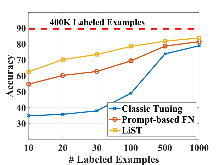
(a) Performance Comparison

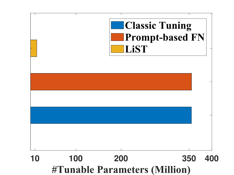
(b) Tunable Parameters

Figure 1: LiST leverages prompt-based fine-tuning (FN) with unlabeled data for label-efficiency and adapters for reducing tunable parameters. (a) shows classic tuning, prompt-based FN and LiST using RoBERTa-large as backbone on MNLI task for a comparison. The red dash line depicts ceiling performance with full supervision with RoBERTa-large. (b) shows the number of tunable parameters for each method. Table 2 shows a comparison with GPT-3 in-context learning.

Large pre-trained language models (PLMs) have obtained state-of-the-art performance in several natural language understanding tasks (Devlin et al., 2019a; Clark et al., 2020; Liu et al., 2019a). Despite their remarkable success in fully supervised settings, their performance is still not satisfactory when fine-tuning with only a handful of labeled examples. While models like GPT-3 (Brown et al., 2020) have obtained impressive few-shot performance with in-context task adaptation, they have a significant performance gap relative to fully supervised SoTA models. For instance, few-shot GPT-3 performance is $20$ points worse than fully-tuned DeBERTa (He et al., 2021) on SuperGLUE. This poses significant challenges for many real-world tasks where large labeled data is difficult to obtain.

In this work, we present a new fine-tuning method LiST that aims to improve few-shot learning ability over existing fine-tuning strategies using two techniques as follows.

The first one is to leverage self-training with large amounts of unlabeled data from the target domain to improve model adaptation in few-shot settings. Prompt-based fine-tuning (Gao et al., 2021) have recently shown significant improvements over classic fine-tuning in the few-shot learning setting. In this paper, we demonstrate that self-training with unlabeled data is able to significantly improve prompt-based fine-tuning (Gao et al., 2021) where we iteratively update a pair of teacher and student models given natural language prompts and very few labeled examples for the task. Since the uncertain teacher in few-shot setting produces noisy pseudo-labels, we further use meta-learning to re-weight the pseudo-prompt labels.

Traditional self-training can be expensive if we have to update all model parameters iteratively. To improve the efficiency of self-training, the second key technique introduces a small number of task-specific adapter parameters in the PLM that are updated with the above technique, while keeping the large PLM encoder fixed. We demonstrate such light-weight tuning with self-training to match the model performance where all parameters are tuned. This enables parameter-efficient use of self-training and reduces the storage cost of the fine-tuned model since multiple fine-tuned models can now share the same PLM as backbone during inference. Note that the computational cost of inference is out of the scope of this paper and previous work has studied several ways to address it including techniques like model distillation (Hinton et al., 2015) and pruning (LeCun et al., 1990).

We perform extensive experiments in six natural language understanding tasks to demonstrate the effectiveness of LiST. We devise a comprehensive evaluation framework considering the variance in few-shot performance of PLMs with different shots, random seeds and splits. Results show that LiST improves over traditional and more recent prompt-based FN methods by $35\%$ and $6\%$, respectively, with $96\%$ reduction in number of trainable parameters given only $30$ labeled examples for each downstream task. Figure 1 shows the results on MNLI (Williams et al., 2018a) as an example. We compare LiST with GPT-3 in-context learning outperforming it by $33\%$ as well as several SoTA few-shot semi-supervised learning approaches with LiST outperforming the strongest baseline by $6\%$ given only $30$ labeled examples for each task.

Problem statement. Each downstream task in our framework consists of very few labeled training examples $\mathcal{D}^{Train}_{K}$ for different shots $K\in\{10,20,30\}$ where $|\mathcal{D}^{Train}_{K}|=K$, unlabeled data $\mathcal{D}^{U}$ where $\mathcal{D}^{U}\gg\mathcal{D}^{Train}_{K}$, and a test set $\mathcal{D}^{Test}$.

Given above dataset $\mathcal{D}_{K}=\mathcal{D}^{Train}_{K}\cup\mathcal{D}^{U}$ for a task with shots $K$, a PLM with parameters $\Theta_{\mathrm{PLM}}$ and loss function $\mathcal{L}$, we want to adapt the model for the few-shot learning task by introducing a small number of tunable model parameters $\psi\ll\Theta_{\mathrm{PLM}}$.

2 Background on Model Fine-tuning

Given a text sequence ${x}$ or a pair of sequences $\{x_{1},x_{2}\}$ separated by special operators (e.g., [CLS] and [SEP]) and a language model encoder $enc(\theta)$ parameterized by $\theta$ – classic fine-tuning popularized by (Devlin et al., 2019b) leverages hidden state representation $h_{[CLS]}$ of the sequence(s) obtained from $enc([\text{[CLS]}\ x_{1}\ \text{[SEP]}\ x_{2}\ \text{[SEP]}])$ as input to a task-specific head $softmax(W^{T}\cdot h_{[CLS]})$ for classification, where $W\in\mathbb{R}^{d\times L}$ with $d$ and $L$ representing the hidden state dimension and number of classes, are randomly initialized tunable parameters. In the process it updates both task-specific head $W$ and encoder $\theta$ parameters jointly.

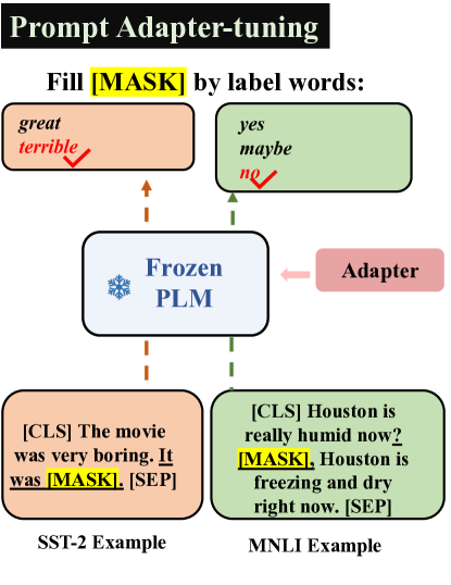
Figure 3: The underlined text depicts task prompt to transform classification into Fill-in-MASK task. Label words are used as proxy for original task labels.

However, this introduces a gap between pre-training and fine-tuning objective with disparate label spaces and additional randomly initiated parameters $W$ introduced for task-specific fine-tuning. This is particularly challenging for few-shot classic fine-tuning, where the limited labeled data is inadequate for adapting the task-specific head and PLM weights effectively. Prompt-based FN (Schick and Schütze, 2021b; Gao et al., 2021) addresses this gap, by re-formulating the objective as a cloze-style auto-complete task. This is done by adding a phrase (also called prompt) to a sentence like $x_{1}=\$“contains no wit, only labored gags" in the form of $\tilde{x}=x_{1}\ \oplus$ “It was [MASK]", where $\oplus$ denotes concatenation of two strings; and output mappings (also called verbalizers) from vocabulary $\mathcal{V}$ to the label space $\mathcal{Y}$ like “{great, terrible}" corresponding to positive and negative classes (refer to Figure 3 for an example). The probability of predicting class $y\in\mathcal{Y}$ is equal to calculating the probability of corresponding label word $v\in\mathcal{V}$:

$$\vspace{-0.1in}p(\mathrm{[MASK]}=v|\tilde{x})=\frac{\exp(W^{T}_{v}\cdot h_{\mathrm{[MASK]}})}{\sum_{v^{\prime}\in V}\exp(W^{T}_{v^{\prime}}\cdot h_{\mathrm{[MASK]}})}$$ (1)

where $W_{v}$ indicates the tunable parameters. Since it is identical to masked language modeling (MLM), $W_{v}$ is initialized by pre-trained weights of PLMs.

In this work, we demonstrate lite self-training with unlabeled data to significantly improve prompt fine-tuning of PLMs in few-shot settings.

3 Related Works

Few-shot and Semi-supervised Learning. Recent works have explored semi-supervised methods for few-shot learning with task-specific unlabeled data, including data augmentation (Xie et al., 2019; Vu et al., 2021), self-training (He et al., 2019; Mukherjee and Awadallah, 2020; Wang et al., 2021c) and contrastive learning (Gunel et al., 2020). GPT-3 (Brown et al., 2020) leverages massive scale with 175 billion parameters to obtain remarkable few-shot performance on several NLU tasks given natural language prompts and a few demonstrations for the task. Recent works (Schick and Schütze, 2021a; Gao et al., 2021) extend this idea of prompting to language models like BERT (Devlin et al., 2019b) and RoBERTa (Liu et al., 2019b). The most related work to ours is iPET (Schick and Schütze, 2021a), which combines prompt-based FN with semi-supervised learning. While iPET ensembles multiple fully-tuned models, we develop a lightweight prompted self-training framework to achieve both data and parameter efficiency.

Few-shot adaptation works (Finn et al., 2017; Li et al., 2019; Zhong et al., 2021; Wang et al., 2021b, a; Beck et al., 2021) train models on massive labeled data on source tasks and develop techniques to adapt them to a target task with few-shot labels. For instance, Beck et al. (2021) first trains on miniImagenet with 38,400 labeled examples (64 classes and 600 samples per class). Similarly,  Zhong et al. (2021); Beck et al. (2021) first train their models on thousands of labels from the source task to study few-shot target adaptation. In contrast, we focus on single-task true few-shot learning with only 10 to 30 labeled examples available overall and no auxiliary supervision labels. Refer to Perez et al. (2021) for an overview of true few-shot learning for NLU. The objective of few-shot adaptation and true few-shot learning is also quite different. The objective of true few-shot learning is to learn a new task with limited labeled data while the objective of few-shot adaptation is to efficiently transfer to a new task/domain with limited labeled data. Thus, few-shot adaptation leverages multi-task setting with auxiliary labeled data from the source tasks that are not available in our setting. The most relevant works to our setup (Gao et al., 2021; Wang et al., 2021c; Schick and Schütze, 2021a; Mukherjee and Awadallah, 2020) are used as baselines in our paper.

Light-weight tuning. Standard fine-tuning methods tune all trainable model parameters for every task. Recent efforts have focused on lightweight tuning of large PLMs by updating a small set of parameters while keeping most of parameters in PLMs frozen, including prefix tuning (Li and Liang, 2021), prompt token tuning (Lester et al., 2021a) and Adapter tuning (Houlsby et al., 2019; Pfeiffer et al., 2020). All of the above works focus on fully supervised settings with thousands of labeled examples using classic fine-tuning. In contrast, we focus on few-shot learning settings leveraging prompts for model tuning, where we make several observations regarding the design and placement of adapters in few-shot settings in contrast to its resource-rich counterpart. Some recent works (Beck et al., 2021; Zhong et al., 2021) pre-train adapters with full supervision with thousands of labeled examples from source tasks for few-shot target adaptation. Different from this, we explore adapter tuning for single-task few-shot learning without any auxiliary supervision labels.

4 Methodology

4.1 Overview

We adopt a PLM (e.g., RoBERTa (Liu et al., 2019b)) as the shared encoder for both the student and teacher for self-training. The shared PLM encoder is frozen and not updated during training. We introduce tunable adapter parameters in both teacher and student (discussed in Section 4.2) that are iteratively tuned during self-training. Refer to Figure 2 for steps in the following discussion.

We first use prompt-based fine-tuning to update the teacher adapter (Step 1) with few-shot labeled examples and leverage the teacher model to assign pseudo-prompt labels (Step 2) on unlabeled data $\mathcal{D}^{u}$. The teacher is often uncertain in few-shot learning and produces noisy pseudo-labels. Therefore, we adopt meta-learning (discussed in Section 4.3) to re-weight the noisy pseudo-labeled samples (Step 3). The re-weighted data is used to train the student adapter (Step 4). Since adapter training with noisy pseudo labels is quite unstable, we introduce knowledge distillation warmup (discussed in Section 4.3.1). Finally, we assign the trained student adapter to be the new teacher adapter (Step 5). Following true few-shot learning settings, we do not use any held-out development or validation set. Therefore, we repeat the above steps for a pre-defined number of times ($M=6$). The overall training procedure is summarized in Algorithm 1 (Appendix B). Throughout the training, we keep the shared student and teacher encoder parameters frozen and update the corresponding adapter parameters along with their language model heads.

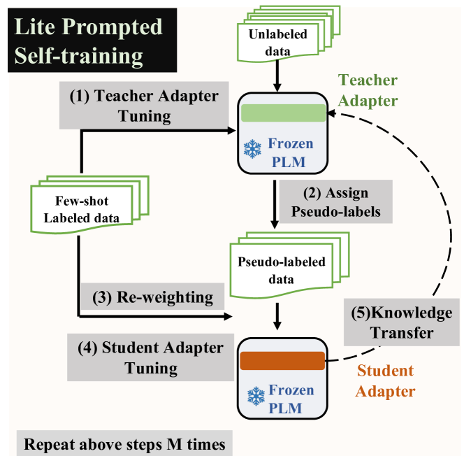
Figure 2: Lite prompted self-training on unlabeled data with prompts and adapters make parameter-efficient few-shot learners with LiST.

4.2 Lightweight Prompt Adapter Tuning

The predominant methodology for task adaptation is to tune all of the trainable parameters of the PLMs for every task. This raises significant resource challenges both during training and deployment. A recent study (Aghajanyan et al., 2021) show that PLMs have a low instrinsic dimension that can match the performance of the full parameter space. To adapt PLMs for downstream tasks with a small number of parameters, adapters (Houlsby et al., 2019) have recently been introduced as an alternative approach for lightweight tuning. Consider the following scenario for demonstration, where we want to use RoBERTa-large with $\mathcal{M}=355M$ parameters as the PLM for $\mathcal{T}=100$ tasks. Full fine-tuning for this scenario requires updating and storing $\mathcal{M}\times\mathcal{T}=35.5B$ parameters. Now, consider fine-tuning with LiST that requires $\mathcal{A}=14M$ (tunable) adapter parameters for every task while keeping the PLM fixed. This results in overall $\mathcal{M}+\mathcal{A}\times\mathcal{T}=1.8B$ parameters, thereby, reducing the overall storage cost by 20x. Adapters have been shown to match the PLM performance in fully supervised settings with thousands of training labels in classic fine-tuning. In contrast, this is the first work to study the role of adapters in few-shot prompt-based FN. We explore different design and placement choices of adapters in few-shot settings and investigate the performance gap with fully supervised as well as fully tunable parameter space.

The adapter tuning strategy judiciously introduces new parameters into the original PLMs. In contrast to standard prompt-based FN that updates all the PLM parameters $\Theta_{\mathrm{PLM}}$, prompt-adapter tuning only updates the newly introduced adapter parameters as well as the (masked) language model head of the PLM (jointly denoted as $\psi$), while keeping the remaining parameters of the original network frozen. The adapter used in LiST consists of two fully connected layers as shown in Figure 4, where a feedforward layer down projects input representations to a low dimensional space $d$ (referred as the bottleneck dimension), and another feedforward layer up projects the low-dimensional features back to the original dimension. However, these newly-inserted parameters can cause divergence resulting in up to $20\%$ performance degradation in few-shot settings (discussed in Section 5.3). To handle this issue, we adopt a skip-connection design where the adapter parameters are initialized with zero-mean small Gaussian noise.

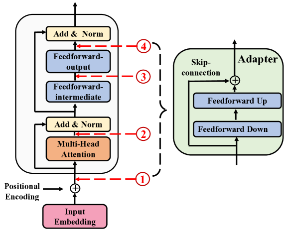
Figure 4: LiST explores several adapter placement choices (numbered positions in left) in standard Transformer architecture, with adapter design shown in right.

Adapter placement. Prior works on lightweight adaptation tune bias (Cai et al., 2020b) or embeddings (Lester et al., 2021a) of Transformers in fully-supervised settings for improving parameter-efficiency with minimal performance loss. However, for few-shot settings, we note that adapter placement is critical to bridge the performance gap with that of a fully tunable model and the choices of tuning bias or embedding can result in upto 10% performance degradation (discussed in Section 5.3). To this end, we explore several choices of adapter placement (refer to Figure 4) corresponding to the most important transformer modules, namely, embedding, intermediate feedforward, output feedforward and attention module in every layer of the Transformer. Based on empirical experiments (refer to Section 5.3) across six diverse NLU tasks, we observe the feedforward output and attention modules to be the most important components for parameter-efficient adaption in few-shot settings.

Formally, consider $\widetilde{\mathcal{D}}^{Train}_{K}=\{\widetilde{x}^{l},\widetilde{y}^{l}\}$ to be the few-shot labeled data and $\widetilde{\mathcal{D}}^{U}=\{\widetilde{x}_{u}\}$ to be the unlabeled data, where we transform the input sequences $x$ to cloze-style input $\widetilde{x}$ containing a single mask following the prompting strategy outlined in Section 2. We use the same pattern templates and verbalizers (output mapping from the task-specific labels $\mathcal{Y}$ to single tokens in the vocabulary $\mathcal{V}$) from traditional prompt-based FN works (Gao et al., 2021). Given the above adapter design and placement of choice with parameters $\psi$, a dataset $\widetilde{\mathcal{D}}_{K}^{Train}$ with shots $K$, a PLM encoder $enc$ with parameters $\Theta_{\mathrm{PLM}}$, where $\Theta_{\mathrm{PLM}}\gg\psi$, we want to perform the following optimization for efficient model adaptation:

$$\psi\leftarrow\operatorname*{arg\,min}_{\psi}\ \mathcal{L}(\widetilde{\mathcal{D}}_{K}^{Train};\Theta_{\mathrm{PLM}},\psi)\vspace{-0.1in}$$ (2)

4.3 Re-weighting Noisy Prompt Labels

Consider $\{\hat{y}^{(t)}_{n}\}_{n=1}^{N}$ to be the pseudo prompt-labels (for the masked tokens in $\widetilde{x}^{u}_{n}\in\widetilde{X}$) from the teacher $(\Theta_{\mathrm{PLM}},\hat{\psi}_{\mathrm{tea}})$ in the $t$-th iteration where $N$ is the number of unlabeled instances and $\hat{\psi}_{\mathrm{tea}}$ represent the teacher adapter parameters. In self-training, the student model is trained to mimic the teacher predictions on the transfer set. Consider $\mathcal{L}(\hat{y}^{(t)}_{n},\mathrm{enc}(\widetilde{x}^{u}_{n};\Theta_{\mathrm{PLM}},\psi^{(t)}_{\mathrm{stu}}))$ to be the loss of the student model with parameters $(\Theta_{\mathrm{PLM}},\psi^{(t)}_{\mathrm{stu}})$ on the pseudo-labeled data in the $t$-th iteration, where $\Theta_{\mathrm{PLM}}$ and $\psi_{\mathrm{stu}}$ represent the PLM and the student adapter parameters respectively. In order to reduce error propagation from noisy pseudo-labels, we leverage meta-learning to re-weight them based on the student model loss on the validation set as our meta-objective. The intuition of meta re-weighting is to measure the impact or weight of a pseudo-labeled example given by its performance on the validation set. Since we do not have access to a separate validation set in the spirit of true few-shot learning, we leverage the labeled training set $\widetilde{\mathcal{D}}^{Train}_{K}$ judiciously for re-weighting. To this end, we leverage the idea of weight perturbation (Ren et al., 2018) to set the weight of pseudo-labeled example $(\widetilde{x}^{u}_{i},\hat{y}^{(t)}_{i})$ to $\epsilon^{(t)}_{i}$ at iteration $t$ as:

$$\mathcal{L}^{(t)}_{r}(\epsilon,\psi)=\frac{\sum_{i=1}^{N}[\epsilon^{(t)}_{i}\cdot\mathcal{L}(\hat{y}^{(t)}_{i},\mathrm{enc}(\widetilde{x}^{u}_{i};\Theta_{\mathrm{PLM}},\hat{\psi}^{(t-1)}_{\mathrm{stu}}))]}{N}.\vspace{-0.5em}$$ (3)

$$\hat{\psi}^{(t)}_{\mathrm{stu}}(\epsilon)=\hat{\psi}^{(t-1)}_{\mathrm{stu}}-\alpha\triangledown\mathcal{L}^{(t)}_{r}(\epsilon,\psi).\vspace{-0.5em}$$ (4)

where $\alpha$ is the step size. Weight perturbation is used to discover data points that are most important to improve performance on the validation set. Optimal value for the perturbation $\epsilon^{(t)*}_{i}$ can be obtained via minimizing student model loss on the validation set at iteration $t$ as:

$$\epsilon^{(t)*}_{i}=\operatorname*{arg\,min}_{\epsilon_{i}}\frac{\sum_{i=1}^{|\widetilde{\mathcal{D}}^{Train}_{K}|}\mathcal{L}({y}_{i},\mathrm{enc}(x_{i};\Theta_{\mathrm{PLM}},\hat{\psi}^{(t)}_{stu}(\epsilon_{i}))}{|\widetilde{\mathcal{D}}^{Train}_{K}|}$$ (5)

To obtain a cheap estimate of the meta-weight at step $t$, we take a single gradient descent step on a mini-batch $\widetilde{\mathcal{D}}^{(t)}\in\widetilde{\mathcal{D}}^{Train}_{K}$ as:

$$u_{i}^{(t)}=-\frac{\partial}{\partial{\epsilon_{i}}}\bigg{(}\frac{\sum_{i=1}^{|\widetilde{\mathcal{D}}^{(t)}|}\mathcal{L}(y_{i},\mathrm{enc}(\widetilde{x}_{i};\Theta_{\mathrm{PLM}},\hat{\psi}^{(t)}_{stu}(\epsilon)))}{{|\widetilde{\mathcal{D}}^{(t)}|}}\bigg{)}$$ (6)

The weight $w_{i}^{(t)}$ of $(\widetilde{x}^{u}_{i},\hat{y}^{(t)}_{i})$ at iteration $t$ is set to be proportional to the negative gradient $u_{i}^{(t)}$ to reflect the importance of pseudo-labeled samples. Samples with negative weights are filtered out since they could potentially degrade the student performance. Finally, we update student adapter parameters $\psi_{\mathrm{stu}}$ while accounting for re-weighting as:

$$\mathcal{L}^{(t)}=\frac{1}{N}\sum_{i=1}^{N}[w_{i}^{(t)}\cdot\mathcal{L}(\hat{y}^{(t)}_{i},\mathrm{enc}(\widetilde{x}^{u}_{i};\Theta_{\mathrm{PLM}},\hat{\psi}^{(t-1)}_{\mathrm{stu}}))]\big{)}.$$ (7)

4.3.1 Knowledge Distillation For Student Warmup

Meta re-weighting leverages gradient as a proxy to estimate the weight of noisy pseudo labels. However, the gradients of adapter parameters $\psi$ are not stable in the early stages of training due to random initialization and noises in pseudo labels. This instability issue is further exacerbated with adapter tuning that usually requires a larger learning rate (Pfeiffer et al., 2020). Therefore, to stabilize adapter tuning, we propose a warmup training stage via knowledge distillation (Hinton et al., 2015) to first tune adapter parameters via knowledge distillation loss for $T_{warm}$ steps and then we continue self-training with re-weighted updates via Eq. 7. Since the re-weighting procedure has access to our training labels, we do not use labeled data in knowledge distillation while using only the unsupervised consistency loss between teacher model $(\Theta_{\mathrm{PLM}},\hat{\psi}_{\mathrm{tea}})$ and student model $(\Theta_{\mathrm{PLM}},\hat{\psi}_{\mathrm{stu}})$ on unlabeled data as.

$$\operatorname*{arg\,min}_{\hat{\psi}_{stu}}\mathrm{KL}(f(\widetilde{x}^{u};\Theta_{\mathrm{PLM}},\hat{\psi}_{\mathrm{tea}})\;\|\;f(\widetilde{x}^{u};\Theta_{\mathrm{PLM}},\hat{\psi}_{\mathrm{stu}})).$$ (8)

We further validate the effectiveness of knowledge distillation for warmup with ablation analysis.

4.3.2 Student Adapter Re-initialization

A typical challenge in few-shot settings is the lack of a separate validation set. In the spirit of true few-shot learning, we use only the available few-shot labeled examples $\widetilde{\mathcal{D}}^{Train}_{K}$ as the validation set for meta-learning of the student model. This poses an interesting challenge of preventing label leakage. To address this issue, we re-initialize the student adapter parameters every time at the start of each self-training iteration to mitigate interference with labeled data. Note that the student and teacher model share the encoder parameters $\Theta_{\mathrm{PLM}}$ that are always kept frozen and not updated during training.

5 Experiments

5.1 Experimental Setup

Dataset. We perform large-scale experiments with six natural language understanding tasks as summarized in Table 6. We use four tasks from GLUE (Wang et al., 2019), including MNLI (Williams et al., 2018b) for natural language inference, RTE (Dagan et al., 2005; Bar Haim et al., 2006; Giampiccolo et al., 2007; Bentivogli et al., 2009) for textual entailment, QQP for semantic equivalence and SST-2 (Socher et al., ) for sentiment classification. The results are reported on their development set following (Zhang et al., 2021). MPQA (Wiebe et al., 2005) and Subj (Pang and Lee, 2004) are used for polarity and subjectivity detection, where we follow Gao et al. (2021) to keep $2,000$ examples for testing and use remaining examples for semi-supervised learning.

For each dataset, we randomly sample $|\mathcal{K}|\in\{10,20,30\}$ manually labeled samples from the training data, and add the remaining to the unlabeled set while ignoring their labels – following standard setups for semi-supervised learning. We repeatedly sample $K$ labeled instances five times, run each model with $5$ different seeds and report average performance with standard deviation across the runs. For the average accuracy over 6 tasks, we did not include standard deviation across tasks. Furthermore, for every split and shot, we sample the labeled data such that $\mathcal{D}_{10}^{Train}\subset\mathcal{D}_{20}^{Train}\subset\mathcal{D}_{30}^{Train}$ to evaluate the impact of incremental sample injection.

Following true few-shot learning setting (Perez et al., 2021), we do not use additional development set beyond $|\mathcal{K}|$ labeled samples for any hyper-parameter tuning or early stopping. The performance of each model is reported after fixed training epochs (see Appendix for details).

Labels	Models	Avg	#Tunable	MNLI (m/mm)	RTE	QQP	SST-2	Subj	MPQA
			Params	(acc)	(acc)	(acc)	(acc)	(acc)	(acc)
$|\mathcal{K}|=30$	Classic FN	60.9	355M	38.0 (1.7) / 39.0 (3.1)	51.4 (3.7)	64.3 (8.1)	65.0 (11.5)	90.2 (2.2)	56.1 (5.3)
	Prompt FN	77.6	355M	62.8 (2.6) / 64.1 (3.3)	66.1 (2.2)	71.1 (1.5)	91.5 (1.0)	91.0 (0.5)	82.7 (3.8)
$|\mathcal{K}|=30$ +Unlabeled Data	UST	65.8	355M	40.5 (3.3) / 41.5 (2.9)	53.4 (1.7)	61.8 (4.3)	76.2 (11.4)	91.5 (2.1)	70.9 (6.2)
	MetaST	62.6	355M	39.4 (3.9) / 40.5 (4.4)	52.9 (2.0)	65.7 (6.2)	65.3 (15.2)	91.4 (2.3)	60.5 (3.6)
	iPET	75.5	355M	61.0 (5.8) / 61.8 (4.7)	54.7 (2.8)	67.3 (4.1)	93.8 (0.6)	92.6 (1.5)	83.1 (4.8)
	PromptST	77.2	14M	61.8 (1.9) / 63.1 (2.9)	66.2 (5.1)	71.4 (2.1)	91.1 (1.4)	90.3 (1.5)	81.8 (2.5)
	LiST	82.0	14M	73.5 (2.8) / 75.0 (3.7)	71.0 (2.4)	75.2 (0.9)	92.8 (0.9)	93.5 (2.2)	85.2 (2.1)
Supervision with	Classic FN	90.9	355M	89.6 / 89.5	83.0	91.8	95.2	97.2	88.8
# Full Train	Prompt FN	92.0	355M	89.3 / 88.8	88.4	92.1	95.9	97.1	89.3

Table 1: Performance comparison of different tuning strategies on different NLU tasks with RoBERTa-large as the encoder with standard deviation in parantheses. UST, MetaST, PromptST and iPET are semi-supervised methods using unlabeled data, whereas Classic and Prompt FN only use labeled data.

Baselines. In addition to classic-tuning (Classic FN), we adopt prompt-based fine-tuning (Prompt FN) from Gao et al. (2021) as labeled-only baselines. We also adopt several state-of-the-art semi-supervised baselines including UST (Mukherjee and Awadallah, 2020), MetaST (Wang et al., 2021c) and iPET (Schick and Schütze, 2021a). UST and MetaST are two self-training methods which are based on classic fine-tuning strategies. iPET is a semi-supervised method leveraging prompt-based fine-tuning and prompt ensembles to obtain state-of-the-art performance. While iPET ensembles multiple fully-tuned models, we develop a lite self-training framework to achieve both data and parameter efficiency. As the strongest semi-supervised baseline, we implement a new method PromptST based on self-training using prompts and adapters (as a subset of the methods used in LiST), but without any re-weighting, or KD warmup that are additionally used in LiST. The methods Prompt FN, PromptST and LiST adopt same prompts and label words as in Gao et al. (2021). We implement our framework in Pytorch and use Tesla V100 gpus for experiments. Prompts used in experiments and hyper-parameter configurations are presented in Appendix.

5.2 Key Results

Table 1 shows the performance comparison among different models with $|\mathcal{K}|=30$ labeled examples with fixing RoBERTa-large as the encoder. Fully-supervised RoBERTa-large trained on thousands of labeled examples provides the ceiling performance for the few-shot setting. We observe LiST to significantly outperform other state-of-the-art baselines along with $96\%$ reduction in tunable parameters, achieving both labeled data- and parameter-efficiency. More specifically, LiST improves over Classic FN, Prompt FN, iPET and PromptST by $34.6\%$, $5.7\%$, $8.6\%$ and $6.2\%$ respectively in terms of average performance on six tasks. This demonstrates the impact of self-training with unlabeled data and prompt-based FN. Additionally, iPET and LiST both leverage prompt-based FN to significantly improve over UST and MetaST that use classic fine-tuning strategies, confirming the effectiveness of prompt-based FN in the low data regime. iPET ensembles multiple prompts with diverse qualities and under-performs Prompt FN on average in our few-shot setting without using any development set.

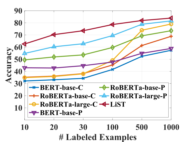
(a) MNLI

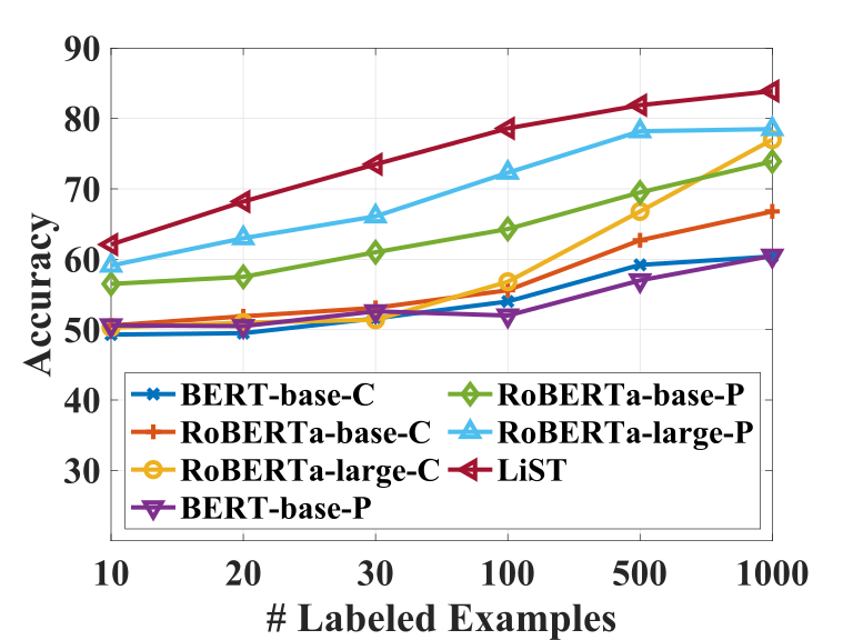
(b) RTE

Figure 5: Performance comparison of Classic-tuning (denoted as “C") and prompt-based fine-tuning (denoted as “P") with LiST on MNLI and RTE using language model encoders of different sizes.

Labels	Fine-tuning Method	Avg	MNLI (m/mm)	RTE	QQP	SST-2	Subj	MPQA
			(acc)	(acc)	(acc)	(acc)	(acc)	(acc)
$|\mathcal{K}|=10$	GPT-3 In-context	61.5	36.4 (0.8) / 36.7 (1.3)	53.2 (1.8)	61.8 (3.0)	86.6 (7.4)	61.0 (11.2)	66.7 (9.5)
	Prompt-based FN	69.3	54.8 (3.7) / 55.6 (4.6)	60.0 (4.4)	58.7 (4.6)	89.5 (1.7)	84.5 (8.6)	67.8 (6.9)
	LiST	72.8	62.6 (6.6) / 63.3 (7.7)	61.2 (4.9)	60.4 (7.0)	91.1 (1.2)	91.0 (1.6)	70.3 (10.6)
$|\mathcal{K}|=20$	GPT-3 In-context	57.4	38.0 (2.0) / 38.4 (2.8)	54.5 (1.5)	64.2 (1.6)	79.1 (2.3)	51.2 (1.7)	72.4 (8.5)
	Prompt-based FN	75.4	60.3 (2.0) / 61.6 (2.7)	64.3 (2.4)	67.8 (4.2)	90.6 (1.8)	88.3 (2.2)	80.6 (7.5)
	LiST	79.5	68.9 (3.1) / 70.4 (3.3)	69.0 (3.5)	72.3 (3.7)	92.3 (1.2)	91.5 (1.3)	82.2 (5.1)
$|\mathcal{K}|=30$	GPT-3 In-context	61.5	37.9 (2.2) / 38.5 (2.9)	53.4 (2.2)	65.0 (1.7)	79.7 (7.1)	57.7 (6.4)	74.8 (6.9)
	Prompt-based FN	77.6	62.8 (2.6) / 64.1 (3.3)	66.1 (2.2)	71.1 (1.5)	91.5 (1.0)	91.0 (0.5)	82.7 (3.8)
	LiST	82.0	73.5 (2.8) / 75.0 (3.7)	71.0 (2.4)	75.2 (0.9)	92.8 (0.9)	93.5 (2.2)	85.2 (2.1)

Table 2: Average performance and standard deviation of GPT-3 ($175B$ params) in-context learning, Prompt-based FN and LiST methods using Roberta-Large ($355M$ params) encoder with varying number of training labels $|\mathcal{K}|$. LiST updates $14M$ params in contrast to Prompt-based FN with full model tuning.

Figure 5 compares the performance of tuning methods with varying number of training labels and encoders of different sizes. We observe that large models are more data-efficient compared to smaller models. However, large fully-tunable models are expensive to use in practise. We observe that LiST with small number of tunable parameters consistently outperforms fully-tunable classic and prompt-based FN strategies in all labeled data settings, demonstrating both data and parameter efficiency. Additional results with different backbone encoders and varying number of shots and fine-tuning strategies are presented in the Appendix in Tables 13,  14,  15 and 19 that demonstrate similar trends as we observe in Table 1 and Figure 5.

Comparison with GPT-3 in-context Learning. We perform a comparison between GPT-3 in-context learning, RoBERTa-large Prompt-based fine-tuning and LiST methods with varying number of training labels in Table 2. For a fair comparison, the prompt and label words are same for the three approaches. We observe that LiST outperforms GPT-3 In-context learning and Prompt-based FN consistently with different number of labels.

5.3 Adapter Analysis

In this section, we explore adapter design choices for prompt-based FN with RoBERTa-large as encoder using only few-shot labeled data.

Tuning	#Params	Avg	Diff
Full	355M	77.6	—
2-5 Embedding	53M	67.0	-10.7
Attention	101M	77.0	-0.6
FF-output	102M	77.6	+0.0
FF-intermediate	102M	75.9	-1.7

Table 3: Average accuracy on tuning different modules of RoBERTa-large with $|\mathcal{K}|=30$ labels on six tasks. Diff shows performance change relative to Full tuning.

Where to insert an adapter in Transformers? In order to answer this question, we conduct an experiment to study the role of various Transformer modules in few-shot prompt-based FN. To this end, we tune a given module along with the language model head while keeping all other parameters frozen. Table 3 shows the performance comparison of tuning specific modules on six tasks with varying number of labeled examples. The main modules of RoBERTa include Embedding, Attention, Feedforward Output and Feedforward Intermediate layers. We observe that tuning only the Feedforward Output or the Attention module delivers the best performance across most tasks with few-shot labels. Correspondingly, this motivated us to insert our adapter parameters into these two modules. More detailed results are presented in Appendix Table 11.

Tuning	#Params	Avg
Head-only	1M	66.9
Bias-only (Cai et al., 2020b)	1M	68.3
Prompt-tuning (Lester et al., 2021b)	1M	56.4
LiST Adapter (2)	1M	72.7
Houlsby Adapter (Houlsby et al., 2019)	14M	57.9
LiST Adapter (128)	14M	77.7
Full tuning	355M	77.6

Table 4: Average accuracy of several lightweight parameter-efficient tuning strategies with $|\mathcal{K}|=30$ labels without unlabeled data on six tasks along with the number ($\#$) of tunable parameters. Each task is run with 5 different seeds. LiST Adapter performance with different bottleneck dimension $d$ of its adapters is shown in parantheses.

Comparison with other lightweight parameter efficient model tuning strategies. To validate the effectiveness of LiST adapters, we compare it against several baselines in Table 4. For a fair comparison, we present two variations of our LiST adapters with bottleneck dimensions $d$= $\{2,128\}$ corresponding to $1M$ and $14M$ parameters to match other adapter capacities; all the approaches in Table 4 are trained with 30 labels only without unlabeled data for a fair comparison. (1) Bias-only is a simple but effective lightweight method, which tunes bias terms of PLMs while keeping other parameters frozen. (2) Tuning head layers is widely used as a strong baseline for lightweight studies (Houlsby et al., 2019), where we tune last two layers including language model head while freezing other parameters. (3) prompt-tuning is a lightweight method which only updates task prompt embedding while keeping entire model frozen. (4) Houlsby Adapter tunes inserted adapter parameters keeping the encoder frozen by adopting classic tuning strategy. Besides these lightweight methods, we also present a performance comparison with full model tuning as a strong baseline. More detailed results are presented in Appendix in Tables 12 and  20 that demonstrate similar trends.

Table 4 shows that LiST is able to match the performance of full model prompt-based FN with bottleneck dimension $d=128$ and outperforms all other baselines with similar capacities. While lightweight model tuning choices like tuning the bias or inserting adapters into classic tuning models are shown to be effective in fully-supervised settings (Cai et al., 2020b; Houlsby et al., 2019), we observe them to under-perform for few-shot learning. We observe that simpler tuning choices like Head-only and Bias-only results in upto $10\%$ performance degradation. Houlsby adapter and Prompt-only results in upto $20\%$ performance degradation. In constrast, LiST adapter is able to match the performance of full tuning in few-shot setting, demonstrating the importance of adapter placement choices and parameter initialization.

5.4 Ablation Analysis

Table 5 demonstrates the impact of different components and design choices of LiST.

$\bullet$ Adapter training stability. Training with very few labels and noisy pseudo labeled data results in instability for adapter tuning. To demonstrate training stability, we include the average accuracy and standard deviation across several runs and splits as metrics. We observe that hard pseudo-labels hurt the model performance compared to soft pseudo-labels and exacerbate the instability issue. This is in contrast to observations from classic fine-tuning (Wang et al., 2021c). A potential reason could be that the well pre-trained language model head for prompt-based FN is able to capture better associations among different prompt labels.

Method	Avg Acc	Avg Std	Datasets
			MNLI (m/mm)	RTE
LiST ($14M$)	72.6	2.8	73.5 (2.8) / 75.0 (3.7)	71.0 (2.4)
w/o re-init	68.3	4.2	66.7 (2.8) / 68.3 (4.3)	69.0 (4.9)
w/o KD Warmup	68.8	8.8	67.9 (12.9) / 69.0 (13.1)	69.2 (4.5)
w/o Re-weighting	71.6	4.0	72.9 (3.4) / 74.2 (4.5)	69.7 (4.1)
w/ Hard Pseudo-Labels	70.9	4.4	71.7 (3.8) / 73.0 (5.4)	69.5 (4.2)
LiST w/o Adapter ($355M$)	72.6	2.5	73.6 (2.7) / 74.8 (2.7)	71.2 (2.3)

Table 5: Ablation analysis of LiST with 30 labels on MNLI and RTE with tunable parameters in parantheses.

$\bullet$ Knowledge Distillation Warmup. In this ablation study, we remove the warmup phase with knowledge distillation from LiST (denoted as “LiST w/o KD Warmup”). Removing this component results in $4\%$ performance drop in terms of average accuracy and $300\%$ larger standard deviation – demonstrating the importance of KD Warmup in stabilizing LiST training.

$\bullet$ LiST versus LiST w/o Adapter. In LiST, we only fine-tune the adapter and language model head while keeping other encoder parameters frozen to achieve parameter efficiency. Table 5 shows that LiST using only $4\%$ tunable parameters is able to match the performance of fully tunable LiST (that is without using any adapters and tuning all encoder parameters) on MNLI and RTE – demonstrating the effectiveness of our lightweight design. More ablation results with varying shots are presented in Appendix in Tables 16, 17 and 18 that demonstrate similar trends as in Table 5.

6 Conclusions and Future Work

We develop a new method LiST for lightweight tuning of large language models in few-shot settings. LiST uses prompted self-training to learn from large amounts of unlabeled data from target domains. In order to reduce the storage and training cost, LiST tunes only a small number of adapter parameters with few-shot labels while keeping the large encoder frozen. With only $30$ labels for every task, LiST improves by upto $35\%$ over classic fine-tuning and $6\%$ over prompt-tuning while reducing $96\%$ of the tunable parameters. With significant reduction in the cost of (data) annotation and overall model footprint, LiST provides an efficient framework towards life-long learning of AI agents (Biesialska et al., 2020). While adapters reduce storage cost, LiST does not reduce inference latency given the PLM backbone. A future work is to consider combining model compression techniques (Han et al., 2015; Cai et al., 2020a) with adapters to reduce FLOPS and latency.

7 Ethical Considerations

In this work, we introduce a lightweight framework for self-training of language models with only a few labeled examples. We expect that progress and findings presented in this paper could further benefit NLP applications with limited labeled data. In the real-world setting, it is usually not only expensive to obtain large-scale labeled data for each task but also brings privacy and compliance concerns when large-scale data labeling is needed. The privacy concerns could be further exacerbated when dealing with sensitive user data for peronslization tasks. Our framework which only needs few-shot labeled data could help in this to obtain state-of-the-art-performance while alleviating privacy concerns. The proposed framework is tested across different tasks and could be used for applications in various areas including finance, legal, healthcare, retail and other domains where adoption of deep neural network may have been hindered due to lack of large-scale manual annotations on sensitive user data.

While our framework advance the progress of NLP, it also suffers from associated societal implications of automation ranging from job losses for workers who provide annotations as a service as well as for other industries relying on human labor. Moreover, it may bring additional concerns when NLP models are used by malicious agents for propagating bias, misinformation and indulging in other nefarious activities. However, many of these concerns can also be alleviated with our framework to develop better detection models and mitigation strategies with only a few representative examples of such intents.

The proposed method is somewhat compute-intensive as it involves large-scale language model. This might impose negative impact on carbon footprint from training the described models. In order to reduce the storage and training cost, the proposed design tunes only a small number of adapter parameters with few-shot labels while keeping the large encoder frozen.

Appendix A Datasets

A.1 Dataset information

Table 6 summarize dataset statistics and task descriptions. All the datasets are in English Language. The licence information is as follows.

MNLI: The majority of the corpus is released under the OANC’s license, which allows all content to be freely used, modified, and shared under permissive terms. The data in the FICTION section falls under several permissive licenses; Seven Swords is available under a Creative Commons Share-Alike 3.0 Unported License, and with the explicit permission of the author, Living History and Password Incorrect are available under Creative Commons Attribution 3.0 Unported Licenses; the remaining works of fiction are in the public domain in the United States (but may be licensed differently elsewhere).

RTE: The dataset is public release but the corresponding licence information is not found in the source website .

QQP: We did not find the responding license. The source website  is not accessible.

SST-2 dataset: CC0: Public Domain

Subj: The dataset is public release but the Licence information is not presented in the source website .

MPQA: The dataset is public release. Made available under the terms of GNU General Public License. They are distributed without any warranty.

We follow the licence of datasets for research use. We manually check no offensive content in our few-shot training dataset.

Category	Dataset	#Labels	#Full Train	#Test	Type	Labels
sentence- pair	MNLI	3	392,702	9,815	NLI	entailment, neutral, contradiction
	RTE	2	2,490	277	NLI	entailment, not_entailment
	QQP	2	363,846	40,431	paraphrase	equivalent, not_equivalent
single- sentence	SST-2	2	6,920	872	sentiment	positive, negative
	Subj	2	8,000	2,000	subjectivity	subjective, objective
	MPQA	2	8,606	2,000	opinion polarity	positive, negative

Table 6: Dataset summary and task descriptions. For each task, we sample $\mathcal{K}\in\{10,20,30\}$ labeled examples to form five different splits with different random seeds from the original training set, and add the remaining to the unlabeled set while ignoring their labels.

A.2 Prompts

Table  7 summarizes manually-designed prompts and label words for each dataset in our experiments. These prompts and label words were adopted from (Gao et al., 2021).

Task	Prompt	Label words
SST-2	<$S_{1}$> It was [MASK] .	positive: great, negative: terrible
MR	<$S_{1}$> It was [MASK] .	positive: great, negative: terrible
Subj	<$S_{1}$> This is [MASK] .	subjective: subjective, objective: objective
MNLI	<$S_{1}$> ? [MASK] , <$S_{2}$>	entailment: Yes, netural: Maybe, contradiction: No
RTE	<$S_{1}$> ? [MASK] , <$S_{2}$>	entailment: Yes, not_entailment: No
QQP	<$S_{1}$> [MASK] , <$S_{2}$>	equivalent: Yes, not_equivalent: No

Table 7: Task prompt and label words summary. <$S_{1}$> and <$S_{2}$> indicate input sentences.

Appendix B Algorithm Flow

Algorithm 1 summarizes overall flow of LiST. We adopt a light self-training mechanism which keeps the shared student and teacher encoder parameters frozen and only updates the adapter parameters along with the corresponding language model heads. Beside the lightweight tuning design, another key step in our self-training framework is to utilize the few-shot labeled data to fine-tune the student model $\psi^{(T)}_{\mathrm{stu}}$) in every self-training session. Such a step is different with conventional self-training framework, which either leverages labeled data for initial teacher fine-tuning or combine labeled data with unlabeled data for joint training of student model. The iterative usage of unlabeled data and labeled data helps in better teacher initialization before next round of adapter prompt-tuning on $\widetilde{\mathcal{D}}^{Train}_{K}$ which further helps in improving model tuning and the quality of pseudo labels.

Input: Labeled samples $\widetilde{\mathcal{D}}^{Train}_{K}=\{\widetilde{x}^{l},\widetilde{y}^{l}\}$; Unlabeled samples $\widetilde{\mathcal{D}}^{U}=\{\widetilde{x}_{u}\}$; a pre-trained language model with parameters $\Theta_{\mathrm{PLM}}$; randomly initialized Adapter with parameters $\psi$; Number of student training iterations $T$, KD warmup steps $T_{warm}$ and self-training sessions $M$.

Initialize teacher adapter $\psi_{\mathrm{tea}}=\psi^{(0)}$

Tune teacher adapter $\psi_{\mathrm{tea}}$ on small labeled data $\widetilde{\mathcal{D}}^{Train}_{K}$;

for $m\leftarrow 1$ to $M$ do

      

      Initialize the student adapter $\psi_{\mathrm{stu}}=\psi^{(0)}$ ;

      for $t\leftarrow 1$ to $T$ do

             Infer pseudo prompt labels $\{\hat{y}^{(t)}_{n}\}_{n=1}^{N}$ for unlabeled data $\widetilde{\mathcal{D}}^{U}=\{\widetilde{x}_{u}\}$ with teacher model $(\Theta_{\mathrm{PLM}},\psi_{\mathrm{tea}})$;

            Randomly sample a batch of pseudo-labeled samples from $(\widetilde{x}_{u},\hat{y}^{(t)})$;

            if t $<$ T_warm then

                   Train student adapter $\psi_{\mathrm{stu}}$ according to Eq. 8

            else

                  

                  Sample a mini-batch from $\widetilde{\mathcal{D}}^{(t)}\in\widetilde{\mathcal{D}}^{Train}_{K}$ as validation mini-batc for re-weighting;

                  Train student adapter $\psi_{\mathrm{stu}}$ on re-weighted pseudo-labeled samples according to Eq. 7;

             end if

            

       end for

      

      Tune student adapter $\psi^{(T)}_{\mathrm{stu}}$ on small labeled data $\widetilde{\mathcal{D}}^{Train}_{K}$;

      Update the teacher adapter: $\psi_{\mathrm{tea}}=\psi_{\mathrm{stu}}^{(T)}$

end for

Algorithm 1 LiST Algorithm.

Appendix C Experimental Details

C.1 Hyper-parameters

Following the true few-shot learning spirit, we do not have any additional development set for hyper-parameter tuning. Instead we keep all the hyper-parameter same for different tasks, different model families and sizes as well as different shots $K$. We retain most of the default hyper-parameter configurations from related work. For each task, we run the model five times with different data splits and different random seeds in $\{1,2,3,4,5\}$. Our experiments are conducted in few-shot supervision setting and few-shot semi-supervised setting. In the following, we introduce the hyper-parameters for each setting respectively.

Few-shot supervision setting. We set learning rate as 5e-6, training epochs as $400$ and batch size as $4$. The bottleneck dimension $d$ of Adapter is set to $128$. The optimizer is AdamW (Loshchilov and Hutter, 2017) with default settings besides learning rate. We use variance for adapter as 0.002 and observe that the performance is not sensitive to variance values when the scale of variance values are equal or less than 0.002. Since experiments are run with different number of labeled examples, the GPU hours range from 5 minutes to 1 hour per task.

Few-shot semi-supervised setting. For initial teacher fine-tuning, we adopt the same hyper-parameter configuration as in few-shot supervision setting. To facilitate training on a large amounts of unlabeled data, the learning rate in self-training is set to 1e-4 following fully supervised adapter work (Pfeiffer et al., 2020). The batch size of unlabeled data for student adapter training is $16$ and the size of minibatch $\widetilde{\mathcal{D}}\in\widetilde{\mathcal{D}}^{Train}_{K}$ for meta re-weighiting in Eq. 6 is $4$. For each self-training session, we train student adapter for $T=1000$ steps and further fine-tune $50$ epochs on given labeled data. The student KD warmup ratio is set to $60\%$, i.e., $T_{warm}=600$ steps, without extra hyper-parameter tuning. We repeat all the steps in self-training training $M=6$ times. Since experiments are run with different number of labeled examples and datasets, the GPU hours of all approaches are different, ranging from 1 hour to 10 hours per task.

Models	#Params	Avg Acc
BERT-base	110M	67.4
BERT-large	336M	68.0
RoBERTa-base	125M	73.7
RoBERTa-large	355M	77.6
T5-small	60M	66.5
T5-base	220M	71.9
T5-large	770M	77.3

Table 8: Average accuracy of prompt FN with different encoders using $|\mathcal{K}|=30$ labels on six tasks.

C.2 Few-shot Supervision with Varying Model Sizes and Labels

To better understand the role of different model families in few-shot prompt-based FN, we evaluate the performance of representative state-of-the-art PLMs like BERT (Devlin et al., 2019b), RoBERTa (Liu et al., 2019b) and T5 (Raffel et al., 2020) of different sizes (parameters) using varying amounts of labeled data. We report macro-averaged results over six tasks where each has five different splits for easy comparison.

Effect of model choices. Table 8 shows the performance comparison of three representative PLMs with different parameters using prompt-based FN on $30$ labeled samples. We observe that average performance increases with increase in model size within each model family. Overall, we observe RoBERTa models to perform much better than BERT, and marginally outperform T5 models of much bigger size. Accordingly, we use RoBERTa-large as the base encoder for both LiST and other baseline methods.

Effect of varying the number of labels $|\mathcal{K}|$. From Figure  5, we observe prompt-based FN to consistently outperform classic-tuning under all labeled data settings when using the same encoder. With increase in the amount of labeled examples, prompt-based FN and classic-tuning both improve in performance, although with reduced performance gap. This demonstrates prompt-based FN to be the most impactful for low-resource settings with few training labels. LiST improves over both classic and prompt-based FN in all settings with massive reduction in number of tunable parameters.

C.3 Experimental result details

Fine-tuning strategies with varying number of shots. Table 9 shows the performance comparison of RoBERTa-large with two fine-tuning strategies and varying number of labeled samples including zero-shot supervision, few-shot supervision from 10 to 30 and full supervision. Prompt fine-tuning shows competitive performance in zero-shot learning, outperforming classic fine-tuning strategy with 30 labeled examples on several tasks like MNLI and SST-2. As the size of labeled examples increases, the average performance of classic and prompt fine-tuning strategy improves significantly and prompt fine-tuning strategy consistently improves classic fine-tuning with a big gap in the few-shot setting. With full supervision, Prompt fine-tuning strategy and classic fine-tuning strategy achieve similar performance, demonstrating that Prompt fine-tuning is most impactful for low-resource settings with few training labels.

Labels	Models	Avg	MNLI (m/mm)	RTE	QQP	SST-2	Subj	MPQA
			(acc)	(acc)	(acc)	(acc)	(acc)	(acc)
$|\mathcal{K}|=0$	Classic	-	-	-	-	-	-	-
	Prompt	58.4	51.7/52.4	51.3	38.6	83.6	51.4	67.6
$|\mathcal{K}|=10$	Classic	50.0	34.9 (0.3) / 35.2 (0.7)	50.3 (2.1)	61.1 (3.5)	51.8 (2.9)	71.2 (17.5)	52.4 (3.2)
	Prompt	69.3	54.8 (3.7) / 55.6 (4.6)	60.0 (4.4)	58.7 (4.6)	89.5 (1.7)	84.5 (8.6)	67.8 (6.9)
$|\mathcal{K}|=20$	Classic	55.2	35.8 (1.0) / 36.8 (1.5)	51.0 (4.8)	61.3 (9.0)	57.2 (7.7)	84.8 (9.0)	55.9 (4.1)
	Prompt	75.4	60.3 (2.0) / 61.6 (2.7)	64.3 (2.4)	67.8 (4.2)	90.6 (1.8)	88.3 (2.2)	80.6 (7.5)
$|\mathcal{K}|=30$	Classic	59.7	38.0 (1.7) / 39.0 (3.1)	51.4 (3.7)	64.3 (8.1)	65.0 (11.5)	90.2 (2.2)	56.1 (5.3)
	Prompt	77.6	62.8 (2.6) / 64.1 (3.3)	66.1 (2.2)	71.1 (1.5)	91.5 (1.0)	91.0 (0.5)	82.7 (3.8)
Full supervision	Classic	90.7	89.6 / 89.5	83.0	91.8	95.2	97.2	88.8
	Prompt	91.8	89.3 / 88.8	88.4	92.1	95.9	97.1	89.3

Table 9: Average performance and standard deviation of RoBERTa-large with Classic and Prompt-tuning strategies with varying training labels $|\mathcal{K}|$.

Task performance of varying number of shots and models. We show performance changes regarding varying number of shots and varying model choices in Figure 5 and include more detailed results including average accuracy over 5 runs and corresponding standard deviation on MNLI and RTE in Table 10.

Task performance of different modules with varying number of shots. We show the average accuracy on tuning different modules of RoBERTa-large with $|K|=30$ on six tasks in Table 3. In Table 11, we show average accuracy with standard deviation of RoBERTa-large on each task using varying shots of labeled data. We can observe that Feedforward-output performs best in average while Attention module achieves best performance on some tasks. The conclusion is consistent across different shots of labeled data. Such observations motivate us to insert Adapter into Feedforward Output and Attention modules to handle diverse tasks.

Task performance of lightweight model tuning strategies. We show the average accuracy of serveral lightweight strategies with $|K|=30$ labeled examples on six tasks in Table 4. In Table 12, we show average accuracy with standard deviation of lightweight tuning strategies on each task with $|K|=30$ labeled examples. We can observe that LiST Adapter outperforms all the lightweight tuning strategies for all six tasks, demonstrating the effective design in adapter placement and parameter initialization.

Labels	Models	MNLI (m/mm)	RTE
		(acc)	(acc)
$|\mathcal{K}|=10$	BERT-base-Classic	32.1 (1.2) / 32.4 (1.2)	49.3 (2.6)
	RoBERTa-base-Classic	35.2 (1.1) / 35.3 (1.1)	50.6 (3.3)
	RoBERTa-large-Classic	34.9 (0.3) / 35.2 (0.7)	50.3 (2.1)
	BERT-base-Prompt	43.0 (2.1) / 44.2 (2.1)	50.6 (3.2)
	RoBERTa-base-Prompt	49.5 (2.9) / 50.5 (3.1)	56.5 (2.3)
	RoBERTa-large-Prompt	54.8 (3.7) / 55.6 (4.6)	59.1 (3.8)
	LiST	62.6 (5.7) / 63.1 (6.7)	62.1 (4.1)
$|\mathcal{K}|=20$	BERT-base-Classic	33.1 (1.9) / 33.4 (2.0)	49.5 (5.4)
	RoBERTa-base-Classic	36.1 (1.4) / 36.5 (1.4)	51.9 (4.5)
	RoBERTa-large-Classic	35.8 (1.0) / 36.8 (1.5)	51.0 (4.8)
	BERT-base-Prompt	42.8 (2.1) / 44.5 (2.8)	50.5 (3.1)
	RoBERTa-base-Prompt	51.9 (2.9) / 52.8 (3.1)	57.5 (3.4)
	RoBERTa-large-Prompt	60.3 (2.0) / 61.6 (2.7)	63.0 (2.4)
	LiST	70.3 (4.0) / 71.9 (4.4)	68.2 (3.6)
$|\mathcal{K}|=30$	BERT-base-Classic	34.3 (2.0) / 34.5 (1.9)	51.6 (3.8)
	RoBERTa-base-Classic	38.2 (1.9) / 38.6 (2.2)	53.1 (2.4)
	RoBERTa-large-Classic	38.0 (1.7) / 39.0 (3.1)	51.4 (3.7)
	BERT-base-Prompt	44.7 (2.4) / 45.7 (2.4)	52.6 (4.0)
	RoBERTa-base-Prompt	53.6 (2.4) / 55.0 (3.0)	61.0 (4.7)
	RoBERTa-large-Prompt	62.8 (2.6) / 64.1 (3.3)	66.1 (2.2)
	LiST	73.5 (2.8) / 75.0 (3.7)	71.0 (2.4)
$|\mathcal{K}|=100$	BERT-base-Classic	41.6 (3.5) / 42.8 (3.3)	54.0 (3.4)
	RoBERTa-base-Classic	45.3 (0.9) / 46.8 (0.8)	55.6 (5.0)
	RoBERTa-large-Classic	49.1 (6.6) / 51.5 (6.7)	56.8 (4.9)
	BERT-base-Prompt	47.7 (1.9) / 49.8 (1.7)	52.0 (3.3)
	RoBERTa-base-Prompt	59.7 (1.3) / 61.3 (1.4)	64.3 (2.2)
	RoBERTa-large-Prompt	69.5 (1.7) / 70.9 (2.0)	72.3 (2.9)
	LiST	78.6 (2.4) / 79.9 (1.6)	74.3 (2.2)
$|\mathcal{K}|=500$	BERT-base-Classic	52.4 (3.7) / 53.9 (3.6)	59.2 (2.3)
	RoBERTa-base-Classic	61.3 (2.1) / 63.4 (1.8)	62.7 (7.5)
	RoBERTa-large-Classic	73.9 (1.8) / 75.6 (1.5)	66.8 (4.9)
	BERT-base-Prompt	54.9 (0.8) / 57.6 (1.1)	57.0 (1.6)
	RoBERTa-base-Prompt	69.3 (0.6) / 70.3 (0.5)	69.5 (2.1)
	RoBERTa-large-Prompt	78.8 (0.8) / 80.0 (0.6)	78.2 (0.5)
	LiST	81.9 (0.6) / 82.8 (0.6)	81.9 (1.1)
$|\mathcal{K}|=1000$	BERT-base-Classic	57.4 (2.6) / 59.3 (2.2)	60.4 (3.2)
	RoBERTa-base-Classic	68.9 (0.9) / 70.2 (0.8)	66.8 (2.9)
	RoBERTa-large-Classic	79.0 (0.9) / 80.2 (0.8)	77.0 (1.7)
	BERT-base-Prompt	58.9 (1.0) / 61.2 (1.0)	60.5 (1.7)
	RoBERTa-base-Prompt	73.5 (0.9) / 74.4 (1.1)	73.9 (1.1)
	RoBERTa-large-Prompt	81.6 (1.0) / 82.6 (0.5)	78.5 (1.8)
	LiST	83.9 (0.8) / 84.6 (0.5)	82.9 (1.5)

Table 10: Average performance and standard deviation of different encoders with Classic and Prompt-tuning strategies with various training labels $|\mathcal{K}|$.

Labels	Tuning	#Params	Avg	MNLI (m/mm)	RTE	QQP	SST-2	Subj	MPQA
				(acc)	(acc)	(acc)	(acc)	(acc)	(acc)
$|\mathcal{K}|=10$	Full	355M	69.3	54.8 (3.7) / 55.6 (4.6)	60.0 (4.4)	58.7 (4.6)	89.5 (1.7)	84.5 (8.6)	67.8 (6.9)
2-10	Embedding	53M	62.3	53.3 (1.1) / 53.7 (1.2)	56.1 (3.5)	50.9 (6.4)	84.4 (3.6)	70.3 (6.0)	58.8 (7.0)
	Attention	101M	68.0	55.1 (3.0) / 55.8 (4.0)	57.9 (3.9)	57.8 (7.0)	90.3 (1.5)	82.0 (6.6)	64.3 (6.6)
	FF-output	102M	69.0	55.7 (3.3) / 56.4 (4.0)	60.4 (4.3)	59.1 (5.7)	90.2 (1.5)	82.2 (7.1)	66.2 (8.1)
	FF-intermediate	102M	67.1	55.0 (2.8) / 55.7 (3.7)	57.7 (3.5)	57.0 (7.2)	89.3 (2.1)	80.7 (6.1)	62.7 (6.9)
$|\mathcal{K}|=20$	Full	355M	75.4	60.3 (2.0) / 61.6 (2.7)	64.3 (2.4)	67.8 (4.2)	90.6 (1.8)	88.3 (2.2)	80.6 (7.5)
2-10	Embedding	53M	65.6	53.2 (1.3) / 53.1 (1.5)	58.1 (0.9)	55.7 (5.2)	86.0 (1.7)	78.0 (2.0)	62.7 (3.2)
	Attention	101M	74.6	59.2 (1.7) / 60.2 (2.4)	61.4 (2.2)	66.8 (2.6)	91.7 (1.1)	88.6 (1.5)	79.3 (5.5)
	FF-output	102M	75.7	60.2 (1.8) / 61.4 (2.6)	65.2 (2.5)	67.7 (3.4)	91.4 (1.4)	88.5 (1.3)	80.3 (5.2)
	FF-intermediate	102M	73.5	58.3 (1.6) / 59.3 (2.0)	60.8 (2.3)	66.2 (3.2)	90.5 (1.3)	87.4 (2.3)	77.4 (5.8)
$|\mathcal{K}|=30$	Full	355M	77.6	62.8 (2.6) / 64.1 (3.3)	66.1 (2.2)	71.1 (1.5)	91.5 (1.0)	91.0 (0.5)	82.7 (3.8)
2-10	Embedding	53M	67.0	54.1 (1.1) / 54.0 (1.2)	59.0 (2.7)	56.7 (4.5)	85.8 (0.9)	82.2 (2.6)	64.2 (2.1)
	Attention	101M	77.0	61.6 (2.2) / 62.7 (2.9)	65.8 (3.2)	70.1 (2.2)	91.7 (0.9)	90.4 (0.7)	82.1 (2.5)
	FF-output	102M	77.6	62.3 (2.1) / 63.5 (3.0)	67.3 (2.6)	70.8 (1.7)	91.8 (0.8)	90.2 (1.3)	82.5 (3.4)
	FF-intermediate	102M	75.9	60.4 (1.9) / 61.4 (2.5)	64.0 (3.9)	69.0 (2.7)	91.0 (1.2)	90.0 (1.3)	80.7 (2.7)

Table 11: Average performance and standard deviation on tuning different modules of RoBERTa-large with varying amount of training labels $|\mathcal{K}|$.

Tuning	#Params	MNLI (m/mm)	RTE	QQP	SST-2	Subj	MPQA
Head-only	1M	54.1 (1.1) / 54.1 (1.3)	58.8 (2.6)	56.7 (4.5)	85.6 (1.0)	82.1 (2.5)	64.1 (2.1)
Bias-only	1M	54.4 (1.3) / 54.4 (1.5)	59.8 (3.5)	58.6 (4.4)	87.3 (1.1)	83.9 (2.3)	65.8 (1.8)
Prompt-only	1M	47.3 (0.2) / 47.7 (0.1)	53.0 (0.6)	39.9 (0.7)	75.7 (1.7)	51.5 (1.4)	70.9 (2.4)
LiST Adapter (2)	1M	56.3 (3.8) / 57.1 (4.7)	63.7 (4.9)	68.2 (2.4)	89.2 (0.9)	90.2 (0.8)	68.4 (3.0)
Houlsby Adapter	14M	35.7 (1.1) / 36.2 (2.0)	51.0 (3.0)	62.8 (3.0)	57.0 (6.2)	83.2 (5.4)	57.2 (3.5)
LiST Adapter (128)	14M	62.4 (1.7) / 63.7 (2.5)	66.6 (3.9)	71.2 (2.6)	91.7 (1.0)	90.9 (1.3)	82.6 (2.0)
Full tuning	355M	62.8 (2.6) / 64.1 (3.3)	66.1 (2.2)	71.1 (1.5)	91.5 (1.0)	91.0 (0.5)	82.7 (3.8)

Table 12: Average performance and standard deviation of several lightweight parameter-efficient prompt-tuning strategies with $|\mathcal{K}|=30$ training labels. The best performance is shown in bold along with the number ($\#$) of adapter parameters of total encoder parameters.

Comparisons over different PLMs. Table 13, 14 and 15 show the performance comparison of two representative PLMs with different parameters using prompt-based FN on 10, 20 and 30 labeled samples. We observe that average performance increases with increase in model size within each model family. Overall, we observe RoBERTa models to perform much better than BERT. This observation is consistent with the observation in Table 8.

Backbone	Approach	Average Acc
BERT-base	Prompt FN	66.0
BERT-base	MetaST	60.2
BERT-base	PromptST	66.1
BERT-base	LiST	68.6
BERT-large	Prompt FN	67.0
BERT-large	MetaST	60.1
BERT-large	PromptST	67.6
BERT-large	LiST	70.6
RoBERTa-base	Prompt FN	73.0
RoBERTa-base	MetaST	62.9
RoBERTa-base	PromptST	73.1
RoBERTa-base	LiST	76.4
RoBERTa-large	Prompt FN	77.6
RoBERTa-large	MetaST	62.6
RoBERTa-large	PromptST	77.2
RoBERTa-large	LiST	82.0

Table 13: Average performance over various backbones with with training labels $|K|=30$ (with unlabeled data). MetaST, PromptST and LiST are semi-supervised approaches.

Backbone	Approach	Average Acc
BERT-base	Prompt FN	64.4
BERT-base	MetaST	57.7
BERT-base	PromptST	64.9
BERT-base	LiST	66.5
BERT-large	Prompt FN	64.8
BERT-large	MetaST	57.7
BERT-large	PromptST	65.6
BERT-large	LiST	68.5
RoBERTa-base	Prompt FN	71.2
RoBERTa-base	MetaST	59.8
RoBERTa-base	PromptST	71.5
RoBERTa-base	LiST	75.1
RoBERTa-large	Prompt FN	75.4
RoBERTa-large	MetaST	58.9
RoBERTa-large	PromptST	74.8
RoBERTa-large	LiST	79.5

Table 14: Average performance over various backbones with with training labels $|K|=20$ (with unlabeled data). MetaST, PromptST and LiST are semi-supervised approaches.

Backbone	Approach	Average Acc
BERT-base	Prompt FN	58.2
BERT-base	MetaST	52.4
BERT-base	PromptST	59.6
BERT-base	LiST	60.9
BERT-large	Prompt FN	59.4
BERT-large	MetaST	53.8
BERT-large	PromptST	59.6
BERT-large	LiST	62.1
RoBERTa-base	Prompt FN	66.8
RoBERTa-base	MetaST	54.1
RoBERTa-base	PromptST	66.5
RoBERTa-base	LiST	69.4
RoBERTa-large	Prompt FN	69.3
RoBERTa-large	MetaST	53.8
RoBERTa-large	PromptST	68.2
RoBERTa-large	LiST	72.8

Table 15: Average performance over various backbones with with training labels $|K|=10$ (with unlabeled data). MetaST, PromptST and LiST are semi-supervised approaches.

More ablation Analysis. Tables 16,  17 and  18 show the performance of LiST (14 MM parameters) by removing different components as well as LiST without (w/o) adapter (355 MM parameters). It can be observed that the trend is consistent over different shots. “w/o re-init“ leads to performance drop consistently in various shots and different data sets. Adapter with 4% tunable parameters obtains similar performance to full model tuning for shots of 10, 20 and 30 as shown in Table 8.

	MNLI	RTE
LIST	73.5(2.8) / 75.0(3.7)	71.0(2.4)
w/o re-init	66.7(2.8) / 68.3(4.3)	69.0(4.9)
w/o re-weighting	72.9(3.4) / 74.2(4.5)	69.7(4.1)
w/o warmup	67.9(12.9) / 69.0(13.1)	69.2(4.5)
w/ hard pseudo-labels	71.7(3.8) / 73.0(5.4)	69.5(4.2)
w/o Adapter (Full Model)	73.6(2.7) / 74.8(2.7)	71.2(2.3)

Table 16: Ablation analysis of LiST with # of training data = 30.

	MNLI	RTE
LiST	71.8(2.3) / 73.0(3.1)	69.0(3.5)
w/o re-init	65.6(2.6) / 66.9(3.4)	66.5(3.7)
w/o re-weighitng	70.7(4.1) / 71.8(4.6)	67.1 (5.6)
w/o warmup	66.9(5.4) / 68.3(5.7)	67.4(5.1)
w/ hard pseudo labels	69.9(3.6) / 71.4(3.7)	67.7(3.5)
w/o Adapter (Full Model)	66.6 (3.2) / 68.1 (3.6)	69.69 (5.29)

Table 17: Ablation analysis of LiST with # of training data = 20.

	MNLI	RTE
LiST	65.0(4.5) / 66.3(4.9)	64.2(2.8)
w/o re-init	58.7(4.4) / 59.4(5.5)	58.8(4.0)
w/o re-weighting	63.8(5.8) / 64.5(6.6)	61.7(2.6)
w/o warmup	62.7(5.2) / 63.3(6.2)	61.7(4.8)
w/ hard pseudo labels	60.8(6.6) / 61.8 (6.8)	60.8(3.1)
w/o Adapter (Full model)	60.0 (3.7) / 61.1 (4.8)	62.4 (6.79)

Table 18: Ablation analysis of LiST with # of training data = 10.

Labels	Models	Avg	#Tunable	MNLI (m/mm)	RTE	QQP	SST-2	Subj	MPQA
			Params	(acc)	(acc)	(acc)	(acc)	(acc)	(acc)
$|\mathcal{K}|=30$	Classic FN	60.9	355M	38.0 (1.7) / 39.0 (3.1)	51.4 (3.7)	64.3 (8.1)	65.0 (11.5)	90.2 (2.2)	56.1 (5.3)
$|\mathcal{K}|=30$ +Unlabeled Data	LIST w/ Classic FN	66.7	14M	39.9 (5.6) / 41.7 (7.6)	54.9 (1.4)	67.4 (7.0)	73.6 (9.9)	92.3 (1.1)	71.4 (4.7)

Table 19: Performance comparison of classic FN with RoBERTa-large as the encoder with standard deviation in parantheses. The best performance is shown in bold.

Adapters w/ different number of training labels. We compare the performance of LiST Adapter (14 MM parameters) against full model tuning (355 MM parameters) where we obtain 96% tunable parameter reduction with almost matching performance across 10, 20 and 30 shots in Table 20.

# of Training data	Approach	Average Acc (Six Tasks)
30	Full tuning	77.6
30	LiST Adapter	77.7
20	Full tuning	75.4
20	LiST Adapter	75.2
10	Full tuning	69.3
10	LiST Adapter	68.9

Table 20: Average Accuracy of Adapter w/ various number of training labels (No Semi-supervised Setting).

References

- Aghajanyan et al. (2021) Armen Aghajanyan, Sonal Gupta, and Luke Zettlemoyer. 2021. Intrinsic dimensionality explains the effectiveness of language model fine-tuning. In Proceedings of the 59th Annual Meeting of the Association for Computational Linguistics and the 11th International Joint Conference on Natural Language Processing (Volume 1: Long Papers), pages 7319–7328, Online. Association for Computational Linguistics.
- Bar Haim et al. (2006) Roy Bar Haim, Ido Dagan, Bill Dolan, Lisa Ferro, Danilo Giampiccolo, Bernardo Magnini, and Idan Szpektor. 2006. The second PASCAL recognising textual entailment challenge.
- Beck et al. (2021) Tilman Beck, Bela Bohlender, Christina Viehmann, Vincent Hane, Yanik Adamson, Jaber Khuri, Jonas Brossmann, Jonas Pfeiffer, and Iryna Gurevych. 2021. Adapterhub playground: Simple and flexible few-shot learning with adapters. arXiv preprint arXiv:2108.08103.
- Bentivogli et al. (2009) Luisa Bentivogli, Peter Clark, Ido Dagan, and Danilo Giampiccolo. 2009. The fifth PASCAL recognizing textual entailment challenge. In TAC.
- Biesialska et al. (2020) Magdalena Biesialska, Katarzyna Biesialska, and Marta R Costa-jussà. 2020. Continual lifelong learning in natural language processing: A survey. In Proceedings of the 28th International Conference on Computational Linguistics, pages 6523–6541.
- Brown et al. (2020) Tom Brown, Benjamin Mann, Nick Ryder, Melanie Subbiah, Jared D Kaplan, Prafulla Dhariwal, Arvind Neelakantan, Pranav Shyam, Girish Sastry, Amanda Askell, Sandhini Agarwal, Ariel Herbert-Voss, Gretchen Krueger, Tom Henighan, Rewon Child, Aditya Ramesh, Daniel Ziegler, Jeffrey Wu, Clemens Winter, Chris Hesse, Mark Chen, Eric Sigler, Mateusz Litwin, Scott Gray, Benjamin Chess, Jack Clark, Christopher Berner, Sam McCandlish, Alec Radford, Ilya Sutskever, and Dario Amodei. 2020. Language models are few-shot learners. In Advances in Neural Information Processing Systems, volume 33, pages 1877–1901. Curran Associates, Inc.
- Cai et al. (2020a) Han Cai, Chuang Gan, Tianzhe Wang, Zhekai Zhang, and Song Han. 2020a. Once-for-all: Train one network and specialize it for efficient deployment. In International Conference on Learning Representations.
- Cai et al. (2020b) Han Cai, Chuang Gan, Ligeng Zhu, and Song Han. 2020b. Tinytl: Reduce memory, not parameters for efficient on-device learning. Advances in Neural Information Processing Systems, 33.
- Clark et al. (2020) Kevin Clark, Minh-Thang Luong, Quoc V. Le, and Christopher D. Manning. 2020. ELECTRA: pre-training text encoders as discriminators rather than generators. In 8th International Conference on Learning Representations, ICLR 2020, Addis Ababa, Ethiopia, April 26-30, 2020. OpenReview.net.
- Dagan et al. (2005) Ido Dagan, Oren Glickman, and Bernardo Magnini. 2005. The PASCAL recognising textual entailment challenge. In the First International Conference on Machine Learning Challenges: Evaluating Predictive Uncertainty Visual Object Classification, and Recognizing Textual Entailment.
- Devlin et al. (2019a) Jacob Devlin, Ming-Wei Chang, Kenton Lee, and Kristina Toutanova. 2019a. BERT: pre-training of deep bidirectional transformers for language understanding. In Proceedings of the 2019 Conference of the North American Chapter of the Association for Computational Linguistics: Human Language Technologies, NAACL-HLT 2019, Minneapolis, MN, USA, June 2-7, 2019, Volume 1 (Long and Short Papers), pages 4171–4186.
- Devlin et al. (2019b) Jacob Devlin, Ming-Wei Chang, Kenton Lee, and Kristina Toutanova. 2019b. BERT: pre-training of deep bidirectional transformers for language understanding. In Proceedings of the 2019 Conference of the North American Chapter of the Association for Computational Linguistics: Human Language Technologies, NAACL-HLT 2019, Volume 1 (Long and Short Papers), pages 4171–4186.
- Finn et al. (2017) Chelsea Finn, Pieter Abbeel, and Sergey Levine. 2017. Model-agnostic meta-learning for fast adaptation of deep networks. In International Conference on Machine Learning, pages 1126–1135. PMLR.
- Gao et al. (2021) Tianyu Gao, Adam Fisch, and Danqi Chen. 2021. Making pre-trained language models better few-shot learners. In Association for Computational Linguistics (ACL).
- Giampiccolo et al. (2007) Danilo Giampiccolo, Bernardo Magnini, Ido Dagan, and Bill Dolan. 2007. The third PASCAL recognizing textual entailment challenge. In the ACL-PASCAL Workshop on Textual Entailment and Paraphrasing.
- Gunel et al. (2020) Beliz Gunel, Jingfei Du, Alexis Conneau, and Veselin Stoyanov. 2020. Supervised contrastive learning for pre-trained language model fine-tuning. In International Conference on Learning Representations.
- Han et al. (2015) Song Han, Jeff Pool, John Tran, and William J Dally. 2015. Learning both weights and connections for efficient neural network. In NIPS.
- He et al. (2019) Junxian He, Jiatao Gu, Jiajun Shen, and Marc’Aurelio Ranzato. 2019. Revisiting self-training for neural sequence generation.
- He et al. (2021) Pengcheng He, Xiaodong Liu, Jianfeng Gao, and Weizhu Chen. 2021. Deberta: decoding-enhanced bert with disentangled attention. In 9th International Conference on Learning Representations, ICLR 2021, Virtual Event, Austria, May 3-7, 2021. OpenReview.net.
- Hinton et al. (2015) Geoffrey Hinton, Oriol Vinyals, and Jeff Dean. 2015. Distilling the knowledge in a neural network. arXiv preprint arXiv:1503.02531.
- Houlsby et al. (2019) Neil Houlsby, Andrei Giurgiu, Stanislaw Jastrzebski, Bruna Morrone, Quentin De Laroussilhe, Andrea Gesmundo, Mona Attariyan, and Sylvain Gelly. 2019. Parameter-efficient transfer learning for nlp. In International Conference on Machine Learning, pages 2790–2799. PMLR.
- LeCun et al. (1990) Yann LeCun, John S Denker, and Sara A Solla. 1990. Optimal brain damage. In Advances in neural information processing systems, pages 598–605.
- Lester et al. (2021a) Brian Lester, Rami Al-Rfou, and Noah Constant. 2021a. The power of scale for parameter-efficient prompt tuning. CoRR, abs/2104.08691.
- Lester et al. (2021b) Brian Lester, Rami Al-Rfou, and Noah Constant. 2021b. The power of scale for parameter-efficient prompt tuning. arXiv preprint arXiv:2104.08691.
- Li and Liang (2021) Xiang Lisa Li and Percy Liang. 2021. Prefix-tuning: Optimizing continuous prompts for generation. CoRR, abs/2101.00190.
- Li et al. (2019) Xinzhe Li, Qianru Sun, Yaoyao Liu, Qin Zhou, Shibao Zheng, Tat-Seng Chua, and Bernt Schiele. 2019. Learning to self-train for semi-supervised few-shot classification. Advances in Neural Information Processing Systems, 32:10276–10286.
- Liu et al. (2019a) Yinhan Liu, Myle Ott, Naman Goyal, Jingfei Du, Mandar Joshi, Danqi Chen, Omer Levy, Mike Lewis, Luke Zettlemoyer, and Veselin Stoyanov. 2019a. Roberta: A robustly optimized BERT pretraining approach. CoRR, abs/1907.11692.
- Liu et al. (2019b) Yinhan Liu, Myle Ott, Naman Goyal, Jingfei Du, Mandar Joshi, Danqi Chen, Omer Levy, Mike Lewis, Luke Zettlemoyer, and Veselin Stoyanov. 2019b. Roberta: A robustly optimized BERT pretraining approach. CoRR, abs/1907.11692.
- Loshchilov and Hutter (2017) Ilya Loshchilov and Frank Hutter. 2017. Decoupled weight decay regularization. arXiv preprint arXiv:1711.05101.
- Mukherjee and Awadallah (2020) Subhabrata Mukherjee and Ahmed Awadallah. 2020. Uncertainty-aware self-training for few-shot text classification. Advances in Neural Information Processing Systems, 33.
- Pang and Lee (2004) Bo Pang and Lillian Lee. 2004. A sentimental education: Sentiment analysis using subjectivity summarization based on minimum cuts.
- Perez et al. (2021) Ethan Perez, Douwe Kiela, and Kyunghyun Cho. 2021. True few-shot learning with language models. arXiv preprint arXiv:2105.11447.
- Pfeiffer et al. (2020) Jonas Pfeiffer, Andreas Rücklé, Clifton Poth, Aishwarya Kamath, Ivan Vulić, Sebastian Ruder, Kyunghyun Cho, and Iryna Gurevych. 2020. Adapterhub: A framework for adapting transformers. In Proceedings of the 2020 Conference on Empirical Methods in Natural Language Processing (EMNLP 2020): Systems Demonstrations, pages 46–54, Online. Association for Computational Linguistics.
- Raffel et al. (2020) Colin Raffel, Noam Shazeer, Adam Roberts, Katherine Lee, Sharan Narang, Michael Matena, Yanqi Zhou, Wei Li, and Peter J Liu. 2020. Exploring the limits of transfer learning with a unified text-to-text transformer. Journal of Machine Learning Research, 21(140):1–67.
- Ren et al. (2018) Mengye Ren, Wenyuan Zeng, Bin Yang, and Raquel Urtasun. 2018. Learning to reweight examples for robust deep learning. In International Conference on Machine Learning, pages 4334–4343. PMLR.
- Schick and Schütze (2021a) Timo Schick and Hinrich Schütze. 2021a. Exploiting cloze-questions for few-shot text classification and natural language inference. In Proceedings of the 16th Conference of the European Chapter of the Association for Computational Linguistics: Main Volume, pages 255–269.
- Schick and Schütze (2021b) Timo Schick and Hinrich Schütze. 2021b. It’s not just size that matters: Small language models are also few-shot learners. In Proceedings of the 2021 Conference of the North American Chapter of the Association for Computational Linguistics: Human Language Technologies, pages 2339–2352, Online. Association for Computational Linguistics.
- (38) Richard Socher, Alex Perelygin, Jean Wu, Jason Chuang, Christopher D. Manning, Andrew Ng, and Christopher Potts. Recursive deep models for semantic compositionality over a sentiment treebank.
- Vu et al. (2021) Tu Vu, Minh-Thang Luong, Quoc V Le, Grady Simon, and Mohit Iyyer. 2021. Strata: Self-training with task augmentation for better few-shot learning. arXiv preprint arXiv:2109.06270.
- Wang et al. (2019) Alex Wang, Amanpreet Singh, Julian Michael, Felix Hill, Omer Levy, and Samuel R Bowman. 2019. GLUE: A multi-task benchmark and analysis platform for natural language understanding.
- Wang et al. (2021a) Yaqing Wang, Haoda Chu, Chao Zhang, and Jing Gao. 2021a. Learning from language description: Low-shot named entity recognition via decomposed framework. In Findings of the Association for Computational Linguistics: EMNLP 2021, pages 1618–1630.
- Wang et al. (2021b) Yaqing Wang, Fenglong Ma, Haoyu Wang, Kishlay Jha, and Jing Gao. 2021b. Multimodal emergent fake news detection via meta neural process networks. In Proceedings of the 27th ACM SIGKDD Conference on Knowledge Discovery & Data Mining, pages 3708–3716.
- Wang et al. (2021c) Yaqing Wang, Subhabrata Mukherjee, Haoda Chu, Yuancheng Tu, Ming Wu, Jing Gao, and Ahmed Hassan Awadallah. 2021c. Meta self-training for few-shot neural sequence labeling. In Proceedings of the 27th ACM SIGKDD Conference on Knowledge Discovery & Data Mining, pages 1737–1747.
- Wiebe et al. (2005) Janyce Wiebe, Theresa Wilson, and Claire Cardie. 2005. Annotating expressions of opinions and emotions in language. Language resources and evaluation, 39(2):165–210.
- Williams et al. (2018a) Adina Williams, Nikita Nangia, and Samuel Bowman. 2018a. A broad-coverage challenge corpus for sentence understanding through inference. In Proceedings of the 2018 Conference of the North American Chapter of the Association for Computational Linguistics: Human Language Technologies, Volume 1 (Long Papers), pages 1112–1122. Association for Computational Linguistics.
- Williams et al. (2018b) Adina Williams, Nikita Nangia, and Samuel Bowman. 2018b. A broad-coverage challenge corpus for sentence understanding through inference.
- Xie et al. (2019) Qizhe Xie, Zihang Dai, Eduard Hovy, Minh-Thang Luong, and Quoc V Le. 2019. Unsupervised data augmentation for consistency training. arXiv preprint arXiv:1904.12848.
- Zhang et al. (2021) Tianyi Zhang, Felix Wu, Arzoo Katiyar, Kilian Q Weinberger, and Yoav Artzi. 2021. Revisiting few-sample BERT fine-tuning.
- Zhong et al. (2021) Wanjun Zhong, Duyu Tang, Jiahai Wang, Jian Yin, and Nan Duan. 2021. Useradapter: Few-shot user learning in sentiment analysis. In ACL/IJCNLP (Findings).