Predicting the unobserved: a statistical mechanics framework for non-equilibrium material response with quantified uncertainty

Shenglin Huang Department of Mechanical Engineering and Applied Mechanics, University of Pennsylvania, Philadelphia, PA 19104, USA Ian R. Graham Department Physics and Astronomy, University of Pennsylvania, Philadelphia, PA 19104, USA Robert A. Riggleman Department of Chemical and Biomolecular Engineering, University of Pennsylvania, Philadelphia, Pennsylvania 19104, USA Paulo Arratia Department of Mechanical Engineering and Applied Mechanics, University of Pennsylvania, Philadelphia, PA 19104, USA Steve Fitzgerald Department of Applied Mathematics, University of Leeds, Leeds LS2 9JT, United Kingdom Celia Reina creina@seas.upenn.edu Department of Mechanical Engineering and Applied Mechanics, University of Pennsylvania, Philadelphia, PA 19104, USA
Abstract

Can far-from-equilibrium material response under arbitrary loading be inferred from equilibrium data and vice versa? Can the effect of element transmutation on mechanical behavior be predicted? Remarkably, such extrapolations are possible in principle for systems governed by stochastic differential equations, thanks to a set of exact relations between probability densities for trajectories derived from the path integral formalism [1, 2, 3]. In this article, we systematically investigate inferences (in the form of ensemble-averages) drawn on system/process S𝑆S based on stochastic trajectory data of system/process S~~𝑆\tilde{S}, with quantified uncertainty, to directly address the aforementioned questions. Interestingly, such inferences and their associated uncertainty do not require any simulations or experiments of S𝑆S. The results are exemplified over two illustrative examples by means of numerical simulations: a one-dimensional system as a prototype for polymers and biological macromolecules, and a two-dimensional glassy system. In principle, the approach can be pushed to the extreme case where S~~𝑆\tilde{S} is simply comprised of Brownian trajectories, i.e., equilibrium non-interacting particles, and S𝑆S is a complex interacting system driven far from equilibrium. In practice, however, the “further” S~~𝑆\tilde{S} is from S𝑆S, the greater the uncertainty in the predictions, for a fixed number of realizations of system S~~𝑆\tilde{S}.

Keywords— far from equilibrium, large deviation theory, path integrals

1 Introduction

Predicting the far-from-equilibrium response of materials is of great scientific and practical interest. Any dynamically-loaded system, from an RNA strand being stretched by optical tweezers to steel being cold-rolled, is driven away from equilibrium. Moreover, one may be interested in equilibrium and non-equilibrium quantities like free energies or rheological/flow properties, and wish to infer them from experiments or simulations of potentially different systems or loading conditions. On the simulation side, molecular dynamic simulations have a computational cost and associated time scale limitations that currently precludes the direct exploration of material behavior at low strain rates [4]. Similarly, it is difficult in many dissipative experimental systems to probe the free energy landscape by evaluating the work at infinitesimally slow loading rates [5]. Ultimately, extrapolations of material behavior over loading conditions or material systems is crucial for the inverse problem of material design.

Attempting to make predictions about one system based on knowledge of another has a long history: approximating the system of interest as a perturbation on a more easily-soluble one is a standard technique across mechanics and physics ([6, 7]), and the idea finds applications in equilibrium free energy calculations with techniques such as thermodynamic integration [8], umbrella sampling [9] or metadynamics [10, 11]. Other approaches used to infer equilibrium information from non-equilibrium data, coming from either simulations or experiments, include fluctuation theorems, such as the Jarzynski relation [12] or Crooks’ fluctuation theorem [13]. More recently, in the context of simulating non-equilibrium behavior, hyperdynamics methods [14, 15] have emerged as a means to accelerate the simulation of rare events and alleviate the time-scale bottleneck. These may be abstractly viewed as non-equilibrium analogues of the previous approaches, where the potential is modified to have a faster-evolving system, e.g., by converting a large energy barrier into a smaller one, and the results are then corrected to emulate those of the original system. These approaches are distinct from methods such as transition path sampling [16], forward flux sampling [17], milestoning [18], parallel replica dynamics [19], and parallel trajectory splicing [20], which leave the potential untouched and extend the temporal reach of the simulation via sophisticated algorithms that preserve the statistics of the original system. For a review on accelerated molecular dynamics methods we refer the reader to [21] and [22].

In 2007, an exact correspondence between trajectory probabilities in two different systems was derived, and exploited ([1]; [2]– see also earlier works with similar ideas, e.g., [23]) to accelerate the sampling of trajectories that overcome both energetic barriers (e.g., surface diffusion in a crystal) and entropic barriers (e.g., nanopore traversal by a polymer; see also [24]). The fundamental idea in each case is this: add a bias to the system potential VV~V+Vbias𝑉~𝑉𝑉subscript𝑉𝑏𝑖𝑎𝑠V\to\tilde{V}\coloneqq V+V_{bias}, perform simulations of the system governed by V~~𝑉\tilde{V}, and use the exact relations (discussed in detail below) to reweight the probability of the simulated trajectories so that they are statistically equivalent to those of the original system governed by V𝑉V. The potential Vbiassubscript𝑉𝑏𝑖𝑎𝑠V_{bias} can be highly general, and could for example be selected to “fill in” a deep potential well in which the system is trapped, or to point the system toward a particular location of interest in space. This is distinct from other accelerated molecular dynamics formulations as the reweighting is exact for each trajectory, it does not require an a priori knowledge of the reaction coordinates, it could potentially be applied to experimental data, and no time rescaling is performed. There is also no requirement that the system’s evolution can be characterized by long sojourns in deep potential wells, punctuated by occasional transitions between them, meaning that path integral hyperdynamics can be applied even to systems with no well-defined transition state, such as the energetic barriers mentioned above. Furthermore, we are interested not only in accelerating rare event sampling (though this provides an intuitive example), but more generally in the statistical connections between distinct systems. Rather than accelerating the simulation of a system’s evolution, we focus on the computation of ensemble-average quantities, arbitrarily far from equilibrium. The method’s principal shortcoming lies in the reweighting of the trajectories: adding too extreme a bias will destroy the statistics of the quantity one is trying to compute for a fixed computational cost [25]; and this issue limits in practice the approach to systems of relatively small size and short time simulations. In other words, choosing a large bias will greatly accelerate the sampling of rare trajectories, at the cost of introducing great uncertainty in the statistical conclusions. Here, our interest lies not only in accelerated sampling strategies, but also in understanding non-equilibrium material behavior, and its connection to equilibrium properties. We extend the path integral hyperdynamics approach to include time-dependent, out-of-equilibrium boundary conditions, of interest in mechanics, and fully quantify, for the first time, the statistical uncertainty that the biasing procedure introduces.

The paper is organized as follows. In section 2 below, we give a detailed derivation of the procedure to obtain expectation values of a given statistical observable 𝒪𝒪\mathcal{O} in system S𝑆S from data generated by stochastic simulations of system S~~𝑆\tilde{S}. Next, in Section 3, we quantify the uncertainty introduced by the biasing procedure in terms of the difference of interparticle potentials and loading conditions between the target (S𝑆S) and simulated (S~~𝑆\tilde{S}) systems/processes. These results are then exemplified in Section 4 over a 1D mass-spring chain subject to a non-equilibrium, time-dependent boundary condition. While this example is simple, it has proved useful as a prototype for a polymeric chain and biological macromolecules, and it is here used to showcase the various possibilities offered by the formalism. In particular, we firstly investigate element transmutation, in which systems S𝑆S and S~~𝑆\tilde{S} have different interatomic potentials. Secondly, we consider going from equilibrium to non-equilibrium conditions for the same material, and finally, we take the method to its extreme by letting system S~~𝑆\tilde{S} be a simple Brownian motion, and S𝑆S a nonlinear interacting chain with time-dependent boundary conditions. A second physical system is explored in Section 5, where the caging in two-dimensional glassy systems is predicted from the liquid state. Finally, Section 6 contains our conclusions, and several appendices give further technical details of the calculations for completeness.

2 Predicting the non-equilibrium behavior of a material/process from that of a reference one

The goal of the present manuscript is to predict the evolution of an observable 𝒪(t)𝒪𝑡\mathcal{O}(t) (e.g., instantaneous stress, work done on the system, diffusion coefficient) for a material and loading conditions S𝑆S, from that of S~~𝑆\tilde{S}. This general objective thus includes, as particular cases, virtual element transmutation for given loading conditions (e.g., response for different interparticle potentials), as well as different loading conditions for a given material (e.g., predicting the response to an excitation from equilibrium behavior). In all cases, the material systems are here considered to be composed of particles, whose motion obey overdamped Langevin dynamics. That is, the position of each particle 𝐫isubscript𝐫𝑖\mathbf{r}_{i} evolves as

η𝐫˙i=V(𝐫,𝝀(t))𝐫i+2kBTη𝝃˙i,i=1,,Nformulae-sequence𝜂subscript˙𝐫𝑖𝑉𝐫𝝀𝑡subscript𝐫𝑖2subscript𝑘𝐵𝑇𝜂subscript˙𝝃𝑖𝑖1𝑁\eta\dot{\mathbf{r}}_{i}=-\frac{\partial V(\mathbf{r},\bm{\lambda}(t))}{\partial\mathbf{r}_{i}}+\sqrt{2k_{B}T\eta}\,\dot{\bm{\xi}}_{i},\quad i=1,...,N (1)

where η𝜂\eta is the effective viscosity, kBsubscript𝑘𝐵k_{B} the Bolztmann constant, T𝑇T the temperature and 𝝃˙isubscript˙𝝃𝑖\dot{\bm{\xi}}_{i} is a vector of independent white noise (i.e., each component is assumed Gaussian with zero mean and variance given by 𝝃˙i(t)𝝃˙j(t)=δijδ(tt)𝐈ddelimited-⟨⟩subscript˙𝝃𝑖𝑡subscript˙𝝃𝑗superscript𝑡subscript𝛿𝑖𝑗𝛿𝑡superscript𝑡subscript𝐈𝑑\langle\dot{\bm{\xi}}_{i}(t)\dot{\bm{\xi}}_{j}(t^{\prime})\rangle=\delta_{ij}\delta(t-t^{\prime})\mathbf{I}_{d}, with 𝐈dsubscript𝐈𝑑\mathbf{I}_{d} being the d×d𝑑𝑑d\times d identity matrix and d𝑑d being the dimension of the problem). In addition, the total potential energy of the system V𝑉V is considered to depend on all particles positions 𝐫𝐫\mathbf{r} as well as, potentially, time-dependent boundary conditions 𝝀(t)𝝀𝑡\bm{\lambda}(t). These equations are commonly used to model systems in aqueous solution, such as biological macromolecules [26] and colloids [27], or as the basis of stochastic thermostats in molecular dynamics simulations [28], when the system is coupled to a heat bath. Although the proposed framework may be easily generalized to the case where external forces are present [2], or to the underdamped case where inertia is not negligible [1, 3], in what follows we consider the simpler case of Eq. (1).

We here aim at predicting observables of material/process S𝑆S, (characterized by potential V𝑉V and loading protocol 𝝀(t)𝝀𝑡\bm{\lambda}(t)), from data on material/process S~~𝑆\tilde{S} (with potential V~~𝑉\tilde{V} and protocol 𝝀~(t)~𝝀𝑡\tilde{\bm{\lambda}}(t)), both evolving according to the overdamped Langevin dynamics. To achieve this goal, we resort to the path integral formalism, which provides an equivalent representation to the stochastic dynamics given by Eq. (1) [29]. More precisely, for system S𝑆S, the probability density of trajectories 𝐫(t)𝐫𝑡\mathbf{r}(t), 0<t<τ0𝑡𝜏0<t<\tau for given initial conditions 𝐫(0)=𝐫0𝐫0superscript𝐫0\mathbf{r}(0)=\mathbf{r}^{0}, is given by

𝒫(𝐫(t)|𝐫0)=1𝒵eβ,where=14η0τi=1N|η𝐫˙i+V𝐫i|2dt,formulae-sequence𝒫conditional𝐫𝑡superscript𝐫01𝒵superscript𝑒𝛽where14𝜂superscriptsubscript0𝜏superscriptsubscript𝑖1𝑁superscript𝜂subscript˙𝐫𝑖𝑉subscript𝐫𝑖2𝑑𝑡\mathcal{P}(\mathbf{r}(t)|\mathbf{r}^{0})=\frac{1}{\mathcal{Z}}e^{-\beta\mathcal{I}},\quad\text{where}\quad\mathcal{I}=\frac{1}{4\eta}\int_{0}^{\tau}\sum_{i=1}^{N}\left|\eta\dot{\mathbf{r}}_{i}+\frac{\partial V}{\partial\mathbf{r}_{i}}\right|^{2}\,dt, (2)

where 𝒵𝒵\mathcal{Z} is a normalization factor that ensures that the path probability distribution is normalized to one, and β=(kBT)1𝛽superscriptsubscript𝑘𝐵𝑇1\beta=(k_{B}T)^{-1} is the inverse temperature. Similarly, for system S~~𝑆\tilde{S} with potential V~~𝑉\tilde{V}, and same time range as system S𝑆S, the path probability density reads

𝒫~(𝐫(t)|𝐫0)=1𝒵eβ~,where~=14η0τi=1N|η𝐫˙i+V~𝐫i|2dt.formulae-sequence~𝒫conditional𝐫𝑡superscript𝐫01𝒵superscript𝑒𝛽~where~14𝜂superscriptsubscript0𝜏superscriptsubscript𝑖1𝑁superscript𝜂subscript˙𝐫𝑖~𝑉subscript𝐫𝑖2𝑑𝑡\tilde{\mathcal{P}}(\mathbf{r}(t)|\mathbf{r}^{0})=\frac{1}{\mathcal{Z}}e^{-\beta\tilde{\mathcal{I}}},\quad\text{where}\quad\tilde{\mathcal{I}}=\frac{1}{4\eta}\int_{0}^{\tau}\sum_{i=1}^{N}\left|\eta\dot{\mathbf{r}}_{i}+\frac{\partial\tilde{V}}{\partial\mathbf{r}_{i}}\right|^{2}\,dt. (3)

The derivations and precise meaning of Eqs. (2) and (3) is provided in A, where it is observed that the normalization factor 𝒵𝒵\mathcal{Z} is identical for both expressions (when using the Itô interpretation for the integrals inside the exponentials).

Then, the expected value of given observable 𝒪𝒪\mathcal{O}, in each ensemble (S𝑆S or S~~𝑆\tilde{S}) with the same initial conditions, is given by 𝒪(τ)S=𝒟𝐫𝒪(τ)𝒫(𝐫(t)|𝐫0)subscriptdelimited-⟨⟩𝒪𝜏𝑆𝒟𝐫𝒪𝜏𝒫conditional𝐫𝑡subscript𝐫0\langle\mathcal{O}(\tau)\rangle_{S}=\int\mathcal{D}\mathbf{r}\ \mathcal{O}(\tau)\,\mathcal{P}(\mathbf{r}(t)|\mathbf{r}_{0}) and 𝒪(τ)S~=𝒟𝐫𝒪(τ)𝒫~(𝐫(t)|𝐫0)subscriptdelimited-⟨⟩𝒪𝜏~𝑆𝒟𝐫𝒪𝜏~𝒫conditional𝐫𝑡subscript𝐫0\langle\mathcal{O}(\tau)\rangle_{\tilde{S}}=\int\mathcal{D}\mathbf{r}\ \mathcal{O}(\tau)\,\tilde{\mathcal{P}}(\mathbf{r}(t)|\mathbf{r}_{0}), respectively, where 𝒟𝐫𝒟𝐫\int\mathcal{D}\mathbf{r} denotes integration over all paths 𝐫𝐫\mathbf{r} with 𝐫(0)=𝐫0𝐫0superscript𝐫0\mathbf{r}(0)=\mathbf{r}^{0}. These two observables may then be related in a straight-forward manner as (see B for detailed proof)

𝒪S=𝒪𝒫𝒫~S~=𝒪eβbiasS~,withbias=~=14η0τi=1NVbias𝐫i(Vbias𝐫i22kBTη𝝃˙i)dt,formulae-sequencesubscriptdelimited-⟨⟩𝒪𝑆subscriptdelimited-⟨⟩𝒪𝒫~𝒫~𝑆subscriptdelimited-⟨⟩𝒪superscript𝑒𝛽subscript𝑏𝑖𝑎𝑠~𝑆withsubscript𝑏𝑖𝑎𝑠~14𝜂superscriptsubscript0𝜏superscriptsubscript𝑖1𝑁subscript𝑉𝑏𝑖𝑎𝑠subscript𝐫𝑖subscript𝑉𝑏𝑖𝑎𝑠subscript𝐫𝑖22subscript𝑘𝐵𝑇𝜂subscript˙𝝃𝑖𝑑𝑡\begin{split}&\langle\mathcal{O}\rangle_{S}=\left\langle\mathcal{O}\frac{\mathcal{P}}{\tilde{\mathcal{P}}}\right\rangle_{\tilde{S}}=\left\langle\mathcal{O}e^{-\beta\mathcal{I}_{bias}}\right\rangle_{\tilde{S}},\quad\text{with}\\ &\mathcal{I}_{bias}=\mathcal{I}-\mathcal{\tilde{I}}=\frac{1}{4\eta}\int_{0}^{\tau}\sum_{i=1}^{N}\frac{\partial V_{bias}}{\partial\mathbf{r}_{i}}\cdot\left(\frac{\partial V_{bias}}{\partial\mathbf{r}_{i}}-2\sqrt{2k_{B}T\eta}\,\,\dot{\bm{\xi}}_{i}\right)\,dt,\end{split} (4)

and Vbias=V~(𝐫,𝝀~)V(𝐫,𝝀)subscript𝑉𝑏𝑖𝑎𝑠~𝑉𝐫~𝝀𝑉𝐫𝝀V_{bias}=\tilde{V}(\mathbf{r},\tilde{\bm{\lambda}})-V(\mathbf{r},\bm{\lambda}). In other words, the evolution of a material/process can be reweighted to obtain the ensemble average of any observable for a different system or process. Equation (4) has actually been previously derived by [1] with the purpose of accelerating dynamic simulations, though the possible change in boundary conditions 𝝀𝝀\bm{\lambda} was there not discussed (albeit trivial). A pseudo-code describing in detail the steps to realize Eq. (4) using an Euler-Maruyama time discretization scheme [30] is shown in Algorithm 1. There, observables 𝒪𝒪\mathcal{O} of very different nature are considered for completeness, though their treatment is identical. These could be the expected evolution of a single particle, or an average over the whole system, and they may also be instantaneous in nature (e.g., force at a given time), or dependent on the full evolution (e.g., work done over a given time interval, mean squared displacement or particle overlap). Examples of all of the above will be provided in Sections 4 and 5. We remark that although the theoretical description above and pseudo-code solely consider changes in the potential energy, both the temperature and the viscosity may be varied as well; in this case, the normalization factors 𝒵𝒵\mathcal{Z} of the path probability distributions will be distinct for the two systems, and hence their ratio, now distinct from one, will have to be included in 𝒫/𝒫~𝒫~𝒫\mathcal{P}/\mathcal{\tilde{P}}. Similarly, the interparticle forces may not necessarily be potential in nature, though that will be the case for the examples considered in Sections 4 and 5.

Algorithm 1 Pseudo-code for predicting material/process S𝑆S from material/process S~~𝑆\tilde{S} with overdamped Langevin dynamics
1       // Overdamped Langevin dynamics for material/process S~~𝑆\tilde{S} and prediction for material/process S𝑆S σ=2kBTη𝜎2subscript𝑘𝐵𝑇𝜂\sigma=2k_{B}T\eta for all NRsubscript𝑁𝑅N_{R} realizations do
2             Set initial condition 𝐫0superscript𝐫0\mathbf{r}^{0} and t0=0superscript𝑡00t^{0}=0; for n𝑛n from 00 to nT=T/Δtsubscript𝑛𝑇𝑇Δ𝑡n_{T}=T/\Delta t do
3                   𝝀~n+1=𝝀~n+𝝀~˙(tn)Δtsuperscript~𝝀𝑛1superscript~𝝀𝑛˙~𝝀superscript𝑡𝑛Δ𝑡\tilde{\bm{\lambda}}^{n+1}=\tilde{\bm{\lambda}}^{n}+\dot{\tilde{\bm{\lambda}}}(t^{n})\Delta t; 𝝀n+1=𝝀n+𝝀˙(tn)Δtsuperscript𝝀𝑛1superscript𝝀𝑛˙𝝀superscript𝑡𝑛Δ𝑡\bm{\lambda}^{n+1}=\bm{\lambda}^{n}+\dot{\bm{\lambda}}(t^{n})\Delta t; for i𝑖i from 1 to N𝑁N do
                         Generate noise Δ𝝃inΔsuperscriptsubscript𝝃𝑖𝑛\Delta\bm{\xi}_{i}^{n} with standard normal distribution; Compute iV~n=V~𝐫i|𝐫~n,𝝀~nsubscript𝑖superscript~𝑉𝑛evaluated-at~𝑉subscript𝐫𝑖superscript~𝐫𝑛superscript~𝝀𝑛\nabla_{i}\tilde{V}^{n}=\left.\frac{\partial\tilde{V}}{\partial\mathbf{r}_{i}}\right|_{\tilde{\mathbf{r}}^{n},\tilde{\bm{\lambda}}^{n}}, iVn=V𝐫i|𝐫~n,𝝀nsubscript𝑖superscript𝑉𝑛evaluated-at𝑉subscript𝐫𝑖superscript~𝐫𝑛superscript𝝀𝑛\nabla_{i}V^{n}=\left.\frac{\partial V}{\partial\mathbf{r}_{i}}\right|_{\tilde{\mathbf{r}}^{n},\bm{\lambda}^{n}} and iVbiasn=iV~niVnsubscript𝑖superscriptsubscript𝑉𝑏𝑖𝑎𝑠𝑛subscript𝑖superscript~𝑉𝑛subscript𝑖superscript𝑉𝑛\nabla_{i}V_{bias}^{n}=\nabla_{i}\tilde{V}^{n}-\nabla_{i}V^{n}; 𝐫~in+1=𝐫~in+1η[iV~nΔt+σΔ𝝃in]superscriptsubscript~𝐫𝑖𝑛1superscriptsubscript~𝐫𝑖𝑛1𝜂delimited-[]subscript𝑖superscript~𝑉𝑛Δ𝑡𝜎Δsuperscriptsubscript𝝃𝑖𝑛\tilde{\mathbf{r}}_{i}^{n+1}=\tilde{\mathbf{r}}_{i}^{n}+\frac{1}{\eta}\left[-\nabla_{i}\tilde{V}^{n}\Delta t+\sqrt{\sigma}\Delta\bm{\xi}_{i}^{n}\right] ;
4                          // Update new displacement field
                  // Compute the observables of interest, such as 𝐅~exn=V~n𝝀~nsuperscriptsubscript~𝐅𝑒𝑥𝑛superscript~𝑉𝑛superscript~𝝀𝑛\widetilde{\mathbf{F}}_{ex}^{n}=\frac{\partial\tilde{V}^{n}}{\partial\tilde{\bm{\lambda}}^{n}},  𝐅exn=Vn𝝀nsuperscriptsubscript𝐅𝑒𝑥𝑛superscript𝑉𝑛superscript𝝀𝑛\mathbf{F}_{ex}^{n}=\frac{\partial V^{n}}{\partial\bm{\lambda}^{n}} ;
                    // external force W~n+1=W~n+𝐅~exn𝝀~˙nΔtsuperscript~𝑊𝑛1superscript~𝑊𝑛superscriptsubscript~𝐅𝑒𝑥𝑛superscript˙~𝝀𝑛Δ𝑡\widetilde{W}^{n+1}=\widetilde{W}^{n}+\widetilde{\mathbf{F}}_{ex}^{n}\cdot\dot{\tilde{\bm{\lambda}}}^{n}\Delta t,  Wn+1=Wn+𝐅exn𝝀˙nΔtsuperscript𝑊𝑛1superscript𝑊𝑛superscriptsubscript𝐅𝑒𝑥𝑛superscript˙𝝀𝑛Δ𝑡W^{n+1}=W^{n}+\mathbf{F}_{ex}^{n}\cdot\dot{\bm{\lambda}}^{n}\Delta t ;
                    // total work 𝒮𝒟~n=1Ni=1N𝐫~in𝐫~i02superscript~𝒮𝒟𝑛1𝑁superscriptsubscript𝑖1𝑁superscriptnormsubscriptsuperscript~𝐫𝑛𝑖superscriptsubscript~𝐫𝑖02\widetilde{\mathcal{MSD}}^{n}=\frac{1}{N}\sum_{i=1}^{N}\left\|\tilde{\mathbf{r}}^{n}_{i}-\tilde{\mathbf{r}}_{i}^{0}\right\|^{2} ;
                    // mean squared displacement Q~n(a)=1Ni=1NH(a𝐫~in𝐫~i0)superscript~𝑄𝑛𝑎1𝑁superscriptsubscript𝑖1𝑁𝐻𝑎normsubscriptsuperscript~𝐫𝑛𝑖superscriptsubscript~𝐫𝑖0\widetilde{Q}^{n}(a)=\frac{1}{N}\sum_{i=1}^{N}H(a-\left\|\tilde{\mathbf{r}}^{n}_{i}-\tilde{\mathbf{r}}_{i}^{0}\right\|) ;
5                    // particle overlap // Compute the bias factors bias(tn+1)=bias(tn)+14ηi=1NiVbiasn(iVbiasnΔt2σΔ𝝃in)subscript𝑏𝑖𝑎𝑠superscript𝑡𝑛1subscript𝑏𝑖𝑎𝑠superscript𝑡𝑛14𝜂superscriptsubscript𝑖1𝑁subscript𝑖superscriptsubscript𝑉𝑏𝑖𝑎𝑠𝑛subscript𝑖superscriptsubscript𝑉𝑏𝑖𝑎𝑠𝑛Δ𝑡2𝜎Δsubscriptsuperscript𝝃𝑛𝑖\mathcal{I}_{bias}(t^{n+1})=\mathcal{I}_{bias}(t^{n})+\frac{1}{4\eta}\sum_{i=1}^{N}\nabla_{i}V_{bias}^{n}\cdot\left(\nabla_{i}V_{bias}^{n}\Delta t-2\sqrt{\sigma}\,\,\Delta\bm{\xi}^{n}_{i}\right); 𝒫bias(tn+1)=eβbias(tn+1)subscript𝒫𝑏𝑖𝑎𝑠superscript𝑡𝑛1superscript𝑒𝛽subscript𝑏𝑖𝑎𝑠superscript𝑡𝑛1\mathcal{P}_{bias}(t^{n+1})=e^{-\beta\mathcal{I}_{bias}(t^{n+1})} // Summing the observables of interest over all realizations, with 𝒪~nsuperscript~𝒪𝑛\tilde{\mathcal{O}}^{n} denoting, for instance, 𝐫~nsuperscript~𝐫𝑛\tilde{\mathbf{r}}^{n}, 𝐅~exnsuperscriptsubscript~𝐅𝑒𝑥𝑛\widetilde{\mathbf{F}}_{ex}^{n}, W~nsuperscript~𝑊𝑛\widetilde{W}^{n}, 𝒮𝒟~nsuperscript~𝒮𝒟𝑛\widetilde{\mathcal{MSD}}^{n} or Q~n(a)superscript~𝑄𝑛𝑎\widetilde{Q}^{n}(a), and 𝒪nsuperscript𝒪𝑛\mathcal{O}^{n} denoting 𝐫~nsuperscript~𝐫𝑛\tilde{\mathbf{r}}^{n}, 𝐅exnsuperscriptsubscript𝐅𝑒𝑥𝑛\mathbf{F}_{ex}^{n}, Wnsuperscript𝑊𝑛W^{n}, 𝒮𝒟~nsuperscript~𝒮𝒟𝑛\widetilde{\mathcal{MSD}}^{n} or Q~n(a)superscript~𝑄𝑛𝑎\widetilde{Q}^{n}(a) 𝒪~nS~=𝒪~nS~+𝒪~nsubscriptdelimited-⟨⟩superscript~𝒪𝑛~𝑆subscriptdelimited-⟨⟩superscript~𝒪𝑛~𝑆superscript~𝒪𝑛\left<\tilde{\mathcal{O}}^{n}\right>_{\tilde{S}}=\left<\tilde{\mathcal{O}}^{n}\right>_{\tilde{S}}+\tilde{\mathcal{O}}^{n}, 𝒪n𝒫bias(tn)S~=𝒪n𝒫bias(tn)S~+𝒪n𝒫bias(tn)subscriptdelimited-⟨⟩superscript𝒪𝑛subscript𝒫𝑏𝑖𝑎𝑠superscript𝑡𝑛~𝑆subscriptdelimited-⟨⟩superscript𝒪𝑛subscript𝒫𝑏𝑖𝑎𝑠superscript𝑡𝑛~𝑆superscript𝒪𝑛subscript𝒫𝑏𝑖𝑎𝑠superscript𝑡𝑛\left<\mathcal{O}^{n}\mathcal{P}_{bias}(t^{n})\right>_{\tilde{S}}=\left<\mathcal{O}^{n}\mathcal{P}_{bias}(t^{n})\right>_{\tilde{S}}+\mathcal{O}^{n}\mathcal{P}_{bias}(t^{n}), 𝒩(tn)=𝒩(tn)+𝒫bias(tn)𝒩superscript𝑡𝑛𝒩superscript𝑡𝑛subscript𝒫𝑏𝑖𝑎𝑠superscript𝑡𝑛\mathcal{N}(t^{n})=\mathcal{N}(t^{n})+\mathcal{P}_{bias}(t^{n}), // Update time tn+1=tn+Δtsuperscript𝑡𝑛1superscript𝑡𝑛Δ𝑡t^{n+1}=t^{n}+\Delta t;
6            
      // Compute the ensemble average for all times, with 𝒪~~𝒪\tilde{\mathcal{O}} denoting, for instance, 𝐫~~𝐫\tilde{\mathbf{r}}, 𝐅~exsubscript~𝐅𝑒𝑥\widetilde{\mathbf{F}}_{ex}, W~~𝑊\widetilde{W}, 𝒮𝒟~~𝒮𝒟\widetilde{\mathcal{MSD}} or Q~(a)~𝑄𝑎\widetilde{Q}(a), and 𝒪𝒪\mathcal{O} denoting 𝐫~~𝐫\tilde{\mathbf{r}}, 𝐅exsubscript𝐅𝑒𝑥\mathbf{F}_{ex}, W𝑊W, 𝒮𝒟~~𝒮𝒟\widetilde{\mathcal{MSD}} or Q~(a)~𝑄𝑎\widetilde{Q}(a) 𝒪~S~=1NR𝒪~S~subscriptdelimited-⟨⟩~𝒪~𝑆1subscript𝑁𝑅subscriptdelimited-⟨⟩~𝒪~𝑆\left<\tilde{\mathcal{O}}\right>_{\tilde{S}}=\frac{1}{N_{R}}\left<\tilde{\mathcal{O}}\right>_{\tilde{S}} ;
        // for process S~~𝑆\tilde{S} 𝒩=1NR𝒩𝒩1subscript𝑁𝑅𝒩\mathcal{N}=\frac{1}{N_{R}}\mathcal{N} 𝒪𝒫biasS~=1NR𝒩𝒪𝒫biasS~subscriptdelimited-⟨⟩𝒪subscript𝒫𝑏𝑖𝑎𝑠~𝑆1subscript𝑁𝑅𝒩subscriptdelimited-⟨⟩𝒪subscript𝒫𝑏𝑖𝑎𝑠~𝑆\left<\mathcal{O}\mathcal{P}_{bias}\right>_{\tilde{S}}=\frac{1}{N_{R}\mathcal{N}}\left<\mathcal{O}\mathcal{P}_{bias}\right>_{\tilde{S}} ;
7        // prediction for process S𝑆S
8
9       // Overdamped Langevin dynamic simulations for material/process S𝑆S (for comparison, optional) for all NRsubscript𝑁𝑅N_{R} realizations do
10             Set initial conditions 𝐫0superscript𝐫0\mathbf{r}^{0} and t0=0superscript𝑡00t^{0}=0; for n𝑛n from 00 to nT=T/Δtsubscript𝑛𝑇𝑇Δ𝑡n_{T}=T/\Delta t do
11                   𝝀n+1=𝝀n+𝝀˙(tn)Δtsuperscript𝝀𝑛1superscript𝝀𝑛˙𝝀superscript𝑡𝑛Δ𝑡\bm{\lambda}^{n+1}=\bm{\lambda}^{n}+\dot{\bm{\lambda}}(t^{n})\Delta t; for i𝑖i from 1 to N𝑁N do
                         Generate noise Δ𝝃inΔsuperscriptsubscript𝝃𝑖𝑛\Delta\bm{\xi}_{i}^{n} according to a standard normal distribution; Compute iVn=V𝐫i|𝐫n,𝝀nsubscript𝑖superscript𝑉𝑛evaluated-at𝑉subscript𝐫𝑖superscript𝐫𝑛superscript𝝀𝑛\nabla_{i}V^{n}=\left.\frac{\partial V}{\partial\mathbf{r}_{i}}\right|_{\mathbf{r}^{n},\bm{\lambda}^{n}}; 𝐫in+1=𝐫in+1η[V𝐫iΔt+σΔ𝝃in]superscriptsubscript𝐫𝑖𝑛1superscriptsubscript𝐫𝑖𝑛1𝜂delimited-[]𝑉subscript𝐫𝑖Δ𝑡𝜎Δsuperscriptsubscript𝝃𝑖𝑛\mathbf{r}_{i}^{n+1}=\mathbf{r}_{i}^{n}+\frac{1}{\eta}\left[-\frac{\partial V}{\partial\mathbf{r}_{i}}\Delta t+\sqrt{\sigma}\Delta\bm{\xi}_{i}^{n}\right] ;
12                          // Update new displacement field
                  // Compute the observables of interest 𝐅exn=Vn𝝀nsuperscriptsubscript𝐅𝑒𝑥𝑛superscript𝑉𝑛superscript𝝀𝑛\mathbf{F}_{ex}^{n}=\frac{\partial V^{n}}{\partial\bm{\lambda}^{n}} ;
                    // external force Wn+1=Wn+𝐅exn𝝀˙nΔtsuperscript𝑊𝑛1superscript𝑊𝑛superscriptsubscript𝐅𝑒𝑥𝑛superscript˙𝝀𝑛Δ𝑡W^{n+1}=W^{n}+\mathbf{F}_{ex}^{n}\cdot\dot{\bm{\lambda}}^{n}\Delta t ;
                    // total work 𝒮𝒟n=1Ni=1N𝐫in𝐫i02𝒮superscript𝒟𝑛1𝑁superscriptsubscript𝑖1𝑁superscriptnormsubscriptsuperscript𝐫𝑛𝑖superscriptsubscript𝐫𝑖02\mathcal{MSD}^{n}=\frac{1}{N}\sum_{i=1}^{N}\left\|\mathbf{r}^{n}_{i}-\mathbf{r}_{i}^{0}\right\|^{2} ;
                    // mean squared displacement Qn(a)=1Ni=1NH(a𝐫in𝐫i0)superscript𝑄𝑛𝑎1𝑁superscriptsubscript𝑖1𝑁𝐻𝑎normsubscriptsuperscript𝐫𝑛𝑖superscriptsubscript𝐫𝑖0Q^{n}(a)=\frac{1}{N}\sum_{i=1}^{N}H(a-\left\|\mathbf{r}^{n}_{i}-\mathbf{r}_{i}^{0}\right\|) ;
13                    // particle overlap // Summing the observables of interest over all realizations, with 𝒪nsuperscript𝒪𝑛\mathcal{O}^{n} denoting, for instance, 𝐫nsuperscript𝐫𝑛\mathbf{r}^{n}, 𝐅exnsuperscriptsubscript𝐅𝑒𝑥𝑛\mathbf{F}_{ex}^{n}, Wnsuperscript𝑊𝑛W^{n}, 𝒮𝒟n𝒮superscript𝒟𝑛\mathcal{MSD}^{n} or Qn(a)superscript𝑄𝑛𝑎Q^{n}(a) 𝒪nS=𝒪nS+𝒪nsubscriptdelimited-⟨⟩superscript𝒪𝑛𝑆subscriptdelimited-⟨⟩superscript𝒪𝑛𝑆superscript𝒪𝑛\left<\mathcal{O}^{n}\right>_{S}=\left<\mathcal{O}^{n}\right>_{S}+\mathcal{O}^{n}, // Update time tn+1=tn+Δtsuperscript𝑡𝑛1superscript𝑡𝑛Δ𝑡t^{n+1}=t^{n}+\Delta t;
14            
      // Compute the ensemble average for all times, with 𝒪𝒪\mathcal{O} denoting, for instance, 𝐫𝐫\mathbf{r}, 𝐅exsubscript𝐅𝑒𝑥\mathbf{F}_{ex}, W𝑊W, 𝒮𝒟𝒮𝒟\mathcal{MSD} or Q(a)𝑄𝑎Q(a) 𝒪S=1NR𝒪Ssubscriptdelimited-⟨⟩𝒪𝑆1subscript𝑁𝑅subscriptdelimited-⟨⟩𝒪𝑆\left<\mathcal{O}\right>_{S}=\frac{1}{N_{R}}\left<\mathcal{O}\right>_{S} ;
15        // for process S𝑆S

An attentive reader may discover that the calculation of biassubscript𝑏𝑖𝑎𝑠\mathcal{I}_{bias} effectively requires the calculation of the forces for the potential V𝑉V associated to the system one is ultimately interested in, hence wondering about the computational efficiency of such an approach. While this is certainly the case, the benefits could be manifold. First, an appropriate choice for V~~𝑉\tilde{V} could greatly accelerate the dynamics for a system that is trapped in an energetic or entropic barrier, as noted in the introduction. This has been exploited by several authors [1, 2]. Second, since the forces are computed from the trajectories of system S~~𝑆\tilde{S}, these calculations could be done a posteriori and be trivially parallelized in time. This second point is quite interesting on its own, as perfect time parallelization has always been thought of being impossible due to the sequential nature of time. Yet, temporal parallelization of molecular dynamic simulations is very active area of research aimed at enabling long-time simulations [20]. Finally, an entire family of interparticle potentials characterized by a proportionality constant, may be predicted with minimal added computational cost compared to that of a single potential. An example of the latter will be provided in Section 5, where this point will explained in further detail.

While the appeal of the path reweighting strategy is clear from the above discussion, and its applications are, in appearance, limitless, it is worth noting the sampling issues that arise as the two interparticle potentials and/or boundary conditions diverge from each other. To illustrate this point, consider a single degree of freedom system (N=1𝑁1N=1) consisting of a mass connected to two linear springs, with spring constant k=1𝑘1k=1. The end of one of the springs is held fixed, while the end of the second is being pulled at a constant velocity vpsubscript𝑣𝑝v_{p}, so that the resulting equation of motion is

ηx˙=2kx+kvpt+2kBTηξ˙.𝜂˙𝑥2𝑘𝑥𝑘subscript𝑣𝑝𝑡2subscript𝑘𝐵𝑇𝜂˙𝜉\eta\dot{x}=-2kx+kv_{p}t+\sqrt{2k_{B}T\eta}\,\dot{\xi}. (5)

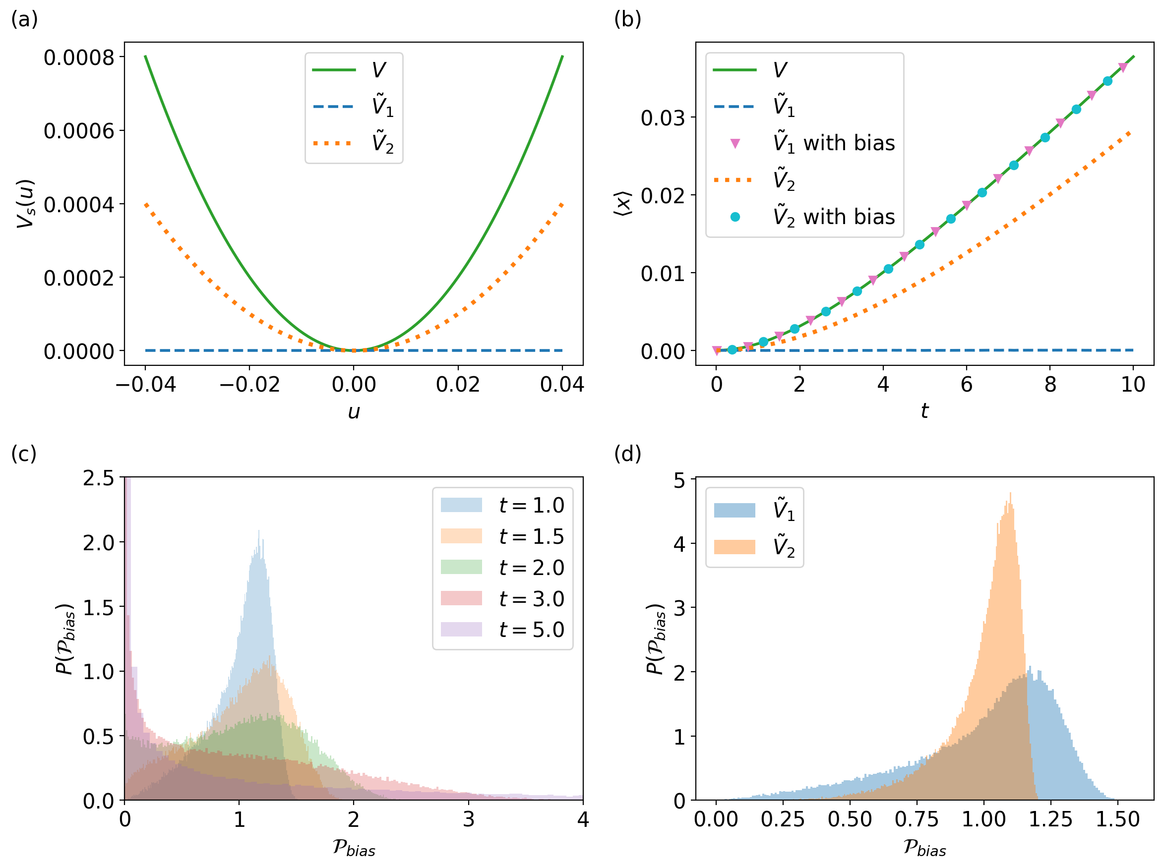
In this example, the aim is to predict the behavior of this system from a particle undergoing Brownian motion, i.e., V~1=0subscript~𝑉10\tilde{V}_{1}=0 and an intermediate harmonic potential V~2subscript~𝑉2\tilde{V}_{2} with spring constant k~=1/2~𝑘12\tilde{k}=1/2. Figures 1(a)-(b) shows the three interparticle potentials considered as well as the results of the Langevin simulations for each system, together with the predictions based on Eq. (4). While the predictions and the validations are indistinguishable, the normalized histogram of the path probability ratio 𝒫bias𝒫/𝒫~subscript𝒫𝑏𝑖𝑎𝑠𝒫~𝒫\mathcal{P}_{bias}\coloneqq\mathcal{P}/\tilde{\mathcal{P}} in Figures 1(c)-(d), clearly show that these become more heavy-tailed with time for a given potential V~~𝑉\tilde{V}, or for a fixed time, as the difference between the potentials V𝑉V and V~~𝑉\tilde{V} become larger. On a practical level, heavier tails imply larger errors for the empirical averages of Eq. (4) for a fixed number of realizations of system S~~𝑆\tilde{S}. Quantifying a priori these estimates is therefore crucial to assess the accuracy of the predictions without the need of validations. This is precisely the goal of the next section.
Refer to caption
Figure 1: (a) Interparticle potentials for the simulated (V~1subscript~𝑉1\tilde{V}_{1} and V~2subscript~𝑉2\tilde{V}_{2}) and targeted (V𝑉V) systems. (b) Ensemble average of the displacement for the simulated (V~1subscript~𝑉1\tilde{V}_{1} and V~2subscript~𝑉2\tilde{V}_{2}) and targeted systems (V𝑉V), as well as the predictions from the first to the latter (V~1subscript~𝑉1\tilde{V}_{1} with bias and V~2subscript~𝑉2\tilde{V}_{2} with bias). (c) Time evolution of the probability density for 𝒫biassubscript𝒫𝑏𝑖𝑎𝑠\mathcal{P}_{bias} from V~1subscript~𝑉1\tilde{V}_{1} to V𝑉V. (d) Comparison between the probability distribution of 𝒫biassubscript𝒫𝑏𝑖𝑎𝑠\mathcal{P}_{bias} at t=1𝑡1t=1 from V~1subscript~𝑉1\tilde{V}_{1} to V𝑉V and from V~2subscript~𝑉2\tilde{V}_{2} to V𝑉V. Parameters are chosen as N=1𝑁1N=1, η=5𝜂5\eta=5, β=104𝛽superscript104\beta=10^{4}, V~s1(u)=0subscript~𝑉𝑠1𝑢0\tilde{V}_{s1}(u)=0, V~s2(u)=14u2subscript~𝑉𝑠2𝑢14superscript𝑢2\tilde{V}_{s2}(u)=\frac{1}{4}u^{2}, Vs(u)=12u2subscript𝑉𝑠𝑢12superscript𝑢2V_{s}(u)=\frac{1}{2}u^{2}, NR=105subscript𝑁𝑅superscript105N_{R}=10^{5}.

3 Uncertainty Quantification

From Eq. (4) it is immediate that eβbiasS~=1subscriptdelimited-⟨⟩superscript𝑒𝛽subscript𝑏𝑖𝑎𝑠~𝑆1\left\langle e^{-\beta\mathcal{I}_{bias}}\right\rangle_{\tilde{S}}=1. Although this identity is exactly satisfied for the exact probability density, an empirical average, i.e., 𝒩r=1NR1NReβbias,r𝒩superscriptsubscript𝑟1subscript𝑁𝑅1subscript𝑁𝑅superscript𝑒𝛽subscript𝑏𝑖𝑎𝑠𝑟\mathcal{N}\coloneqq\sum_{r=1}^{N_{R}}\frac{1}{N_{R}}e^{-\beta\mathcal{I}_{bias,r}}, where NRsubscript𝑁𝑅N_{R} is the number of realizations, may deviate from 1 if insufficient samples are used. In general, more realizations will be needed the further apart systems/processes S~~𝑆\tilde{S} and S𝑆S are, as noted in the previous section. Such a distance can be measured by means of the Kullback-Leibler divergence, or relative entropy, between two probability distributions 𝒫~~𝒫\mathcal{\tilde{P}}, and 𝒫𝒫\mathcal{P}, which, in this case, is equal to

DKL(𝒫~𝒫)=log𝒫~𝒫S~=βIbiasS~.subscript𝐷𝐾𝐿conditional~𝒫𝒫subscriptdelimited-⟨⟩~𝒫𝒫~𝑆𝛽subscriptdelimited-⟨⟩subscript𝐼𝑏𝑖𝑎𝑠~𝑆D_{KL}\left(\tilde{\mathcal{P}}\|\mathcal{P}\right)=\left\langle\log\frac{\tilde{\mathcal{P}}}{\mathcal{P}}\right\rangle_{\tilde{S}}=\beta\langle{I}_{bias}\rangle_{\tilde{S}}. (6)

In practice, we will quantify the uncertainty of our predictions (for general observables 𝒪𝒪\mathcal{O}) using the standard error of the mean of 𝒫bias𝒫/𝒫~=eβbiassubscript𝒫𝑏𝑖𝑎𝑠𝒫~𝒫superscript𝑒𝛽subscript𝑏𝑖𝑎𝑠\mathcal{P}_{bias}\coloneqq\mathcal{P}/\tilde{\mathcal{P}}=e^{-\beta\mathcal{I}_{bias}}

σ𝒩=σ𝒫biasNR,subscript𝜎𝒩subscript𝜎subscript𝒫𝑏𝑖𝑎𝑠subscript𝑁𝑅\sigma_{\mathcal{N}}=\frac{\sigma_{\mathcal{P}_{bias}}}{\sqrt{N_{R}}}, (7)

where σ𝒫bias2subscriptsuperscript𝜎2subscript𝒫𝑏𝑖𝑎𝑠\sigma^{2}_{\mathcal{P}_{bias}} is the variance of 𝒫biassubscript𝒫𝑏𝑖𝑎𝑠\mathcal{P}_{bias}, and 𝒩=r=1NR1NR𝒫bias,r𝒩superscriptsubscript𝑟1subscript𝑁𝑅1subscript𝑁𝑅subscript𝒫𝑏𝑖𝑎𝑠𝑟\mathcal{N}=\sum_{r=1}^{N_{R}}\frac{1}{N_{R}}\mathcal{P}_{bias,r}. We use this standard error σ𝒩subscript𝜎𝒩\sigma_{\mathcal{N}} as an estimate for |𝒩1|𝒩1\left|\mathcal{N}-1\right|.

3.1 Linear uncertainty propagation estimate

The simplest approach to compute σ𝒫bias2subscriptsuperscript𝜎2subscript𝒫𝑏𝑖𝑎𝑠\sigma^{2}_{\mathcal{P}_{bias}} is to consider the time-discretized evaluation of 𝒫biassubscript𝒫𝑏𝑖𝑎𝑠\mathcal{P}_{bias} as a nonlinear function of Δξn=ξin+1ξinΔsuperscript𝜉𝑛subscriptsuperscript𝜉𝑛1𝑖subscriptsuperscript𝜉𝑛𝑖\Delta\xi^{n}=\xi^{n+1}_{i}-\xi^{n}_{i}, where the indices i𝑖i and n𝑛n here refer to the degrees of freedom i=1,,Nd𝑖1𝑁𝑑i=1,...,Nd (d𝑑d is the dimension of the problem), and discrete time tnsuperscript𝑡𝑛t^{n}, respectively, and to use the classical formulas for propagation of uncertainty [31, Chapter 3], i.e.,

σ𝒫bias2=i=1Ndn=0nT1(𝒫biasΔξin|Δ𝝃=𝟎)2σΔξin2=i=1Ndn=0nT1(𝒫biasΔξin|Δ𝝃=𝟎)2Δt.subscriptsuperscript𝜎2subscript𝒫𝑏𝑖𝑎𝑠superscriptsubscript𝑖1𝑁𝑑superscriptsubscript𝑛0subscript𝑛𝑇1superscriptevaluated-atsubscript𝒫𝑏𝑖𝑎𝑠Δsubscriptsuperscript𝜉𝑛𝑖Δ𝝃02subscriptsuperscript𝜎2Δsubscriptsuperscript𝜉𝑛𝑖superscriptsubscript𝑖1𝑁𝑑superscriptsubscript𝑛0subscript𝑛𝑇1superscriptevaluated-atsubscript𝒫𝑏𝑖𝑎𝑠Δsubscriptsuperscript𝜉𝑛𝑖Δ𝝃02Δ𝑡\sigma^{2}_{\mathcal{P}_{bias}}=\sum_{i=1}^{Nd}\sum_{n=0}^{n_{T}-1}\left(\frac{\partial\mathcal{P}_{bias}}{\partial\Delta\xi^{n}_{i}}\Big{|}_{\Delta\bm{\xi}=\mathbf{0}}\right)^{2}\sigma^{2}_{\Delta\xi^{n}_{i}}=\sum_{i=1}^{Nd}\sum_{n=0}^{n_{T}-1}\left(\frac{\partial\mathcal{P}_{bias}}{\partial\Delta\xi^{n}_{i}}\Big{|}_{\Delta\bm{\xi}=\mathbf{0}}\right)^{2}\Delta t. (8)

Here, we have made use of the fact that ΔξinΔsubscriptsuperscript𝜉𝑛𝑖\Delta\xi^{n}_{i} are uncorrelated, and σΔξin2=Δtsubscriptsuperscript𝜎2Δsubscriptsuperscript𝜉𝑛𝑖Δ𝑡\sigma^{2}_{\Delta\xi^{n}_{i}}=\Delta t. The notation |Δ𝝃=𝟎\Big{|}_{\Delta\bm{\xi}=\mathbf{0}} is used to denote that the partial derivatives are evaluated at the mean value of Δ𝝃Δ𝝃\Delta\bm{\xi}, which is zero.

As discussed in detail in A and B, 𝒫biassubscript𝒫𝑏𝑖𝑎𝑠\mathcal{P}_{bias} may be expressed using the Itô interpretation as

𝒫bias=exp[β4ηj=1Ndm=0nT1Vbias(𝐱m)xjm[Vbias(𝐱m)xjmΔt2σΔξjm]],withxjm=xj0+p=0m1Δxjp,Δxjp=xjp+1xjpandΔxjp=V~(𝐱p)xpjΔtη+σηΔξjp,formulae-sequencesubscript𝒫𝑏𝑖𝑎𝑠𝛽4𝜂superscriptsubscript𝑗1𝑁𝑑superscriptsubscript𝑚0subscript𝑛𝑇1subscript𝑉𝑏𝑖𝑎𝑠superscript𝐱𝑚superscriptsubscript𝑥𝑗𝑚delimited-[]subscript𝑉𝑏𝑖𝑎𝑠superscript𝐱𝑚superscriptsubscript𝑥𝑗𝑚Δ𝑡2𝜎Δsubscriptsuperscript𝜉𝑚𝑗formulae-sequencewithsubscriptsuperscript𝑥𝑚𝑗subscriptsuperscript𝑥0𝑗superscriptsubscript𝑝0𝑚1Δsubscriptsuperscript𝑥𝑝𝑗Δsubscriptsuperscript𝑥𝑝𝑗subscriptsuperscript𝑥𝑝1𝑗subscriptsuperscript𝑥𝑝𝑗andΔsubscriptsuperscript𝑥𝑝𝑗~𝑉superscript𝐱𝑝superscriptsubscript𝑥𝑝𝑗Δ𝑡𝜂𝜎𝜂Δsubscriptsuperscript𝜉𝑝𝑗\begin{split}&\mathcal{P}_{bias}=\exp\left[-\frac{\beta}{4\eta}\sum_{j=1}^{Nd}\sum_{m=0}^{n_{T}-1}\frac{\partial V_{bias}(\mathbf{x}^{m})}{\partial x_{j}^{m}}\left[\frac{\partial V_{bias}(\mathbf{x}^{m})}{\partial x_{j}^{m}}\Delta t-2\sqrt{\sigma}\Delta\xi^{m}_{j}\right]\right],\quad\text{with}\\ &x^{m}_{j}=x^{0}_{j}+\sum_{p=0}^{m-1}\Delta x^{p}_{j},\quad\Delta x^{p}_{j}=x^{p+1}_{j}-x^{p}_{j}\quad\text{and}\quad\Delta x^{p}_{j}=-\frac{\partial\tilde{V}(\mathbf{x}^{p})}{\partial x_{p}^{j}}\frac{\Delta t}{\eta}+\frac{\sqrt{\sigma}}{\eta}\Delta\xi^{p}_{j},\end{split} (9)

where σ=2kBTη𝜎2subscript𝑘𝐵𝑇𝜂\sigma=2k_{B}T\eta.

Noting that 𝒫biassubscript𝒫𝑏𝑖𝑎𝑠\mathcal{P}_{bias} depends on ΔξinΔsubscriptsuperscript𝜉𝑛𝑖\Delta\xi^{n}_{i} directly and through xjmsubscriptsuperscript𝑥𝑚𝑗x^{m}_{j} for m>n𝑚𝑛m>n, one obtains for the simplest case of V~=0~𝑉0\tilde{V}=0 that

𝒫biasΔξin=𝒫bias[β4η(j=1Ndm=n+1NT12Vbiasxjm2VbiasxjmximσηΔtVbiasxin2σ)].subscript𝒫𝑏𝑖𝑎𝑠Δsubscriptsuperscript𝜉𝑛𝑖subscript𝒫𝑏𝑖𝑎𝑠delimited-[]𝛽4𝜂superscriptsubscript𝑗1𝑁𝑑superscriptsubscript𝑚𝑛1subscript𝑁𝑇12subscript𝑉𝑏𝑖𝑎𝑠subscriptsuperscript𝑥𝑚𝑗superscript2subscript𝑉𝑏𝑖𝑎𝑠superscriptsubscript𝑥𝑗𝑚superscriptsubscript𝑥𝑖𝑚𝜎𝜂Δ𝑡subscript𝑉𝑏𝑖𝑎𝑠superscriptsubscript𝑥𝑖𝑛2𝜎\frac{\partial\mathcal{P}_{bias}}{\partial\Delta\xi^{n}_{i}}=\mathcal{P}_{bias}\left[-\frac{\beta}{4\eta}\left(\sum_{j=1}^{Nd}\sum_{m=n+1}^{N_{T}-1}2\frac{\partial V_{bias}}{\partial x^{m}_{j}}\frac{\partial^{2}V_{bias}}{\partial x_{j}^{m}\partial x_{i}^{m}}\frac{\sqrt{\sigma}}{\eta}\Delta t-\frac{\partial V_{bias}}{\partial x_{i}^{n}}2\sqrt{\sigma}\right)\right]. (10)

For such a case, the variance of 𝒫biassubscript𝒫𝑏𝑖𝑎𝑠\mathcal{P}_{bias} may then be easily computed as

σ𝒫bias2=β2η𝒫bias2i=1Ndn=0nT1[Vbiasxinj=1Nm=n+1nT1Vbiasxjm2VbiasxjmximΔtη]2Δt|Δ𝝃=𝟎.subscriptsuperscript𝜎2subscript𝒫𝑏𝑖𝑎𝑠evaluated-at𝛽2𝜂superscriptsubscript𝒫𝑏𝑖𝑎𝑠2superscriptsubscript𝑖1𝑁𝑑superscriptsubscript𝑛0subscript𝑛𝑇1superscriptdelimited-[]subscript𝑉𝑏𝑖𝑎𝑠superscriptsubscript𝑥𝑖𝑛superscriptsubscript𝑗1𝑁superscriptsubscript𝑚𝑛1subscript𝑛𝑇1subscript𝑉𝑏𝑖𝑎𝑠superscriptsubscript𝑥𝑗𝑚superscript2subscript𝑉𝑏𝑖𝑎𝑠superscriptsubscript𝑥𝑗𝑚superscriptsubscript𝑥𝑖𝑚Δ𝑡𝜂2Δ𝑡Δ𝝃0\sigma^{2}_{\mathcal{P}_{bias}}=\frac{\beta}{2\eta}\mathcal{P}_{bias}^{2}\sum_{i=1}^{Nd}\sum_{n=0}^{n_{T}-1}\left[\frac{\partial V_{bias}}{\partial x_{i}^{n}}-\sum_{j=1}^{N}\sum_{m=n+1}^{n_{T}-1}\frac{\partial V_{bias}}{\partial x_{j}^{m}}\frac{\partial^{2}V_{bias}}{\partial x_{j}^{m}\partial x_{i}^{m}}\frac{\Delta t}{\eta}\right]^{2}\Delta t\Bigg{|}_{\Delta\bm{\xi}=\mathbf{0}}. (11)

As will be seen later on in Fig. 2 by means of an example, this uncertainty propagation method, albeit simple for V~=0~𝑉0\tilde{V}=0, does not capture well the variance of 𝒫biassubscript𝒫𝑏𝑖𝑎𝑠\mathcal{P}_{bias} even for very simple physical systems. This is likely due to the importance of nonlinear effects induced by the exponential of 𝒫biassubscript𝒫𝑏𝑖𝑎𝑠\mathcal{P}_{bias}. Furthermore, its generalization to simulated systems with V~0~𝑉0\tilde{V}\neq 0 is rather intricate, due to the many nested sums that this would require.

3.2 Nonlinear uncertainty quantification estimate

To resolve the above two issues, we resort instead to perform a linear approximation to the bias potential gradient in the exponent of 𝒫biassubscript𝒫𝑏𝑖𝑎𝑠\mathcal{P}_{bias} to then estimate σ𝒫bias2subscriptsuperscript𝜎2subscript𝒫𝑏𝑖𝑎𝑠\sigma^{2}_{\mathcal{P}_{bias}} directly as 𝒫bias2S~𝒫biasS~2subscriptdelimited-⟨⟩superscriptsubscript𝒫𝑏𝑖𝑎𝑠2~𝑆superscriptsubscriptdelimited-⟨⟩subscript𝒫𝑏𝑖𝑎𝑠~𝑆2\langle\mathcal{P}_{bias}^{2}\rangle_{\tilde{S}}-\langle\mathcal{P}_{bias}\rangle_{\tilde{S}}^{2}. Specifically, we expand the bias potential gradient linearly from a reference trajectory 𝐱r(t)subscript𝐱𝑟𝑡\mathbf{x}_{r}(t) as

Vbias(𝐱,t)=Vbias|𝐱r(t)+Vbias|𝐱r(t)δ𝐱+O(δ𝐱2),subscript𝑉𝑏𝑖𝑎𝑠𝐱𝑡evaluated-atsubscript𝑉𝑏𝑖𝑎𝑠subscript𝐱𝑟𝑡evaluated-atsubscript𝑉𝑏𝑖𝑎𝑠subscript𝐱𝑟𝑡𝛿𝐱𝑂superscriptnorm𝛿𝐱2\nabla V_{bias}(\mathbf{x},t)=\left.\nabla V_{bias}\right|_{\mathbf{x}_{r}(t)}+\left.\nabla\nabla V_{bias}\right|_{\mathbf{x}_{r}(t)}\delta\mathbf{x}+O(\left\|\delta\mathbf{x}\right\|^{2}), (12)

where δ𝐱=𝐱𝐱r𝛿𝐱𝐱subscript𝐱𝑟\delta\mathbf{x}=\mathbf{x}-\mathbf{x}_{r}. Similarly, the noise term in the Langevin equations associated to system S~~𝑆\tilde{S} may be approximated as

σΔ𝝃n=η(𝐱n+1𝐱n)+V~(𝐱n,tn)Δt=η(Δ𝐱rn+δ𝐱n+1δ𝐱n)+V~|𝐱rnΔt+V~|𝐱rnδ𝐱nΔt+O(δ𝐱2Δt),𝜎Δsuperscript𝝃𝑛𝜂superscript𝐱𝑛1superscript𝐱𝑛~𝑉superscript𝐱𝑛superscript𝑡𝑛Δ𝑡𝜂Δsubscriptsuperscript𝐱𝑛𝑟𝛿superscript𝐱𝑛1𝛿superscript𝐱𝑛evaluated-at~𝑉superscriptsubscript𝐱𝑟𝑛Δ𝑡evaluated-at~𝑉superscriptsubscript𝐱𝑟𝑛𝛿superscript𝐱𝑛Δ𝑡𝑂superscriptdelimited-∥∥𝛿𝐱2Δ𝑡\begin{split}\sqrt{\sigma}\Delta\bm{\xi}^{n}&=\eta\left(\mathbf{x}^{n+1}-\mathbf{x}^{n}\right)+\nabla\tilde{V}(\mathbf{x}^{n},t^{n})\Delta t\\ &=\eta\left(\Delta\mathbf{x}^{n}_{r}+\delta\mathbf{x}^{n+1}-\delta\mathbf{x}^{n}\right)+\left.\nabla\tilde{V}\right|_{\mathbf{x}_{r}^{n}}\Delta t+\left.\nabla\nabla\tilde{V}\right|_{\mathbf{x}_{r}^{n}}\delta\mathbf{x}^{n}\Delta t+O(\left\|\delta\mathbf{x}\right\|^{2}\Delta t),\end{split} (13)

where we have used an Itô representation for the discretized equations and defined Δ𝐱rn=𝐱rn+1𝐱rnΔsubscriptsuperscript𝐱𝑛𝑟subscriptsuperscript𝐱𝑛1𝑟subscriptsuperscript𝐱𝑛𝑟\Delta\mathbf{x}^{n}_{r}=\mathbf{x}^{n+1}_{r}-\mathbf{x}^{n}_{r}. Using the above two approximations, and the change of variables δ𝐲n=(η/σΔt)δ𝐱n𝛿superscript𝐲𝑛𝜂𝜎Δ𝑡𝛿superscript𝐱𝑛\delta\mathbf{y}^{n}=\left(\eta/\sqrt{\sigma\Delta t}\right)\delta\mathbf{x}^{n}, introduced for convenience, the exponents in 𝒫biassubscript𝒫𝑏𝑖𝑎𝑠\mathcal{P}_{bias} and 𝒫~~𝒫\tilde{\mathcal{P}} have a quadratic form in δ𝐲n𝛿superscript𝐲𝑛\delta\mathbf{y}^{n}. As a result, both 𝒫biasS~subscriptdelimited-⟨⟩subscript𝒫𝑏𝑖𝑎𝑠~𝑆\langle\mathcal{P}_{bias}\rangle_{\tilde{S}} and 𝒫bias2S~subscriptdelimited-⟨⟩superscriptsubscript𝒫𝑏𝑖𝑎𝑠2~𝑆\langle\mathcal{P}_{bias}^{2}\rangle_{\tilde{S}} may be computed analytically. These derivations are quite involved and are therefore relayed to C. The resulting expression for 𝒫biasS~subscriptdelimited-⟨⟩subscript𝒫𝑏𝑖𝑎𝑠~𝑆\langle\mathcal{P}_{bias}\rangle_{\tilde{S}} is

𝒫biasS~=1det𝐀e12𝐛T𝐀1𝐛+c.subscriptdelimited-⟨⟩subscript𝒫𝑏𝑖𝑎𝑠~𝑆1𝐀superscript𝑒12superscript𝐛Tsuperscript𝐀1𝐛𝑐\langle\mathcal{P}_{bias}\rangle_{\tilde{S}}=\frac{1}{\sqrt{\det\mathbf{A}}}e^{\frac{1}{2}\mathbf{b}^{\text{T}}\mathbf{A}^{-1}\mathbf{b}+c}. (14)

Here, c𝑐c is a constant defined as,

c=12σn=0nT1ηΔ𝐱rnΔt+V|𝐱rn2Δt,c=-\frac{1}{2\sigma}\sum_{n=0}^{n_{T}-1}\left\|\eta\frac{\Delta\mathbf{x}^{n}_{r}}{\Delta t}+\left.\nabla V\right|_{\mathbf{x}_{r}^{n}}\right\|^{2}\Delta t, (15)

the vector 𝐛𝐛\mathbf{b} consists of nTsubscript𝑛𝑇n_{T} small Nd𝑁𝑑Nd-dimensional vectors,

𝐛=(𝐛1𝐛2𝐛nT),𝐛matrixsuperscript𝐛1superscript𝐛2superscript𝐛subscript𝑛𝑇\begin{split}\mathbf{b}=\begin{pmatrix}\mathbf{b}^{1}\\ \mathbf{b}^{2}\\ \vdots\\ \mathbf{b}^{n_{T}}\end{pmatrix},\end{split} (16)

with

𝐛n={Δtσ[ΔtηV|𝐱rn(ηΔ𝐱rnΔt+V|𝐱rn)Δ(ηΔ𝐱rn1Δt+V|𝐱rn1)],n<nTΔtσ(ηΔ𝐱rnT1Δt+V|𝐱rnT1),n=nT\begin{split}\mathbf{b}^{n}=\left\{\begin{aligned} &-\sqrt{\frac{\Delta t}{\sigma}}\left[\frac{\Delta t}{\eta}\left.\nabla\nabla V\right|_{\mathbf{x}_{r}^{n}}\left(\eta\frac{\Delta\mathbf{x}^{n}_{r}}{\Delta t}+\left.\nabla V\right|_{\mathbf{x}_{r}^{n}}\right)-\Delta\left(\eta\frac{\Delta\mathbf{x}^{n-1}_{r}}{\Delta t}+\left.\nabla V\right|_{\mathbf{x}_{r}^{n-1}}\right)\right],\quad&&n<n_{T}\\ &-\sqrt{\frac{\Delta t}{\sigma}}\left(\eta\frac{\Delta\mathbf{x}^{n_{T}-1}_{r}}{\Delta t}+\left.\nabla V\right|_{\mathbf{x}_{r}^{n_{T}-1}}\right),\quad&&n=n_{T}\end{aligned}\right.\end{split} (17)

and the matrix 𝐀𝐀\mathbf{A} may be written as,

𝐀=(𝐀11𝐀12𝐀1nT𝐀21𝐀22𝐀2nT𝐀nT1𝐀nT2𝐀nTnT)𝐀matrixsuperscript𝐀11superscript𝐀12superscript𝐀1subscript𝑛𝑇superscript𝐀21superscript𝐀22superscript𝐀2subscript𝑛𝑇superscript𝐀subscript𝑛𝑇1superscript𝐀subscript𝑛𝑇2superscript𝐀subscript𝑛𝑇subscript𝑛𝑇\begin{split}\mathbf{A}&=\begin{pmatrix}\mathbf{A}^{11}&\mathbf{A}^{12}&\cdots&\mathbf{A}^{1n_{T}}\\ \mathbf{A}^{21}&\mathbf{A}^{22}&\cdots&\mathbf{A}^{2n_{T}}\\ \vdots&\vdots&\ddots&\vdots\\ \mathbf{A}^{n_{T}1}&\mathbf{A}^{n_{T}2}&\cdots&\mathbf{A}^{n_{T}n_{T}}\end{pmatrix}\end{split} (18)

with each Nd×Nd𝑁𝑑𝑁𝑑Nd\times Nd matrix block defined as,

𝐀pq={𝐈+𝚪n𝚪n,(p,q)=(n,n) with n=1,,nT1𝚪n,(p,q)=(n+1,n) or (n,n+1) with n=1,,nT1𝐈,(p,q)=(nT,nT)𝟎,otherwise\begin{split}\mathbf{A}^{pq}&=\left\{\begin{aligned} &\mathbf{I}+\mathbf{\Gamma}^{n}\mathbf{\Gamma}^{n},\quad\quad&&(p,q)=(n,n)\text{ with }n=1,\cdots,n_{T}-1\\ &-\mathbf{\Gamma}^{n},&&(p,q)=(n+1,n)\text{ or }(n,n+1)\text{ with }n=1,\cdots,n_{T}-1\\ &\mathbf{I},&&(p,q)=(n_{T},n_{T})\\ &\mathbf{0},&&\text{otherwise}\\ \end{aligned}\right.\end{split} (19)

with

𝚪n=𝐈1ηV|𝐱rnΔt.superscript𝚪𝑛𝐈evaluated-at1𝜂𝑉superscriptsubscript𝐱𝑟𝑛Δ𝑡\mathbf{\Gamma}^{n}=\mathbf{I}-\frac{1}{\eta}\left.\nabla\nabla V\right|_{\mathbf{x}_{r}^{n}}\Delta t. (20)

The matrix 𝐀𝐀\mathbf{A} is thus symmetric. Remarkably, as detailed in C, it may be shown that the equations det(𝐀)=1𝐀1\det(\mathbf{A})=1 and 𝐛T𝐀1𝐛=2csuperscript𝐛Tsuperscript𝐀1𝐛2𝑐\mathbf{b}^{\text{T}}\mathbf{A}^{-1}\mathbf{b}=-2c are identically satisfied in this discretized setting leading to 𝒫biasS~=1subscriptdelimited-⟨⟩subscript𝒫𝑏𝑖𝑎𝑠~𝑆1\langle\mathcal{P}_{bias}\rangle_{\tilde{S}}=1. We remark that in these derivations, the ensemble average for 𝒫biasS~subscriptdelimited-⟨⟩subscript𝒫𝑏𝑖𝑎𝑠~𝑆\langle\mathcal{P}_{bias}\rangle_{\tilde{S}} is analytically computed, i.e., it does not result from an empirical average.

As for 𝒫bias2S~subscriptdelimited-⟨⟩superscriptsubscript𝒫𝑏𝑖𝑎𝑠2~𝑆\langle\mathcal{P}_{bias}^{2}\rangle_{\tilde{S}}, this reads

𝒫bias2S~=1det(𝐀sq)e12𝐛sqT𝐀sq1𝐛sq+csq,subscriptdelimited-⟨⟩superscriptsubscript𝒫𝑏𝑖𝑎𝑠2~𝑆1subscript𝐀𝑠𝑞superscript𝑒12subscriptsuperscript𝐛T𝑠𝑞superscriptsubscript𝐀𝑠𝑞1subscript𝐛𝑠𝑞subscript𝑐𝑠𝑞\langle\mathcal{P}_{bias}^{2}\rangle_{\tilde{S}}=\frac{1}{\sqrt{\det(\mathbf{A}_{sq})}}e^{\frac{1}{2}\mathbf{b}^{\text{T}}_{sq}\mathbf{A}_{sq}^{-1}\mathbf{b}_{sq}+c_{sq}}, (21)

where the coefficients 𝐀sqsubscript𝐀𝑠𝑞\mathbf{A}_{sq}, 𝐛sqsubscript𝐛𝑠𝑞\mathbf{b}_{sq} and csqsubscript𝑐𝑠𝑞c_{sq} can be expressed as,

𝐀sq=2𝐀𝐀~,subscript𝐀𝑠𝑞2𝐀~𝐀\displaystyle\mathbf{A}_{sq}=2\mathbf{A}-\tilde{\mathbf{A}}, (22)
𝐛sq=2𝐛𝐛~,subscript𝐛𝑠𝑞2𝐛~𝐛\displaystyle\mathbf{b}_{sq}=2\mathbf{b}-\tilde{\mathbf{b}}, (23)
csq=2cc~.subscript𝑐𝑠𝑞2𝑐~𝑐\displaystyle c_{sq}=2c-\tilde{c}. (24)

Here, 𝐀~~𝐀\tilde{\mathbf{A}}, 𝐛~~𝐛\tilde{\mathbf{b}} and c~~𝑐\tilde{c} are the defined as the analogues of 𝐀𝐀\mathbf{A}, 𝐛𝐛\mathbf{b}, and c𝑐c, respectively, with the potential V𝑉V replaced by V~~𝑉\tilde{V}.

Therefore, the resulting expression for the variance of 𝒫biassubscript𝒫𝑏𝑖𝑎𝑠\mathcal{P}_{bias} is,

σ𝒫bias2=𝒫bias2S~𝒫biasS~2=1det(𝐀sq)e12𝐛sqT𝐀sq1𝐛sq+csq1.subscriptsuperscript𝜎2subscript𝒫𝑏𝑖𝑎𝑠subscriptdelimited-⟨⟩superscriptsubscript𝒫𝑏𝑖𝑎𝑠2~𝑆superscriptsubscriptdelimited-⟨⟩subscript𝒫𝑏𝑖𝑎𝑠~𝑆21subscript𝐀𝑠𝑞superscript𝑒12subscriptsuperscript𝐛T𝑠𝑞superscriptsubscript𝐀𝑠𝑞1subscript𝐛𝑠𝑞subscript𝑐𝑠𝑞1\begin{split}\sigma^{2}_{\mathcal{P}_{bias}}&=\left<\mathcal{P}_{bias}^{2}\right>_{\tilde{S}}-\left<\mathcal{P}_{bias}\right>_{\tilde{S}}^{2}\\ &=\frac{1}{\sqrt{\det(\mathbf{A}_{sq})}}e^{\frac{1}{2}\mathbf{b}^{\text{T}}_{sq}\mathbf{A}_{sq}^{-1}\mathbf{b}_{sq}+c_{sq}}-1.\end{split} (25)

The details of its implementation are detailed in Algorithm 2.

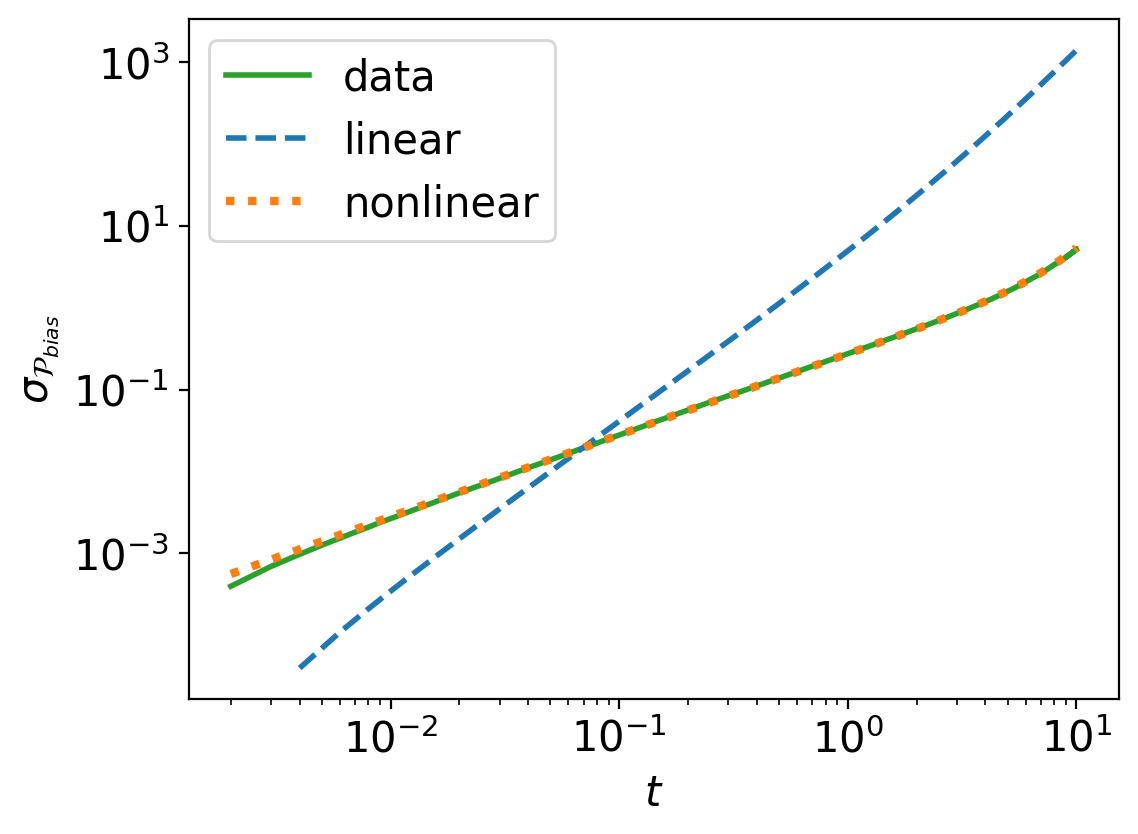
To illustrate the improved performance of this estimate compared to the classical uncertainty propagation approach, consider the single one degree of freedom system discussed at the end of Section 2 with V~=0~𝑉0\tilde{V}=0. Figure 2 shows the value of σ𝒫biassubscript𝜎subscript𝒫𝑏𝑖𝑎𝑠\sigma_{\mathcal{P}_{bias}} as a function of time, directly obtained from numerical simulations, together with the estimates given by Eq. (11) and Eq. (25). As it may there be observed, the difference in accuracy is striking, even for this rather simple example. Consequently, the later examples will make use of the nonlinear propagation of uncertainty strategy described in this section.
Refer to caption
Figure 2: Prediction of the standard deviation of 𝒫biassubscript𝒫𝑏𝑖𝑎𝑠\mathcal{P}_{bias} with the linear (blue dashed line) and nonlinear (orange dotted line) uncertainty estimates, together with σ𝒫biassubscript𝜎subscript𝒫𝑏𝑖𝑎𝑠\sigma_{\mathcal{P}_{bias}}, as directly computed from simulation data (green solid line). The simulation parameters are N=1𝑁1N=1, NR=105subscript𝑁𝑅superscript105N_{R}=10^{5}, kBT=104subscript𝑘𝐵𝑇superscript104k_{B}T=10^{-4}, η=5𝜂5\eta=5, vp=0.01subscript𝑣𝑝0.01v_{p}=0.01, Δt=103Δ𝑡superscript103\Delta t=10^{-3}, from Brownian motion to quadratic potential with k=1𝑘1k=1. For the nonlinear uncertainty quantification estimates, the time discretization used is nT=100subscript𝑛𝑇100n_{T}=100 and the reference trajectory is chosen as 𝐱r=𝟎subscript𝐱𝑟0\mathbf{x}_{r}=\mathbf{0}.

We remark that the accuracy of the uncertainty quantification (UQ) estimates here derived will strongly depend on the form of the bias potential that the trajectories explore. Equation (25) is nominally exact for a quadratic bias (such as the one used in Fig. 2), though it is expected to only give an estimate for general potentials. In the example of Section 4, quartic potentials will be considered, while Section 5 will examine systems with Hertzian and Lennard-Jones potentials. These last two potentials strongly deviate from quadratic, with the Hertzian not even displaying a unique minimum, and will thus allow us to explore the degree of accuracy of these estimates for a wide range of systems.

1       Choose a reference trajectory 𝐱r(t)subscript𝐱𝑟𝑡\mathbf{x}_{r}(t) for all selected t<T𝑡𝑇t<T at which to estimate the uncertainty do
2             Set timestep as Δt=t/nTΔ𝑡𝑡subscript𝑛𝑇\Delta t=t/n_{T}; for all n𝑛n from 00 to nTsubscript𝑛𝑇n_{T} do
3                   τn=nΔtsuperscript𝜏𝑛𝑛Δ𝑡\tau^{n}=n\Delta t; Compute 𝐱rnsuperscriptsubscript𝐱𝑟𝑛\mathbf{x}_{r}^{n}, 𝐱˙rnsuperscriptsubscript˙𝐱𝑟𝑛\dot{\mathbf{x}}_{r}^{n}, V|𝐱rnevaluated-at𝑉superscriptsubscript𝐱𝑟𝑛\left.\nabla V\right|_{\mathbf{x}_{r}^{n}}, V~|𝐱rnevaluated-at~𝑉superscriptsubscript𝐱𝑟𝑛\left.\nabla\tilde{V}\right|_{\mathbf{x}_{r}^{n}}, V|𝐱rnevaluated-at𝑉superscriptsubscript𝐱𝑟𝑛\left.\nabla\nabla V\right|_{\mathbf{x}_{r}^{n}}, V~|𝐱rnevaluated-at~𝑉superscriptsubscript𝐱𝑟𝑛\left.\nabla\nabla\tilde{V}\right|_{\mathbf{x}_{r}^{n}} at time τnsuperscript𝜏𝑛\tau^{n};
4            Compute c𝑐c and csqsubscript𝑐𝑠𝑞c_{sq} as in Eqs. (15) and (24); Initialize 𝐛𝐛\mathbf{b} and 𝐛sqsubscript𝐛𝑠𝑞\mathbf{b}_{sq} as zero vectors with size NdnT𝑁𝑑subscript𝑛𝑇Ndn_{T}, 𝐀𝐀\mathbf{A} and 𝐀sqsubscript𝐀𝑠𝑞\mathbf{A}_{sq} as zero matrices with size NdnT×NdnT𝑁𝑑subscript𝑛𝑇𝑁𝑑subscript𝑛𝑇Ndn_{T}\times Ndn_{T} for all n𝑛n from 111 to nT1subscript𝑛𝑇1n_{T}-1 do
5                   Compute vector components 𝐛nsuperscript𝐛𝑛\mathbf{b}^{n} and 𝐛sqnsubscriptsuperscript𝐛𝑛𝑠𝑞\mathbf{b}^{n}_{sq} as in Eqs. (16) and (23); Compute 𝚪nsuperscript𝚪𝑛\mathbf{\Gamma}^{n} and 𝚪~nsuperscript~𝚪𝑛\mathbf{\tilde{\Gamma}}^{n} as in Eq. (20); Compute matrix blocks 𝐀pqsuperscript𝐀𝑝𝑞\mathbf{A}^{pq} and 𝐀sqpqsuperscriptsubscript𝐀𝑠𝑞𝑝𝑞\mathbf{A}_{sq}^{pq} for (p,q)=(n,n),(n+1,n)𝑝𝑞𝑛𝑛𝑛1𝑛(p,q)=(n,n),(n+1,n) and (n,n+1)𝑛𝑛1(n,n+1) as in Eqs. (19) and (22);
6            Compute 𝐛nTsuperscript𝐛subscript𝑛𝑇\mathbf{b}^{n_{T}}, 𝐛sqnTsubscriptsuperscript𝐛subscript𝑛𝑇𝑠𝑞\mathbf{b}^{n_{T}}_{sq} as in Eqs. (16), (23) and 𝐀nTnTsuperscript𝐀subscript𝑛𝑇subscript𝑛𝑇\mathbf{A}^{n_{T}n_{T}}, 𝐀sqnTnTsubscriptsuperscript𝐀subscript𝑛𝑇subscript𝑛𝑇𝑠𝑞\mathbf{A}^{n_{T}n_{T}}_{sq} as in Eqs. (19), (22); Solve 𝐮sqsubscript𝐮𝑠𝑞\mathbf{u}_{sq} from 𝐀𝐬𝐪𝐮𝐬𝐪=𝐛𝐬𝐪subscript𝐀𝐬𝐪subscript𝐮𝐬𝐪subscript𝐛𝐬𝐪\mathbf{A_{sq}u_{sq}}=\mathbf{b_{sq}}; Compute 𝐛sqT𝐀sq1𝐛sq=𝐛sq𝐮sqsubscriptsuperscript𝐛T𝑠𝑞superscriptsubscript𝐀𝑠𝑞1subscript𝐛𝑠𝑞subscript𝐛𝑠𝑞subscript𝐮𝑠𝑞\mathbf{b}^{\text{T}}_{sq}\mathbf{A}_{sq}^{-1}\mathbf{b}_{sq}=\mathbf{b}_{sq}\cdot\mathbf{u}_{sq}; Compute det(𝐀sq)subscript𝐀𝑠𝑞\det\left(\mathbf{A}_{sq}\right); σ𝒫bias2(t)=1det(𝐀sq)exp(12𝐛sqT𝐀sq1𝐛sq+csq)1.subscriptsuperscript𝜎2subscript𝒫𝑏𝑖𝑎𝑠𝑡1subscript𝐀𝑠𝑞12subscriptsuperscript𝐛T𝑠𝑞superscriptsubscript𝐀𝑠𝑞1subscript𝐛𝑠𝑞subscript𝑐𝑠𝑞1\sigma^{2}_{\mathcal{P}_{bias}}(t)=\frac{1}{\sqrt{\det\left(\mathbf{A}_{sq}\right)}}\exp\left(\frac{1}{2}\mathbf{b}^{\text{T}}_{sq}\mathbf{A}_{sq}^{-1}\mathbf{b}_{sq}+c_{sq}\right)-1.
7      
Algorithm 2 Pseudo-code for nonlinear uncertainty quantification

3.3 Connection between the two strategies

While the two UQ approaches previously discussed in Sections 3.1 and 3.2 are quite distinct in their starting point and final conclusions, Eq. (11) may actually be recovered following the same strategy as for the nonlinear estimate under various simplifying assumptions. In particular, assuming 𝐱r(t)=𝟎subscript𝐱𝑟𝑡0\mathbf{x}_{r}(t)=\mathbf{0} (hence, Δ𝐱rn=𝟎Δsuperscriptsubscript𝐱𝑟𝑛0\Delta\mathbf{x}_{r}^{n}=\mathbf{0}, and δ𝐱n=𝐱n𝛿superscript𝐱𝑛superscript𝐱𝑛\delta\mathbf{x}^{n}=\mathbf{x}^{n}), V~=0~𝑉0\tilde{V}=0 (hence, V=Vbias𝑉subscript𝑉𝑏𝑖𝑎𝑠V=-V_{bias}), and only keeping linear terms in the integrand of biassubscript𝑏𝑖𝑎𝑠\mathcal{I}_{bias}, such integrand can be approximated as

Vbias(𝐱n,tn)(Vbias(𝐱n,tn)Δt2σΔ𝝃n)Vbias|𝐱rn=𝟎2Δt2Vbias|𝐱rn=𝟎[η(𝐱n+1𝐱n)Vbias|𝐱rn=𝟎𝐱nΔt].\begin{split}&\nabla V_{bias}(\mathbf{x}^{n},t^{n})\cdot\left(\nabla V_{bias}(\mathbf{x}^{n},t^{n})\Delta t-2\sqrt{\sigma}\Delta\bm{\xi}^{n}\right)\\ &\simeq\left\|\left.\nabla V_{bias}\right|_{\mathbf{x}_{r}^{n}=\mathbf{0}}\right\|^{2}\Delta t-2\left.\nabla V_{bias}\right|_{\mathbf{x}_{r}^{n}=\mathbf{0}}\cdot\left[\eta\left(\mathbf{x}^{n+1}-\mathbf{x}^{n}\right)-\left.\nabla\nabla V_{bias}\right|_{\mathbf{x}_{r}^{n}=\mathbf{0}}\mathbf{x}^{n}\Delta t\right].\end{split} (26)

Next, following the discrete Langevin equation for system S~~𝑆\tilde{S}, we replace in the above expression η(𝐱n+1𝐱n)=σΔ𝝃n𝜂superscript𝐱𝑛1superscript𝐱𝑛𝜎Δsuperscript𝝃𝑛\eta(\mathbf{x}^{n+1}-\mathbf{x}^{n})=\sqrt{\sigma}\Delta\bm{\xi}^{n}, and 𝐱n=m=0n1Δ𝐱m=m=0n1σηΔ𝝃msuperscript𝐱𝑛superscriptsubscript𝑚0𝑛1Δsuperscript𝐱𝑚superscriptsubscript𝑚0𝑛1𝜎𝜂Δsuperscript𝝃𝑚\mathbf{x}^{n}=\sum_{m=0}^{n-1}\Delta\mathbf{x}^{m}=\sum_{m=0}^{n-1}\frac{\sqrt{\sigma}}{\eta}\Delta\bm{\xi}^{m}. Furthermore, we note that expanding around 𝐱r=𝟎subscript𝐱𝑟0\mathbf{x}_{r}=\mathbf{0} is identical to expanding around Δ𝝃=𝟎Δ𝝃0\Delta\bm{\xi}=\mathbf{0}. Then, 𝒫biassubscript𝒫𝑏𝑖𝑎𝑠\mathcal{P}_{bias} can be written as a function of Δ𝝃Δ𝝃\Delta\bm{\xi} and 𝒫biasS~2subscriptsuperscriptdelimited-⟨⟩subscript𝒫𝑏𝑖𝑎𝑠2~𝑆\left<\mathcal{P}_{bias}\right>^{2}_{\tilde{S}} and 𝒫bias2S~subscriptdelimited-⟨⟩superscriptsubscript𝒫𝑏𝑖𝑎𝑠2~𝑆\left<\mathcal{P}_{bias}^{2}\right>_{\tilde{S}} may be computed analytically, giving (for details see D)

𝒫biasS~2exp[1σn=0nT1Vbias(𝐱n,tn)2Δt]|Δ𝝃=𝟎exp[Δtσn=0nT1(Vbias(𝐱n,tn)1ηm=n+1nT1Vbias(𝐱m,tm)Vbias(𝐱m,tm)Δt)2|Δ𝝃=𝟎]similar-to-or-equalssubscriptsuperscriptdelimited-⟨⟩subscript𝒫𝑏𝑖𝑎𝑠2~𝑆evaluated-at1𝜎superscriptsubscript𝑛0subscript𝑛𝑇1superscriptdelimited-∥∥subscript𝑉𝑏𝑖𝑎𝑠superscript𝐱𝑛superscript𝑡𝑛2Δ𝑡Δ𝝃0evaluated-atΔ𝑡𝜎superscriptsubscript𝑛0subscript𝑛𝑇1superscriptsubscript𝑉𝑏𝑖𝑎𝑠superscript𝐱𝑛superscript𝑡𝑛1𝜂superscriptsubscript𝑚𝑛1subscript𝑛𝑇1subscript𝑉𝑏𝑖𝑎𝑠superscript𝐱𝑚superscript𝑡𝑚subscript𝑉𝑏𝑖𝑎𝑠superscript𝐱𝑚superscript𝑡𝑚Δ𝑡2Δ𝝃0\begin{split}\left<\mathcal{P}_{bias}\right>^{2}_{\tilde{S}}&\simeq\left.\exp\left[-\frac{1}{\sigma}\sum_{n=0}^{n_{T}-1}\left\|\nabla V_{bias}(\mathbf{x}^{n},t^{n})\right\|^{2}\Delta t\right]\right|_{\Delta\bm{\xi}=\mathbf{0}}\\ &\quad\exp\left[\frac{\Delta t}{\sigma}\sum_{n=0}^{n_{T}-1}\left.\left(\nabla V_{bias}(\mathbf{x}^{n},t^{n})-\frac{1}{\eta}\sum_{m=n+1}^{n_{T}-1}\nabla\nabla V_{bias}(\mathbf{x}^{m},t^{m})\nabla V_{bias}(\mathbf{x}^{m},t^{m})\Delta t\right)^{2}\right|_{\Delta\bm{\xi}=\mathbf{0}}\right]\end{split} (27)
𝒫bias2S~exp[1σn=0nT1Vbias(𝐱n,tn)2Δt]|Δ𝝃=𝟎exp[2Δtσn=0nT1(Vbias(𝐱n,tn)1ηm=n+1nT1Vbias(𝐱m,tm)Vbias(𝐱m,tm)Δt)2|Δ𝝃=𝟎]similar-to-or-equalssubscriptdelimited-⟨⟩superscriptsubscript𝒫𝑏𝑖𝑎𝑠2~𝑆evaluated-at1𝜎superscriptsubscript𝑛0subscript𝑛𝑇1superscriptdelimited-∥∥subscript𝑉𝑏𝑖𝑎𝑠superscript𝐱𝑛superscript𝑡𝑛2Δ𝑡Δ𝝃0evaluated-at2Δ𝑡𝜎superscriptsubscript𝑛0subscript𝑛𝑇1superscriptsubscript𝑉𝑏𝑖𝑎𝑠superscript𝐱𝑛superscript𝑡𝑛1𝜂superscriptsubscript𝑚𝑛1subscript𝑛𝑇1subscript𝑉𝑏𝑖𝑎𝑠superscript𝐱𝑚superscript𝑡𝑚subscript𝑉𝑏𝑖𝑎𝑠superscript𝐱𝑚superscript𝑡𝑚Δ𝑡2Δ𝝃0\begin{split}\left<\mathcal{P}_{bias}^{2}\right>_{\tilde{S}}&\simeq\left.\exp\left[-\frac{1}{\sigma}\sum_{n=0}^{n_{T}-1}\left\|\nabla V_{bias}(\mathbf{x}^{n},t^{n})\right\|^{2}\Delta t\right]\right|_{\Delta\bm{\xi}=\mathbf{0}}\\ &\quad\exp\left[\frac{2\Delta t}{\sigma}\sum_{n=0}^{n_{T}-1}\left.\left(\nabla V_{bias}(\mathbf{x}^{n},t^{n})-\frac{1}{\eta}\sum_{m=n+1}^{n_{T}-1}\nabla\nabla V_{bias}(\mathbf{x}^{m},t^{m})\nabla V_{bias}(\mathbf{x}^{m},t^{m})\Delta t\right)^{2}\right|_{\Delta\bm{\xi}=\mathbf{0}}\right]\end{split} (28)

Finally, assuming that the second exponential terms in both 𝒫biasS~2subscriptsuperscriptdelimited-⟨⟩subscript𝒫𝑏𝑖𝑎𝑠2~𝑆\left<\mathcal{P}_{bias}\right>^{2}_{\tilde{S}} and 𝒫bias2S~subscriptdelimited-⟨⟩superscriptsubscript𝒫𝑏𝑖𝑎𝑠2~𝑆\left<\mathcal{P}_{bias}^{2}\right>_{\tilde{S}} are small, we approximate exp(x)1+xsimilar-to-or-equals𝑥1𝑥\exp\left(x\right)\simeq 1+x, obtaining the following expression for the variance of 𝒫biassubscript𝒫𝑏𝑖𝑎𝑠\mathcal{P}_{bias}

σ𝒫bias2=𝒫bias2S~𝒫biasS~2=exp[1σn=0nT1Vbias(𝐱n,tn)2Δt]|Δ𝝃=𝟎[Δtσn=0nT1(Vbias(𝐱n,tn)1ηm=n+1nT1Vbias(𝐱m,tm)Vbias(𝐱m,tm)Δt)2]|Δ𝝃=𝟎.superscriptsubscript𝜎subscript𝒫𝑏𝑖𝑎𝑠2subscriptdelimited-⟨⟩superscriptsubscript𝒫𝑏𝑖𝑎𝑠2~𝑆superscriptsubscriptdelimited-⟨⟩subscript𝒫𝑏𝑖𝑎𝑠~𝑆2evaluated-atevaluated-at1𝜎superscriptsubscript𝑛0subscript𝑛𝑇1superscriptdelimited-∥∥subscript𝑉𝑏𝑖𝑎𝑠superscript𝐱𝑛superscript𝑡𝑛2Δ𝑡Δ𝝃0delimited-[]Δ𝑡𝜎superscriptsubscript𝑛0subscript𝑛𝑇1superscriptsubscript𝑉𝑏𝑖𝑎𝑠superscript𝐱𝑛superscript𝑡𝑛1𝜂superscriptsubscript𝑚𝑛1subscript𝑛𝑇1subscript𝑉𝑏𝑖𝑎𝑠superscript𝐱𝑚superscript𝑡𝑚subscript𝑉𝑏𝑖𝑎𝑠superscript𝐱𝑚superscript𝑡𝑚Δ𝑡2Δ𝝃0\begin{split}\sigma_{\mathcal{P}_{bias}}^{2}&=\left<\mathcal{P}_{bias}^{2}\right>_{\tilde{S}}-\left<\mathcal{P}_{bias}\right>_{\tilde{S}}^{2}\\ &=\left.\exp\left[-\frac{1}{\sigma}\sum_{n=0}^{n_{T}-1}\left\|\nabla V_{bias}(\mathbf{x}^{n},t^{n})\right\|^{2}\Delta t\right]\right|_{\Delta\bm{\xi}=\mathbf{0}}\\ &\quad\left.\left[\frac{\Delta t}{\sigma}\sum_{n=0}^{n_{T}-1}\left(\nabla V_{bias}(\mathbf{x}^{n},t^{n})-\frac{1}{\eta}\sum_{m=n+1}^{n_{T}-1}\nabla V_{bias}(\mathbf{x}^{m},t^{m})\cdot\nabla\nabla V_{bias}(\mathbf{x}^{m},t^{m})\Delta t\right)^{2}\right]\right|_{\Delta\bm{\xi}=\mathbf{0}}.\end{split} (29)

This exactly corresponds to the variance given by the linear variance propagation method in Eq. (11).

4 Example 1: Pulling experiments on one-dimensional mass-spring chains

4.1 Model description and overview of the cases to be examined

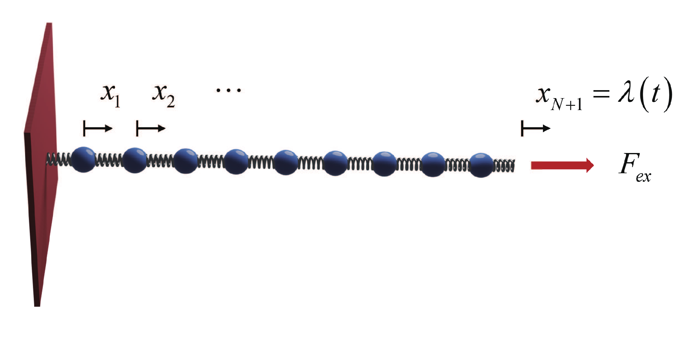
The first example that we examine is a prototype for polymers [32], and biological macromolecules such as DNA and coiled-coil proteins [26]. In particular, the model consists of N𝑁N particles following Langevin dynamics, connected through N+1𝑁1N+1 identical springs, as shown in Fig. 3. The first spring is fixed to a wall, while the last one has a prescribed displacement boundary condition of the form xN+1=λ(t)=vptsubscript𝑥𝑁1𝜆𝑡subscript𝑣𝑝𝑡x_{N+1}=\lambda(t)=v_{p}t, where vpsubscript𝑣𝑝v_{p} is a constant pulling velocity. Denoting by V~ssubscript~𝑉𝑠\tilde{V}_{s} the potential energy of an individual spring for the system being simulated (system S~~𝑆\tilde{S}), the governing equations read

{ηx˙i=V~s(xi+1xi)V~s(xixi1)+σξ˙i,i=1,2,,N1ηx˙N=V~s(λ(t)xN)V~s(xNxN1)+σξ˙N.,\left\{\begin{aligned} &\eta\dot{x}_{i}=\tilde{V}^{\prime}_{s}(x_{i+1}-x_{i})-\tilde{V}^{\prime}_{s}(x_{i}-x_{i-1})+\sqrt{\sigma}\dot{\xi}_{i},&&i=1,2,\cdots,N-1\\ &\eta\dot{x}_{N}=\tilde{V}^{\prime}_{s}(\lambda(t)-x_{N})-\tilde{V}^{\prime}_{s}(x_{N}-x_{N-1})+\sqrt{\sigma}\dot{\xi}_{N}.\end{aligned}\right., (30)

where σ=2kbTη𝜎2subscript𝑘𝑏𝑇𝜂\sigma=2k_{b}T\eta.

In the following, we will consider three specific combinations of systems S𝑆S and S~~𝑆\tilde{S} to demonstrate the versatility of the approach and the quality of the UQ estimates. These include

  1. \bullet

    Element transmutation. In this first example, we will aim at predicting the behavior of material S𝑆S from S~~𝑆\tilde{S} (different potential energies), while subjected to the same pulling protocol. This is similar to the implementation of hyperdynamics [1] or path reweighting method [3], where the potential is the only varying parameter between the simulated and the predicted system.

  2. \bullet

    Predicting the far-from-equilibrium response of a material from its equilibrium behavior. Here, the potential energy will remain the same, while the pulling velocity will change from 0 (equilibrium) to a finite value (away from equilibrium).

  3. \bullet

    For the last example, we will change both the potential energy and the pulling protocol. In particular, we will consider the extreme case of predicting the non-equilibrium response of a nonlinear interacting mass-spring chain from independent Brownian particles, i.e., V~=0~𝑉0\tilde{V}=0.

In each of these cases, we will consider observables that widely range in nature: from the expected evolution of each particle, to the instantaneous force exerted on the system at a given time, to the work done over a given time interval, which of course depends on the full evolution. For all cases, we choose N=10𝑁10N=10 particles, temperature kBT=104subscript𝑘𝐵𝑇superscript104k_{B}T=10^{-4}, viscosity η=5𝜂5\eta=5, interparticle potentials Vssubscript𝑉𝑠V_{s} and V~ssubscript~𝑉𝑠\tilde{V}_{s} of quartic form, i.e., 12k2x2+14k4x412subscript𝑘2superscript𝑥214subscript𝑘4superscript𝑥4\frac{1}{2}k_{2}x^{2}+\frac{1}{4}k_{4}x^{4}, and we will perform NR=105subscript𝑁𝑅superscript105N_{R}=10^{5} realizations of system S~~𝑆\tilde{S}. The Langevin equations will be numerically simulated using an Euler-Maruyama scheme [30] with a time step Δt=103Δ𝑡superscript103\Delta t=10^{-3}. For comparison purposes, material/process S𝑆S will also be simulated, and the same number of realizations will be used to directly estimate the ensemble averages.

For the uncertainty quantification estimates, we choose the reference trajectory 𝐱r(t)=𝟎subscript𝐱𝑟𝑡0\mathbf{x}_{r}(t)=\mathbf{0} and use 100 time steps in the discretization for each evaluated time point. That is, for each time at which the variance of 𝒫biassubscript𝒫𝑏𝑖𝑎𝑠\mathcal{P}_{bias} is computed, a value of nT=100subscript𝑛𝑇100n_{T}=100 is chosen in the calculation of the coefficients 𝐀sqsubscript𝐀𝑠𝑞\mathbf{A}_{sq}, 𝐛sqsubscript𝐛𝑠𝑞\mathbf{b}_{sq} and csqsubscript𝑐𝑠𝑞c_{sq}, according to Eqs. (22), (23) and (24), respectively. We remark that although 𝐱r(t)=𝟎subscript𝐱𝑟𝑡0\mathbf{x}_{r}(t)=\mathbf{0} does not correspond in all cases to the expected trajectory of system/process S~~𝑆\tilde{S}, this choice greatly simplifies the calculations and leads to remarkably accurate estimates for σ𝒫bias2subscriptsuperscript𝜎2subscript𝒫𝑏𝑖𝑎𝑠\sigma^{2}_{\mathcal{P}_{bias}} and |𝒩1|𝒩1\left|\mathcal{N}-1\right|.

Refer to caption
Figure 3: Schematics of the 1D mass-spring system used in Example 1. Reprinted from [33] Harnessing fluctuation theorems to discover free energy and dissipation potentials from non-equilibrium data, Vol 145, Shenglin Huang, Chuanpeng Sun, Prashant K. Purohit, Celia Reina, Page 3, Copyright (2021), with permission from Elsevier.

4.2 Case 1: Element transmutation: from material S~~𝑆\tilde{S} to material S𝑆S subjected to the same pulling protocol

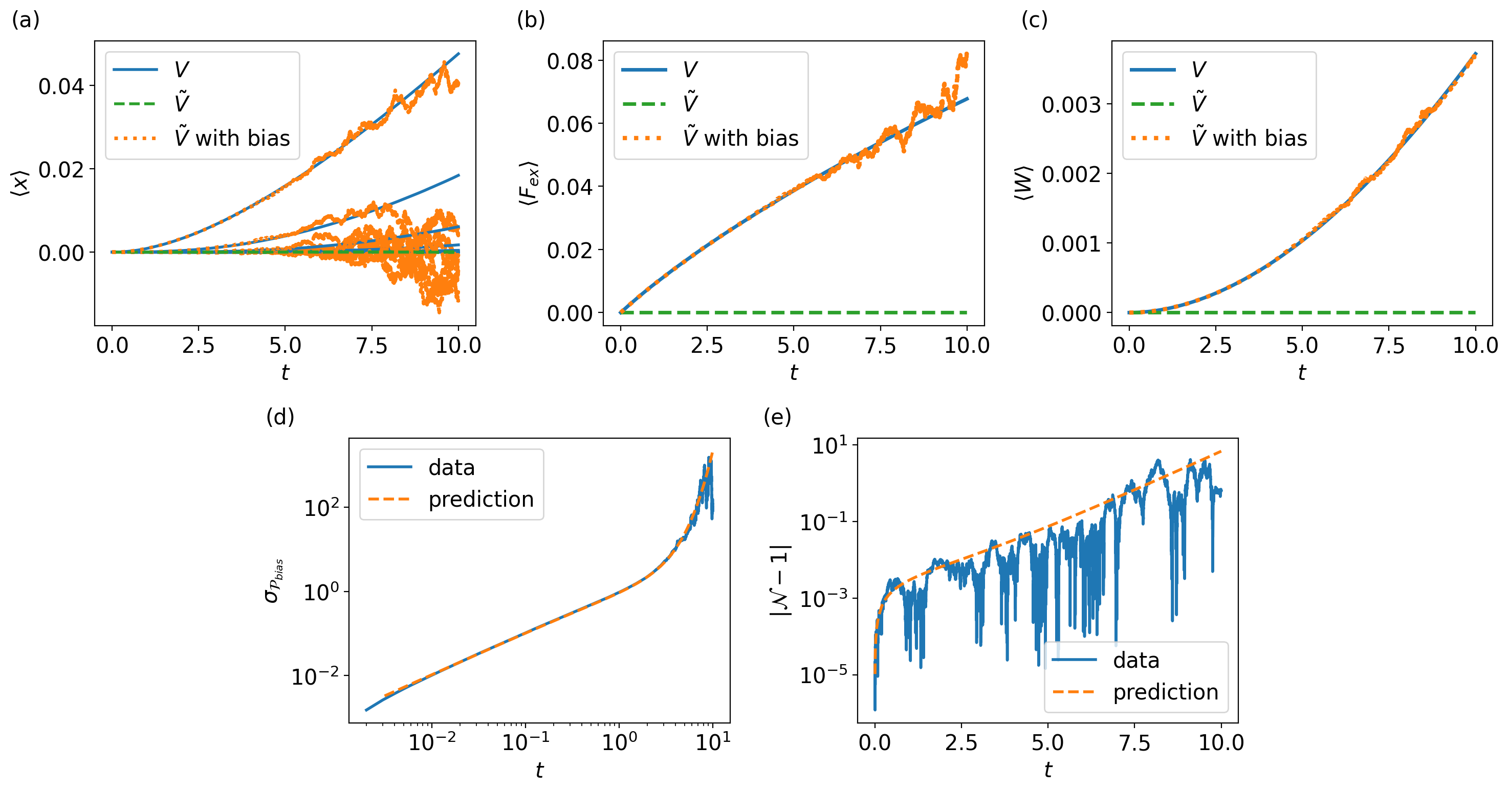
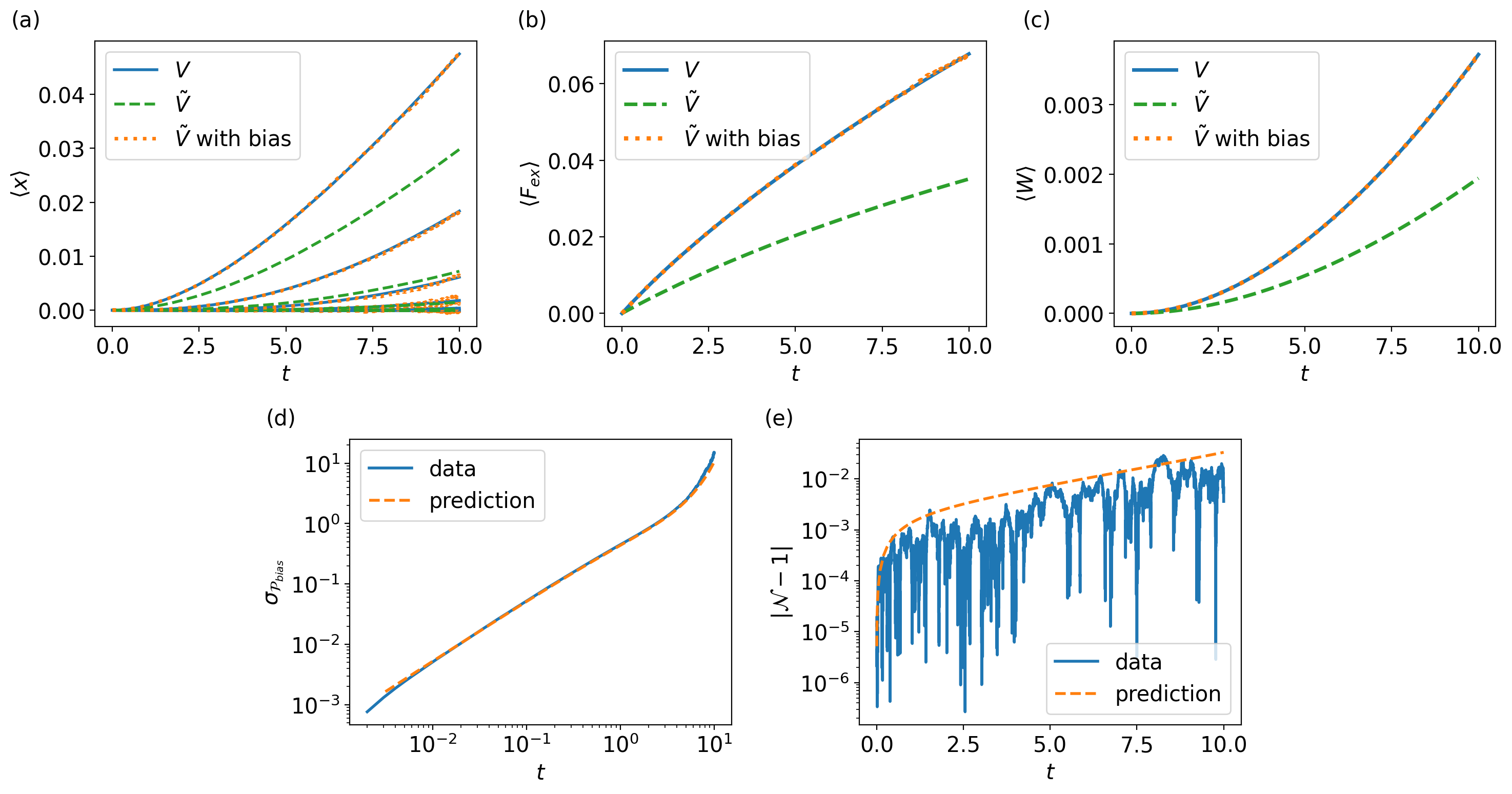
This first case demonstrates the capability of the method for predicting the non-equilibrium response of a system with an anharmonic potential, namely Vs(u)=12k2u2+14k4u4subscript𝑉𝑠𝑢12subscript𝑘2superscript𝑢214subscript𝑘4superscript𝑢4V_{s}(u)=\frac{1}{2}k_{2}u^{2}+\frac{1}{4}k_{4}u^{4} (material S𝑆S) from a harmonic one, V~=12k~2u2~𝑉12subscript~𝑘2superscript𝑢2\tilde{V}=\frac{1}{2}\tilde{k}_{2}u^{2}, (material S~~𝑆\tilde{S}), under the same pulling protocol λ˙(t)=λ~˙(t)=vp˙𝜆𝑡˙~𝜆𝑡subscript𝑣𝑝\dot{\lambda}(t)=\dot{\tilde{\lambda}}(t)=v_{p}. Here, we choose k~2=0.5subscript~𝑘20.5\tilde{k}_{2}=0.5, k2=1subscript𝑘21k_{2}=1, k4=100subscript𝑘4100k_{4}=100 and vp=0.01subscript𝑣𝑝0.01v_{p}=0.01. Figures  4 (a-c) show the results for the ensemble averages of the displacement of each particle xidelimited-⟨⟩subscript𝑥𝑖\left<x_{i}\right>, the external force applied on the system Fexdelimited-⟨⟩subscript𝐹𝑒𝑥\left<F_{ex}\right> and the external work Wdelimited-⟨⟩𝑊\left<W\right>. The blue solid lines, green dashed lines and orange dotted lines represent, respectively, the results from Langevin simulation for system S𝑆S with potential V𝑉V, those for system S~~𝑆\tilde{S} with potential V~~𝑉\tilde{V}, and the prediction of system S𝑆S from S~~𝑆\tilde{S} using Eq. (4). In particular, the lines from bottom to the top in Fig. 4(a) represent the particles from 1 to N=10𝑁10N=10. As it is there observed, all predictions are in excellent agreement with the validation data. Only very minor differences for the average displacement and external force are observed after around t8similar-to𝑡8t\sim 8, where the predictions become slightly more stochastic in nature. These increase in the errors are to be expected as noted at the end of Section 2 and can be predicted using the nonlinear uncertainty quantification estimates discussed in Sec. 3.2. We recall that these estimates aim at predicting the deviation of the empirical average 𝒩=r=1NR1NR𝒫bias,r𝒩superscriptsubscript𝑟1subscript𝑁𝑅1subscript𝑁𝑅subscript𝒫𝑏𝑖𝑎𝑠𝑟\mathcal{N}=\sum_{r=1}^{N_{R}}\frac{1}{N_{R}}\mathcal{P}_{bias,r} from one through σ𝒩=σ𝒫bias/NRsubscript𝜎𝒩subscript𝜎subscript𝒫𝑏𝑖𝑎𝑠subscript𝑁𝑅\sigma_{\mathcal{N}}=\sigma_{\mathcal{P}_{bias}}/\sqrt{N_{R}}, which itself is used as a measure of how well the path probability distribution of the system S𝑆S (the one not simulated) is captured. Figures 4(d, e) show the estimated growing standard deviation of factor 𝒫biassubscript𝒫𝑏𝑖𝑎𝑠\mathcal{P}_{bias} in a log-log scale and the deviation of 𝒩𝒩\mathcal{N} from one in a log-linear scale, respectively, compared to the corresponding values directly calculated from the Langevin simulation. Remarkably, without simulation data for neither system S𝑆S nor system S~~𝑆\tilde{S}, the derived estimates perfectly predict the standard deviation of 𝒫biassubscript𝒫𝑏𝑖𝑎𝑠\mathcal{P}_{bias}, which spans four decades, and the deviation of 𝒩𝒩\mathcal{N}. As time increase, the deviation of 𝒩𝒩\mathcal{N} finally reaches 3%percent33\%, which is tolerable and agrees well with the small errors in the observables. We note that the accuracy of these results is striking, as the bias potential is not purely quadratic (for which the estimates would be exact), but instead include a non-negligible quartic contribution.
Refer to caption
Figure 4: Prediction of the non-equilibrium behavior of material S𝑆S with quartic interatomic potential Vs(u)=12k2u2+14k4u4subscript𝑉𝑠𝑢12subscript𝑘2superscript𝑢214subscript𝑘4superscript𝑢4V_{s}(u)=\frac{1}{2}k_{2}u^{2}+\frac{1}{4}k_{4}u^{4} from material S~~𝑆\tilde{S} with quadratic potential V~s(u)=12k~2u2subscript~𝑉𝑠𝑢12subscript~𝑘2superscript𝑢2\tilde{V}_{s}(u)=\frac{1}{2}\tilde{k}_{2}u^{2} under the same pulling velocity λ˙(t)=λ~˙(t)=vp(t)˙𝜆𝑡˙~𝜆𝑡subscript𝑣𝑝𝑡\dot{\lambda}(t)=\dot{\tilde{\lambda}}(t)=v_{p}(t), where k~2=0.5subscript~𝑘20.5\tilde{k}_{2}=0.5, k2=1subscript𝑘21k_{2}=1, k4=100subscript𝑘4100k_{4}=100 and vp(t)=0.01subscript𝑣𝑝𝑡0.01v_{p}(t)=0.01. (a-c) Results for the ensemble averages of three different observables: (a) the displacement of each particle xidelimited-⟨⟩subscript𝑥𝑖\left<x_{i}\right>, with i=1,,10𝑖110i=1,\dots,10 from bottom to top, (b) the external force Fexdelimited-⟨⟩subscript𝐹𝑒𝑥\left<F_{ex}\right> and (c) the external work Wdelimited-⟨⟩𝑊\left<W\right>. The blue solid lines and green dashed lines are the results from Langevin simulation for material S𝑆S and S~~𝑆\tilde{S}, respectively. The orange dotted lines are the predictions for material S𝑆S from material S~~𝑆\tilde{S}. (d, e) Validation of the uncertainty quantification estimates by evaluating the time evolution of (d) the standard deviation of 𝒫biassubscript𝒫𝑏𝑖𝑎𝑠\mathcal{P}_{bias} and (e) the deviation of the empirical factor 𝒩𝒩\mathcal{N} from one. The solid blue lines are the exact value from the data and the orange dotted lines are the predictions using the nonlinear uncertainty quantification method.

4.3 Case 2: From equilibrium to non-equilibrium for the same material

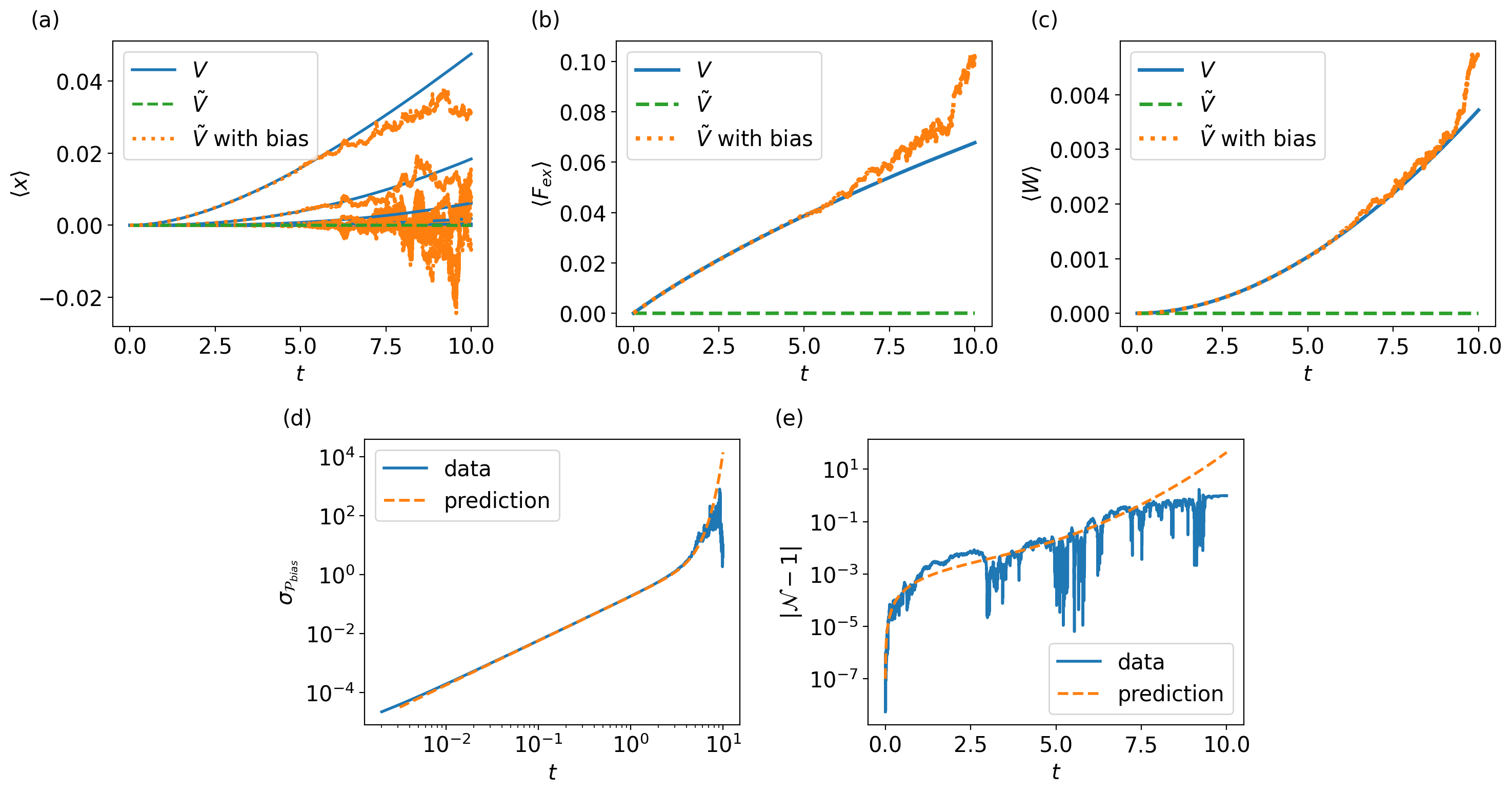
In contrast to the first case, this second case illustrates the prediction of the non-equilibrium response for a given system (finite pulling velocity) given its equilibrium behavior (zero pulling velocity). The interatomic potential considered is Vs(u)=V~s(u)=12k2u2+14k4u4subscript𝑉𝑠𝑢subscript~𝑉𝑠𝑢12subscript𝑘2superscript𝑢214subscript𝑘4superscript𝑢4V_{s}(u)=\tilde{V}_{s}(u)=\frac{1}{2}k_{2}u^{2}+\frac{1}{4}k_{4}u^{4}, with k2=1subscript𝑘21k_{2}=1 and k4=100subscript𝑘4100k_{4}=100, and the pulling velocity for the aimed non-equilibrium process is λ˙(t)=vp=0.01˙𝜆𝑡subscript𝑣𝑝0.01\dot{\lambda}(t)=v_{p}=0.01. Figures 5(a-c) depict the prediction for the average displacement of each particle, average external force and average work. While all the predictions have good agreements with the true results at the beginning, the errors start to become more significant from about t6similar-to𝑡6t\sim 6, at which point the ensemble averages appear to be more stochastic in nature. This increased stochasticity results from a decrease in the number of trajectories that contribute in practice to the ensemble average and is directly related to the heavier tails of 𝒫biassubscript𝒫𝑏𝑖𝑎𝑠\mathcal{P}_{bias} discussed in Section 2. The larger errors, as compared to Case 1 studied in Section 4.2, are also understandable from a sampling perspective. In the process to be predicted, all the particles (especially the last few ones) are moving rightward in the most probable trajectories induced by the positive pulling velocity. However, these trajectories are highly unlikely to be observed at equilibrium, where the right end is fixed. Hence, the predicted evolution of the observables (especially the average displacement for the last particle and, consequently, the average external force and work) are biased. Figures 5(d, e) show the growing standard deviation of factor 𝒫biassubscript𝒫𝑏𝑖𝑎𝑠\mathcal{P}_{bias} and the deviation of the normalization factor 𝒩𝒩\mathcal{N} from one. The latter reaches an error of 0.1 at around t8similar-to𝑡8t\sim 8, at which time the prediction for the observables becomes very poor and are no longer reliable. Here, again, the uncertainty quantification estimates provide an excellent prediction of the sampling errors.
Refer to caption
Figure 5: Predicton of the non-equilibrium behavior under pulling velocity λ˙(t)=vp(t)>0˙𝜆𝑡subscript𝑣𝑝𝑡0\dot{\lambda}(t)=v_{p}(t)>0 (process S𝑆S) from the equilibrium response, i.e., λ~˙(t)=0˙~𝜆𝑡0\dot{\tilde{\lambda}}(t)=0, (process S~~𝑆\tilde{S}) for the same material with quartic interatomic potential Vs(u)=V~s(u)=12k2u2+14k4u4subscript𝑉𝑠𝑢subscript~𝑉𝑠𝑢12subscript𝑘2superscript𝑢214subscript𝑘4superscript𝑢4V_{s}(u)=\tilde{V}_{s}(u)=\frac{1}{2}k_{2}u^{2}+\frac{1}{4}k_{4}u^{4}, where k2=1subscript𝑘21k_{2}=1, k4=100subscript𝑘4100k_{4}=100 and vp(t)=0.01subscript𝑣𝑝𝑡0.01v_{p}(t)=0.01. (a-c) Results for the ensemble averages of three different observables: (a) the displacement of each particle xidelimited-⟨⟩subscript𝑥𝑖\left<x_{i}\right>, (b) the external force Fexdelimited-⟨⟩subscript𝐹𝑒𝑥\left<F_{ex}\right> and (c) the external work Wdelimited-⟨⟩𝑊\left<W\right>. The blue solid lines and green dashed lines are the results from Langevin simulation with process S𝑆S and process S~~𝑆\tilde{S}, respectively. The orange dotted lines are the prediction for process S𝑆S from process S~~𝑆\tilde{S}. (d, e) Validation of the uncertainty quantification estimates by evaluating the time evolution of (d) the standard deviation of Pbiassubscript𝑃𝑏𝑖𝑎𝑠P_{bias} and (e) the deviation of the empirical factor 𝒩𝒩\mathcal{N} from one. The solid blue lines are the exact value from the data and the orange dotted lines are the predictions using the nonlinear uncertainty quantification method.

4.4 Case 3: From Brownian particles to the non-equilibrium response of an interacting particle system

The third and final case considered is aimed at demonstrating an extreme example for the path reweighting strategy. Specifically, we choose to predict the non-equilibrium behavior of an anharmonic chain from independent Brownian particles, i.e., V~=0~𝑉0\tilde{V}=0. Here, material/process S𝑆S is also set as a quartic interatomic potential Vs(u)=12k2u2+14k4u4subscript𝑉𝑠𝑢12subscript𝑘2superscript𝑢214subscript𝑘4superscript𝑢4V_{s}(u)=\frac{1}{2}k_{2}u^{2}+\frac{1}{4}k_{4}u^{4} with k2=1subscript𝑘21k_{2}=1 and k4=100subscript𝑘4100k_{4}=100 with pulling velocity λ˙(t)=vp=0.01˙𝜆𝑡subscript𝑣𝑝0.01\dot{\lambda}(t)=v_{p}=0.01. Figures 6(a-c) depict the predictions for the average displacement, average external force and average work. Despite the extreme nature of the example, the predictions are still reasonably good up to t=10𝑡10t=10, and actually better than that of Case 2 above. Here, the Brownian particles can freely move, while those of Case 2 are constrained due to the boundary conditions and interatomic potential for system S~~𝑆\tilde{S}. This significantly reduces the sampling errors that govern the accuracy of the predictions. Finally, Figures 6(d, e) show the growing standard deviation of 𝒫biassubscript𝒫𝑏𝑖𝑎𝑠\mathcal{P}_{bias} with time and the deviation of 𝒩𝒩\mathcal{N} with one. Again, the UQ estimates perfectly predict both quantities throughout six decades. Moreover, the error of |𝒩1|𝒩1|\mathcal{N}-1| reaches 10%percent1010\% around t6similar-to𝑡6t\sim 6, after which the number of realizations of system S~~𝑆\tilde{S} is insufficient to accurately make predictions of system S𝑆S.

Refer to caption
Figure 6: Prediction of the non-equilibrium behavior for material S𝑆S with quartic interatomic potential Vs(u)=12k2u2+14k4u4subscript𝑉𝑠𝑢12subscript𝑘2superscript𝑢214subscript𝑘4superscript𝑢4V_{s}(u)=\frac{1}{2}k_{2}u^{2}+\frac{1}{4}k_{4}u^{4}, with k2=1subscript𝑘21k_{2}=1, k4=100subscript𝑘4100k_{4}=100, under pulling velocity λ˙(t)=vp(t)=0.01˙𝜆𝑡subscript𝑣𝑝𝑡0.01\dot{\lambda}(t)=v_{p}(t)=0.01 from Brownian trajectories. (a-c) Results for the ensemble averages of three different observables: (a) the displacement of each particle xidelimited-⟨⟩subscript𝑥𝑖\left<x_{i}\right>, (b) the external force Fexdelimited-⟨⟩subscript𝐹𝑒𝑥\left<F_{ex}\right> and (c) the external work Wdelimited-⟨⟩𝑊\left<W\right>. The blue solid lines and green dashed lines are the results from Langevin simulations of system/process S𝑆S and S~~𝑆\tilde{S}, respectively. The orange dotted lines are the prediction for material/process S𝑆S from S~~𝑆\tilde{S}. (d, e) Validation of the uncertainty quantification estimates by evaluating the time evolution of (d) the standard deviation of Pbiassubscript𝑃𝑏𝑖𝑎𝑠P_{bias} and (e) the deviation of the empirical factor 𝒩𝒩\mathcal{N} from one. The solid blue lines are the exact value from the data and the orange dotted lines are the predictions using the nonlinear uncertainty quantification method.

5 Example 2: Caging in two-dimensional glassy systems

One of the most ubiquitous examples of out-of-equilibrium behavior, and one that we are regularly familiar with from everyday experience, is that of glasses [34, 35]. Glassy dynamics is observed in a wide range of length scales (from nanoparticles to grains) spanning a variety of industries from building materials (concrete) to paints (colloidal suspensions), and household goods (foams & gels)[36, 37]. Despite the ubiquity of glassy systems, the study of equilibrium statistical mechanics leaves us ill-equipped to answer many questions surrounding the theory of glasses, though there has been significant recent progress [38]. In these final examples, we aim to predict features of the glassy dynamics from the motions of particles in the equilibrium, fluid phase of 2D glass-formers. Supercooled liquids above their glass transition temperature exhibit a characteristic onset of “caged” dynamics, whereby particles vibrate in the cage formed by their neighbors before thermal fluctuations enable hopping past the cage. This phenomenon of particle localization is usually called caging, and can be observed in many dynamical quantities. The mean squared displacement (𝒮𝒟𝒮𝒟\mathcal{MSD}), familiar to many from the study of Brownian motion, is sufficient to explain such behavior. The emergence of sub-diffusive (slope << 1) trends in the log-log fits to 𝒮𝒟𝒮𝒟\mathcal{MSD} is a hallmark of the onset of particle caging, where as the observance of a plateau is indicative of strongly caged dynamics, and the duration of the cage grows at the materials cooled towards the glass transition.

5.1 Model description and overview of the cases to be examined

Here, we explore two model systems, a bidisperse mixture of Hertzian disks and the standard Kob-Anderson type Lennard-Jones glass, shown in Fig. 7. The Hertzian system is defined by an interparticle potential

Vij(r)={0.4ϵ(1rσij)2.5rσij0r>σijsubscript𝑉𝑖𝑗𝑟cases0.4italic-ϵsuperscript1𝑟subscript𝜎𝑖𝑗2.5𝑟subscript𝜎𝑖𝑗0𝑟subscript𝜎𝑖𝑗V_{ij}(r)=\begin{cases}0.4\epsilon\left(1-\frac{r}{\sigma_{ij}}\right)^{2.5}&r\leq\sigma_{ij}\\ 0&r>\sigma_{ij}\end{cases} (31)

with a 50:50 A:B mixture, where σAB=1.2σAAsubscript𝜎𝐴𝐵1.2subscript𝜎𝐴𝐴\sigma_{AB}=1.2\sigma_{AA} and σBB=1.4σAAsubscript𝜎𝐵𝐵1.4subscript𝜎𝐴𝐴\sigma_{BB}=1.4\sigma_{AA}. A constant packing fraction of 1.0σAA2subscriptsuperscript𝜎2𝐴𝐴\sigma^{-2}_{AA} is used. The Lennard-Jones system uses the usual interparticle potential with a numerical cut-off distance

Vij(r)={4ϵij[(σijr)12(σijr)6]r2.5σij0r>2.5σijsubscript𝑉𝑖𝑗𝑟cases4subscriptitalic-ϵ𝑖𝑗delimited-[]superscriptsubscript𝜎𝑖𝑗𝑟12superscriptsubscript𝜎𝑖𝑗𝑟6𝑟2.5subscript𝜎𝑖𝑗0𝑟2.5subscript𝜎𝑖𝑗V_{ij}(r)=\begin{cases}4\epsilon_{ij}\left[\left(\frac{\sigma_{ij}}{r}\right)^{12}-\left(\frac{\sigma_{ij}}{r}\right)^{6}\right]&r\leq 2.5\sigma_{ij}\\ 0&r>2.5\sigma_{ij}\end{cases} (32)

in a 60:40 A:B mixture, where the interaction lengths are set to σAB=0.8σAAsubscript𝜎𝐴𝐵0.8subscript𝜎𝐴𝐴\sigma_{AB}=0.8\sigma_{AA} and σBB=0.88σAAsubscript𝜎𝐵𝐵0.88subscript𝜎𝐴𝐴\sigma_{BB}=0.88\sigma_{AA}, the energies are set to ϵAB=1.5ϵAAsubscriptitalic-ϵ𝐴𝐵1.5subscriptitalic-ϵ𝐴𝐴\epsilon_{AB}=1.5\epsilon_{AA} and ϵBB=0.5ϵAAsubscriptitalic-ϵ𝐵𝐵0.5subscriptitalic-ϵ𝐴𝐴\epsilon_{BB}=0.5\epsilon_{AA}, and a packing fraction of 1.1σAA2subscriptsuperscript𝜎2𝐴𝐴\sigma^{-2}_{AA} is selected. We choose this species ratio and packing fraction to reduce the chance of crystallization within the system, as the usual 80:20 mixture used in 3D is more prone to do so in 2D [39, 40]. Both systems are composed of 10 particles and σAAsubscript𝜎𝐴𝐴\sigma_{AA} is taken to be 1 universally. Additionally, the simulations are performed in a square, periodic box, and no external forcing is applied to the configurations. As above, the Euler-Mayurama method [30] is used to integrate the overdamped Langevin dynamics of the system with parameters η=5𝜂5\eta=5, and Δt=103Δ𝑡superscript103\Delta t=10^{-3}. We compare our results among two different temperatures kBT{101,102}subscript𝑘𝐵𝑇superscript101superscript102k_{B}T\in\{10^{-1},10^{-2}\}. In the unbiased simulations, we choose pairings of ϵ~~italic-ϵ\tilde{\epsilon} and kBTsubscript𝑘𝐵𝑇k_{B}T such that we observe phenomenology consistent with dynamical arrest if we were to increase ϵ~~italic-ϵ\tilde{\epsilon} or decrease kBTsubscript𝑘𝐵𝑇k_{B}T. Thus, we use ϵ~=10.0~italic-ϵ10.0\tilde{\epsilon}=10.0 when kBT=101subscript𝑘𝐵𝑇superscript101k_{B}T=10^{-1} and ϵ~=1.0~italic-ϵ1.0\tilde{\epsilon}=1.0 when kBT=102subscript𝑘𝐵𝑇superscript102k_{B}T=10^{-2} in the Hertzian case, and ϵ~AA=0.1subscript~italic-ϵ𝐴𝐴0.1\tilde{\epsilon}_{AA}=0.1 when kBT=101subscript𝑘𝐵𝑇superscript101k_{B}T=10^{-1} and ϵ~AA=0.01subscript~italic-ϵ𝐴𝐴0.01\tilde{\epsilon}_{AA}=0.01 when kBT=102subscript𝑘𝐵𝑇superscript102k_{B}T=10^{-2} in the Lennard-Jones model. A total of NR=107subscript𝑁𝑅superscript107N_{R}=10^{7} realizations of the liquid phase in each system were simulated to perform predictions, and another NR=105subscript𝑁𝑅superscript105N_{R}=10^{5} are produced to validate the accuracy of these results.
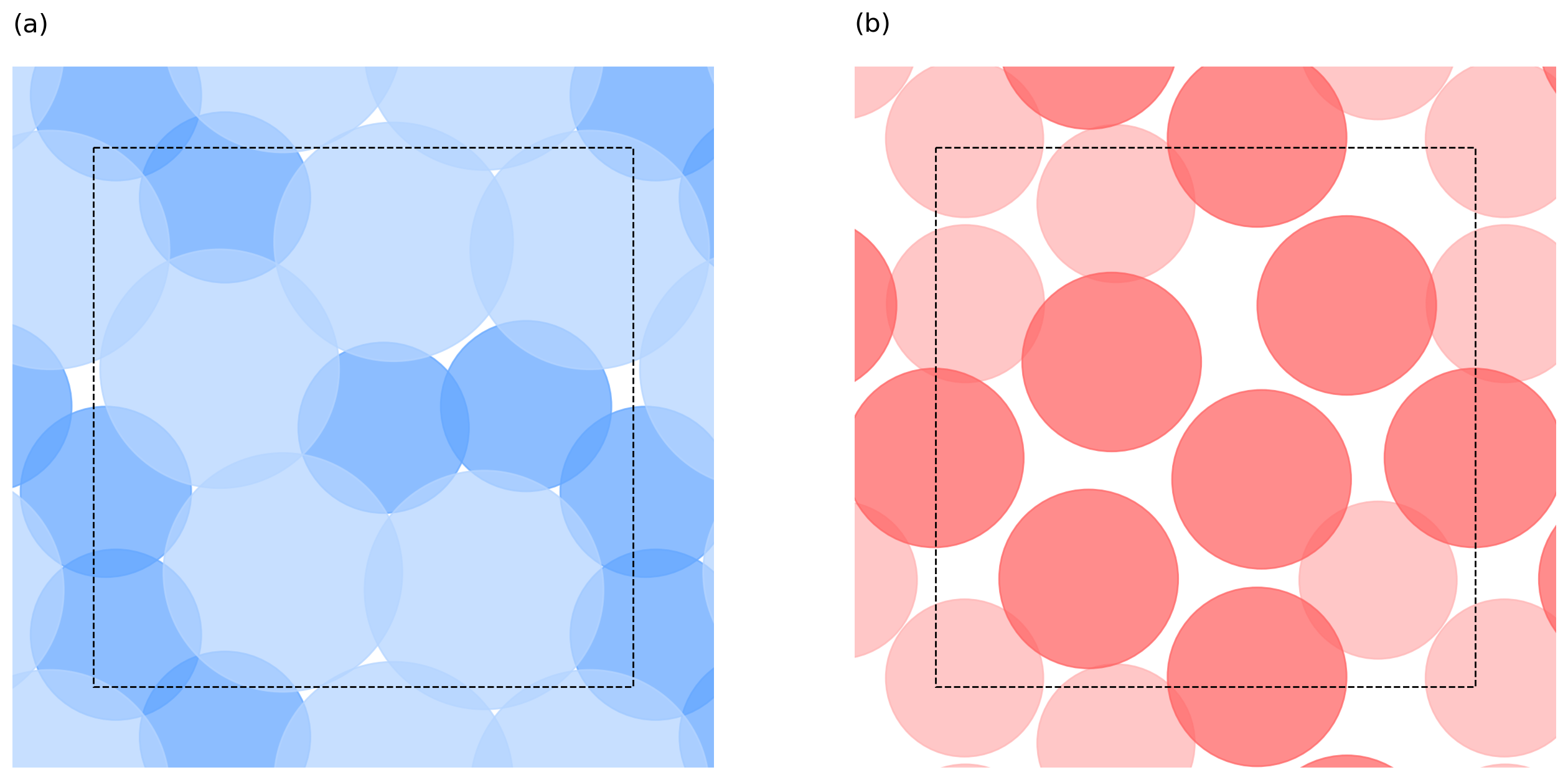
Refer to caption
Figure 7: Initial configurations used in Example 2. (a) Hertzian system in a 50:50 mixture. Dark blue particles are A type and light blue are B type. (b) Lennard-Jones system in a 60:40 mixture. Dark red are A type and light red are B type. The radii of the particles reflect a size of 0.5σiisubscript𝜎𝑖𝑖\sigma_{ii} for particle species i𝑖i. The black dashed square is the boundary of the simulation box.

To analyze the results of our simulations we compute two dynamical quantities, the mean squared displacement 𝒮𝒟𝒮𝒟\mathcal{MSD} and the particle overlap Q(a)𝑄𝑎Q(a), defined as

𝒮𝒟=1Ni=1NΔ𝐫i2,𝒮𝒟delimited-⟨⟩1𝑁superscriptsubscript𝑖1𝑁superscriptnormΔsubscript𝐫𝑖2\displaystyle\mathcal{MSD}=\left\langle\frac{1}{N}\sum_{i=1}^{N}\|\Delta\mathbf{r}_{i}\|^{2}\right\rangle, (33)
Q(a)=1Ni=1NH(aΔ𝐫i),𝑄𝑎delimited-⟨⟩1𝑁superscriptsubscript𝑖1𝑁𝐻𝑎normΔsubscript𝐫𝑖\displaystyle Q(a)=\left\langle\frac{1}{N}\sum_{i=1}^{N}H(a-\|\Delta\mathbf{r}_{i}\|)\right\rangle, (34)

where H𝐻H is the Heaviside step function. The overlap Q(a)𝑄𝑎Q(a) quantifies the fraction of particles that have moved some distance a𝑎a within the simulation box. The overlap function in this context conveys essentially the same information as the self-intermediate scattering function, also commonly used in the glassy literature. We choose a=0.1𝑎0.1a=0.1 in all simulations to display the onset of caged dynamics at accessible timescales.

While the glass transition can normally be observed by lowering the system temperature until plateaus are viewed in quantities like the 𝒮𝒟𝒮𝒟\mathcal{MSD} and Q(a)𝑄𝑎Q(a), we here vary instead the energy scale ϵitalic-ϵ\epsilon relative to kBTsubscript𝑘𝐵𝑇k_{B}T to increase the height of energetic barriers and induce caging. We prepare the initial state of each system to be completely force balanced, thus making the initial dynamics nearly degenerate regarding the energy scale ϵitalic-ϵ\epsilon. Initially, states are sampled from a spatially uniform distribution and the configurations are subsequently quenched to their inherent structure using gradient descent [41]. In each system, we only employ one initial configuration, where we observe phenomenology consistent with caged dynamics to generate our realizations.

Since we only modify the potential through a scaling coefficient between our reference and target systems, we can pull the difference in V~~𝑉\tilde{V} and V𝑉V through the integration. This leaves us with two terms in the computation of biassubscript𝑏𝑖𝑎𝑠\mathcal{I}_{bias}, denoted below as 1subscript1\mathcal{I}_{1} and 2subscript2\mathcal{I}_{2}

Vbias𝐫i=(1ϵϵ~)V~𝐫i=(χ1)V~𝐫i,subscript𝑉𝑏𝑖𝑎𝑠subscript𝐫𝑖1italic-ϵ~italic-ϵ~𝑉subscript𝐫𝑖𝜒1~𝑉subscript𝐫𝑖\frac{\partial V_{bias}}{\partial\mathbf{r}_{i}}=\left(1-\frac{\epsilon}{\tilde{\epsilon}}\right)\frac{\partial\tilde{V}}{\partial\mathbf{r}_{i}}=-\left(\chi-1\right)\frac{\partial\tilde{V}}{\partial\mathbf{r}_{i}}, (35)
bias=(χ1)24η0τiNV~𝐫i2dt+(χ1)kBT2η0τiNV~𝐫i𝝃˙idt=2(χ1)21(χ1).subscript𝑏𝑖𝑎𝑠superscript𝜒124𝜂superscriptsubscript0𝜏superscriptsubscript𝑖𝑁superscriptdelimited-∥∥~𝑉subscript𝐫𝑖2𝑑𝑡𝜒1subscript𝑘𝐵𝑇2𝜂superscriptsubscript0𝜏superscriptsubscript𝑖𝑁~𝑉subscript𝐫𝑖subscript˙𝝃𝑖𝑑𝑡subscript2superscript𝜒12subscript1𝜒1\begin{split}&\mathcal{I}_{bias}=\frac{(\chi-1)^{2}}{4\eta}\int_{0}^{\tau}\sum_{i}^{N}\left\|\frac{\partial\tilde{V}}{\partial\mathbf{r}_{i}}\right\|^{2}\,dt+(\chi-1)\sqrt{\frac{k_{B}T}{2\eta}}\int_{0}^{\tau}\sum_{i}^{N}\frac{\partial\tilde{V}}{\partial\mathbf{r}_{i}}\cdot\dot{\bm{\xi}}_{i}\,dt=\mathcal{I}_{2}(\chi-1)^{2}-\mathcal{I}_{1}(\chi-1).\end{split} (36)

With this equation in hand, we can compute any member of this family of potentials at virtually no added computational cost; we simply compute the forces for V~~𝑉\tilde{V} once, and then apply Eq. (36) for each desired V𝑉V. In our results, we employ this method to generate predictions at 10 different target potentials with ratios V/V~=χ𝑉~𝑉𝜒V/\tilde{V}=\chi sampled logarithmically from 1.259 to 10.0.
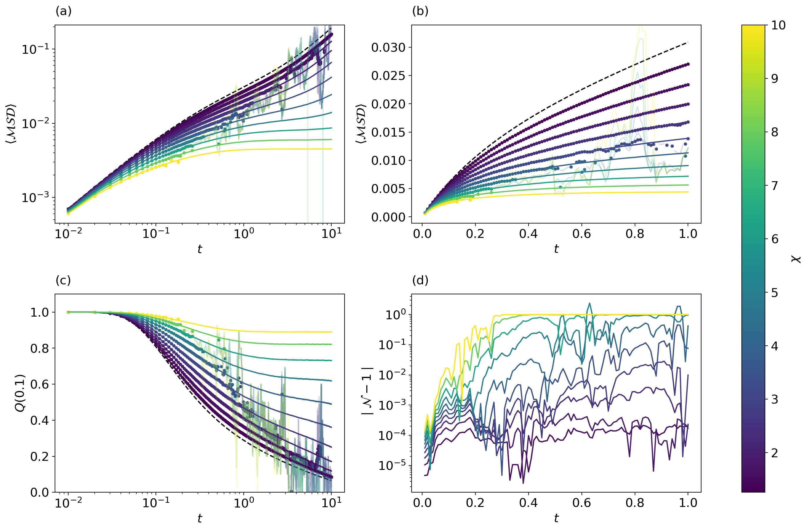
Refer to caption
Figure 8: Observables for the Hertzian case with kBT=101subscript𝑘𝐵𝑇superscript101k_{B}T=10^{-1}, highlighting the transition to caging. Mean squared displacement (a,b) and particle overlap (c) calculated from V~~𝑉\tilde{V} (black dashed line) and validation datasets (bold lines). Prediction points in which |𝒩1|<0.1𝒩10.1|\mathcal{N}-1|<0.1 are plotted with solid dots, otherwise they are plotted with faint lines to highlight the prediction’s deviation from validation. (d) Deviation in 𝒩𝒩\mathcal{N} from unity, indicating when we can be confident in the accuracy of the predicted observables.

5.2 Results

First, we look at both systems with kBT=101subscript𝑘𝐵𝑇superscript101k_{B}T=10^{-1}. In the Hertzian case, shown in Fig. 8, we find good agreement between our prediction and the validation data over a wide range of times. In biases as high as χ=10.0𝜒10.0\chi=10.0, the curves track well, and we can observe dramatically slower dynamics as indicated by the slopes of 𝒮𝒟𝒮𝒟\mathcal{MSD} in Figure 8(a,b). From Figure 8(a) we can see in our simulation of V~~𝑉\tilde{V} (black dashed line) initially diffusive behavior until t0.2similar-to𝑡0.2t\sim 0.2, followed by a period of slight sub-diffusivity, and the reemergence of diffusive behavior after t3.0similar-to𝑡3.0t\sim 3.0. As we increase χ𝜒\chi, the dynamics become more sluggish until we observe a prolonged plateau for χ>5.0𝜒5.0\chi>5.0. We find the same signatures of caged dynamics in Q(0.1)𝑄0.1Q(0.1) shown in Figure 8(c). The length of time before the accuracy of the method breaks down is strongly dependent upon the value of χ𝜒\chi used, where a χ𝜒\chi of 10.0 breaks down at t0.2similar-to𝑡0.2t\sim 0.2, while χ=1.259𝜒1.259\chi=1.259 is accurate well beyond t=10.0𝑡10.0t=10.0. While the caging plateau seen beyond χ5.0similar-to𝜒5.0\chi\sim 5.0 appears to be just out of reach, the sub-diffusive behavior that we can predict is still strong evidence for predicting the onset of caged dynamics from diffusive dynamics.
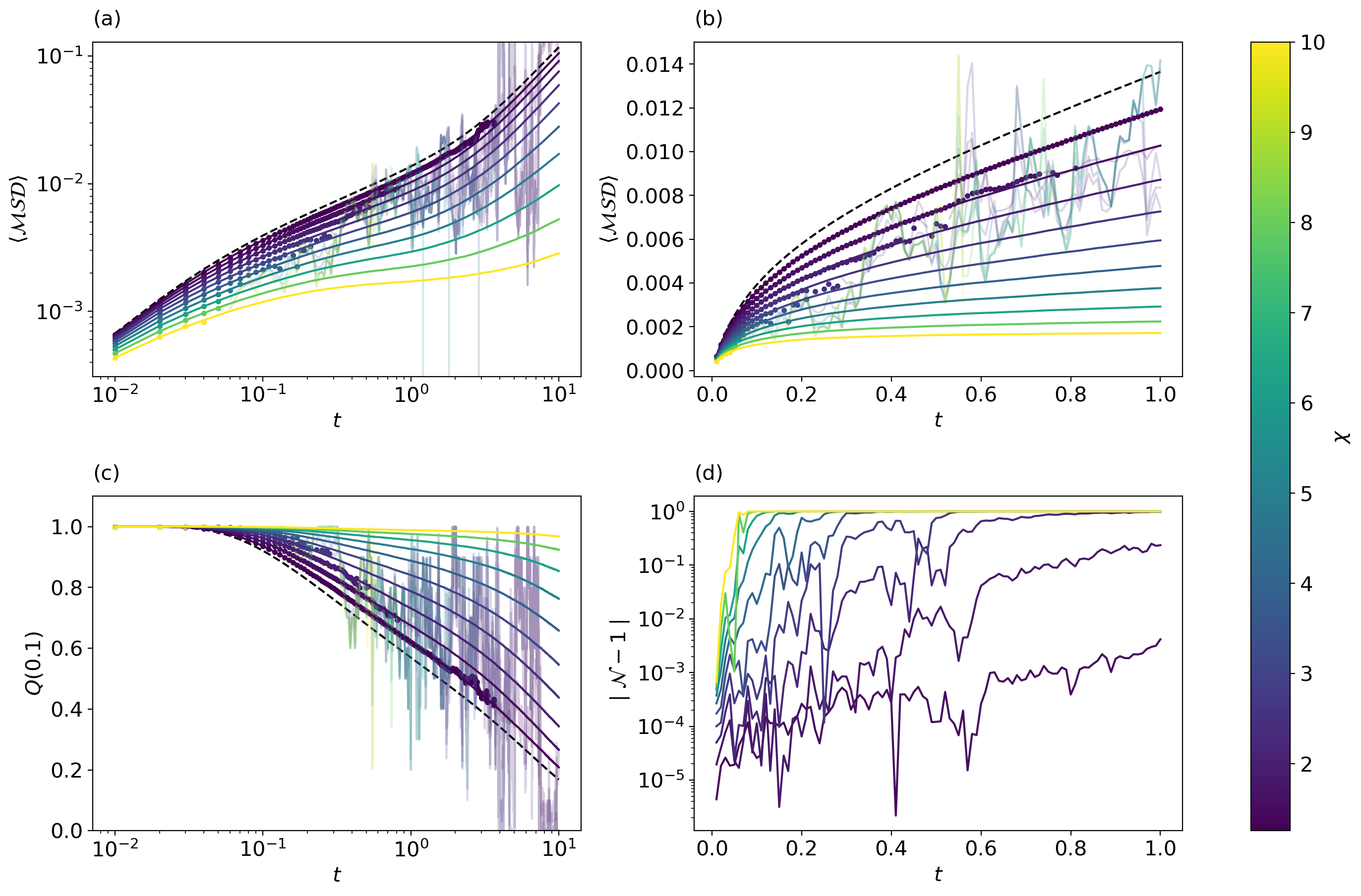
Refer to caption
Figure 9: Observables for the Lennard-Jones case with kBT=101subscript𝑘𝐵𝑇superscript101k_{B}T=10^{-1}, highlighting the transition to caging. Mean squared displacement (a,b) and particle overlap (c) calculated from V~~𝑉\tilde{V} (black dashed line) and validation datasets (bold lines). Prediction points in which |𝒩1|<0.1𝒩10.1|\mathcal{N}-1|<0.1 are plotted with solid dots, otherwise they are plotted with faint lines to highlight the prediction’s deviation from validation. (d) Deviation in 𝒩𝒩\mathcal{N} from unity, indicating when we can be confident in the accuracy of the predicted observables.

Similar tends are seen in the data from the Lennard-Jones model, shown in Figure 9. We find that the predictions break down at shorter times than seen in the Hertzian case. This is likely due to the more rapid emergence of large forces in the Lennard-Jones model compared to the Hertzian system when deviating from the minima of the potential. To further explore this relationship between the potentials, dynamics, and confidence in our predictions, we compute the instantaneous diffusion coefficients D𝐷D from our 𝒮𝒟𝒮𝒟\mathcal{MSD} curves using a simple forward difference method. In Figure 10 we see that the softer repulsion of the Hertzian model leads to a gradual reduction of the diffusion coefficient as the configurations escape the minima, but we find this drop in D𝐷D to happen more rapidly in the Lennard-Jones model. Surprisingly, we find that the breakdown of our prediction appears to occur universally when D𝐷D drops below 0.003similar-toabsent0.003\sim 0.003. This cutoff appears to be set by both the number of realizations and the temperature used for our simulation.
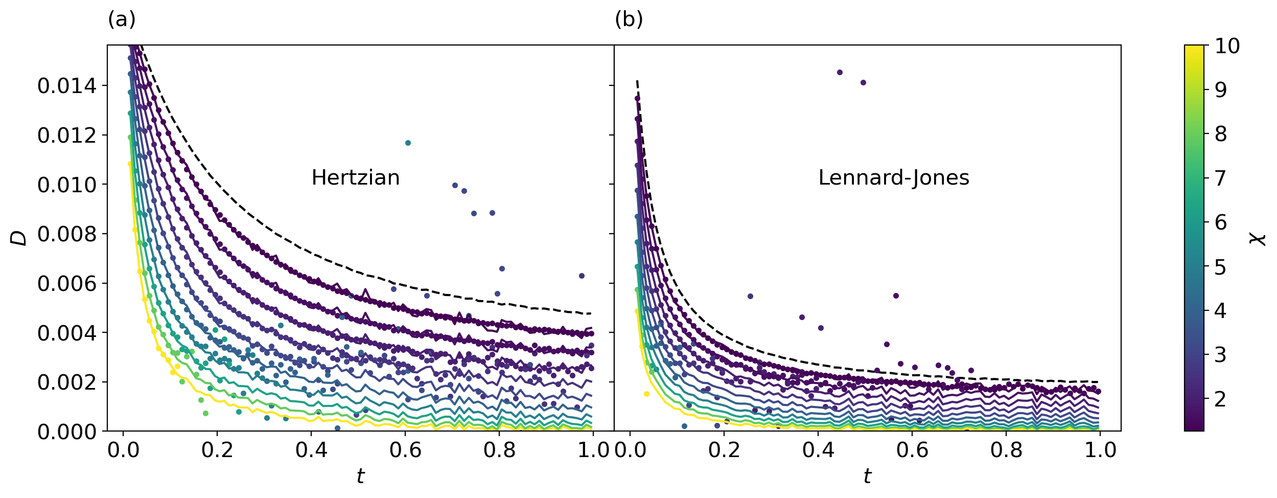
Refer to caption
Figure 10: Instantaneous diffusion coefficient calculated for both the Hertzian (a) and Lennard-Jones (b) models, at kBT=101subscript𝑘𝐵𝑇superscript101k_{B}T=10^{-1}. Prediction points are plotted as dots, and validation as solid lines. Y-scales in both plots are shared. The predictions appear to breakdown at a fixed diffusion rate of about D0.003similar-to𝐷0.003D\sim 0.003 that is independent of the potential employed.

Lastly, we examine how these behaviors change through lowering ϵ~~italic-ϵ\tilde{\epsilon} and kBTsubscript𝑘𝐵𝑇k_{B}T simultaneously by an order of magnitude. By reducing the temperature of the system to kBT=102subscript𝑘𝐵𝑇superscript102k_{B}T=10^{-2}, we observe improved accuracy in our results given the same length of time in our simulations at kBT=101subscript𝑘𝐵𝑇superscript101k_{B}T=10^{-1}. In Figure 11(a,b), our predictions track almost perfectly at all observed χ𝜒\chi for both the Hertzian and Lennard-Jones models. Though this is mostly unsurprising, as we expect this equal reduction in the temperature and energy scale to yield a similar effective temperature of simulations and push our observations out farther in time. In Figure 11(c,d), we find that the threshold D𝐷D in which we observed the breakdown in our predictions is further reduced by an order of magnitude, matching well with our reduction in temperature. This is a curious result, as it seems that this method of modeling possesses an inherent limitation on the slow dynamical processes we can resolve that is dependent on our choices of temperature and realizations employed.
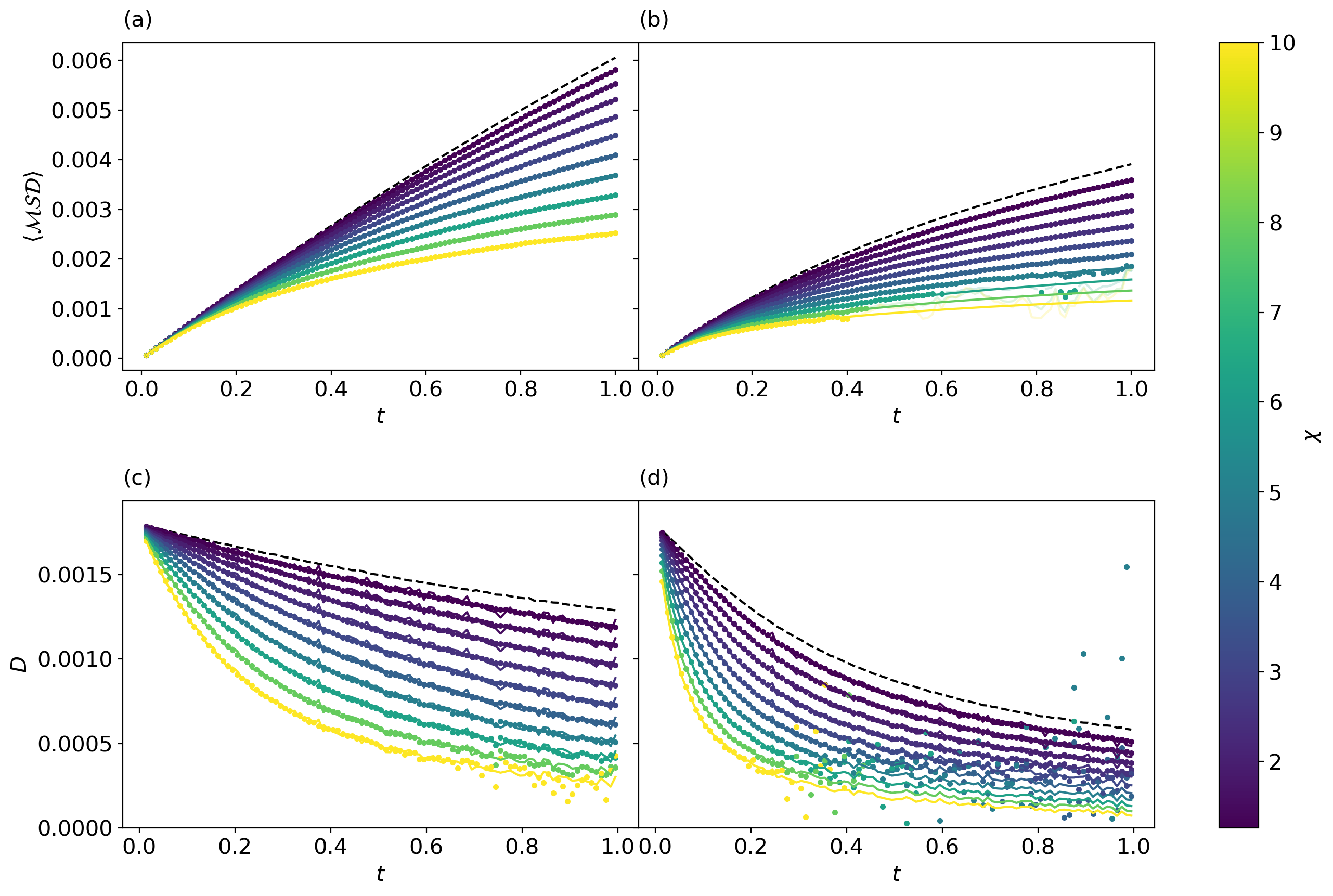
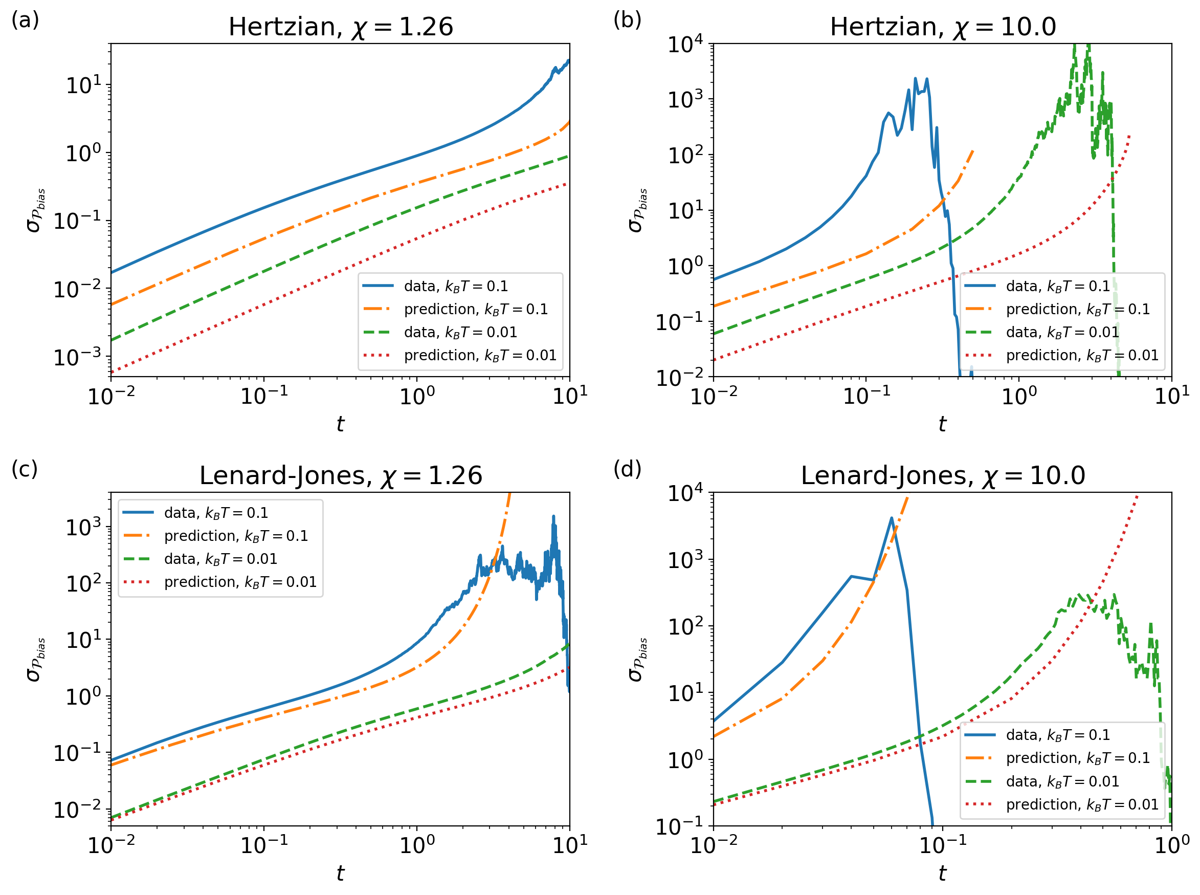
Refer to caption
Figure 11: 𝒮𝒟𝒮𝒟\mathcal{MSD} for the Hertzian (a) and Lennard-Jones (b) models, at kBT=102subscript𝑘𝐵𝑇superscript102k_{B}T=10^{-2}. Corresponding instantaneous diffusion coefficient in the Hertzian (c) and Lennard-Jones (d) models. Y-scales in both sets of plots are shared. In all cases, prediction points are plotted as dots, and validation as solid lines.
Refer to caption
Figure 12: Validation of the uncertainty estimates for the Hertzian potential with (a) χ=1.26𝜒1.26\chi=1.26, (b) χ=10𝜒10\chi=10, and for the Lennard-Jones potential with (c) χ=1.26𝜒1.26\chi=1.26, (d) χ=10𝜒10\chi=10. The time discretization for these estimates is set as nT=100subscript𝑛𝑇100n_{T}=100 and the reference trajectory is chosen as the initial configuration.

5.3 Uncertainty quantification

In the following, we compare the UQ estimates for the standard deviation of 𝒫biassubscript𝒫𝑏𝑖𝑎𝑠\mathcal{P}_{bias} with the data, for the two extreme biases considered, i.e., χ=1.26𝜒1.26\chi=1.26 and χ=10.0𝜒10.0\chi=10.0, of the Hertzian and the Lennard-Jones systems. These are shown in Figure 12 for both temperatures studied, i.e., kBT=0.1subscript𝑘𝐵𝑇0.1k_{B}T=0.1 and kBT=0.01subscript𝑘𝐵𝑇0.01k_{B}T=0.01. Here, we use nT=100subscript𝑛𝑇100n_{T}=100 for the time discretization and choose the initial (equilibrium) configuration as the reference trajectory. We recall that such estimates were built upon a quadratic approximation of the bias potential, while the biases for the systems considered are themselves Hertzian and Lennard-Jones. These potentials deviate from simple quadratic forms, particularly the Hertzian, which does not have a unique minimum but rather an extended zero plateau beyond a certain threshold. Moreover, the phenomenon here studied is that of diffusion, whereby particle trajectories will visit all parts of the potential, as opposed to be constrained to the neighborhood of a given position. Yet, despite all these rather unfavorable circumstances, the UQ estimates provide remarkably good predictions of the Lennard-Jones system, and mostly results within the same order of magnitude for the Hertzian system. To be more specific, we provide in Table 1 below the ratio between the data and the predictions for σ𝒫biassubscript𝜎subscript𝒫𝑏𝑖𝑎𝑠\sigma_{\mathcal{P}_{bias}} at two significant times of the predictions for all cases shown in Figure 12. These times are chosen to be the lowest time depicted (t=102𝑡superscript102t=10^{-2}) and the time prior to the plateau and subsequent decay of the standard deviation of 𝒫biassubscript𝒫𝑏𝑖𝑎𝑠\mathcal{P}_{bias} observed in the data (this time is case dependent, and hence specified in the table). This behavior is a strong signature of the reduced number of relevant trajectories participating in the ensemble averages, which in turn implies that the estimate of σ𝒫biassubscript𝜎subscript𝒫𝑏𝑖𝑎𝑠\sigma_{\mathcal{P}_{bias}} obtained from the data ceases to be accurate. Comparisons between the data and the predictions beyond this point are therefore not meaningful.

σ𝒫bias(data)/σ𝒫bias(predictions)subscript𝜎subscript𝒫𝑏𝑖𝑎𝑠datasubscript𝜎subscript𝒫𝑏𝑖𝑎𝑠predictions\sigma_{\mathcal{P}_{bias}}(\text{data})/\sigma_{\mathcal{P}_{bias}}(\text{predictions})
χ=1.26𝜒1.26\chi=1.26 χ=10.0𝜒10.0\chi=10.0
low time large time low time large time
Lennard-Jones kBT=0.01subscript𝑘𝐵𝑇0.01k_{B}T=0.01 1.10 (t=0.01𝑡0.01t=0.01) 2.60 (t=10𝑡10t=10) 1.12 (t=𝑡absentt=0.01) 2.84 (t=0.3𝑡0.3t=0.3)
kBT=0.1subscript𝑘𝐵𝑇0.1k_{B}T=0.1 1.34 (t=0.01𝑡0.01t=0.01) 2.69 (t=1𝑡1t=1) 1.70 (t=0.01𝑡0.01t=0.01) 5.29 (t=0.03𝑡0.03t=0.03)
Hertzian kBT=0.01subscript𝑘𝐵𝑇0.01k_{B}T=0.01 2.97 (t=0.01𝑡0.01t=0.01) 2.52 (t=10𝑡10t=10) 2.96 (t=0.01𝑡0.01t=0.01) 23.5 (t=1𝑡1t=1)
kBT=0.1subscript𝑘𝐵𝑇0.1k_{B}T=0.1 2.95 (t=0.01𝑡0.01t=0.01) 8.10 (t=10𝑡10t=10) 3.02 (t=0.01𝑡0.01t=0.01) 25.2 (t=0.1𝑡0.1t=0.1)
Table 1: Ratio of the standard deviation of 𝒫biassubscript𝒫𝑏𝑖𝑎𝑠\mathcal{P}_{bias} between the data and UQ prediction for the Lenard-Jones and Hertzian potentials.

Finally, we make some remarks regarding the computation of the UQ estimates. These calculations were found to be extremely fast and only requiring about a minute for each case in Matlab on a laptop. This is for the time discretization used, nT=100subscript𝑛𝑇100n_{T}=100, which was sufficient to guarantee convergence in all cases, and for similar-to\sim100 time points. Yet, it is important to remark that, as the difference between the target and simulated potentials increases, or as time increases, the spectrum of the eigenvalues of matrix 𝐀sqsubscript𝐀𝑠𝑞\mathbf{A}_{sq} become increasingly large, which can lead to a poorly conditioned matrix and associated numerical issues. Indeed, a direct evaluation of Eq. (25) using Matlab, will not produce results after a given time, as could be implied from Figure 12. Although these numerical issues could be potentially resolved by recourse to more sophisticated strategies, these were not pursued here, as the time range of the predictions already surpassed the point of failure of the path reweighting strategy.

6 Conclusions

In this paper, we provide a statistical mechanics approach with quantified uncertainty to extrapolate material behavior to distinct loading conditions or material systems. The approach is based on the reweighting of the probability density for trajectories, building up on the ideas of [1], and enables the calculation of ensemble averages of arbitrary observables of system/process S𝑆S from simulations (or, potentially, experimental data) of system/process S~~𝑆\tilde{S}. The formalism is a priori exact and possess many attractive features, such as acceleration of the dynamics under a suitable choice of bias potential, enabling trivial time parallelization, or the full exploration of a family of potentials at virtually zero added computational cost. Yet, it suffers from sampling issues as the “distance” between the predicted and simulated system increase, which become more apparent for large times or large particulate systems. In other words, for a fixed number of realizations of system S~~𝑆\tilde{S}, the uncertainty in the predictions for S𝑆S become increasingly large with the bias potential for a fixed time, or with time, for a fixed bias potential. Remarkably though, the uncertainty of such predictions can be estimated a priori without requiring any simulations of S𝑆S. Specifically, analytical formulas for estimating the uncertainty were here derived based on a quadratic approximation of the bias potential (difference between the potential of systems S~~𝑆\tilde{S} and S𝑆S). These estimates proved to be remarkably accurate for systems with a strong quadratic bias (and markedly more accurate than classical formulas for the propagation of uncertainty), and deliver estimates for the errors within the good order of magnitude for realistic potentials.

The above path reweighting strategy and uncertainty quantification estimates have been applied to two illustrative examples. The first example is a one-dimensional mass-spring chain, often used as prototype for polymer chains or biological macromolecules. This simple example is used to showcase the versatility of the approach, both, in the type of observables that can be predicted (microscopic or macroscopic, and instantaneous or path dependent), and the types of inference that can be made from one system to another (e.g., from one potential to another, from equilibrium to non-equilibrium, or the extreme case of predicting the non-equilibrium behavior of an interacting particle system from independent Brownian particles). The second example, is a two-dimensional glass-former system with Hertzian or Lennard-Jones potential, where the emergence of particle caging is predicted from the liquid phase as the strength of the potential is increased. These two rather distinct examples (one elastic and the other diffusive) illustrate the possibility of extrapolating under far-from-equilibrium conditions with a high degree of accuracy for small systems and short times.

7 Acknowledgements

The authors gratefully acknowledge support from ACS, USA PRF 61793-ND10 Grant (S. H.) and from NSF CAREER Award, CMMI-2047506 (C. R). S. F. acknowledges support from the UK EPSRC, grant no. EP/R005974/1, and helpful discussions with Profs. T. Ala-Nissilä and A. Archer. I. G. and P. E. A. acknowledge support from NSF DMR (Penn MRSEC) 1720530.

Appendix A Path integral representation of Langevin dynamics

We here consider the main equation discussed in the narrative, mainly,

ηx˙=Vx+σξ˙,𝜂˙𝑥𝑉𝑥𝜎˙𝜉\eta\dot{x}=-\frac{\partial V}{\partial x}+\sqrt{\sigma}\,\dot{\xi}, (37)

where, for convenience, we restrict ourselves to the one dimensional case, and denote σ=2kBTη𝜎2subscript𝑘𝐵𝑇𝜂\sigma=2k_{B}T\eta. This stochastic differential equation has additive noise, i.e., σ𝜎\sigma is independent of x𝑥x, and hence, its Itô and Stratonovich interpretation coincide.

In this appendix we derive the path integral representation of Eq. (37) [42, 3], following both the Itô and Stratonovich interpretation, and demonstrate their equivalence.

Beginning with the Itô interpretation, we discretize Eq. (37) with a constant time step ΔtΔ𝑡\Delta t, according to the Euler-Maruyama scheme

η(xn+1xn)=V(xn)Δt+σ(ξn+1ξn),𝜂superscript𝑥𝑛1superscript𝑥𝑛superscript𝑉superscript𝑥𝑛Δ𝑡𝜎superscript𝜉𝑛1superscript𝜉𝑛\eta(x^{n+1}-x^{n})=-V^{\prime}(x^{n})\Delta t+\sqrt{\sigma}(\xi^{n+1}-\xi^{n}), (38)

where the superscript n+1𝑛1n+1 is associated to time step tn+1=tn+Δtsuperscript𝑡𝑛1superscript𝑡𝑛Δ𝑡t^{n+1}=t^{n}+\Delta t and V=V/xsuperscript𝑉𝑉𝑥V^{\prime}=\partial V/\partial x. Then, the probability of seeing a trajectory {x}0nT{x0,x1,.,xnT}\{x\}_{0}^{n_{T}}\coloneqq\{x^{0},x^{1},....,x^{n_{T}}\} given the initial conditions, is given by the product of the transition probabilities

𝒫({x}0nT|x0)=n=0nT1Qn(n+1,n)Qn(n+1,n)=1Znexp[12σ(ηxn+1xnΔt+V(xn))2Δt],𝒫conditionalsuperscriptsubscript𝑥0subscript𝑛𝑇superscript𝑥0superscriptsubscriptproduct𝑛0subscript𝑛𝑇1subscript𝑄𝑛𝑛1𝑛subscript𝑄𝑛𝑛1𝑛1superscript𝑍𝑛12𝜎superscript𝜂superscript𝑥𝑛1superscript𝑥𝑛Δ𝑡superscript𝑉superscript𝑥𝑛2Δ𝑡\begin{split}&\mathcal{P}\left(\{x\}_{0}^{n_{T}}|x^{0}\right)=\prod_{n=0}^{n_{T}-1}Q_{n}(n+1,n)\\ &Q_{n}(n+1,n)=\frac{1}{Z^{n}}\exp\left[-\frac{1}{2\sigma}\left(\eta\frac{x^{n+1}-x^{n}}{\Delta t}+V^{\prime}(x^{n})\right)^{2}\Delta t\right],\end{split} (39)

where the factors Znsuperscript𝑍𝑛Z^{n} must ensure that the probability distribution is normalized to 1, i.e.,

Zn=exp[12σ(ηxn+1xnΔt+V(xn))2Δt]𝑑xn+1.superscript𝑍𝑛superscriptsubscript12𝜎superscript𝜂superscript𝑥𝑛1superscript𝑥𝑛Δ𝑡superscript𝑉superscript𝑥𝑛2Δ𝑡differential-dsuperscript𝑥𝑛1Z^{n}=\int_{-\infty}^{\infty}\exp\left[-\frac{1}{2\sigma}\left(\eta\frac{x^{n+1}-x^{n}}{\Delta t}+V^{\prime}(x^{n})\right)^{2}\Delta t\right]\,dx^{n+1}. (40)

These are simple Gaussian integrals, which can be readily computed as

Zn=2πσΔtη.superscript𝑍𝑛2𝜋𝜎Δ𝑡𝜂Z^{n}=\frac{\sqrt{2\pi\sigma\Delta t}}{\eta}. (41)

Hence, the path probability distribution reads

𝒫({x}0nT|x0)=(n=0nT1η2πσΔt)exp[12σn=0nT1(ηxn+1xnΔt+V(xn))2Δt],𝒫conditionalsuperscriptsubscript𝑥0subscript𝑛𝑇superscript𝑥0superscriptsubscriptproduct𝑛0subscript𝑛𝑇1𝜂2𝜋𝜎Δ𝑡12𝜎superscriptsubscript𝑛0subscript𝑛𝑇1superscript𝜂superscript𝑥𝑛1superscript𝑥𝑛Δ𝑡superscript𝑉superscript𝑥𝑛2Δ𝑡\mathcal{P}\left(\{x\}_{0}^{n_{T}}|x^{0}\right)=\left(\prod_{n=0}^{n_{T}-1}\frac{\eta}{\sqrt{2\pi\sigma\Delta t}}\right)\exp\left[-\frac{1}{2\sigma}\sum_{n=0}^{n_{T}-1}\left(\eta\frac{x^{n+1}-x^{n}}{\Delta t}+V^{\prime}(x^{n})\right)^{2}\Delta t\right], (42)

or equivalently,

𝒫({x}0nT|x0)=(n=0nT1η2πσΔt)eβ,with=14ηn=0nT1(ηxn+1xnΔt+V(xn))2Δt.formulae-sequence𝒫conditionalsuperscriptsubscript𝑥0subscript𝑛𝑇superscript𝑥0superscriptsubscriptproduct𝑛0subscript𝑛𝑇1𝜂2𝜋𝜎Δ𝑡superscript𝑒𝛽with14𝜂superscriptsubscript𝑛0subscript𝑛𝑇1superscript𝜂superscript𝑥𝑛1superscript𝑥𝑛Δ𝑡superscript𝑉superscript𝑥𝑛2Δ𝑡\mathcal{P}\left(\{x\}_{0}^{n_{T}}|x^{0}\right)=\left(\prod_{n=0}^{n_{T}-1}\frac{\eta}{\sqrt{2\pi\sigma\Delta t}}\right)e^{-\beta\mathcal{I}},\quad\text{with}\quad\mathcal{I}=\frac{1}{4\eta}\sum_{n=0}^{n_{T}-1}\left(\eta\frac{x^{n+1}-x^{n}}{\Delta t}+V^{\prime}(x^{n})\right)^{2}\Delta t. (43)

If, in contrast, we had started with a Stratonovich interpretation of Eq. (37), then, its discretized version would read

η(xn+1xn)=V(xn+1/2)Δt+σ(ξn+1ξn),𝜂superscript𝑥𝑛1superscript𝑥𝑛superscript𝑉superscript𝑥𝑛12Δ𝑡𝜎superscript𝜉𝑛1superscript𝜉𝑛\eta(x^{n+1}-x^{n})=-V^{\prime}(x^{n+1/2})\Delta t+\sqrt{\sigma}(\xi^{n+1}-\xi^{n}), (44)

where xn+1/2superscript𝑥𝑛12x^{n+1/2} is defined as xn+1+xn2superscript𝑥𝑛1superscript𝑥𝑛2\frac{x^{n+1}+x^{n}}{2}. The probability of observing a trajectory would then be expressed as

𝒫({x}0nT|x0)=n=0nT1Qn(n+1,n),withQn(n+1,n)=1Znexp[12σ(ηxn+1xnΔt+V(xn+1/2))2Δt].formulae-sequence𝒫conditionalsuperscriptsubscript𝑥0subscript𝑛𝑇superscript𝑥0superscriptsubscriptproduct𝑛0subscript𝑛𝑇1subscript𝑄𝑛𝑛1𝑛withsubscript𝑄𝑛𝑛1𝑛1superscript𝑍𝑛12𝜎superscript𝜂superscript𝑥𝑛1superscript𝑥𝑛Δ𝑡superscript𝑉superscript𝑥𝑛122Δ𝑡\begin{split}&\mathcal{P}\left(\{x\}_{0}^{n_{T}}|x^{0}\right)=\prod_{n=0}^{n_{T}-1}Q_{n}(n+1,n),\quad\text{with}\\ &Q_{n}(n+1,n)=\frac{1}{Z^{n}}\exp\left[-\frac{1}{2\sigma}\left(\eta\frac{x^{n+1}-x^{n}}{\Delta t}+V^{\prime}(x^{n+1/2})\right)^{2}\Delta t\right].\end{split} (45)

Similarly, the normalization factors Znsuperscript𝑍𝑛Z^{n} must satisfy

Zn=exp[12σ(ηxn+1xnΔt+V(xn+1/2))2Δt]𝑑xn+1.superscript𝑍𝑛superscriptsubscript12𝜎superscript𝜂superscript𝑥𝑛1superscript𝑥𝑛Δ𝑡superscript𝑉superscript𝑥𝑛122Δ𝑡differential-dsuperscript𝑥𝑛1Z^{n}=\int_{-\infty}^{\infty}\exp\left[-\frac{1}{2\sigma}\left(\eta\frac{x^{n+1}-x^{n}}{\Delta t}+V^{\prime}(x^{n+1/2})\right)^{2}\Delta t\right]\,dx^{n+1}. (46)

We approximate this integral by doing a Taylor expansion of V(xn+1/2)superscript𝑉superscript𝑥𝑛12V^{\prime}(x^{n+1/2}) around xnsuperscript𝑥𝑛x^{n}, as

V(xn+1/2)V(xn)+V′′(xn)(xn+1/2xn)V(xn)+V′′(xn)xn+1xn2.similar-to-or-equalssuperscript𝑉superscript𝑥𝑛12superscript𝑉superscript𝑥𝑛superscript𝑉′′superscript𝑥𝑛superscript𝑥𝑛12superscript𝑥𝑛similar-to-or-equalssuperscript𝑉superscript𝑥𝑛superscript𝑉′′superscript𝑥𝑛superscript𝑥𝑛1superscript𝑥𝑛2V^{\prime}(x^{n+1/2})\simeq V^{\prime}(x^{n})+V^{\prime\prime}(x^{n})\left(x^{n+1/2}-x^{n}\right)\simeq V^{\prime}(x^{n})+V^{\prime\prime}(x^{n})\frac{x^{n+1}-x^{n}}{2}. (47)

Then, a simple Gaussian integration delivers

Zn2πσΔtη(1+V′′(xn)Δt2η).similar-to-or-equalssuperscript𝑍𝑛2𝜋𝜎Δ𝑡𝜂1superscript𝑉′′superscript𝑥𝑛Δ𝑡2𝜂Z^{n}\simeq\frac{\sqrt{2\pi\sigma\Delta t}}{\eta\left(1+V^{\prime\prime}(x^{n})\frac{\Delta t}{2\eta}\right)}. (48)

The term in parenthesis may be further approximated by an exponential, and similarly, V′′superscript𝑉′′V^{\prime\prime} may be evaluated at xn+1/2superscript𝑥𝑛12x^{n+1/2} to first order, i.e.

Zn2πσΔtηexp[12ηV′′(xn+1/2)Δt].similar-to-or-equalssuperscript𝑍𝑛2𝜋𝜎Δ𝑡𝜂12𝜂superscript𝑉′′superscript𝑥𝑛12Δ𝑡Z^{n}\simeq\frac{\sqrt{2\pi\sigma\Delta t}}{\eta}\exp\left[-\frac{1}{2\eta}V^{\prime\prime}(x^{n+1/2})\Delta t\right]. (49)

The path probability distribution (to first order in ΔtΔ𝑡\Delta t in the exponential) may then be expressed as

𝒫({x}0nT|x0)=(n=0nT1η2πσΔt)exp[12σn=0nT1(ηxn+1xnΔt+V(xn+1/2))2Δt+12ηV′′(xn+1/2)Δt].𝒫conditionalsuperscriptsubscript𝑥0subscript𝑛𝑇superscript𝑥0superscriptsubscriptproduct𝑛0subscript𝑛𝑇1𝜂2𝜋𝜎Δ𝑡12𝜎superscriptsubscript𝑛0subscript𝑛𝑇1superscript𝜂superscript𝑥𝑛1superscript𝑥𝑛Δ𝑡superscript𝑉superscript𝑥𝑛122Δ𝑡12𝜂superscript𝑉′′superscript𝑥𝑛12Δ𝑡\mathcal{P}\left(\{x\}_{0}^{n_{T}}|x^{0}\right)=\left(\prod_{n=0}^{n_{T}-1}\frac{\eta}{\sqrt{2\pi\sigma\Delta t}}\right)\exp\left[-\frac{1}{2\sigma}\sum_{n=0}^{n_{T}-1}\left(\eta\frac{x^{n+1}-x^{n}}{\Delta t}+V^{\prime}(x^{n+1/2})\right)^{2}\Delta t+\frac{1}{2\eta}V^{\prime\prime}(x^{n+1/2})\Delta t\right]. (50)

Although this expression is, in appearance, distinct to Eq. (42), their exponents are actually identical to first order in ΔtΔ𝑡\Delta t. Indeed, after expanding the squares in (50), the cross term is the only one that requires special consideration. In particular, from Itô’s formula, it follows that

2ηxn+1xnΔtV(xn+1/2)2ηxn+1xnΔtV(xn)+2ηxn+1xnΔtV′′(xn)xn+1xn2+𝒪(Δt)2ηxn+1xnΔtV(xn)+σηV′′(xn)+𝒪(Δt).similar-to-or-equals2𝜂superscript𝑥𝑛1superscript𝑥𝑛Δ𝑡superscript𝑉superscript𝑥𝑛122𝜂superscript𝑥𝑛1superscript𝑥𝑛Δ𝑡superscript𝑉superscript𝑥𝑛2𝜂superscript𝑥𝑛1superscript𝑥𝑛Δ𝑡superscript𝑉′′superscript𝑥𝑛superscript𝑥𝑛1superscript𝑥𝑛2𝒪Δ𝑡similar-to-or-equals2𝜂superscript𝑥𝑛1superscript𝑥𝑛Δ𝑡superscript𝑉superscript𝑥𝑛𝜎𝜂superscript𝑉′′superscript𝑥𝑛𝒪Δ𝑡\begin{split}2\eta\frac{x^{n+1}-x^{n}}{\Delta t}V^{\prime}(x^{n+1/2})&\simeq 2\eta\frac{x^{n+1}-x^{n}}{\Delta t}V^{\prime}(x^{n})+2\eta\frac{x^{n+1}-x^{n}}{\Delta t}V^{\prime\prime}(x^{n})\frac{x^{n+1}-x^{n}}{2}+\mathcal{O}(\sqrt{\Delta t})\\ &\simeq 2\eta\frac{x^{n+1}-x^{n}}{\Delta t}V^{\prime}(x^{n})+\frac{\sigma}{\eta}V^{\prime\prime}(x^{n})+\mathcal{O}(\sqrt{\Delta t}).\end{split} (51)

The second term involving V′′(xn)superscript𝑉′′superscript𝑥𝑛V^{\prime\prime}(x^{n}) then cancels with the last term in the exponent of Eq. (50), recovering Eq. (42). In views of its simplicity, Eq. (42) is chosen for implementation purposes, as well as in the derivations in the following appendices.

Appendix B Path integral transformation under change of potential

Following the discrete representation of the path integrals in Itô form used in A, we here prove Eq. (4), for N=1𝑁1N=1 in one dimension, without lost of generality. Towards that goal, we define Vbias=V~Vsubscript𝑉𝑏𝑖𝑎𝑠~𝑉𝑉V_{bias}=\tilde{V}-V and replace V𝑉V by V~Vbias~𝑉subscript𝑉𝑏𝑖𝑎𝑠\tilde{V}-V_{bias} in the rate functional biassubscript𝑏𝑖𝑎𝑠\mathcal{I}_{bias} of Eq. (43), and expand the squares as

=14ηn=0nT1(ηxn+1xnΔt+V~(xn)Vbias(xn))2Δt=14ηn=0nT1[(ηxn+1xnΔt+V~(xn))2+(Vbias(xn))22Vbias(xn)(ηxn+1xnΔt+V~(xn))]Δt.14𝜂superscriptsubscript𝑛0subscript𝑛𝑇1superscript𝜂superscript𝑥𝑛1superscript𝑥𝑛Δ𝑡superscript~𝑉superscript𝑥𝑛subscriptsuperscript𝑉𝑏𝑖𝑎𝑠superscript𝑥𝑛2Δ𝑡14𝜂superscriptsubscript𝑛0subscript𝑛𝑇1delimited-[]superscript𝜂superscript𝑥𝑛1superscript𝑥𝑛Δ𝑡superscript~𝑉superscript𝑥𝑛2superscriptsubscriptsuperscript𝑉𝑏𝑖𝑎𝑠superscript𝑥𝑛22subscriptsuperscript𝑉𝑏𝑖𝑎𝑠superscript𝑥𝑛𝜂superscript𝑥𝑛1superscript𝑥𝑛Δ𝑡superscript~𝑉superscript𝑥𝑛Δ𝑡\begin{split}\mathcal{I}&=\frac{1}{4\eta}\sum_{n=0}^{n_{T}-1}\left(\eta\frac{x^{n+1}-x^{n}}{\Delta t}+\tilde{V}^{\prime}(x^{n})-V^{\prime}_{bias}(x^{n})\right)^{2}\Delta t\\ &=\frac{1}{4\eta}\sum_{n=0}^{n_{T}-1}\left[\left(\eta\frac{x^{n+1}-x^{n}}{\Delta t}+\tilde{V}^{\prime}(x^{n})\right)^{2}+\left(V^{\prime}_{bias}(x^{n})\right)^{2}-2V^{\prime}_{bias}(x^{n})\left(\eta\frac{x^{n+1}-x^{n}}{\Delta t}+\tilde{V}^{\prime}(x^{n})\right)\right]\Delta t.\end{split} (52)

Here, ~~\tilde{\mathcal{I}} may be readily identified in the first term, and hence

bias=~=14ηn=0nT1Vbias(xn)[Vbias(xn)Δt22kBTη(ξn+1ξn)],subscript𝑏𝑖𝑎𝑠~14𝜂superscriptsubscript𝑛0subscript𝑛𝑇1subscriptsuperscript𝑉𝑏𝑖𝑎𝑠superscript𝑥𝑛delimited-[]subscriptsuperscript𝑉𝑏𝑖𝑎𝑠superscript𝑥𝑛Δ𝑡22subscript𝑘𝐵𝑇𝜂superscript𝜉𝑛1superscript𝜉𝑛\mathcal{I}_{bias}=\mathcal{I}-\mathcal{\tilde{I}}=\frac{1}{4\eta}\sum_{n=0}^{n_{T}-1}V^{\prime}_{bias}(x^{n})\left[V^{\prime}_{bias}(x^{n})\Delta t-2\sqrt{2k_{B}T\eta}\left(\xi^{n+1}-\xi^{n}\right)\right], (53)

where we have used the Langevin equation associated to V~~𝑉\tilde{V}.

Appendix C Nonlinear uncertainty quantification estimate

In this appendix we provide the detailed calculations that lead to the variance estimate for 𝒫biassubscript𝒫𝑏𝑖𝑎𝑠\mathcal{P}_{bias}, given by Eq. (25) in the narrative.

We begin by deriving an approximation for 𝒫biassubscript𝒫𝑏𝑖𝑎𝑠\mathcal{P}_{bias} resulting from the expansions given in Eqs. (12) and (13). Directly inserting such expansions into the integrand of biassubscript𝑏𝑖𝑎𝑠\mathcal{I}_{bias}, this may be approximated as

Vbias(𝐱n,tn)(Vbias(𝐱n,tn)Δt2σΔ𝝃n)Vbias|𝐱rn(t)+Vbias|𝐱rn(t)δ𝐱n2Δt2(Vbias|𝐱rn(t)+Vbias|𝐱rn(t)δ𝐱n)[η(Δ𝐱rn+δ𝐱n+1δ𝐱n)+V~|𝐱rnΔt+V~|𝐱rnδ𝐱nΔt]\begin{split}&\nabla V_{bias}(\mathbf{x}^{n},t^{n})\cdot\left(\nabla V_{bias}(\mathbf{x}^{n},t^{n})\Delta t-2\sqrt{\sigma}\Delta\bm{\xi}^{n}\right)\\ &\simeq\left\|\left.\nabla V_{bias}\right|_{\mathbf{x}_{r}^{n}(t)}+\left.\nabla\nabla V_{bias}\right|_{\mathbf{x}_{r}^{n}(t)}\delta\mathbf{x}^{n}\right\|^{2}\Delta t\\ &\quad-2\left(\left.\nabla V_{bias}\right|_{\mathbf{x}_{r}^{n}(t)}+\left.\nabla\nabla V_{bias}\right|_{\mathbf{x}_{r}^{n}(t)}\delta\mathbf{x}^{n}\right)\cdot\left[\eta\left(\Delta\mathbf{x}^{n}_{r}+\delta\mathbf{x}^{n+1}-\delta\mathbf{x}^{n}\right)+\left.\nabla\tilde{V}\right|_{\mathbf{x}_{r}^{n}}\Delta t+\left.\nabla\nabla\tilde{V}\right|_{\mathbf{x}_{r}^{n}}\delta\mathbf{x}^{n}\Delta t\right]\end{split} (54)

Expanding the products, and noting that VbiasV~=Vsubscript𝑉𝑏𝑖𝑎𝑠~𝑉𝑉V_{bias}-\tilde{V}=-V,

Vbias(𝐱n,tn)(Vbias(𝐱n,tn)Δt2σΔ𝝃n)Vbias|𝐱rn(t)2Δt2Vbias|𝐱rn(t)[ηΔ𝐱rn+V~|𝐱rnΔt]+2Vbias|𝐱rn(t)(Vbias|𝐱rn(t)δ𝐱nΔt)2Vbias|𝐱rn(t)[η(δ𝐱n+1δ𝐱n)+V~|𝐱rnδ𝐱nΔt]2(Vbias|𝐱rn(t)δ𝐱n)[ηΔ𝐱rn+V~|𝐱rnΔt]2(Vbias|𝐱rn(t)δ𝐱n)[η(δ𝐱n+1δ𝐱n)+V~|𝐱rnδ𝐱nΔt]+Vbias|𝐱rn(t)δ𝐱n2Δt=Vbias|𝐱rn(t)2Δt2Vbias|𝐱rn(t)[ηΔ𝐱rn+V~|𝐱rnΔt]2Vbias|𝐱rn(t)[η(δ𝐱n+1δ𝐱n)+V|𝐱rnδ𝐱nΔt]2(Vbias|𝐱rn(t)δ𝐱n)[ηΔ𝐱rn+V~|𝐱rnΔt]2(Vbias|𝐱rn(t)δ𝐱n)[η(δ𝐱n+1δ𝐱n)+V~|𝐱rnδ𝐱nΔt]+Vbias|𝐱rn(t)δ𝐱n2Δt\begin{split}&\nabla V_{bias}(\mathbf{x}^{n},t^{n})\cdot\left(\nabla V_{bias}(\mathbf{x}^{n},t^{n})\Delta t-2\sqrt{\sigma}\Delta\bm{\xi}^{n}\right)\\ &\simeq\left\|\left.\nabla V_{bias}\right|_{\mathbf{x}_{r}^{n}(t)}\right\|^{2}\Delta t-2\left.\nabla V_{bias}\right|_{\mathbf{x}_{r}^{n}(t)}\cdot\left[\eta\Delta\mathbf{x}^{n}_{r}+\left.\nabla\tilde{V}\right|_{\mathbf{x}_{r}^{n}}\Delta t\right]\\ &\quad+2\left.\nabla V_{bias}\right|_{\mathbf{x}_{r}^{n}(t)}\cdot\left(\left.\nabla\nabla V_{bias}\right|_{\mathbf{x}_{r}^{n}(t)}\delta\mathbf{x}^{n}\Delta t\right)\\ &\quad-2\left.\nabla V_{bias}\right|_{\mathbf{x}_{r}^{n}(t)}\cdot\left[\eta\left(\delta\mathbf{x}^{n+1}-\delta\mathbf{x}^{n}\right)+\left.\nabla\nabla\tilde{V}\right|_{\mathbf{x}_{r}^{n}}\delta\mathbf{x}^{n}\Delta t\right]-2\left(\left.\nabla\nabla V_{bias}\right|_{\mathbf{x}_{r}^{n}(t)}\delta\mathbf{x}^{n}\right)\cdot\left[\eta\Delta\mathbf{x}^{n}_{r}+\left.\nabla\tilde{V}\right|_{\mathbf{x}_{r}^{n}}\Delta t\right]\\ &\quad-2\left(\left.\nabla\nabla V_{bias}\right|_{\mathbf{x}_{r}^{n}(t)}\delta\mathbf{x}^{n}\right)\cdot\left[\eta\left(\delta\mathbf{x}^{n+1}-\delta\mathbf{x}^{n}\right)+\left.\nabla\nabla\tilde{V}\right|_{\mathbf{x}_{r}^{n}}\delta\mathbf{x}^{n}\Delta t\right]\\ &\quad+\left\|\left.\nabla\nabla V_{bias}\right|_{\mathbf{x}_{r}^{n}(t)}\delta\mathbf{x}^{n}\right\|^{2}\Delta t\\ &=\left\|\left.\nabla V_{bias}\right|_{\mathbf{x}_{r}^{n}(t)}\right\|^{2}\Delta t-2\left.\nabla V_{bias}\right|_{\mathbf{x}_{r}^{n}(t)}\cdot\left[\eta\Delta\mathbf{x}^{n}_{r}+\left.\nabla\tilde{V}\right|_{\mathbf{x}_{r}^{n}}\Delta t\right]\\ &\quad-2\left.\nabla V_{bias}\right|_{\mathbf{x}_{r}^{n}(t)}\cdot\left[\eta\left(\delta\mathbf{x}^{n+1}-\delta\mathbf{x}^{n}\right)+\left.\nabla\nabla V\right|_{\mathbf{x}_{r}^{n}}\delta\mathbf{x}^{n}\Delta t\right]-2\left(\left.\nabla\nabla V_{bias}\right|_{\mathbf{x}_{r}^{n}(t)}\delta\mathbf{x}^{n}\right)\cdot\left[\eta\Delta\mathbf{x}^{n}_{r}+\left.\nabla\tilde{V}\right|_{\mathbf{x}_{r}^{n}}\Delta t\right]\\ &\quad-2\left(\left.\nabla\nabla V_{bias}\right|_{\mathbf{x}_{r}^{n}(t)}\delta\mathbf{x}^{n}\right)\cdot\left[\eta\left(\delta\mathbf{x}^{n+1}-\delta\mathbf{x}^{n}\right)+\left.\nabla\nabla\tilde{V}\right|_{\mathbf{x}_{r}^{n}}\delta\mathbf{x}^{n}\Delta t\right]\\ &\quad+\left\|\left.\nabla\nabla V_{bias}\right|_{\mathbf{x}_{r}^{n}(t)}\delta\mathbf{x}^{n}\right\|^{2}\Delta t\end{split} (55)

Next, we define δ𝐲n=(η/σΔt)δ𝐱n𝛿superscript𝐲𝑛𝜂𝜎Δ𝑡𝛿superscript𝐱𝑛\delta\mathbf{y}^{n}=\left(\eta/\sqrt{\sigma\Delta t}\right)\delta\mathbf{x}^{n} and recall that form the definition of σ𝜎\sigma, β4η=12σ𝛽4𝜂12𝜎\frac{\beta}{4\eta}=\frac{1}{2\sigma}. Then, 𝒫biassubscript𝒫𝑏𝑖𝑎𝑠\mathcal{P}_{bias} may be approximately written as

𝒫bias=eβbias=exp[12σn=0nT1Vbias(𝐱n,tn)(Vbias(𝐱n,tn)Δt2σΔ𝝃n)]exp[n=0nT1{12σ[Vbias|𝐱rn22Vbias|𝐱rn(ηΔ𝐱rnΔt+V~|𝐱rn)]ΔtΔtσ[Vbias|𝐱rn(δ𝐲n+1δ𝐲n+V|𝐱rnδ𝐲nΔtη)+(Vbias|𝐱rnδ𝐲n)(Δ𝐱rn+V~|𝐱rnΔtη)]1η(Vbias|𝐱rnδ𝐲n)[δ𝐲n+1δ𝐲n+1ηV~|𝐱rnδ𝐲nΔt]Δt+12η2Vbias|𝐱rnδ𝐲n2Δt2}].\begin{split}\mathcal{P}_{bias}&=e^{-\beta\mathcal{I}_{bias}}=\exp\left[-\frac{1}{2\sigma}\sum_{n=0}^{n_{T}-1}\nabla V_{bias}(\mathbf{x}^{n},t^{n})\cdot\left(\nabla V_{bias}(\mathbf{x}^{n},t^{n})\Delta t-2\sqrt{\sigma}\Delta\bm{\xi}^{n}\right)\right]\\ &\simeq\exp\left[-\sum_{n=0}^{n_{T}-1}\left\{\frac{1}{2\sigma}\left[\left\|\left.\nabla V_{bias}\right|_{\mathbf{x}_{r}^{n}}\right\|^{2}-2\left.\nabla V_{bias}\right|_{\mathbf{x}_{r}^{n}}\cdot\left(\eta\frac{\Delta\mathbf{x}^{n}_{r}}{\Delta t}+\left.\nabla\tilde{V}\right|_{\mathbf{x}_{r}^{n}}\right)\right]\Delta t\right.\right.\\ &\quad-\sqrt{\frac{\Delta t}{\sigma}}\left[\left.\nabla V_{bias}\right|_{\mathbf{x}_{r}^{n}}\cdot\left(\delta\mathbf{y}^{n+1}-\delta\mathbf{y}^{n}+\left.\nabla\nabla V\right|_{\mathbf{x}_{r}^{n}}\delta\mathbf{y}^{n}\frac{\Delta t}{\eta}\right)+\left(\left.\nabla\nabla V_{bias}\right|_{\mathbf{x}_{r}^{n}}\delta\mathbf{y}^{n}\right)\cdot\left(\Delta\mathbf{x}^{n}_{r}+\left.\nabla\tilde{V}\right|_{\mathbf{x}_{r}^{n}}\frac{\Delta t}{\eta}\right)\right]\\ &\quad-\frac{1}{\eta}\left(\left.\nabla\nabla V_{bias}\right|_{\mathbf{x}_{r}^{n}}\delta\mathbf{y}^{n}\right)\cdot\left[\delta\mathbf{y}^{n+1}-\delta\mathbf{y}^{n}+\frac{1}{\eta}\left.\nabla\nabla\tilde{V}\right|_{\mathbf{x}_{r}^{n}}\delta\mathbf{y}^{n}\Delta t\right]\Delta t\\ &\quad\left.\left.+\frac{1}{2\eta^{2}}\left\|\left.\nabla\nabla V_{bias}\right|_{\mathbf{x}_{r}^{n}}\delta\mathbf{y}^{n}\right\|^{2}\Delta t^{2}\right\}\right].\end{split} (56)

We now assume that 𝐱r(t0)=𝟎subscript𝐱𝑟superscript𝑡00\mathbf{x}_{r}(t^{0})=\mathbf{0} such that δ𝐲0=η/(σΔt)δ𝐱0=𝟎𝛿superscript𝐲0𝜂𝜎Δ𝑡𝛿superscript𝐱00\delta\mathbf{y}^{0}=\eta/\sqrt{(\sigma\Delta t)}\delta\mathbf{x}^{0}=\mathbf{0}, and define Δ(Vbias|𝐱rn1)Vbias|𝐱rnVbias|𝐱rn1Δevaluated-atsubscript𝑉𝑏𝑖𝑎𝑠superscriptsubscript𝐱𝑟𝑛1evaluated-atsubscript𝑉𝑏𝑖𝑎𝑠superscriptsubscript𝐱𝑟𝑛evaluated-atsubscript𝑉𝑏𝑖𝑎𝑠superscriptsubscript𝐱𝑟𝑛1\Delta\left(\left.\nabla V_{bias}\right|_{\mathbf{x}_{r}^{n-1}}\right)\coloneqq\left.\nabla V_{bias}\right|_{\mathbf{x}_{r}^{n}}-\left.\nabla V_{bias}\right|_{\mathbf{x}_{r}^{n-1}}, to rewrite the exponent in 𝒫biassubscript𝒫𝑏𝑖𝑎𝑠\mathcal{P}_{bias} in a quadratic form, i.e.,

𝒫biasexp{12σn=0nT1[Vbias|𝐱rn22Vbias|𝐱rn(ηΔ𝐱rnΔt+V~|𝐱rn)]Δt+Δtσn=1nT1[Δ(Vbias|𝐱rn1)+V|𝐱rnVbias|𝐱rnΔtη+Vbias|𝐱rn(Δ𝐱rn+V~|𝐱rnΔtη)]δ𝐲n+ΔtσVbias|𝐱rnT1δ𝐲nT+12n=1nT11η(Vbias|𝐱rnδ𝐲n)[(2𝐈Δt+2ηV~|𝐱rnΔt21ηVbias|𝐱rnΔt2)δ𝐲n]+12n=1nT12η(Vbias|𝐱rnδ𝐲n)δ𝐲n+1Δt}.\begin{split}\mathcal{P}_{bias}&\simeq\exp\left\{-\frac{1}{2\sigma}\sum_{n=0}^{n_{T}-1}\left[\left\|\left.\nabla V_{bias}\right|_{\mathbf{x}_{r}^{n}}\right\|^{2}-2\left.\nabla V_{bias}\right|_{\mathbf{x}_{r}^{n}}\cdot\left(\eta\frac{\Delta\mathbf{x}^{n}_{r}}{\Delta t}+\left.\nabla\tilde{V}\right|_{\mathbf{x}_{r}^{n}}\right)\right]\Delta t\right.\\ &\quad+\sqrt{\frac{\Delta t}{\sigma}}\sum_{n=1}^{n_{T}-1}\left[-\Delta\left(\left.\nabla V_{bias}\right|_{\mathbf{x}_{r}^{n-1}}\right)+\left.\nabla\nabla V\right|_{\mathbf{x}_{r}^{n}}\left.\nabla V_{bias}\right|_{\mathbf{x}_{r}^{n}}\frac{\Delta t}{\eta}+\left.\nabla\nabla V_{bias}\right|_{\mathbf{x}_{r}^{n}}\left(\Delta\mathbf{x}^{n}_{r}+\left.\nabla\tilde{V}\right|_{\mathbf{x}_{r}^{n}}\frac{\Delta t}{\eta}\right)\right]\cdot\delta\mathbf{y}^{n}\\ &\quad+\sqrt{\frac{\Delta t}{\sigma}}\left.\nabla V_{bias}\right|_{\mathbf{x}_{r}^{n_{T}-1}}\cdot\delta\mathbf{y}^{n_{T}}\\ &\quad+\frac{1}{2}\sum_{n=1}^{n_{T}-1}\frac{1}{\eta}\left(\left.\nabla\nabla V_{bias}\right|_{\mathbf{x}_{r}^{n}}\delta\mathbf{y}^{n}\right)\cdot\left[\left(-2\mathbf{I}\Delta t+\frac{2}{\eta}\left.\nabla\nabla\tilde{V}\right|_{\mathbf{x}_{r}^{n}}\Delta t^{2}-\frac{1}{\eta}\left.\nabla\nabla V_{bias}\right|_{\mathbf{x}_{r}^{n}}\Delta t^{2}\right)\delta\mathbf{y}^{n}\right]\\ &\quad\left.+\frac{1}{2}\sum_{n=1}^{n_{T}-1}\frac{2}{\eta}\left(\left.\nabla\nabla V_{bias}\right|_{\mathbf{x}_{r}^{n}}\delta\mathbf{y}^{n}\right)\cdot\delta\mathbf{y}^{n+1}\Delta t\right\}.\end{split} (57)

We recall that the path probability distribution for 𝐱(t)𝐱𝑡\mathbf{x}(t) in system S~~𝑆\tilde{S} is

𝒫~(𝐱|𝐱0)=(η2πσΔt)NdnTexp(12σΔtn=0nT1ηΔ𝐱n+V~(𝐱n,tn)Δt2).~𝒫conditional𝐱superscript𝐱0superscript𝜂2𝜋𝜎Δ𝑡𝑁𝑑subscript𝑛𝑇12𝜎Δ𝑡superscriptsubscript𝑛0subscript𝑛𝑇1superscriptnorm𝜂Δsuperscript𝐱𝑛~𝑉superscript𝐱𝑛superscript𝑡𝑛Δ𝑡2\tilde{\mathcal{P}}\left(\mathbf{x}|\mathbf{x}^{0}\right)=\left(\frac{\eta}{\sqrt{2\pi\sigma\Delta t}}\right)^{Ndn_{T}}\exp\left(-\frac{1}{2\sigma\Delta t}\sum_{n=0}^{n_{T}-1}\left\|\eta\Delta\mathbf{x}^{n}+\nabla\tilde{V}(\mathbf{x}^{n},t^{n})\Delta t\right\|^{2}\right). (58)

Expanding V~~𝑉\nabla\tilde{V} with respect to the reference path, and using the change of variables previously introduced, δ𝐲n=(η/σΔt)δ𝐱n𝛿superscript𝐲𝑛𝜂𝜎Δ𝑡𝛿superscript𝐱𝑛\delta\mathbf{y}^{n}=\left(\eta/\sqrt{\sigma\Delta t}\right)\delta\mathbf{x}^{n}, the path probability distribution for δ𝐲(t)𝛿𝐲𝑡\delta\mathbf{y}(t) reads

𝒫~(δ𝐲(t)|δ𝐲0)(12π)NdnTexp(12n=0nT1ησΔtΔ𝐱rn+ΔtσV~|𝐱rn+δ𝐲n+1δ𝐲n+ΔtηV~|𝐱rnδ𝐲n2).\tilde{\mathcal{P}}\left(\delta\mathbf{y}(t)|\delta\mathbf{y}^{0}\right)\simeq\left(\frac{1}{\sqrt{2\pi}}\right)^{Ndn_{T}}\exp\left(-\frac{1}{2}\sum_{n=0}^{n_{T}-1}\left\|\frac{\eta}{\sqrt{\sigma\Delta t}}\Delta\mathbf{x}^{n}_{r}+\sqrt{\frac{\Delta t}{\sigma}}\left.\nabla\tilde{V}\right|_{\mathbf{x}_{r}^{n}}+\delta\mathbf{y}^{n+1}-\delta\mathbf{y}^{n}+\frac{\Delta t}{\eta}\left.\nabla\nabla\tilde{V}\right|_{\mathbf{x}_{r}^{n}}\delta\mathbf{y}^{n}\right\|^{2}\right). (59)

We remark that the prefactor has been modified as well to ensure that the probability distribution is normalized to one. Expanding the squares in the exponential, one obtains

𝒫~(δ𝐲(t)|δ𝐲0)(12π)NdnTexp{12σn=0nT1ηΔ𝐱rnΔt+V~|𝐱rn2Δtn=0nT1Δtσ(ηΔ𝐱rnΔt+V~|𝐱rn)(δ𝐲n+1δ𝐲n+ΔtηV~|𝐱rnδ𝐲n)12n=0nT1[δ𝐲n+122δ𝐲n+1((𝐈ΔtηV~|𝐱rn)δ𝐲n)+δ𝐲n((𝐈2ΔtηV~|𝐱rn+Δt2η2V~|𝐱rnV~|𝐱rn)δ𝐲n)]}\begin{split}\tilde{\mathcal{P}}\left(\delta\mathbf{y}(t)|\delta\mathbf{y}^{0}\right)&\simeq\left(\frac{1}{\sqrt{2\pi}}\right)^{Ndn_{T}}\exp\left\{-\frac{1}{2\sigma}\sum_{n=0}^{n_{T}-1}\left\|\eta\frac{\Delta\mathbf{x}^{n}_{r}}{\Delta t}+\left.\nabla\tilde{V}\right|_{\mathbf{x}_{r}^{n}}\right\|^{2}\Delta t\right.\\ &\quad-\sum_{n=0}^{n_{T}-1}\sqrt{\frac{\Delta t}{\sigma}}\left(\eta\frac{\Delta\mathbf{x}^{n}_{r}}{\Delta t}+\left.\nabla\tilde{V}\right|_{\mathbf{x}_{r}^{n}}\right)\cdot\left(\delta\mathbf{y}^{n+1}-\delta\mathbf{y}^{n}+\frac{\Delta t}{\eta}\left.\nabla\nabla\tilde{V}\right|_{\mathbf{x}_{r}^{n}}\delta\mathbf{y}^{n}\right)\\ &\quad-\frac{1}{2}\sum_{n=0}^{n_{T}-1}\left[\left\|\delta\mathbf{y}^{n+1}\right\|^{2}-2\delta\mathbf{y}^{n+1}\cdot\left(\left(\mathbf{I}-\frac{\Delta t}{\eta}\left.\nabla\nabla\tilde{V}\right|_{\mathbf{x}_{r}^{n}}\right)\delta\mathbf{y}^{n}\right.\right)\\ &\quad\left.\left.+\delta\mathbf{y}^{n}\cdot\left(\left(\mathbf{I}-2\frac{\Delta t}{\eta}\left.\nabla\nabla\tilde{V}\right|_{\mathbf{x}_{r}^{n}}+\frac{\Delta t^{2}}{\eta^{2}}\left.\nabla\nabla\tilde{V}\right|_{\mathbf{x}_{r}^{n}}\left.\nabla\nabla\tilde{V}\right|_{\mathbf{x}_{r}^{n}}\right)\delta\mathbf{y}^{n}\right)\right]\right\}\\ \end{split} (60)

Similarly to what we did for 𝒫biassubscript𝒫𝑏𝑖𝑎𝑠\mathcal{P}_{bias}, we assume δ𝐲0=𝟎𝛿superscript𝐲00\delta\mathbf{y}^{0}=\mathbf{0}, and manipulate the exponent to convert it into a quadratic form in δ𝐲n𝛿superscript𝐲𝑛\delta\mathbf{y}^{n}, i.e.,

𝒫~(δ𝐲(t)|δ𝐲0)(12π)NdnTexp{12σn=0nT1ηΔ𝐱rnΔt+V~|𝐱rn2Δtn=1nT1Δtσ(ηΔ𝐱rnΔt+V~|𝐱rn)((𝐈+ΔtηV~|𝐱rn)δ𝐲n)n=1nTΔtσ(ηΔ𝐱rn1Δt+V~|𝐱rn1)δ𝐲n12n=1nT1[2δ𝐲n+1((𝐈ΔtηV~|𝐱rn)δ𝐲n)+δ𝐲n((𝐈2ΔtηV~|𝐱rn+Δt2η2V~|𝐱rnV~|𝐱rn)δ𝐲n)]12n=1nTδ𝐲n2}=(12π)NdnTexp{12σn=0nT1ηΔ𝐱rnΔt+V~|𝐱rn2Δtn=1nT1Δtσ[(ΔtηV~|𝐱rn)(ηΔ𝐱rnΔt+V~|𝐱rn)Δ(ηΔ𝐱rn1Δt+V~|𝐱rn1)]δ𝐲nΔtσ(ηΔ𝐱rnT1Δt+V~|𝐱rnT1)δ𝐲nT12n=1nT1[2δ𝐲n+1((𝐈ΔtηV~|𝐱rn)δ𝐲n)+δ𝐲n((2𝐈2ΔtηV~|𝐱rn+Δt2η2V~|𝐱rnV~|𝐱rn)δ𝐲n)]12δ𝐲nT2}.\begin{split}\tilde{\mathcal{P}}\left(\delta\mathbf{y}(t)|\delta\mathbf{y}^{0}\right)&\simeq\left(\frac{1}{\sqrt{2\pi}}\right)^{Ndn_{T}}\exp\left\{-\frac{1}{2\sigma}\sum_{n=0}^{n_{T}-1}\left\|\eta\frac{\Delta\mathbf{x}^{n}_{r}}{\Delta t}+\left.\nabla\tilde{V}\right|_{\mathbf{x}_{r}^{n}}\right\|^{2}\Delta t\right.\\ &\quad-\sum_{n=1}^{n_{T}-1}\sqrt{\frac{\Delta t}{\sigma}}\left(\eta\frac{\Delta\mathbf{x}^{n}_{r}}{\Delta t}+\left.\nabla\tilde{V}\right|_{\mathbf{x}_{r}^{n}}\right)\cdot\left(\left(-\mathbf{I}+\frac{\Delta t}{\eta}\left.\nabla\nabla\tilde{V}\right|_{\mathbf{x}_{r}^{n}}\right)\delta\mathbf{y}^{n}\right)\\ &\quad-\sum_{n=1}^{n_{T}}\sqrt{\frac{\Delta t}{\sigma}}\left(\eta\frac{\Delta\mathbf{x}^{n-1}_{r}}{\Delta t}+\left.\nabla\tilde{V}\right|_{\mathbf{x}_{r}^{n-1}}\right)\cdot\delta\mathbf{y}^{n}\\ &\quad-\frac{1}{2}\sum_{n=1}^{n_{T}-1}\left[-2\delta\mathbf{y}^{n+1}\cdot\left(\left(\mathbf{I}-\frac{\Delta t}{\eta}\left.\nabla\nabla\tilde{V}\right|_{\mathbf{x}_{r}^{n}}\right)\delta\mathbf{y}^{n}\right.\right)\\ &\quad\left.+\delta\mathbf{y}^{n}\cdot\left(\left(\mathbf{I}-2\frac{\Delta t}{\eta}\left.\nabla\nabla\tilde{V}\right|_{\mathbf{x}_{r}^{n}}+\frac{\Delta t^{2}}{\eta^{2}}\left.\nabla\nabla\tilde{V}\right|_{\mathbf{x}_{r}^{n}}\left.\nabla\nabla\tilde{V}\right|_{\mathbf{x}_{r}^{n}}\right)\delta\mathbf{y}^{n}\right)\right]\\ &\quad\left.-\frac{1}{2}\sum_{n=1}^{n_{T}}\left\|\delta\mathbf{y}^{n}\right\|^{2}\right\}\\ &=\left(\frac{1}{\sqrt{2\pi}}\right)^{Ndn_{T}}\exp\left\{-\frac{1}{2\sigma}\sum_{n=0}^{n_{T}-1}\left\|\eta\frac{\Delta\mathbf{x}^{n}_{r}}{\Delta t}+\left.\nabla\tilde{V}\right|_{\mathbf{x}_{r}^{n}}\right\|^{2}\Delta t\right.\\ &\quad-\sum_{n=1}^{n_{T}-1}\sqrt{\frac{\Delta t}{\sigma}}\left[\left(\frac{\Delta t}{\eta}\left.\nabla\nabla\tilde{V}\right|_{\mathbf{x}_{r}^{n}}\right)\left(\eta\frac{\Delta\mathbf{x}^{n}_{r}}{\Delta t}+\left.\nabla\tilde{V}\right|_{\mathbf{x}_{r}^{n}}\right)-\Delta\left(\eta\frac{\Delta\mathbf{x}^{n-1}_{r}}{\Delta t}+\left.\nabla\tilde{V}\right|_{\mathbf{x}_{r}^{n-1}}\right)\right]\cdot\delta\mathbf{y}^{n}\\ &\quad-\sqrt{\frac{\Delta t}{\sigma}}\left(\eta\frac{\Delta\mathbf{x}^{n_{T}-1}_{r}}{\Delta t}+\left.\nabla\tilde{V}\right|_{\mathbf{x}_{r}^{n_{T}-1}}\right)\cdot\delta\mathbf{y}^{n_{T}}\\ &\quad-\frac{1}{2}\sum_{n=1}^{n_{T}-1}\left[-2\delta\mathbf{y}^{n+1}\cdot\left(\left(\mathbf{I}-\frac{\Delta t}{\eta}\left.\nabla\nabla\tilde{V}\right|_{\mathbf{x}_{r}^{n}}\right)\delta\mathbf{y}^{n}\right.\right)\\ &\quad\left.+\delta\mathbf{y}^{n}\cdot\left(\left(2\mathbf{I}-2\frac{\Delta t}{\eta}\left.\nabla\nabla\tilde{V}\right|_{\mathbf{x}_{r}^{n}}+\frac{\Delta t^{2}}{\eta^{2}}\left.\nabla\nabla\tilde{V}\right|_{\mathbf{x}_{r}^{n}}\left.\nabla\nabla\tilde{V}\right|_{\mathbf{x}_{r}^{n}}\right)\delta\mathbf{y}^{n}\right)\right]\\ &\quad\left.-\frac{1}{2}\left\|\delta\mathbf{y}^{n_{T}}\right\|^{2}\right\}.\end{split} (61)

Therefore, the average of 𝒫biassubscript𝒫𝑏𝑖𝑎𝑠\mathcal{P}_{bias} can be approximated as,

𝒫biasS~=𝒫bias𝒫~(δ𝐲(t)|δ𝐲0)𝑑δy1𝑑δynT(12π)NdnTexp{12σn=0nT1[Vbias|𝐱rn22Vbias|𝐱rn(ηΔ𝐱rnΔt+V~|𝐱rn)+ηΔ𝐱rnΔt+V~|𝐱rn2]Δt+Δtσn=1nT1[Δ(Vbias|𝐱rn1)+V|𝐱rnVbias|𝐱rnΔtη+Vbias|𝐱rn(Δ𝐱rn+V~|𝐱rnΔtη)(ΔtηV~|𝐱rn)(ηΔ𝐱rnΔt+V~|𝐱rn)+Δ(ηΔ𝐱rn1Δt+V~|𝐱rn1)]δ𝐲nΔtσ(ηΔ𝐱rnT1Δt+V~|𝐱rnT1Vbias|𝐱rnT1)δ𝐲nT+12n=1nT1(δ𝐲n)T[1ηVbias|𝐱rn(2𝐈Δt+2ηV~|𝐱rnΔt21ηVbias|𝐱rnΔt2)(2𝐈2ΔtηV~|𝐱rn+Δt2η2V~|𝐱rnV~|𝐱rn)]δ𝐲n12n=1nT1(δ𝐲n+1)T(2𝐈+2ηV~|𝐱rnΔt2ηVbias|𝐱rnΔt)δ𝐲n12δ𝐲nT2}dδy1dδynT.\begin{split}\left<\mathcal{P}_{bias}\right>_{\tilde{S}}&=\int\cdots\int\mathcal{P}_{bias}\tilde{\mathcal{P}}\left(\delta\mathbf{y}(t)|\delta\mathbf{y}^{0}\right)d\delta y^{1}\cdots d\delta y^{n_{T}}\\ &\simeq\int\cdots\int\left(\frac{1}{\sqrt{2\pi}}\right)^{Ndn_{T}}\exp\left\{-\frac{1}{2\sigma}\sum_{n=0}^{n_{T}-1}\left[\left\|\left.\nabla V_{bias}\right|_{\mathbf{x}_{r}^{n}}\right\|^{2}-2\left.\nabla V_{bias}\right|_{\mathbf{x}_{r}^{n}}\cdot\left(\eta\frac{\Delta\mathbf{x}^{n}_{r}}{\Delta t}+\left.\nabla\tilde{V}\right|_{\mathbf{x}_{r}^{n}}\right)\right.\right.\\ &\quad+\left.\left\|\eta\frac{\Delta\mathbf{x}^{n}_{r}}{\Delta t}+\left.\nabla\tilde{V}\right|_{\mathbf{x}_{r}^{n}}\right\|^{2}\right]\Delta t\\ &\quad+\sqrt{\frac{\Delta t}{\sigma}}\sum_{n=1}^{n_{T}-1}\left[-\Delta\left(\left.\nabla V_{bias}\right|_{\mathbf{x}_{r}^{n-1}}\right)+\left.\nabla\nabla V\right|_{\mathbf{x}_{r}^{n}}\left.\nabla V_{bias}\right|_{\mathbf{x}_{r}^{n}}\frac{\Delta t}{\eta}+\left.\nabla\nabla V_{bias}\right|_{\mathbf{x}_{r}^{n}}\left(\Delta\mathbf{x}^{n}_{r}+\left.\nabla\tilde{V}\right|_{\mathbf{x}_{r}^{n}}\frac{\Delta t}{\eta}\right)\right.\\ &\quad\left.-\left(\frac{\Delta t}{\eta}\left.\nabla\nabla\tilde{V}\right|_{\mathbf{x}_{r}^{n}}\right)\left(\eta\frac{\Delta\mathbf{x}^{n}_{r}}{\Delta t}+\left.\nabla\tilde{V}\right|_{\mathbf{x}_{r}^{n}}\right)+\Delta\left(\eta\frac{\Delta\mathbf{x}^{n-1}_{r}}{\Delta t}+\left.\nabla\tilde{V}\right|_{\mathbf{x}_{r}^{n-1}}\right)\right]\cdot\delta\mathbf{y}^{n}\\ &\quad-\sqrt{\frac{\Delta t}{\sigma}}\left(\eta\frac{\Delta\mathbf{x}^{n_{T}-1}_{r}}{\Delta t}+\left.\nabla\tilde{V}\right|_{\mathbf{x}_{r}^{n_{T}-1}}-\left.\nabla V_{bias}\right|_{\mathbf{x}_{r}^{n_{T}-1}}\right)\cdot\delta\mathbf{y}^{n_{T}}\\ &\quad+\frac{1}{2}\sum_{n=1}^{n_{T}-1}\left(\delta\mathbf{y}^{n}\right)^{\text{T}}\left[\frac{1}{\eta}\left.\nabla\nabla V_{bias}\right|_{\mathbf{x}_{r}^{n}}\left(-2\mathbf{I}\Delta t+\frac{2}{\eta}\left.\nabla\nabla\tilde{V}\right|_{\mathbf{x}_{r}^{n}}\Delta t^{2}-\frac{1}{\eta}\left.\nabla\nabla V_{bias}\right|_{\mathbf{x}_{r}^{n}}\Delta t^{2}\right)\right.\\ &\quad\left.-\left(2\mathbf{I}-2\frac{\Delta t}{\eta}\left.\nabla\nabla\tilde{V}\right|_{\mathbf{x}_{r}^{n}}+\frac{\Delta t^{2}}{\eta^{2}}\left.\nabla\nabla\tilde{V}\right|_{\mathbf{x}_{r}^{n}}\left.\nabla\nabla\tilde{V}\right|_{\mathbf{x}_{r}^{n}}\right)\right]\delta\mathbf{y}^{n}\\ &\quad-\frac{1}{2}\sum_{n=1}^{n_{T}-1}\left(\delta\mathbf{y}^{n+1}\right)^{\text{T}}\left(-2\mathbf{I}+\frac{2}{\eta}\left.\nabla\nabla\tilde{V}\right|_{\mathbf{x}_{r}^{n}}\Delta t-\frac{2}{\eta}\left.\nabla\nabla V_{bias}\right|_{\mathbf{x}_{r}^{n}}\Delta t\right)\delta\mathbf{y}^{n}\\ &\quad\left.-\frac{1}{2}\left\|\delta\mathbf{y}^{n_{T}}\right\|^{2}\right\}d\delta y^{1}\cdots d\delta y^{n_{T}}.\\ \end{split} (62)

Recalling that V~Vbias=V~𝑉subscript𝑉𝑏𝑖𝑎𝑠𝑉\tilde{V}-V_{bias}=V, the resulting expression may be simplified to

𝒫biasS~(12π)NdnTexp{12σn=0nT1ηΔ𝐱rnΔt+V|𝐱rn2Δt+Δtσn=1nT1[(ΔtηV|𝐱rn)(ηΔ𝐱rnΔt+V|𝐱rn)+Δ(ηΔ𝐱rn1Δt+V|𝐱rn1)]δ𝐲nΔtσ(ηΔ𝐱rnT1Δt+V|𝐱rnT1)δ𝐲nT12n=1nT1(δ𝐲n)T(2𝐈2ΔtηV|𝐱rn+Δt2η2V|𝐱rnV|𝐱rn)δ𝐲n+12n=1nT1(δ𝐲n+1)T2(𝐈1ηV|𝐱rnΔt)δ𝐲n12δ𝐲nT2}dδy1dδynT=(12π)NdnTe12𝐲T𝐀𝐲+𝐛𝐲+c𝑑𝐲=1det(𝐀)e12𝐛T𝐀1𝐛+c,\begin{split}\left<\mathcal{P}_{bias}\right>_{\tilde{S}}&\simeq\int\cdots\int\left(\frac{1}{\sqrt{2\pi}}\right)^{Ndn_{T}}\exp\left\{-\frac{1}{2\sigma}\sum_{n=0}^{n_{T}-1}\left\|\eta\frac{\Delta\mathbf{x}^{n}_{r}}{\Delta t}+\left.\nabla V\right|_{\mathbf{x}_{r}^{n}}\right\|^{2}\Delta t\right.\\ &\quad+\sqrt{\frac{\Delta t}{\sigma}}\sum_{n=1}^{n_{T}-1}\left[-\left(\frac{\Delta t}{\eta}\left.\nabla\nabla V\right|_{\mathbf{x}_{r}^{n}}\right)\left(\eta\frac{\Delta\mathbf{x}^{n}_{r}}{\Delta t}+\left.\nabla V\right|_{\mathbf{x}_{r}^{n}}\right)+\Delta\left(\eta\frac{\Delta\mathbf{x}^{n-1}_{r}}{\Delta t}+\left.\nabla V\right|_{\mathbf{x}_{r}^{n-1}}\right)\right]\cdot\delta\mathbf{y}^{n}\\ &\quad-\sqrt{\frac{\Delta t}{\sigma}}\left(\eta\frac{\Delta\mathbf{x}^{n_{T}-1}_{r}}{\Delta t}+\left.\nabla V\right|_{\mathbf{x}_{r}^{n_{T}-1}}\right)\cdot\delta\mathbf{y}^{n_{T}}\\ &\quad-\frac{1}{2}\sum_{n=1}^{n_{T}-1}\left(\delta\mathbf{y}^{n}\right)^{\text{T}}\left(2\mathbf{I}-2\frac{\Delta t}{\eta}\left.\nabla\nabla V\right|_{\mathbf{x}_{r}^{n}}+\frac{\Delta t^{2}}{\eta^{2}}\left.\nabla\nabla V\right|_{\mathbf{x}_{r}^{n}}\left.\nabla\nabla V\right|_{\mathbf{x}_{r}^{n}}\right)\delta\mathbf{y}^{n}\\ &\quad+\frac{1}{2}\sum_{n=1}^{n_{T}-1}\left(\delta\mathbf{y}^{n+1}\right)^{\text{T}}2\left(\mathbf{I}-\frac{1}{\eta}\left.\nabla\nabla V\right|_{\mathbf{x}_{r}^{n}}\Delta t\right)\delta\mathbf{y}^{n}\\ &\quad\left.-\frac{1}{2}\left\|\delta\mathbf{y}^{n_{T}}\right\|^{2}\right\}d\delta y^{1}\cdots d\delta y^{n_{T}}\\ &=\int\left(\frac{1}{\sqrt{2\pi}}\right)^{Ndn_{T}}e^{-\frac{1}{2}\mathbf{y}^{\text{T}}\mathbf{Ay}+\mathbf{b}\cdot\mathbf{y}+c}d\mathbf{y}\\ &=\frac{1}{\sqrt{\det(\mathbf{A})}}e^{\frac{1}{2}\mathbf{b}^{\text{T}}\mathbf{A}^{-1}\mathbf{b}+c},\end{split} (63)

where c𝑐c is a constant defined as,

c=12σn=0nT1ηΔ𝐱rnΔt+V|𝐱rn2Δt.c=-\frac{1}{2\sigma}\sum_{n=0}^{n_{T}-1}\left\|\eta\frac{\Delta\mathbf{x}^{n}_{r}}{\Delta t}+\left.\nabla V\right|_{\mathbf{x}_{r}^{n}}\right\|^{2}\Delta t. (64)

Both vectors 𝐲𝐲\mathbf{y} and 𝐛𝐛\mathbf{b} consist of nTsubscript𝑛𝑇n_{T} small Nd𝑁𝑑Nd-dimensional vectors,

𝐲=(𝐲1𝐲2𝐲nT)and𝐛=(𝐛1𝐛2𝐛nT),𝐲matrixsuperscript𝐲1superscript𝐲2superscript𝐲subscript𝑛𝑇and𝐛matrixsuperscript𝐛1superscript𝐛2superscript𝐛subscript𝑛𝑇\begin{split}\mathbf{y}=\begin{pmatrix}\mathbf{y}^{1}\\ \mathbf{y}^{2}\\ \vdots\\ \mathbf{y}^{n_{T}}\end{pmatrix}\quad\text{and}\quad\mathbf{b}=\begin{pmatrix}\mathbf{b}^{1}\\ \mathbf{b}^{2}\\ \vdots\\ \mathbf{b}^{n_{T}}\end{pmatrix},\end{split} (65)

where,

𝐛n={Δtσ[ΔtηV|𝐱rn(ηΔ𝐱rnΔt+V|𝐱rn)Δ(ηΔ𝐱rn1Δt+V|𝐱rn1)],n<nTΔtσ(ηΔ𝐱rnT1Δt+V|𝐱rnT1),n=nT\begin{split}\mathbf{b}^{n}=\left\{\begin{aligned} &-\sqrt{\frac{\Delta t}{\sigma}}\left[\frac{\Delta t}{\eta}\left.\nabla\nabla V\right|_{\mathbf{x}_{r}^{n}}\left(\eta\frac{\Delta\mathbf{x}^{n}_{r}}{\Delta t}+\left.\nabla V\right|_{\mathbf{x}_{r}^{n}}\right)-\Delta\left(\eta\frac{\Delta\mathbf{x}^{n-1}_{r}}{\Delta t}+\left.\nabla V\right|_{\mathbf{x}_{r}^{n-1}}\right)\right],\quad&&n<n_{T}\\ &-\sqrt{\frac{\Delta t}{\sigma}}\left(\eta\frac{\Delta\mathbf{x}^{n_{T}-1}_{r}}{\Delta t}+\left.\nabla V\right|_{\mathbf{x}_{r}^{n_{T}-1}}\right),\quad&&n=n_{T}\end{aligned}\right.\end{split} (66)

The matrix 𝐀𝐀\mathbf{A} is written as,

𝐀=(𝐀11𝐀12𝐀1nT𝐀21𝐀22𝐀2nT𝐀nT1𝐀nT2𝐀nTnT)𝐀matrixsuperscript𝐀11superscript𝐀12superscript𝐀1subscript𝑛𝑇superscript𝐀21superscript𝐀22superscript𝐀2subscript𝑛𝑇superscript𝐀subscript𝑛𝑇1superscript𝐀subscript𝑛𝑇2superscript𝐀subscript𝑛𝑇subscript𝑛𝑇\begin{split}\mathbf{A}&=\begin{pmatrix}\mathbf{A}^{11}&\mathbf{A}^{12}&\cdots&\mathbf{A}^{1n_{T}}\\ \mathbf{A}^{21}&\mathbf{A}^{22}&\cdots&\mathbf{A}^{2n_{T}}\\ \vdots&\vdots&\ddots&\vdots\\ \mathbf{A}^{n_{T}1}&\mathbf{A}^{n_{T}2}&\cdots&\mathbf{A}^{n_{T}n_{T}}\end{pmatrix}\end{split} (67)

with each Nd×Nd𝑁𝑑𝑁𝑑Nd\times Nd matrix block defined as,

𝐀pq={𝐈+𝚪n𝚪n,(p,q)=(n,n) with n=1,,nT1𝚪n,(p,q)=(n+1,n) or (n,n+1) with n=1,,nT1𝐈,(p,q)=(nT,nT)𝟎,otherwise\begin{split}\mathbf{A}^{pq}&=\left\{\begin{aligned} &\mathbf{I}+\mathbf{\Gamma}^{n}\mathbf{\Gamma}^{n},\quad\quad&&(p,q)=(n,n)\text{ with }n=1,\cdots,n_{T}-1\\ &-\mathbf{\Gamma}^{n},&&(p,q)=(n+1,n)\text{ or }(n,n+1)\text{ with }n=1,\cdots,n_{T}-1\\ &\mathbf{I},&&(p,q)=(n_{T},n_{T})\\ &\mathbf{0},&&\text{otherwise}\\ \end{aligned}\right.\end{split} (68)

with

𝚪n=𝐈1ηV|𝐱rnΔt.superscript𝚪𝑛𝐈evaluated-at1𝜂𝑉superscriptsubscript𝐱𝑟𝑛Δ𝑡\mathbf{\Gamma}^{n}=\mathbf{I}-\frac{1}{\eta}\left.\nabla\nabla V\right|_{\mathbf{x}_{r}^{n}}\Delta t. (69)

The matrices 𝚪nsuperscript𝚪𝑛\bm{\Gamma}^{n} are symmetric, and, hence, so is the matrix 𝐀𝐀\mathbf{A}. Furthermore, det(𝐀)=1𝐀1\det\left(\mathbf{A}\right)=1, as is shown bellow following an iterative procedure, by which we add row n𝑛n, multiplied by 𝚪n1superscript𝚪𝑛1\bm{\Gamma}^{n-1}, to row n1𝑛1n-1 from n=nT𝑛subscript𝑛𝑇n=n_{T} to n=2𝑛2n=2. That is,

det(𝐀)=|𝐈+𝚪1𝚪1𝚪1𝟎𝟎𝟎𝟎𝚪1𝐈+𝚪2𝚪2𝚪2𝟎𝟎𝟎𝟎𝚪2𝐈+𝚪3𝚪3𝟎𝟎𝟎𝟎𝟎𝟎𝐈+𝚪nT2𝚪nT2𝚪nT2𝟎𝟎𝟎𝟎𝚪nT2𝐈+𝚪nT1𝚪nT1𝚪nT1𝟎𝟎𝟎𝟎𝚪nT1𝐈|=|𝐈+𝚪1𝚪1𝚪1𝟎𝟎𝟎𝟎𝚪1𝐈+𝚪2𝚪2𝚪2𝟎𝟎𝟎𝟎𝚪2𝐈+𝚪3𝚪3𝟎𝟎𝟎𝟎𝟎𝟎𝐈+𝚪nT2𝚪nT2𝚪nT2𝟎𝟎𝟎𝟎𝚪nT2𝐈𝟎𝟎𝟎𝟎𝟎𝚪nT1𝐈|=|𝐈+𝚪1𝚪1𝚪1𝟎𝟎𝟎𝟎𝚪1𝐈+𝚪2𝚪2𝚪2𝟎𝟎𝟎𝟎𝚪2𝐈+𝚪3𝚪3𝟎𝟎𝟎𝟎𝟎𝟎𝐈𝟎𝟎𝟎𝟎𝟎𝚪nT2𝐈𝟎𝟎𝟎𝟎𝟎𝚪nT1𝐈|==|𝐈𝟎𝟎𝟎𝟎𝟎𝚪1𝐈𝟎𝟎𝟎𝟎𝟎𝚪2𝐈𝟎𝟎𝟎𝟎𝟎𝟎𝐈𝟎𝟎𝟎𝟎𝟎𝚪nT2𝐈𝟎𝟎𝟎𝟎𝟎𝚪nT1𝐈|=1.𝐀matrix𝐈superscript𝚪1superscript𝚪1superscript𝚪10000superscript𝚪1𝐈superscript𝚪2superscript𝚪2superscript𝚪20000superscript𝚪2𝐈superscript𝚪3superscript𝚪3000000𝐈superscript𝚪subscript𝑛𝑇2superscript𝚪subscript𝑛𝑇2superscript𝚪subscript𝑛𝑇20000superscript𝚪subscript𝑛𝑇2𝐈superscript𝚪subscript𝑛𝑇1superscript𝚪subscript𝑛𝑇1superscript𝚪subscript𝑛𝑇10000superscript𝚪subscript𝑛𝑇1𝐈matrix𝐈superscript𝚪1superscript𝚪1superscript𝚪10000superscript𝚪1𝐈superscript𝚪2superscript𝚪2superscript𝚪20000superscript𝚪2𝐈superscript𝚪3superscript𝚪3000000𝐈superscript𝚪subscript𝑛𝑇2superscript𝚪subscript𝑛𝑇2superscript𝚪subscript𝑛𝑇20000superscript𝚪subscript𝑛𝑇2𝐈00000superscript𝚪subscript𝑛𝑇1𝐈matrix𝐈superscript𝚪1superscript𝚪1superscript𝚪10000superscript𝚪1𝐈superscript𝚪2superscript𝚪2superscript𝚪20000superscript𝚪2𝐈superscript𝚪3superscript𝚪3000000𝐈00000superscript𝚪subscript𝑛𝑇2𝐈00000superscript𝚪subscript𝑛𝑇1𝐈matrix𝐈00000superscript𝚪1𝐈00000superscript𝚪2𝐈000000𝐈00000superscript𝚪subscript𝑛𝑇2𝐈00000superscript𝚪subscript𝑛𝑇1𝐈1\begin{split}\det(\mathbf{A})&=\begin{vmatrix}\mathbf{I}+\mathbf{\Gamma}^{1}\mathbf{\Gamma}^{1}&-\mathbf{\Gamma}^{1}&\mathbf{0}&\cdots&\mathbf{0}&\mathbf{0}&\mathbf{0}\\ -\mathbf{\Gamma}^{1}&\mathbf{I}+\mathbf{\Gamma}^{2}\mathbf{\Gamma}^{2}&-\mathbf{\Gamma}^{2}&\cdots&\mathbf{0}&\mathbf{0}&\mathbf{0}\\ -\mathbf{0}&-\mathbf{\Gamma}^{2}&\mathbf{I}+\mathbf{\Gamma}^{3}\mathbf{\Gamma}^{3}&\cdots&\mathbf{0}&\mathbf{0}&\mathbf{0}\\ \vdots&\vdots&\vdots&\ddots&\vdots&\vdots&\vdots\\ \mathbf{0}&\mathbf{0}&\mathbf{0}&\cdots&\mathbf{I}+\mathbf{\Gamma}^{n_{T}-2}\mathbf{\Gamma}^{n_{T}-2}&-\mathbf{\Gamma}^{n_{T}-2}&\mathbf{0}\\ \mathbf{0}&\mathbf{0}&\mathbf{0}&\cdots&-\mathbf{\Gamma}^{n_{T}-2}&\mathbf{I}+\mathbf{\Gamma}^{n_{T}-1}\mathbf{\Gamma}^{n_{T}-1}&-\mathbf{\Gamma}^{n_{T}-1}\\ \mathbf{0}&\mathbf{0}&\mathbf{0}&\cdots&\mathbf{0}&-\mathbf{\Gamma}^{n_{T}-1}&\mathbf{I}\end{vmatrix}\\ &=\begin{vmatrix}\mathbf{I}+\mathbf{\Gamma}^{1}\mathbf{\Gamma}^{1}&-\mathbf{\Gamma}^{1}&\mathbf{0}&\cdots&\mathbf{0}&\mathbf{0}&\mathbf{0}\\ -\mathbf{\Gamma}^{1}&\mathbf{I}+\mathbf{\Gamma}^{2}\mathbf{\Gamma}^{2}&-\mathbf{\Gamma}^{2}&\cdots&\mathbf{0}&\mathbf{0}&\mathbf{0}\\ -\mathbf{0}&-\mathbf{\Gamma}^{2}&\mathbf{I}+\mathbf{\Gamma}^{3}\mathbf{\Gamma}^{3}&\cdots&\mathbf{0}&\mathbf{0}&\mathbf{0}\\ \vdots&\vdots&\vdots&\ddots&\vdots&\vdots&\vdots\\ \mathbf{0}&\mathbf{0}&\mathbf{0}&\cdots&\mathbf{I}+\mathbf{\Gamma}^{n_{T}-2}\mathbf{\Gamma}^{n_{T}-2}&-\mathbf{\Gamma}^{n_{T}-2}&\mathbf{0}\\ \mathbf{0}&\mathbf{0}&\mathbf{0}&\cdots&-\mathbf{\Gamma}^{n_{T}-2}&\mathbf{I}&\mathbf{0}\\ \mathbf{0}&\mathbf{0}&\mathbf{0}&\cdots&\mathbf{0}&-\mathbf{\Gamma}^{n_{T}-1}&\mathbf{I}\end{vmatrix}\\ &=\begin{vmatrix}\mathbf{I}+\mathbf{\Gamma}^{1}\mathbf{\Gamma}^{1}&-\mathbf{\Gamma}^{1}&\mathbf{0}&\cdots&\mathbf{0}&\mathbf{0}&\mathbf{0}\\ -\mathbf{\Gamma}^{1}&\mathbf{I}+\mathbf{\Gamma}^{2}\mathbf{\Gamma}^{2}&-\mathbf{\Gamma}^{2}&\cdots&\mathbf{0}&\mathbf{0}&\mathbf{0}\\ -\mathbf{0}&-\mathbf{\Gamma}^{2}&\mathbf{I}+\mathbf{\Gamma}^{3}\mathbf{\Gamma}^{3}&\cdots&\mathbf{0}&\mathbf{0}&\mathbf{0}\\ \vdots&\vdots&\vdots&\ddots&\vdots&\vdots&\vdots\\ \mathbf{0}&\mathbf{0}&\mathbf{0}&\cdots&\mathbf{I}&\mathbf{0}&\mathbf{0}\\ \mathbf{0}&\mathbf{0}&\mathbf{0}&\cdots&-\mathbf{\Gamma}^{n_{T}-2}&\mathbf{I}&\mathbf{0}\\ \mathbf{0}&\mathbf{0}&\mathbf{0}&\cdots&\mathbf{0}&-\mathbf{\Gamma}^{n_{T}-1}&\mathbf{I}\end{vmatrix}\\ &=\cdots\\ &=\begin{vmatrix}\mathbf{I}&\mathbf{0}&\mathbf{0}&\cdots&\mathbf{0}&\mathbf{0}&\mathbf{0}\\ -\mathbf{\Gamma}^{1}&\mathbf{I}&\mathbf{0}&\cdots&\mathbf{0}&\mathbf{0}&\mathbf{0}\\ -\mathbf{0}&-\mathbf{\Gamma}^{2}&\mathbf{I}&\cdots&\mathbf{0}&\mathbf{0}&\mathbf{0}\\ \vdots&\vdots&\vdots&\ddots&\vdots&\vdots&\vdots\\ \mathbf{0}&\mathbf{0}&\mathbf{0}&\cdots&\mathbf{I}&\mathbf{0}&\mathbf{0}\\ \mathbf{0}&\mathbf{0}&\mathbf{0}&\cdots&-\mathbf{\Gamma}^{n_{T}-2}&\mathbf{I}&\mathbf{0}\\ \mathbf{0}&\mathbf{0}&\mathbf{0}&\cdots&\mathbf{0}&-\mathbf{\Gamma}^{n_{T}-1}&\mathbf{I}\end{vmatrix}\\ &=1.\end{split} (70)

Next, we show that 𝐛T𝐀1𝐛+2c=0superscript𝐛Tsuperscript𝐀1𝐛2𝑐0\mathbf{b}^{\text{T}}\mathbf{A}^{-1}\mathbf{b}+2c=0, which leads to 𝒫bias=1delimited-⟨⟩subscript𝒫𝑏𝑖𝑎𝑠1\left<\mathcal{P}_{bias}\right>=1. To do so, we introduce a vector 𝐮𝐮\mathbf{u} with dimension NdnT𝑁𝑑subscript𝑛𝑇Ndn_{T} such that 𝐀𝐮=𝐛𝐀𝐮𝐛\mathbf{Au}=\mathbf{b}. Then, using as previously the notation Δxn=xn+1xnΔsuperscript𝑥𝑛superscript𝑥𝑛1superscript𝑥𝑛\Delta x^{n}=x^{n+1}-x^{n} and defining a backward finite difference Δbxn=xnxn1subscriptΔ𝑏superscript𝑥𝑛superscript𝑥𝑛superscript𝑥𝑛1\Delta_{b}x^{n}=x^{n}-x^{n-1}, and hence ΔbΔxn=Δbxn+1Δbxn=xn+12xn+xn1subscriptΔ𝑏Δsuperscript𝑥𝑛subscriptΔ𝑏superscript𝑥𝑛1subscriptΔ𝑏superscript𝑥𝑛superscript𝑥𝑛12superscript𝑥𝑛superscript𝑥𝑛1\Delta_{b}\Delta x^{n}=\Delta_{b}x^{n+1}-\Delta_{b}x^{n}=x^{n+1}-2x^{n}+x^{n-1}, the nthsuperscript𝑛𝑡n^{th} timestep of 𝐀𝐮=𝐛𝐀𝐮𝐛\mathbf{Au}=\mathbf{b} reads

(𝐀𝐮)n=𝚪n1𝐮n1+(𝐈+𝚪n𝚪n)𝐮n𝚪n𝐮n+1=ΔbΔ𝐮n+Δtη[Δb(V|𝐱rn𝐮n)+V|𝐱rnΔ𝐮n]+Δt2η2V|𝐱rnV|𝐱rn𝐮n=𝐛n=Δtσ[ΔtηV|𝐱rn(ηΔ𝐱rnΔt+V|𝐱rn)Δb(ηΔ𝐱rnΔt+V|𝐱rn)],for n<nT(𝐀𝐮)nT=𝚪nT1𝐮nT1+𝐮nT=Δ𝐮nT1+ΔtηV|𝐱rnT1𝐮nT1=𝐛nT=Δtσ(ηΔ𝐱rnT1Δt+V|𝐱rnT1),for n=nT.formulae-sequencesuperscript𝐀𝐮𝑛superscript𝚪𝑛1superscript𝐮𝑛1𝐈superscript𝚪𝑛superscript𝚪𝑛superscript𝐮𝑛superscript𝚪𝑛superscript𝐮𝑛1subscriptΔ𝑏Δsuperscript𝐮𝑛Δ𝑡𝜂delimited-[]subscriptΔ𝑏evaluated-at𝑉superscriptsubscript𝐱𝑟𝑛superscript𝐮𝑛evaluated-at𝑉superscriptsubscript𝐱𝑟𝑛Δsuperscript𝐮𝑛evaluated-atevaluated-atΔsuperscript𝑡2superscript𝜂2𝑉superscriptsubscript𝐱𝑟𝑛𝑉superscriptsubscript𝐱𝑟𝑛superscript𝐮𝑛superscript𝐛𝑛Δ𝑡𝜎delimited-[]evaluated-atΔ𝑡𝜂𝑉superscriptsubscript𝐱𝑟𝑛𝜂Δsubscriptsuperscript𝐱𝑛𝑟Δ𝑡evaluated-at𝑉superscriptsubscript𝐱𝑟𝑛subscriptΔ𝑏𝜂Δsubscriptsuperscript𝐱𝑛𝑟Δ𝑡evaluated-at𝑉superscriptsubscript𝐱𝑟𝑛for 𝑛subscriptbrasubscript𝑛𝑇superscript𝐀𝐮subscript𝑛𝑇superscript𝚪subscript𝑛𝑇1superscript𝐮subscript𝑛𝑇1superscript𝐮subscript𝑛𝑇Δsuperscript𝐮subscript𝑛𝑇1Δ𝑡𝜂𝑉superscriptsubscript𝐱𝑟subscript𝑛𝑇1superscript𝐮subscript𝑛𝑇1superscript𝐛subscript𝑛𝑇Δ𝑡𝜎𝜂Δsubscriptsuperscript𝐱subscript𝑛𝑇1𝑟Δ𝑡evaluated-at𝑉superscriptsubscript𝐱𝑟subscript𝑛𝑇1for 𝑛subscript𝑛𝑇\begin{split}(\mathbf{Au})^{n}&=-\bm{\Gamma}^{n-1}\mathbf{u}^{n-1}+\left(\mathbf{I}+\bm{\Gamma}^{n}\bm{\Gamma}^{n}\right)\mathbf{u}^{n}-\bm{\Gamma}^{n}\mathbf{u}^{n+1}\\ &=-\Delta_{b}\Delta\mathbf{u}^{n}+\frac{\Delta t}{\eta}\left[-\Delta_{b}\left(\left.\nabla\nabla V\right|_{\mathbf{x}_{r}^{n}}\mathbf{u}^{n}\right)+\left.\nabla\nabla V\right|_{\mathbf{x}_{r}^{n}}\Delta\mathbf{u}^{n}\right]+\frac{\Delta t^{2}}{\eta^{2}}\left.\nabla\nabla V\right|_{\mathbf{x}_{r}^{n}}\left.\nabla\nabla V\right|_{\mathbf{x}_{r}^{n}}\mathbf{u}^{n}\\ &=\mathbf{b}^{n}=-\sqrt{\frac{\Delta t}{\sigma}}\left[\frac{\Delta t}{\eta}\left.\nabla\nabla V\right|_{\mathbf{x}_{r}^{n}}\left(\eta\frac{\Delta\mathbf{x}^{n}_{r}}{\Delta t}+\left.\nabla V\right|_{\mathbf{x}_{r}^{n}}\right)-\Delta_{b}\left(\eta\frac{\Delta\mathbf{x}^{n}_{r}}{\Delta t}+\left.\nabla V\right|_{\mathbf{x}_{r}^{n}}\right)\right],\quad\text{for }n<n_{T}\\ (\mathbf{Au})^{n_{T}}&=-\bm{\Gamma}^{n_{T}-1}\mathbf{u}^{n_{T}-1}+\mathbf{u}^{n_{T}}\\ &=\Delta\mathbf{u}^{n_{T}-1}+\frac{\Delta t}{\eta}\left.\nabla\nabla V\right|_{\mathbf{x}_{r}^{n_{T}-1}}\mathbf{u}^{n_{T}-1}\\ &=\mathbf{b}^{n_{T}}=-\sqrt{\frac{\Delta t}{\sigma}}\left(\eta\frac{\Delta\mathbf{x}^{n_{T}-1}_{r}}{\Delta t}+\left.\nabla V\right|_{\mathbf{x}_{r}^{n_{T}-1}}\right),\quad\text{for }n=n_{T}.\end{split} (71)

Here, it is assumed that 𝐮0=𝟎superscript𝐮00\mathbf{u}^{0}=\mathbf{0} so that the expressions remain valid for n=1𝑛1n=1. Equivalently, dividing by Δt2Δsuperscript𝑡2\Delta t^{2} and ΔtΔ𝑡\Delta t, respectively, these equations may be written as

ΔbΔtΔ𝐮nΔt1η[ΔbΔt(V|𝐱rn𝐮n)+V|𝐱rnΔ𝐮nΔt]1η2V|𝐱rnV|𝐱rn𝐮n=ΔbΔt(Δ𝐮nΔt+1ηV|𝐱rn𝐮n)1ηV|𝐱rn(Δ𝐮nΔt+1ηV|𝐱rn𝐮n)=1σΔt[1ηV|𝐱rn(ηΔ𝐱rnΔt+V|𝐱rn)ΔbΔt(ηΔ𝐱rnΔt+V|𝐱rn)],for n<nT,Δ𝐮nT1Δt+1ηV|𝐱rnT1𝐮nT1=1σΔt(ηΔ𝐱rnT1Δt+V|𝐱rnT1),for n=nT.formulae-sequencesubscriptΔ𝑏Δ𝑡Δsuperscript𝐮𝑛Δ𝑡1𝜂delimited-[]subscriptΔ𝑏Δ𝑡evaluated-at𝑉superscriptsubscript𝐱𝑟𝑛superscript𝐮𝑛evaluated-at𝑉superscriptsubscript𝐱𝑟𝑛Δsuperscript𝐮𝑛Δ𝑡evaluated-atevaluated-at1superscript𝜂2𝑉superscriptsubscript𝐱𝑟𝑛𝑉superscriptsubscript𝐱𝑟𝑛superscript𝐮𝑛subscriptΔ𝑏Δ𝑡Δsuperscript𝐮𝑛Δ𝑡evaluated-at1𝜂𝑉superscriptsubscript𝐱𝑟𝑛superscript𝐮𝑛evaluated-at1𝜂𝑉superscriptsubscript𝐱𝑟𝑛Δsuperscript𝐮𝑛Δ𝑡evaluated-at1𝜂𝑉superscriptsubscript𝐱𝑟𝑛superscript𝐮𝑛1𝜎Δ𝑡delimited-[]evaluated-at1𝜂𝑉superscriptsubscript𝐱𝑟𝑛𝜂Δsubscriptsuperscript𝐱𝑛𝑟Δ𝑡evaluated-at𝑉superscriptsubscript𝐱𝑟𝑛subscriptΔ𝑏Δ𝑡𝜂Δsubscriptsuperscript𝐱𝑛𝑟Δ𝑡evaluated-at𝑉superscriptsubscript𝐱𝑟𝑛formulae-sequencefor 𝑛subscriptbrasubscript𝑛𝑇Δsuperscript𝐮subscript𝑛𝑇1Δ𝑡1𝜂𝑉superscriptsubscript𝐱𝑟subscript𝑛𝑇1superscript𝐮subscript𝑛𝑇11𝜎Δ𝑡𝜂Δsubscriptsuperscript𝐱subscript𝑛𝑇1𝑟Δ𝑡evaluated-at𝑉superscriptsubscript𝐱𝑟subscript𝑛𝑇1for 𝑛subscript𝑛𝑇\begin{split}\frac{\Delta_{b}}{\Delta t}\frac{\Delta\mathbf{u}^{n}}{\Delta t}-&\frac{1}{\eta}\left[-\frac{\Delta_{b}}{\Delta t}\left(\left.\nabla\nabla V\right|_{\mathbf{x}_{r}^{n}}\mathbf{u}^{n}\right)+\left.\nabla\nabla V\right|_{\mathbf{x}_{r}^{n}}\frac{\Delta\mathbf{u}^{n}}{\Delta t}\right]-\frac{1}{\eta^{2}}\left.\nabla\nabla V\right|_{\mathbf{x}_{r}^{n}}\left.\nabla\nabla V\right|_{\mathbf{x}_{r}^{n}}\mathbf{u}^{n}\\ &=\frac{\Delta_{b}}{\Delta t}\left(\frac{\Delta\mathbf{u}^{n}}{\Delta t}+\frac{1}{\eta}\left.\nabla\nabla V\right|_{\mathbf{x}_{r}^{n}}\mathbf{u}^{n}\right)-\frac{1}{\eta}\left.\nabla\nabla V\right|_{\mathbf{x}_{r}^{n}}\left(\frac{\Delta\mathbf{u}^{n}}{\Delta t}+\frac{1}{\eta}\left.\nabla\nabla V\right|_{\mathbf{x}_{r}^{n}}\mathbf{u}^{n}\right)\\ &=\frac{1}{\sqrt{\sigma\Delta t}}\left[\frac{1}{\eta}\left.\nabla\nabla V\right|_{\mathbf{x}_{r}^{n}}\left(\eta\frac{\Delta\mathbf{x}^{n}_{r}}{\Delta t}+\left.\nabla V\right|_{\mathbf{x}_{r}^{n}}\right)-\frac{\Delta_{b}}{\Delta t}\left(\eta\frac{\Delta\mathbf{x}^{n}_{r}}{\Delta t}+\left.\nabla V\right|_{\mathbf{x}_{r}^{n}}\right)\right],\quad\text{for }n<n_{T},\\ \frac{\Delta\mathbf{u}^{n_{T}-1}}{\Delta t}&+\frac{1}{\eta}\left.\nabla\nabla V\right|_{\mathbf{x}_{r}^{n_{T}-1}}\mathbf{u}^{n_{T}-1}=-\frac{1}{\sqrt{\sigma\Delta t}}\left(\eta\frac{\Delta\mathbf{x}^{n_{T}-1}_{r}}{\Delta t}+\left.\nabla V\right|_{\mathbf{x}_{r}^{n_{T}-1}}\right),\quad\text{for }n=n_{T}.\end{split} (72)

Introducing the following two operators,

Ln+=ΔΔt+1ηV|𝐱rnandLn=ΔbΔt1ηV|𝐱rn,subscriptsuperscript𝐿𝑛ΔΔ𝑡evaluated-at1𝜂𝑉superscriptsubscript𝐱𝑟𝑛andsubscriptsuperscript𝐿𝑛subscriptΔ𝑏Δ𝑡evaluated-at1𝜂𝑉superscriptsubscript𝐱𝑟𝑛L^{+}_{n}=\frac{\Delta}{\Delta t}+\frac{1}{\eta}\left.\nabla\nabla V\right|_{\mathbf{x}_{r}^{n}}\quad\text{and}\quad L^{-}_{n}=\frac{\Delta_{b}}{\Delta t}-\frac{1}{\eta}\left.\nabla\nabla V\right|_{\mathbf{x}_{r}^{n}}, (73)

the above equations can be simplified as,

{LnLn+𝐮n=1σΔtLn(ηΔ𝐱rnΔt+V|𝐱rn),for n<nTLnT1+𝐮nT1=1σΔt(ηΔ𝐱rnT1Δt+V|𝐱rnT1)\left\{\begin{aligned} &L^{-}_{n}L^{+}_{n}\mathbf{u}^{n}=-\frac{1}{\sqrt{\sigma\Delta t}}L^{-}_{n}\left(\eta\frac{\Delta\mathbf{x}_{r}^{n}}{\Delta t}+\left.\nabla V\right|_{\mathbf{x}_{r}^{n}}\right),\quad\text{for }n<n_{T}\\ &L^{+}_{n_{T}-1}\mathbf{u}^{n_{T}-1}=-\frac{1}{\sqrt{\sigma\Delta t}}\left(\eta\frac{\Delta\mathbf{x}_{r}^{n_{T}-1}}{\Delta t}+\left.\nabla V\right|_{\mathbf{x}_{r}^{n_{T}-1}}\right)\end{aligned}\right. (74)

By inspection, this second order equations can be simplified to a first order equation as,

Ln+𝐮n=1σΔt(ηΔ𝐱rnΔt+V|𝐱rn),for n<nT.formulae-sequencesubscriptsuperscript𝐿𝑛superscript𝐮𝑛1𝜎Δ𝑡𝜂Δsuperscriptsubscript𝐱𝑟𝑛Δ𝑡evaluated-at𝑉superscriptsubscript𝐱𝑟𝑛for 𝑛subscript𝑛𝑇L^{+}_{n}\mathbf{u}^{n}=-\frac{1}{\sqrt{\sigma\Delta t}}\left(\eta\frac{\Delta\mathbf{x}_{r}^{n}}{\Delta t}+\left.\nabla V\right|_{\mathbf{x}_{r}^{n}}\right),\quad\text{for }n<n_{T}. (75)

Moreover,

𝐛T𝐀1𝐛=n=1nT𝐛n𝐮n=Δtσn=1nT1𝐮nLn(ηΔ𝐱rnΔt+V|𝐱rn)ΔtΔtσ𝐮nT(ηΔ𝐱rnT1Δt+V|𝐱rnT1)=Δtσ[n=1nT1𝐮n(ΔbΔt1ηV|𝐱rn)(ηΔ𝐱rnΔt+V|𝐱rn)Δt𝐮nT(ηΔ𝐱rnT1Δt+V|𝐱rnT1)]=Δtσn=1nT1(ηΔ𝐱rnΔt+V|𝐱rn)(ΔΔt+1ηV|𝐱rn)𝐮nΔt=Δtσn=0nT1(ηΔ𝐱rnΔt+V|𝐱rn)Ln+𝐮nΔt=1σn=0nT1ηΔ𝐱rnΔt+V|𝐱rn2Δt.\begin{split}\mathbf{b}^{\text{T}}\mathbf{A}^{-1}&\mathbf{b}=\sum_{n=1}^{n_{T}}\mathbf{b}^{n}\cdot\mathbf{u}^{n}\\ &=\sqrt{\frac{\Delta t}{\sigma}}\sum_{n=1}^{n_{T}-1}\mathbf{u}^{n}\cdot L^{-}_{n}\left(\eta\frac{\Delta\mathbf{x}_{r}^{n}}{\Delta t}+\left.\nabla V\right|_{\mathbf{x}_{r}^{n}}\right)\Delta t-\sqrt{\frac{\Delta t}{\sigma}}\mathbf{u}^{n_{T}}\cdot\left(\eta\frac{\Delta\mathbf{x}_{r}^{n_{T}-1}}{\Delta t}+\left.\nabla V\right|_{\mathbf{x}_{r}^{n_{T}-1}}\right)\\ &=\sqrt{\frac{\Delta t}{\sigma}}\left[\sum_{n=1}^{n_{T}-1}\mathbf{u}^{n}\cdot\left(\frac{\Delta_{b}}{\Delta t}-\frac{1}{\eta}\left.\nabla\nabla V\right|_{\mathbf{x}_{r}^{n}}\right)\left(\eta\frac{\Delta\mathbf{x}_{r}^{n}}{\Delta t}+\left.\nabla V\right|_{\mathbf{x}_{r}^{n}}\right)\Delta t-\mathbf{u}^{n_{T}}\cdot\left(\eta\frac{\Delta\mathbf{x}_{r}^{n_{T}-1}}{\Delta t}+\left.\nabla V\right|_{\mathbf{x}_{r}^{n_{T}-1}}\right)\right]\\ &=-\sqrt{\frac{\Delta t}{\sigma}}\sum_{n=1}^{n_{T}-1}\left(\eta\frac{\Delta\mathbf{x}_{r}^{n}}{\Delta t}+\left.\nabla V\right|_{\mathbf{x}_{r}^{n}}\right)\cdot\left(\frac{\Delta}{\Delta t}+\frac{1}{\eta}\left.\nabla\nabla V\right|_{\mathbf{x}_{r}^{n}}\right)\mathbf{u}^{n}\Delta t\\ &=-\sqrt{\frac{\Delta t}{\sigma}}\sum_{n=0}^{n_{T}-1}\left(\eta\frac{\Delta\mathbf{x}_{r}^{n}}{\Delta t}+\left.\nabla V\right|_{\mathbf{x}_{r}^{n}}\right)\cdot L^{+}_{n}\mathbf{u}^{n}\Delta t\\ &=\frac{1}{\sigma}\sum_{n=0}^{n_{T}-1}\left\|\eta\frac{\Delta\mathbf{x}_{r}^{n}}{\Delta t}+\left.\nabla V\right|_{\mathbf{x}_{r}^{n}}\right\|^{2}\Delta t.\end{split} (76)

The previous to last equality represents the discrete analogue of integration by parts, while for the last equality we have made use of Eq. (75). Therefore 𝐛T𝐀1𝐛+2c=0superscript𝐛Tsuperscript𝐀1𝐛2𝑐0\mathbf{b}^{\text{T}}\mathbf{A}^{-1}\mathbf{b}+2c=0, which leads to 𝒫biasS~=1subscriptdelimited-⟨⟩subscript𝒫𝑏𝑖𝑎𝑠~𝑆1\left<\mathcal{P}_{bias}\right>_{\tilde{S}}=1, as previously anticipated.

Next, we follow a similar procedure to find the ensemble average of 𝒫bias2superscriptsubscript𝒫𝑏𝑖𝑎𝑠2\mathcal{P}_{bias}^{2} as

𝒫bias2S~=𝒫bias2𝒫~(δ𝐲(t)|δ𝐲0)𝑑δy1𝑑δynT(12π)NdnTexp{12σn=0nT1[2Vbias|𝐱rn24Vbias|𝐱rn(ηΔ𝐱rnΔt+V~|𝐱rn)+ηΔ𝐱rnΔt+V~|𝐱rn2]Δt+Δtσn=1nT1[2Δ(Vbias|𝐱rn1)+2V|𝐱rnVbias|𝐱rnΔtη+2Vbias|𝐱rn(Δ𝐱rn+V~|𝐱rnΔtη)(ΔtηV~|𝐱rn)(ηΔ𝐱rnΔt+V~|𝐱rn)+Δ(ηΔ𝐱rn1Δt+V~|𝐱rn1)]δ𝐲nΔtσ(ηΔ𝐱rnT1Δt+V~|𝐱rnT12Vbias|𝐱rnT1)δ𝐲nT+12n=1nT1(δ𝐲n)T[1ηVbias|𝐱rn(4𝐈Δt+4ηV~|𝐱rnΔt22ηVbias|𝐱rnΔt2)(2𝐈2ΔtηV~|𝐱rn+Δt2η2V~|𝐱rnV~|𝐱rn)]δ𝐲n12n=1nT1(δ𝐲n+1)T(2𝐈+2ηV~|𝐱rnΔt4ηVbias|𝐱rnΔt)δ𝐲n12𝐲nT2}dδy1dδynT.\begin{split}\left<\mathcal{P}_{bias}^{2}\right>_{\tilde{S}}&=\int\cdots\int\mathcal{P}_{bias}^{2}\tilde{\mathcal{P}}\left(\delta\mathbf{y}(t)|\delta\mathbf{y}^{0}\right)d\delta y^{1}\cdots d\delta y^{n_{T}}\\ &\simeq\int\cdots\int\left(\frac{1}{\sqrt{2\pi}}\right)^{Ndn_{T}}\exp\left\{-\frac{1}{2\sigma}\sum_{n=0}^{n_{T}-1}\left[2\left\|\left.\nabla V_{bias}\right|_{\mathbf{x}_{r}^{n}}\right\|^{2}-4\left.\nabla V_{bias}\right|_{\mathbf{x}_{r}^{n}}\cdot\left(\eta\frac{\Delta\mathbf{x}^{n}_{r}}{\Delta t}+\left.\nabla\tilde{V}\right|_{\mathbf{x}_{r}^{n}}\right)\right.\right.\\ &\quad+\left.\left\|\eta\frac{\Delta\mathbf{x}^{n}_{r}}{\Delta t}+\left.\nabla\tilde{V}\right|_{\mathbf{x}_{r}^{n}}\right\|^{2}\right]\Delta t\\ &\quad+\sqrt{\frac{\Delta t}{\sigma}}\sum_{n=1}^{n_{T}-1}\left[-2\Delta\left(\left.\nabla V_{bias}\right|_{\mathbf{x}_{r}^{n-1}}\right)+2\left.\nabla\nabla V\right|_{\mathbf{x}_{r}^{n}}\left.\nabla V_{bias}\right|_{\mathbf{x}_{r}^{n}}\frac{\Delta t}{\eta}+2\left.\nabla\nabla V_{bias}\right|_{\mathbf{x}_{r}^{n}}\left(\Delta\mathbf{x}^{n}_{r}+\left.\nabla\tilde{V}\right|_{\mathbf{x}_{r}^{n}}\frac{\Delta t}{\eta}\right)\right.\\ &\quad\left.-\left(\frac{\Delta t}{\eta}\left.\nabla\nabla\tilde{V}\right|_{\mathbf{x}_{r}^{n}}\right)\left(\eta\frac{\Delta\mathbf{x}^{n}_{r}}{\Delta t}+\left.\nabla\tilde{V}\right|_{\mathbf{x}_{r}^{n}}\right)+\Delta\left(\eta\frac{\Delta\mathbf{x}^{n-1}_{r}}{\Delta t}+\left.\nabla\tilde{V}\right|_{\mathbf{x}_{r}^{n-1}}\right)\right]\cdot\delta\mathbf{y}^{n}\\ &\quad-\sqrt{\frac{\Delta t}{\sigma}}\left(\eta\frac{\Delta\mathbf{x}^{n_{T}-1}_{r}}{\Delta t}+\left.\nabla\tilde{V}\right|_{\mathbf{x}_{r}^{n_{T}-1}}-2\left.\nabla V_{bias}\right|_{\mathbf{x}_{r}^{n_{T}-1}}\right)\cdot\delta\mathbf{y}^{n_{T}}\\ &\quad+\frac{1}{2}\sum_{n=1}^{n_{T}-1}\left(\delta\mathbf{y}^{n}\right)^{\text{T}}\left[\frac{1}{\eta}\left.\nabla\nabla V_{bias}\right|_{\mathbf{x}_{r}^{n}}\left(-4\mathbf{I}\Delta t+\frac{4}{\eta}\left.\nabla\nabla\tilde{V}\right|_{\mathbf{x}_{r}^{n}}\Delta t^{2}-\frac{2}{\eta}\left.\nabla\nabla V_{bias}\right|_{\mathbf{x}_{r}^{n}}\Delta t^{2}\right)\right.\\ &\quad\left.-\left(2\mathbf{I}-2\frac{\Delta t}{\eta}\left.\nabla\nabla\tilde{V}\right|_{\mathbf{x}_{r}^{n}}+\frac{\Delta t^{2}}{\eta^{2}}\left.\nabla\nabla\tilde{V}\right|_{\mathbf{x}_{r}^{n}}\left.\nabla\nabla\tilde{V}\right|_{\mathbf{x}_{r}^{n}}\right)\right]\delta\mathbf{y}^{n}\\ &\quad-\frac{1}{2}\sum_{n=1}^{n_{T}-1}\left(\delta\mathbf{y}^{n+1}\right)^{\text{T}}\left(-2\mathbf{I}+\frac{2}{\eta}\left.\nabla\nabla\tilde{V}\right|_{\mathbf{x}_{r}^{n}}\Delta t-\frac{4}{\eta}\left.\nabla\nabla V_{bias}\right|_{\mathbf{x}_{r}^{n}}\Delta t\right)\delta\mathbf{y}^{n}\\ &\quad\left.-\frac{1}{2}\left\|\mathbf{y}^{n_{T}}\right\|^{2}\right\}d\delta y^{1}\cdots d\delta y^{n_{T}}.\end{split} (77)

Recalling that V~Vbias=V~𝑉subscript𝑉𝑏𝑖𝑎𝑠𝑉\tilde{V}-V_{bias}=V, and denoting by 𝚪~=𝐈1ηV~|𝐱rnΔt~𝚪𝐈evaluated-at1𝜂~𝑉superscriptsubscript𝐱𝑟𝑛Δ𝑡\tilde{\bm{\Gamma}}=\mathbf{I}-\frac{1}{\eta}\left.\nabla\nabla\tilde{V}\right|_{\mathbf{x}_{r}^{n}}\Delta t in analogy to (69), the resulting expression may be simplified to

𝒫bias2S~(12π)NdnTexp{12σn=0nT1[2ηΔ𝐱rnΔt+V|𝐱rn2ηΔ𝐱rnΔt+V~|𝐱rn2]Δt+Δtσn=1nT1[2(ΔtηV|𝐱rn)(ηΔ𝐱rnΔt+V|𝐱rn)+2Δ(ηΔ𝐱rn1Δt+V|𝐱rn1)+(ΔtηV~|𝐱rn)(ηΔ𝐱rnΔt+V~|𝐱rn)Δ(ηΔ𝐱rn1Δt+V~|𝐱rn1)]δ𝐲nΔtσ(2ηΔ𝐱rnT1Δt+2V|𝐱rnT1ηΔ𝐱rnT1ΔtV~|𝐱rnT1)δ𝐲nT12n=1nT1(δ𝐲n)T(2𝐈+2𝚪n𝚪n𝐈𝚪~n𝚪~n)δ𝐲n+12n=1nT1(δ𝐲n+1)T2(2𝚪n𝚪~n)δ𝐲n12δ𝐲nT2}dδy1dδynT=(12π)NdnTe12δ𝐲T𝐀sqδ𝐲+𝐛sqδ𝐲+csq𝑑δ𝐲=1det(𝐀sq)e12𝐛sqT𝐀sq1𝐛sq+csq,\begin{split}\left<\mathcal{P}_{bias}^{2}\right>_{\tilde{S}}&\simeq\int\cdots\int\left(\frac{1}{\sqrt{2\pi}}\right)^{Ndn_{T}}\exp\left\{-\frac{1}{2\sigma}\sum_{n=0}^{n_{T}-1}\left[2\left\|\eta\frac{\Delta\mathbf{x}^{n}_{r}}{\Delta t}+\left.\nabla V\right|_{\mathbf{x}_{r}^{n}}\right\|^{2}-\left\|\eta\frac{\Delta\mathbf{x}^{n}_{r}}{\Delta t}+\left.\nabla\tilde{V}\right|_{\mathbf{x}_{r}^{n}}\right\|^{2}\right]\Delta t\right.\\ &\quad+\sqrt{\frac{\Delta t}{\sigma}}\sum_{n=1}^{n_{T}-1}\left[-2\left(\frac{\Delta t}{\eta}\left.\nabla\nabla V\right|_{\mathbf{x}_{r}^{n}}\right)\left(\eta\frac{\Delta\mathbf{x}^{n}_{r}}{\Delta t}+\left.\nabla V\right|_{\mathbf{x}_{r}^{n}}\right)+2\Delta\left(\eta\frac{\Delta\mathbf{x}^{n-1}_{r}}{\Delta t}+\left.\nabla V\right|_{\mathbf{x}_{r}^{n-1}}\right)\right.\\ &\quad\left.+\left(\frac{\Delta t}{\eta}\left.\nabla\nabla\tilde{V}\right|_{\mathbf{x}_{r}^{n}}\right)\left(\eta\frac{\Delta\mathbf{x}^{n}_{r}}{\Delta t}+\left.\nabla\tilde{V}\right|_{\mathbf{x}_{r}^{n}}\right)-\Delta\left(\eta\frac{\Delta\mathbf{x}^{n-1}_{r}}{\Delta t}+\left.\nabla\tilde{V}\right|_{\mathbf{x}_{r}^{n-1}}\right)\right]\cdot\delta\mathbf{y}^{n}\\ &\quad-\sqrt{\frac{\Delta t}{\sigma}}\left(2\eta\frac{\Delta\mathbf{x}^{n_{T}-1}_{r}}{\Delta t}+2\left.\nabla V\right|_{\mathbf{x}_{r}^{n_{T}-1}}-\eta\frac{\Delta\mathbf{x}^{n_{T}-1}_{r}}{\Delta t}-\left.\nabla\tilde{V}\right|_{\mathbf{x}_{r}^{n_{T}-1}}\right)\cdot\delta\mathbf{y}^{n_{T}}\\ &\quad-\frac{1}{2}\sum_{n=1}^{n_{T}-1}\left(\delta\mathbf{y}^{n}\right)^{\text{T}}\left(2\mathbf{I}+2\mathbf{\Gamma}^{n}\mathbf{\Gamma}^{n}-\mathbf{I}-\mathbf{\tilde{\Gamma}}^{n}\mathbf{\tilde{\Gamma}}^{n}\right)\delta\mathbf{y}^{n}\\ &\quad+\frac{1}{2}\sum_{n=1}^{n_{T}-1}\left(\delta\mathbf{y}^{n+1}\right)^{\text{T}}2\left(2\mathbf{\Gamma}^{n}-\mathbf{\tilde{\Gamma}}^{n}\right)\delta\mathbf{y}^{n}\\ &\quad\left.-\frac{1}{2}\left\|\delta\mathbf{y}^{n_{T}}\right\|^{2}\right\}d\delta y^{1}\cdots d\delta y^{n_{T}}\\ &=\int\left(\frac{1}{\sqrt{2\pi}}\right)^{Ndn_{T}}e^{-\frac{1}{2}\mathbf{\delta y}^{\text{T}}\mathbf{A}_{sq}\delta\mathbf{y}+\mathbf{b}_{sq}\cdot\delta\mathbf{y}+c_{sq}}d\delta\mathbf{y}\\ &=\frac{1}{\sqrt{\det(\mathbf{A}_{sq})}}e^{\frac{1}{2}\mathbf{b}^{\text{T}}_{sq}\mathbf{A}_{sq}^{-1}\mathbf{b}_{sq}+c_{sq}},\end{split} (78)

where the new coefficients 𝐀sqsubscript𝐀𝑠𝑞\mathbf{A}_{sq}, 𝐛sqsubscript𝐛𝑠𝑞\mathbf{b}_{sq} and csqsubscript𝑐𝑠𝑞c_{sq} can be expressed as,

𝐀sq=2𝐀𝐀~,𝐛sq=2𝐛𝐛~,csq=2cc~.formulae-sequencesubscript𝐀𝑠𝑞2𝐀~𝐀formulae-sequencesubscript𝐛𝑠𝑞2𝐛~𝐛subscript𝑐𝑠𝑞2𝑐~𝑐\begin{split}&\mathbf{A}_{sq}=2\mathbf{A}-\tilde{\mathbf{A}},\\ &\mathbf{b}_{sq}=2\mathbf{b}-\tilde{\mathbf{b}},\\ &c_{sq}=2c-\tilde{c}.\end{split} (79)

Here, 𝐀~~𝐀\tilde{\mathbf{A}}, 𝐛~~𝐛\tilde{\mathbf{b}} and c~~𝑐\tilde{c} are the defined as the analogues of 𝐀𝐀\mathbf{A}, 𝐛𝐛\mathbf{b}, and c𝑐c, respectively, with the potential V𝑉V replaced by V~~𝑉\tilde{V}.

Therefore, the variance of the bias probability is,

σ𝒫bias2=𝒫bias2S~𝒫biasS~2=1det(𝐀sq)e12𝐛sqT𝐀sq1𝐛sq+csq1.subscriptsuperscript𝜎2subscript𝒫𝑏𝑖𝑎𝑠subscriptdelimited-⟨⟩superscriptsubscript𝒫𝑏𝑖𝑎𝑠2~𝑆superscriptsubscriptdelimited-⟨⟩subscript𝒫𝑏𝑖𝑎𝑠~𝑆21subscript𝐀𝑠𝑞superscript𝑒12superscriptsubscript𝐛𝑠𝑞Tsuperscriptsubscript𝐀𝑠𝑞1subscript𝐛𝑠𝑞subscript𝑐𝑠𝑞1\begin{split}\sigma^{2}_{\mathcal{P}_{bias}}&=\left<\mathcal{P}_{bias}^{2}\right>_{\tilde{S}}-\left<\mathcal{P}_{bias}\right>_{\tilde{S}}^{2}\\ &=\frac{1}{\sqrt{\det(\mathbf{A}_{sq})}}e^{\frac{1}{2}\mathbf{b}_{sq}^{\text{T}}\mathbf{A}_{sq}^{-1}\mathbf{b}_{sq}+c_{sq}}-1.\end{split} (80)

Appendix D From the nonlinear to the linear uncertainty quantification estimate

This appendix provides a detailed calculation of Eqs. (27) and (28) provided in Section 3.3. Following the approximations given by Eq. (26) for the the integrand of biassubscript𝑏𝑖𝑎𝑠\mathcal{I}_{bias} and the ones described right after, 𝒫biassubscript𝒫𝑏𝑖𝑎𝑠\mathcal{P}_{bias} may be approximated by

𝒫bias=eβbias=exp[12σn=0nT1Vbias(𝐱n,tn)(Vbias(𝐱n,tn)Δt2σΔ𝝃n)]exp[n=0nT112σVbias(𝐱n,tn)|Δ𝝃=𝟎2Δt+1σn=0nT1(Vbias(𝐱n,tn)|Δ𝝃=𝟎Δ𝝃n1ηVbias(𝐱n,tn)|Δ𝝃=𝟎Vbias(𝐱n,tn)|Δ𝝃=𝟎m=0n1Δ𝝃mΔt)].\begin{split}\mathcal{P}_{bias}&=e^{-\beta\mathcal{I}_{bias}}=\exp\left[-\frac{1}{2\sigma}\sum_{n=0}^{n_{T}-1}\nabla V_{bias}(\mathbf{x}^{n},t^{n})\cdot\left(\nabla V_{bias}(\mathbf{x}^{n},t^{n})\Delta t-2\sqrt{\sigma}\Delta\bm{\xi}^{n}\right)\right]\\ &\simeq\exp\left[-\sum_{n=0}^{n_{T}-1}\frac{1}{2\sigma}\left\|\left.\nabla V_{bias}(\mathbf{x}^{n},t^{n})\right|_{\Delta\bm{\xi}=\mathbf{0}}\right\|^{2}\Delta t\right.\\ &\quad+\frac{1}{\sqrt{\sigma}}\sum_{n=0}^{n_{T}-1}\left.\left(\left.\nabla V_{bias}(\mathbf{x}^{n},t^{n})\right|_{\Delta\bm{\xi}=\mathbf{0}}\cdot\Delta\bm{\xi}^{n}-\frac{1}{\eta}\left.\nabla\nabla V_{bias}(\mathbf{x}^{n},t^{n})\right|_{\Delta\bm{\xi}=\mathbf{0}}\left.\nabla V_{bias}(\mathbf{x}^{n},t^{n})\right|_{\Delta\bm{\xi}=\mathbf{0}}\cdot\sum_{m=0}^{n-1}\Delta\bm{\xi}^{m}\Delta t\right)\right].\\ \end{split} (81)

Next, the last two sums over n𝑛n and m𝑚m can be interchanged (n=0nT1m=0n1=m=0nT2n=m+1nT1superscriptsubscript𝑛0subscript𝑛𝑇1superscriptsubscript𝑚0𝑛1superscriptsubscript𝑚0subscript𝑛𝑇2superscriptsubscript𝑛𝑚1subscript𝑛𝑇1\sum_{n=0}^{n_{T}-1}\sum_{m=0}^{n-1}=\sum_{m=0}^{n_{T}-2}\sum_{n=m+1}^{n_{T}-1}) and the labels m𝑚m and n𝑛n can be swapped, leading to

𝒫bias=eβbias=exp[12σn=0nT1Vbias(𝐱n,tn)(Vbias(𝐱n,tn)Δt2σΔ𝝃n)]exp[n=0nT112σVbias(𝐱n,tn)|Δ𝝃=𝟎2Δt+1σn=0nT1(Vbias(𝐱n,tn)1ηm=n+1nT1Vbias(𝐱m,tm)Vbias(𝐱m,tm)Δt)|Δ𝝃=𝟎Δ𝝃n].\begin{split}\mathcal{P}_{bias}&=e^{-\beta\mathcal{I}_{bias}}=\exp\left[-\frac{1}{2\sigma}\sum_{n=0}^{n_{T}-1}\nabla V_{bias}(\mathbf{x}^{n},t^{n})\cdot\left(\nabla V_{bias}(\mathbf{x}^{n},t^{n})\Delta t-2\sqrt{\sigma}\Delta\bm{\xi}^{n}\right)\right]\\ &\simeq\exp\left[-\sum_{n=0}^{n_{T}-1}\frac{1}{2\sigma}\left\|\left.\nabla V_{bias}(\mathbf{x}^{n},t^{n})\right|_{\Delta\bm{\xi}=\mathbf{0}}\right\|^{2}\Delta t\right.\\ &\quad\left.+\frac{1}{\sqrt{\sigma}}\sum_{n=0}^{n_{T}-1}\left.\left(\nabla V_{bias}(\mathbf{x}^{n},t^{n})-\frac{1}{\eta}\sum_{m=n+1}^{n_{T}-1}\nabla\nabla V_{bias}(\mathbf{x}^{m},t^{m})\nabla V_{bias}(\mathbf{x}^{m},t^{m})\Delta t\right)\right|_{\Delta\bm{\xi}=\mathbf{0}}\cdot\Delta\bm{\xi}^{n}\right].\\ \end{split} (82)

Recalling now that the path probability density for the noise Δ𝝃Δ𝝃\Delta\bm{\xi} can be formally written as

𝒫~(Δ𝝃)=(η2πΔt)NdnTexp(12Δtn=0nT1Δ𝝃n2),~𝒫Δ𝝃superscript𝜂2𝜋Δ𝑡𝑁𝑑subscript𝑛𝑇12Δ𝑡superscriptsubscript𝑛0subscript𝑛𝑇1superscriptnormΔsuperscript𝝃𝑛2\tilde{\mathcal{P}}\left(\Delta\bm{\xi}\right)=\left(\frac{\eta}{\sqrt{2\pi\Delta t}}\right)^{Ndn_{T}}\exp\left(-\frac{1}{2\Delta t}\sum_{n=0}^{n_{T}-1}\left\|\Delta\bm{\xi}^{n}\right\|^{2}\right), (83)

the average of 𝒫biassubscript𝒫𝑏𝑖𝑎𝑠\mathcal{P}_{bias} can be found by

𝒫biasS~=𝒫bias𝒫~(Δ𝝃)𝑑Δ𝝃0𝑑Δ𝝃nT1(12πΔt)NdnTexp[n=0nT112σVbias(𝐱n,tn)|Δ𝝃=𝟎2Δt+1σn=0nT1(Vbias(𝐱n,tn)1ηm=n+1nT1Vbias(𝐱m,tm)Vbias(𝐱m,tm)Δt)|Δ𝝃=𝟎Δ𝝃n12Δtn=0nT1Δ𝝃n2]dΔ𝝃0dΔ𝝃nT1=n=0nT1(12πΔt)Ndexp[12σVbias(𝐱n,tn)|Δ𝝃=𝟎2Δt+1σ(Vbias(𝐱n,tn)1ηm=n+1nT1Vbias(𝐱m,tm)Vbias(𝐱m,tm)Δt)|Δ𝝃=𝟎Δ𝝃n12ΔtΔ𝝃n2]dΔ𝝃n=exp[12σn=0nT1Vbias(𝐱n,tn)2Δt]|Δ𝝃=𝟎exp[Δt2σn=0nT1(Vbias(𝐱n,tn)1ηm=n+1nT1Vbias(𝐱m,tm)Vbias(𝐱m,tm)Δt)2|Δ𝝃=𝟎].\begin{split}\left<\mathcal{P}_{bias}\right>_{\tilde{S}}&=\int\cdots\int\mathcal{P}_{bias}\tilde{\mathcal{P}}\left(\Delta\bm{\xi}\right)d\Delta\bm{\xi}^{0}\cdots d\Delta\bm{\xi}^{n_{T}-1}\\ &\simeq\int\cdots\int\left(\frac{1}{\sqrt{2\pi\Delta t}}\right)^{Ndn_{T}}\exp\left[-\sum_{n=0}^{n_{T}-1}\frac{1}{2\sigma}\left\|\left.\nabla V_{bias}(\mathbf{x}^{n},t^{n})\right|_{\Delta\bm{\xi}=\mathbf{0}}\right\|^{2}\Delta t\right.\\ &\quad+\frac{1}{\sqrt{\sigma}}\sum_{n=0}^{n_{T}-1}\left.\left(\nabla V_{bias}(\mathbf{x}^{n},t^{n})-\frac{1}{\eta}\sum_{m=n+1}^{n_{T}-1}\nabla\nabla V_{bias}(\mathbf{x}^{m},t^{m})\nabla V_{bias}(\mathbf{x}^{m},t^{m})\Delta t\right)\right|_{\Delta\bm{\xi}=\mathbf{0}}\cdot\Delta\bm{\xi}^{n}\\ &\quad\left.-\frac{1}{2\Delta t}\sum_{n=0}^{n_{T}-1}\left\|\Delta\bm{\xi}^{n}\right\|^{2}\right]d\Delta\bm{\xi}^{0}\cdots d\Delta\bm{\xi}^{n_{T}-1}\\ &=\prod_{n=0}^{n_{T}-1}\int\left(\frac{1}{\sqrt{2\pi\Delta t}}\right)^{Nd}\exp\left[-\frac{1}{2\sigma}\left\|\left.\nabla V_{bias}(\mathbf{x}^{n},t^{n})\right|_{\Delta\bm{\xi}=\mathbf{0}}\right\|^{2}\Delta t\right.\\ &\quad+\frac{1}{\sqrt{\sigma}}\left.\left(\nabla V_{bias}(\mathbf{x}^{n},t^{n})-\frac{1}{\eta}\sum_{m=n+1}^{n_{T}-1}\nabla\nabla V_{bias}(\mathbf{x}^{m},t^{m})\nabla V_{bias}(\mathbf{x}^{m},t^{m})\Delta t\right)\right|_{\Delta\bm{\xi}=\mathbf{0}}\cdot\Delta\bm{\xi}^{n}\\ &\quad\left.-\frac{1}{2\Delta t}\left\|\Delta\bm{\xi}^{n}\right\|^{2}\right]d\Delta\bm{\xi}^{n}\\ &=\left.\exp\left[-\frac{1}{2\sigma}\sum_{n=0}^{n_{T}-1}\left\|\nabla V_{bias}(\mathbf{x}^{n},t^{n})\right\|^{2}\Delta t\right]\right|_{\Delta\bm{\xi}=\mathbf{0}}\\ &\quad\exp\left[\frac{\Delta t}{2\sigma}\sum_{n=0}^{n_{T}-1}\left.\left(\nabla V_{bias}(\mathbf{x}^{n},t^{n})-\frac{1}{\eta}\sum_{m=n+1}^{n_{T}-1}\nabla\nabla V_{bias}(\mathbf{x}^{m},t^{m})\nabla V_{bias}(\mathbf{x}^{m},t^{m})\Delta t\right)^{2}\right|_{\Delta\bm{\xi}=\mathbf{0}}\right].\end{split} (84)

Similarly, the average of 𝒫bias2superscriptsubscript𝒫𝑏𝑖𝑎𝑠2\mathcal{P}_{bias}^{2} is given by

𝒫bias2S~=𝒫bias2𝒫~(Δ𝝃)𝑑Δ𝝃0𝑑Δ𝝃nT1(12πΔt)NdnTexp[n=0nT11σVbias(𝐱n,tn)|Δ𝝃=𝟎2Δt+2σn=0nT1(Vbias(𝐱n,tn)1ηm=n+1nT1Vbias(𝐱m,tm)Vbias(𝐱m,tm)Δt)|Δ𝝃=𝟎Δ𝝃n12ΔtΔ𝝃n2]dΔ𝝃0dΔ𝝃nT1=exp[1σn=0nT1Vbias(𝐱n,tn)2Δt]|Δ𝝃=𝟎exp[2Δtσn=0nT1(Vbias(𝐱n,tn)1ηm=n+1nT1Vbias(𝐱m,tm)Vbias(𝐱m,tm)Δt)2|Δ𝝃=𝟎],\begin{split}\left<\mathcal{P}_{bias}^{2}\right>_{\tilde{S}}&=\int\cdots\int\mathcal{P}_{bias}^{2}\tilde{\mathcal{P}}\left(\Delta\bm{\xi}\right)d\Delta\bm{\xi}^{0}\cdots d\Delta\bm{\xi}^{n_{T}-1}\\ &\simeq\int\cdots\int\left(\frac{1}{\sqrt{2\pi\Delta t}}\right)^{Ndn_{T}}\exp\left[-\sum_{n=0}^{n_{T}-1}\frac{1}{\sigma}\left\|\left.\nabla V_{bias}(\mathbf{x}^{n},t^{n})\right|_{\Delta\bm{\xi}=\mathbf{0}}\right\|^{2}\Delta t\right.\\ &\quad+\frac{2}{\sqrt{\sigma}}\sum_{n=0}^{n_{T}-1}\left.\left(\nabla V_{bias}(\mathbf{x}^{n},t^{n})-\frac{1}{\eta}\sum_{m=n+1}^{n_{T}-1}\nabla\nabla V_{bias}(\mathbf{x}^{m},t^{m})\nabla V_{bias}(\mathbf{x}^{m},t^{m})\Delta t\right)\right|_{\Delta\bm{\xi}=\mathbf{0}}\cdot\Delta\bm{\xi}^{n}\\ &\quad\left.-\frac{1}{2\Delta t}\left\|\Delta\bm{\xi}^{n}\right\|^{2}\right]d\Delta\bm{\xi}^{0}\cdots d\Delta\bm{\xi}^{n_{T}-1}\\ &=\left.\exp\left[-\frac{1}{\sigma}\sum_{n=0}^{n_{T}-1}\left\|\nabla V_{bias}(\mathbf{x}^{n},t^{n})\right\|^{2}\Delta t\right]\right|_{\Delta\bm{\xi}=\mathbf{0}}\\ &\quad\exp\left[\frac{2\Delta t}{\sigma}\sum_{n=0}^{n_{T}-1}\left.\left(\nabla V_{bias}(\mathbf{x}^{n},t^{n})-\frac{1}{\eta}\sum_{m=n+1}^{n_{T}-1}\nabla\nabla V_{bias}(\mathbf{x}^{m},t^{m})\nabla V_{bias}(\mathbf{x}^{m},t^{m})\Delta t\right)^{2}\right|_{\Delta\bm{\xi}=\mathbf{0}}\right],\end{split} (85)

recovering the sought-after expressions.

References

  • [1] L. Y. Chen and N. J. M. Horing. An exact formulation of hyperdynamics simulations. The Journal of Chemical Physics, 126(22):224103, 2007.
  • [2] Jeremiah Nummela and Ioan Andricioaei. Exact low-force kinetics from high-force single-molecule unfolding events. Biophysical Journal, 93(10):3373–3381, 2007.
  • [3] Stefanie Kieninger and Bettina G. Keller. Path probability ratios for langevin dynamics—exact and approximate. The Journal of Chemical Physics, 154(9):094102, 2021.
  • [4] Xin Yan and Pradeep Sharma. Time-scaling in atomistics and the rate-dependent mechanical behavior of nanostructures. Nano Letters, 16(6):3487–3492, 2016.
  • [5] Delphine Collin, Felix Ritort, Christopher Jarzynski, Steven B. Smith, Ignacio Tinoco, and Carlos Bustamante. Verification of the crooks fluctuation theorem and recovery of RNA folding free energies. Nature, 437(7056):231–234, 2005.
  • [6] Zvi Hashin and Shmuel Shtrikman. A variational approach to the theory of the elastic behaviour of multiphase materials. Journal of the Mechanics and Physics of Solids, 11(2):127–140, 1963.
  • [7] Robert W. Zwanzig. High-temperature equation of state by a perturbation method. I. Nonpolar gases. The Journal of Chemical Physics, 22(8):1420–1426, 1954.
  • [8] J. M. Rickman and R. LeSar. Free-energy calculations in materials research. Annual Review of Materials Research, 32(1):195–217, 2002.
  • [9] Glenn M. Torrie and John P. Valleau. Nonphysical sampling distributions in monte carlo free-energy estimation: Umbrella sampling. Journal of Computational Physics, 23(2):187–199, 1977.
  • [10] Alessandro Laio and Michele Parrinello. Escaping free-energy minima. Proceedings of the National Academy of Sciences, 99(20):12562–12566, 2002.
  • [11] Alessandro Laio and Francesco L. Gervasio. Metadynamics: a method to simulate rare events and reconstruct the free energy in biophysics, chemistry and material science. Reports on Progress in Physics, 71(12):126601, 2008.
  • [12] Christopher Jarzynski. Equilibrium free-energy differences from nonequilibrium measurements: A master-equation approach. Physical Review E, 56(5):5018, 1997.
  • [13] Gavin E. Crooks. Entropy production fluctuation theorem and the nonequilibrium work relation for free energy differences. Physical Review E, 60(3):2721, 1999.
  • [14] Arthur F. Voter. Hyperdynamics: Accelerated molecular dynamics of infrequent events. Physical Review Letters, 78(20):3908, 1997.
  • [15] Soo Young Kim, Danny Perez, and Arthur F. Voter. Local hyperdynamics. The Journal of Chemical Physics, 139(14):144110, 2013.
  • [16] Peter G. Bolhuis, David Chandler, Christoph Dellago, and Phillip L. Geissler. Transition path sampling: Throwing ropes over rough mountain passes, in the dark. Annual Review of Physical Chemistry, 53(1):291–318, 2002.
  • [17] Rosalind J. Allen, Chantal Valeriani, and Pieter Rein Ten Wolde. Forward flux sampling for rare event simulations. Journal of Physics: Condensed Matter, 21(46):463102, 2009.
  • [18] Anton K. Faradjian and Ron Elber. Computing time scales from reaction coordinates by milestoning. The Journal of Chemical Physics, 120(23):10880–10889, 2004.
  • [19] Arthur F. Voter. Parallel replica method for dynamics of infrequent events. Physical Review B, 57(22):R13985, 1998.
  • [20] Danny Perez, Ekin D. Cubuk, Amos Waterland, Efthimios Kaxiras, and Arthur F. Voter. Long-time dynamics through parallel trajectory splicing. Journal of Chemical Theory and Computation, 12(1):18–28, 2016.
  • [21] Danny Perez, Blas P. Uberuaga, Yunsic Shim, Jacques G. Amar, and Arthur F. Voter. Accelerated molecular dynamics methods: introduction and recent developments. Annual Reports in Computational Chemistry, 5:79–98, 2009.
  • [22] Arthur F. Voter, Francesco Montalenti, and Timothy C. Germann. Extending the time scale in atomistic simulation of materials. Annual Review of Materials Research, 32(1):321–346, 2002.
  • [23] Daniel M. Zuckerman and Thomas B. Woolf. Dynamic reaction paths and rates through importance-sampled stochastic dynamics. The Journal of Chemical Physics, 111(21):9475–9484, 1999.
  • [24] Jaeoh Shin, Timo Ikonen, Mahendra D. Khandkar, Tapio Ala-Nissila, and Wokyung Sung. Polymer escape from a metastable kramers potential: Path integral hyperdynamics study. The Journal of Chemical Physics, 133(18):184902, 2010.
  • [25] T. Ikonen, M. D. Khandkar, L. Y. Chen, S. C. Ying, and T. Ala-Nissila. Diffusion in periodic potentials with path integral hyperdynamics. Physical Review E, 84(2):026703, 2011.
  • [26] Ritwik Raj and Prashant K. Purohit. Phase boundaries as agents of structural change in macromolecules. Journal of the Mechanics and Physics of Solids, 59(10):2044–2069, 2011.
  • [27] Sergiy Markutsya, Rodney O. Fox, and Shankar Subramaniam. Characterization of sheared colloidal aggregation using langevin dynamics simulation. Physical Review E, 89(6):062312, 2014.
  • [28] Mahdi Hijazi, David M. Wilkins, and Michele Ceriotti. Fast-forward langevin dynamics with momentum flips. The Journal of Chemical Physics, 148(18):184109, 2018.
  • [29] Masud Chaichian and Andrei Demichev. Path Integrals in Physics: Volume II Quantum Field Theory, Statistical Physics and other Modern Applications. CRC Press, 2018.
  • [30] Peter E. Kloeden and Eckhard Platen. Numerical Solution of Stochastic Differential Equations. Springer, 1999.
  • [31] John Taylor. Introduction to error analysis, the study of uncertainties in physical measurements. University Science Books, 1997.
  • [32] Masao Doi and Samuel Frederick Edwards. The theory of polymer dynamics, volume 73. Oxford University Press, 1988.
  • [33] Shenglin Huang, Chuanpeng Sun, Prashant K Purohit, and Celia Reina. Harnessing fluctuation theorems to discover free energy and dissipation potentials from non-equilibrium data. Journal of the Mechanics and Physics of Solids, page 104323, 2021.
  • [34] Frank H. Stillinger and Pablo G. Debenedetti. Glass transition thermodynamics and kinetics. Annual Review of Condensed Matter Physics, 4(1):263–285, 2013.
  • [35] Patrick Charbonneau, Jorge Kurchan, Giorgio Parisi, Pierfrancesco Urbani, and Francesco Zamponi. Glass and jamming transitions: From exact results to finite-dimensional descriptions. Annual Review of Condensed Matter Physics, 8(1):265–288, 2017.
  • [36] Daniel Bonn, Morton M. Denn, Ludovic Berthier, Thibaut Divoux, and Sébastien Manneville. Yield stress materials in soft condensed matter. Reviews of Modern Physics, 89:035005, 2017.
  • [37] Alexandre Nicolas, Ezequiel E. Ferrero, Kirsten Martens, and Jean-Louis Barrat. Deformation and flow of amorphous solids: Insights from elastoplastic models. Reviews of Modern Physics, 90:045006, 2018.
  • [38] Ludovic Berthier and Giulio Biroli. Theoretical perspective on the glass transition and amorphous materials. Reviews of Modern Physics, 83(2):587, 2011.
  • [39] Ralf Brüning, Denis A. St-Onge, Steve Patterson, and Walter Kob. Glass transitions in one-, two-, three-, and four-dimensional binary lennard-jones systems. Journal of Physics: Condensed Matter, 21(3):035117, 2008.
  • [40] Elijah Flenner and Grzegorz Szamel. Fundamental differences between glassy dynamics in two and three dimensions. Nature Communications, 6(1):7392, 2015.
  • [41] Dimitrios G. Tsalikis, Nikolaos Lempesis, Georgios C. Boulougouris, and Doros N. Theodorou. On the role of inherent structures in glass-forming materials: I. The vitrification process. The Journal of Physical Chemistry B, 112(34):10619–10627, 2008.
  • [42] Vladimir Y. Chernyak, Michael Chertkov, and Christopher Jarzynski. Path-integral analysis of fluctuation theorems for general langevin processes. Journal of Statistical Mechanics: Theory and Experiment, 2006(08):P08001, 2006.