Molecular Graph Generation via Geometric Scattering

Abstract

Graph neural networks (GNNs) have been used extensively for addressing problems in drug design and discovery. Both ligand and target molecules are represented as graphs with node and edge features encoding information about atomic elements and bonds respectively. Although existing deep learning models perform remarkably well at predicting physicochemical properties and binding affinities, the generation of new molecules with optimized properties remains challenging. Inherently, most GNNs perform poorly in whole-graph representation due to the limitations of the message-passing paradigm. Furthermore, step-by-step graph generation frameworks that use reinforcement learning or other sequential processing can be slow and result in a high proportion of invalid molecules with substantial post-processing needed in order to satisfy the principles of stoichiometry. To address these issues, we propose a representation-first approach to molecular graph generation. We guide the latent representation of an autoencoder by capturing graph structure information with the geometric scattering transform and apply penalties that structure the representation also by molecular properties. We show that this highly structured latent space can be directly used for molecular graph generation by the use of a GAN. We demonstrate that our architecture learns meaningful representations of drug datasets and provides a platform for goal-directed drug synthesis.

Keywords Drug Discovery  $\cdot$ Molecular Graph Generation  $\cdot$ Geometric Scattering

1 Introduction

Recently there has been a great deal of interest in developing neural networks for graph-structured data. However, the vast majority of the literature on graph neural networks and variants has focused on node embeddings and node classification. Because of this, most GNNs are designed to produce features for nodes based on neighborhood aggregation, which gives only localized information. A smaller subset of this literature has focused on graph classification. These networks have recently proposed using longer-range information via skip connections or attention mechanisms (Abu-El-Haija et al., 2019; Yun et al., 2019). However, there has been relatively little attention given to graph generation, with the most common approaches being somewhat cumbersome methods of sequential or reinforcement-learning based generation. Here, we seek to remedy this by focusing on a representation-first approach to graph generation that we call GRASSY (GRAph Scattering SYnthesis network). GRASSY focuses on producing a latent space embedding of molecular graphs that is organized both by molecular structure and physicochemical properties. It is then trained adversarially to generate molecules with desirable properties directly from this latent space.

The GRASSY framework makes use of the geometric scattering transform in order to learn a rich representation of the graph. This transform discretizes the original scattering transform of Mallat (2012) and uses multiscale graph diffusion wavelets to form globally-contextualized descriptions of each graph. Notably, the version of the scattering transform we use here collects statistical moments of multi-scaled diffusion wavelet coefficients through global summation. Therefore, the representation it produces is fully permutation-invariant, and the number of moments we obtain does not depend on the size of the original graph.

After computing the scattering transform, GRASSY reduces the dimensionality of the resulting space with an autoencoder which is penalized by a reconstruction penalty and a property-prediction penalty. This yields a highly structured latent space, which we may sample from in order to generate scattering coefficients corresponding to molecular graphs with desirable properties. To complete the graph generation process, GRASSY utilizes an adversarial framework which produces molecular graphs directly from the latent space. Importantly, we note that GRASSY does not use a sequential process or reinforcement-learning-based method for molecular synthesis but rather immediately generates molecules based on the organization of the latent space.

In summary, the key components of GRASSY include:

• A geometric scattering network to generate multiscale descriptions of graphs

• A regularized autoencoder for producing representations of molecules in a structured latent space

• An adversarial molecular generation network.

We show the utility of GRASSY on two datasets described in detail in Section 5. 1) ZINC, a dataset of drug-like molecules with several properties of each molecule, 2) BindingDB, a database of drug-target interactions. We show that GRASSY learns the latent space of several tranches of ZINC and produces drug-like molecules. We also show that it can learn molecules with binding affinities to specific targets and generate molecules in this space as well.

2 Related work on Molecule Generation via Graph Neural Nets

A variety of notable approaches have been made to tackle the difficult problem of molecular graph generation. GraphAF (Shi et al., 2020) leverages a flow-based autoregressive model, which formulates graphs as a sequential decision process and then applies reinforcement learning to generate graphs with specified properties. MolGAN (Cao and Kipf, 2018) takes a different approach, using a GAN-based architecture. From normally distributed samples, it generates graphs using a discriminator which is based on the Graph Convolutional Network (GCN) of Kipf and Welling (2017). This discriminator also penalizes graphs based on a reward network, which encourages the generated graphs to have specific, desired properties. Similarly, LGGAN (Fan and Huang, 2021) uses a GAN-based architecture, and also uses a GCN as a means to discriminate between real and fake graphs. In a different approach, Gómez-Bombarelli et al. (2018), generate graphs by creating an auto-encoder that encodes and decodes SMILES strings, which allowed them to sample points from the latent space and generate new SMILES strings.

3 Preliminaries and Background

3.1 Graph diffusion

The geometric scattering transform introduced in the following subsection uses multi-scale diffusion wavelets which are inspired, in part, by methods from high-dimensional data analysis (Coifman and Maggioni, 2006). In many applications, one is given a data set $\{\mathbf{x}_{i}\}_{i=1}^{n}$ contained in very high-dimensional Euclidean space $\mathbb{R}^{N}$. The excessively large dimension of such a data set makes it hard to analyze and expensive to store or process. Fortunately, in many applications, the data has an intrinsic lower-dimensional structure and can be modeled as lying along a $d$-dimensional Riemannian manifold for some $d\ll N$. To exploit this low-dimensional structure, one aims to construct a graph whose geometry models the underlying manifold. A popular method for doing this is to let the data points $\mathbf{x}_{i}$ be the vertices of the graph and to define the affinity between vertices using a predefined kernel function. A common choice is to define a weighted edge between vertices $i$ and $j$, $i\neq j$ with weight given by $W_{i,j}\coloneqq e^{-\|\mathbf{x}_{i}-\mathbf{x}_{j}\|_{2}^{2}/\epsilon}$ for a suitably chosen parameter $\epsilon$. One may view the $W$ as the weighted adjacency matrix of a weighted graph $G=(V,E,W)$. (Here, we set $W_{i,i}=0$ so that the graph has no self-loops.)

The matrix $W$ encodes local information about the graph $G$. In order to capture information about the graphs global geometry, we introduce a lazy random walk matrix

$$P\coloneqq\frac{1}{2}(I_{n}+WD^{-1}),$$ (1)

where $I_{n}$ is the $n\times n$ identity matrix and $D$ is the diagonal degree matrix whose non-zero entries are defined by $D_{i,i}=\sum_{j=1}^{n}W_{i,j}$. Raising the matrix $P$ to different powers captures information about the graph at various degrees of resolution. For example, $P^{2}$ encodes information within two-step neighborhoods of each vertex whereas $P$ raised to a very large power captures global averages. The popular diffusion maps algorithm, introduced in Coifman and Lafon (2006), is based on the eigendecomposition of this matrix $P$ and its powers. It has been shown to be useful for many applications including data visualization (Moon et al., 2019), denoising (van Dijk et al., 2017), and trajectory analysis (Haghverdi et al., 2016).

3.2 Geometric Scattering

The scattering transform, originally introduced in Mallat (2012) for Euclidean data is a wavelet-based, feed-forward network which produces a latent-space representation of an input via an alternating sequence of convolutions and nonlinearities. The architecture of the scattering transform is similar to a convolutional neural network but uses predesigned filters rather than filters learned from training data. Inspired by the rise of graph neural networks, several works (Zou and Lerman, 2020; Gama et al., 2018; Gao et al., 2019) have adapted the scattering transform to the graph setting and analyzed the stability of the resulting networks (Perlmutter et al., 2019; Gama et al., 2019). Similar to Mallat (2012), the original formulations of the graph scattering transforms were fully designed networks using dyadic wavelets. However, subsequent work has incorporated learning via cross-channel convolutions (Min et al., 2020), attention mechanisms (Min et al., 2021), or by replacing dyadic-scales with scales learned from data (Tong et al., 2021). Most closely to our work, (Zou and Lerman, 2019) and (Castro et al., 2020) have shown that the scattering transform can be incorporated into an encoder-decoder type network. Here we utilize this framework for molecular graph generation.

3.3 Scattering moments for graph structure representation

The primary focus of Gao et al. (2019) was applying the graph scattering transform to graph classification. There, the authors construct the scattering transform as an alternating cascade of wavelet transforms and pointwise nonlinearities. In particular, they use diffusion wavelets constructed from the matrix $P$ defined in equation 1 raised to dydadic powers. Specifically, for $J\geq 1,$ they define

$$\Psi_{0}\coloneqq I_{n}-P\,,\quad\Psi_{j}\coloneqq P^{2^{j-1}}-P^{2^{j}}=P^{2^{j-1}}(I_{n}-P^{2^{j-1}})\,,\quad j\geq 1\,.$$ (2)

Different powers of $P$ capture information about the graph at different scales. In particular, because of the larger values of $j$, the scattering transform is able to capture both local and long-range information in a single layer. This is in stark contrast to many popular graph neural networks such as GCN (Kipf and Welling, 2017) in which the convolutions are purely local averaging operations.

Given these diffusion wavelets, first and second-order scattering coefficients are defined by

$$S\mathbf{x}(j,q)\coloneqq\sum_{l=1}^{n}|\mathbf{\Psi}_{j}\mathbf{x}(v_{l})|^{q},\quad\text{and}\quad S\mathbf{x}(j,j^{\prime},q)\coloneqq\sum_{l=1}^{n}|\mathbf{\Psi}_{j^{\prime}}|\mathbf{\Psi}_{j}\mathbf{x}(v_{l})||^{q}.$$ (3)

for $1\leq j,j^{\prime}\leq J$ and $1\leq q\leq Q.$ The authors also use zeroth-order coefficients which are simply defined by $S(q)\coloneqq\|\mathbf{x}\|_{q}^{q}.$ The graph scattering transform is then defined by concatenating all of these coefficients:

$$S\mathbf{x}=\{S\mathbf{x}(q),S\mathbf{x}(j,q),S\mathbf{x}(j,j^{\prime},q),1\leq j,j^{\prime}\leq J,1\leq q\leq Q\}.$$ (4)

We note that since these coefficients are defined via a global summation they are fully invariant to permutations of the vertices. Moreover, the number of coefficients does not depend on the size of the graph. This allows one to apply the graph scattering transform to data sets consisting of many graphs where each graph may have a different number of vertices.

3.4 Geometric Scattering Autoencoder

In Castro et al. (2020), the authors proposed to autoencoder scattering transforms of folds of an single non-coding RNA molecules in order to infer potential folding trajectories from latent space visualization. They used a fixed three-scale scattering transform to obtain multi-level wavelet coefficients at each node which they concatenated and used as input to a variational autoencoder network. They showed that this framework called Graph Scattering Autoencoder (GSAE) is able to preserve similarity structure in the folds, as well as fold energy, in a low-dimensional embedding. The authors also proposed a scattering inversion network (SIN), which is an autoencoder whose middle layer is an adjacency matrix. The SIN purports to go back from the scattering coefficients to an adjacency matrix. However, the SIN network only produces meaningful results with very strong initializations or guided searches around a small area of the graph space, mainly used to interpolate between two adjacent folds of the same RNA molecule.

Unlike GSAE, our primary aim is to generate novel molecules of different sizes from the embedded space of a neural network trained on a variety of drug-like molecules. For this purpose, we build upon and expand GSAE in several ways. 1) We use scattering moments, i.e., aggregation of scattering transform coefficients which allows us to handle graphs of different sizes. 2) We use a GAN operates directly on the learned latent space. This molecular generation network is trained with an adversarial loss as well as a latent interpolation loss that obviates the need for both the SIN and the variational training in GSAE. 3) We utilize a differentiable scattering transform Tong et al. (2021) such that the scales of scattering are not fixed, but instead learned from the data. In the next section, we detail features of our network which we call GRASSY.

4 Methods

4.1 Problem Formulation

Our main goal is to find a latent space representation that is smooth with respect to various molecular properties as well as graph edit distance and to use such a representation to generate well-formed molecular graphs. More formally, given molecular graphs $G_{1}=\{E_{1},V_{1}\},G_{2}=\{E_{2},V_{2}\}$, with molecular properties $p(G_{1})$, $p(G_{2})$, we seek a embedding $f$, and a pseudo-inversion $f^{\prime}$ such that:

• If $\|f(G_{1})-f(G_{2})\|_{2}\leq\epsilon_{e}$, then $\text{dist}(G_{1},G_{2})<\nu$, i.e., close graphs have close embedded distances.

• If $\|f(G_{1})-f(G_{2})\|_{2}\leq\epsilon_{p}$, then $\text{dist}(p(G_{1}),p(G_{2}))<\mu$, i.e., close graphs have similar molecular properties.

• $\text{dist}(f^{\prime}(f(G_{1})+e),G_{1})\leq\epsilon_{g}$, where $e\sim N(0,\sigma)$, i.e. a graph generated by pseudo-inversion after perturbation of embedding $f(G_{1})$ in the latent space, is similar to the original graph.

• $\text{dist}(p(f^{\prime}(f(G_{1})+e)),p(G_{1}))\leq\epsilon$, where $e\sim N(0,\sigma)$, i.e., a graph generated by pseudo-inversion after perturbation of embedding $f(G_{1})$ in the latent space has similar molecular properties as the original graph.

Typically, molecular graphs are not scale-free and have complex connectivity structure. Therefore, one cannot satisfy these goals by solely searching in the adjacency matrix space. Indeed, removing a single edge can leave the graph with vastly different connectivity structure and molecular properties. Therefore, we seek an alternative latent space created via neural network transformations that is continuous with respect to graph structure and property.

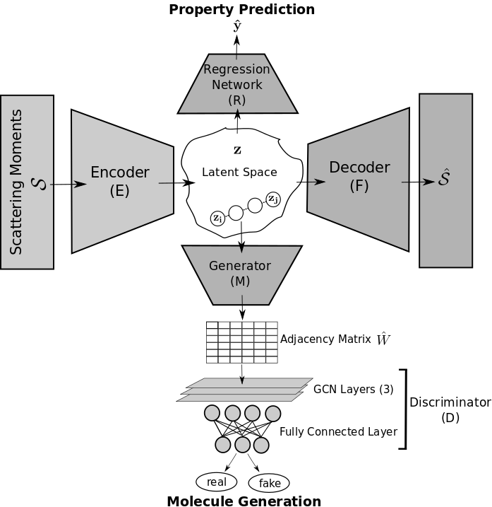
Figure 1: Overview of the GRASSY architecture including the 1) geometric scattering moments $\mathbf{S}$ computed on the input graph, passed to an 2) encoder network $E$ whose latent space is regularized for property prediction and for graph generation and trained for reconstruction via the 3) decoder $D$, and the 4) Molecular generation network trained with GAN and interpolation losses.

4.2 Learned scattering moments

Our proposed GRASSY framework uses the graph scattering transform to initially find a high dimensional embedding of the data. For each node-labelled molecular graph, we collect a set of signals associated with each label $\mathbf{x}_{L_{1}},\mathbf{x}_{L_{2}},\ldots\mathbf{x}_{L_{\ell}}$. Specifically, we define $\mathbf{x}_{L_{i}}(v_{j})=1$ if the vertex $v_{j}$ has label $L_{i}$ and $\mathbf{x}_{L_{i}}(v_{j})=0$ otherwise. We then perform multiscale wavelet transforms on each of these signals using a learnable scattering framework (Tong et al., 2021), and collect statistical moments by summing over the vertices (see Eqns. 3 and 4). We let $\mathbf{S}=\mathbf{S}(G)$ denote the collection of all scattering moments associated to a graph $G$ and use these moments as the input into the regularized autoencoder described below. Importantly, we note that while collecting these statistical moments, we apply a global summation and therefore the dimension of the the scattering embedding does not depend on the size of the graph.

4.3 Autoencoder Design

We feed the scattering moments $\mathbf{S}$ into a regularized autoencoder $F(E(X))$, which is penalized by two losses:

• The reconstruction loss that penalizes for errors in the reconstruction of scattering moments, i.e., $\mathcal{L}_{r}=\|\mathbf{S}-F(E(\mathbf{S}))\|$, where $E$ is the encoder and $F$ is the decoder.

• A regression loss which penalizes the failure of a property prediction network $R$ to predict a physicochemical properties $p$ of a given molecule from its latent representation, i.e., $\mathcal{L}_{p}=\|p-R(E(\mathbf{S}))\|$.

Note that $E(\mathbf{S}(G))$ is our proposed mapping function $f$ that approximates properties described in the problem setup. The molecule generation network, $M$, which we describe in the following subsection, is our proposed pseudo-inversion $f^{\prime}$ in the problem setup.

4.4 Molecule Generation

If $\mathbf{S}(G_{i})$ and $\mathbf{S}(G_{j})$ are the scattering moments corresponding to two graphs in our data set, we let $z_{i}=E(\mathbf{S}(G_{i}))$ and $z_{j}=E(\mathbf{S}(G_{i}))$ and consider the trajectory $z_{i\to j}(\alpha)\coloneqq(1-\alpha)z_{i}+\alpha z_{j}$. We let $M$ be a multi-layer perceptron which inputs scattering coefficients and outputs an $n\times n$ adjacency matrix and define $\hat{W}_{i\to j}(\alpha)\coloneqq M(z_{i\to j}(\alpha))$. As alluded to earlier, we wish to consider graphs of different sizes, and therefore we will take $n$ to be the size of the largest graph in the data set. Smaller adjacency matrices will be extended to be $n\times n$ via zero padding.

Inspired by the Autoencoder Adversarial Interpolation approach applied to images in Oring et al. (2020), we train $M$ and our discriminator $D$ using three losses adapted to the graph generation setting:

• The adjacency matrix reconstruction loss, $\mathcal{L}_{m}=\|W_{i}^{\text{pad}}-\hat{W}_{i}\|_{F}+\|W_{j}^{\text{pad}}-\hat{W}_{j}\|_{F}$, where adjacency matrices $W_{i}$ and $W_{j}$ are padded with zero vectors up to size $n\times n$.

• An adversarial loss, $\mathcal{L}_{a}=\sum_{k=0}^{K}-\log(D(\hat{W}_{i\to j}(k/K)))$, where discriminator, $D$, is a graph convolution network (GCN) that outputs a scalar value.

• A smoothness loss, $\mathcal{L}_{s}=\sum_{k=0}^{K}\left\lVert\frac{\partial\hat{\mathbf{S}}_{i\to j}(k/K)}{\partial\alpha}\right\rVert^{2}$, calculated by taking derivative of scattering moments produced by the decoder, $\hat{\mathbf{S}}_{i\to j}(\alpha)=F(z_{i\to j}(\alpha))$.

These losses aid in the production of valid molecular adjacency matrices which have similar structure to nearby points.

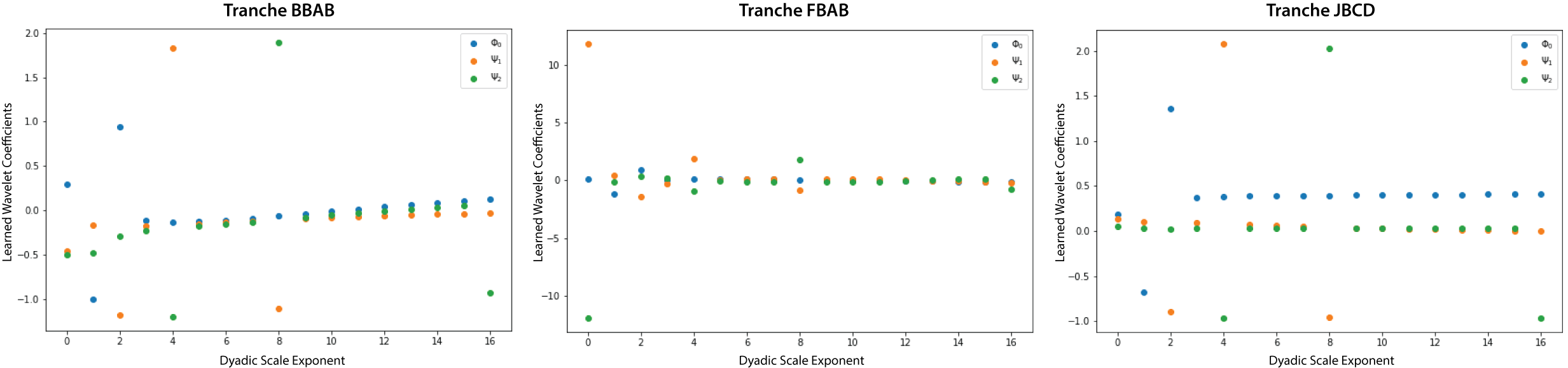
Figure 2: Learned geometric scattering wavelet coefficients for 3 ZINC tranches.

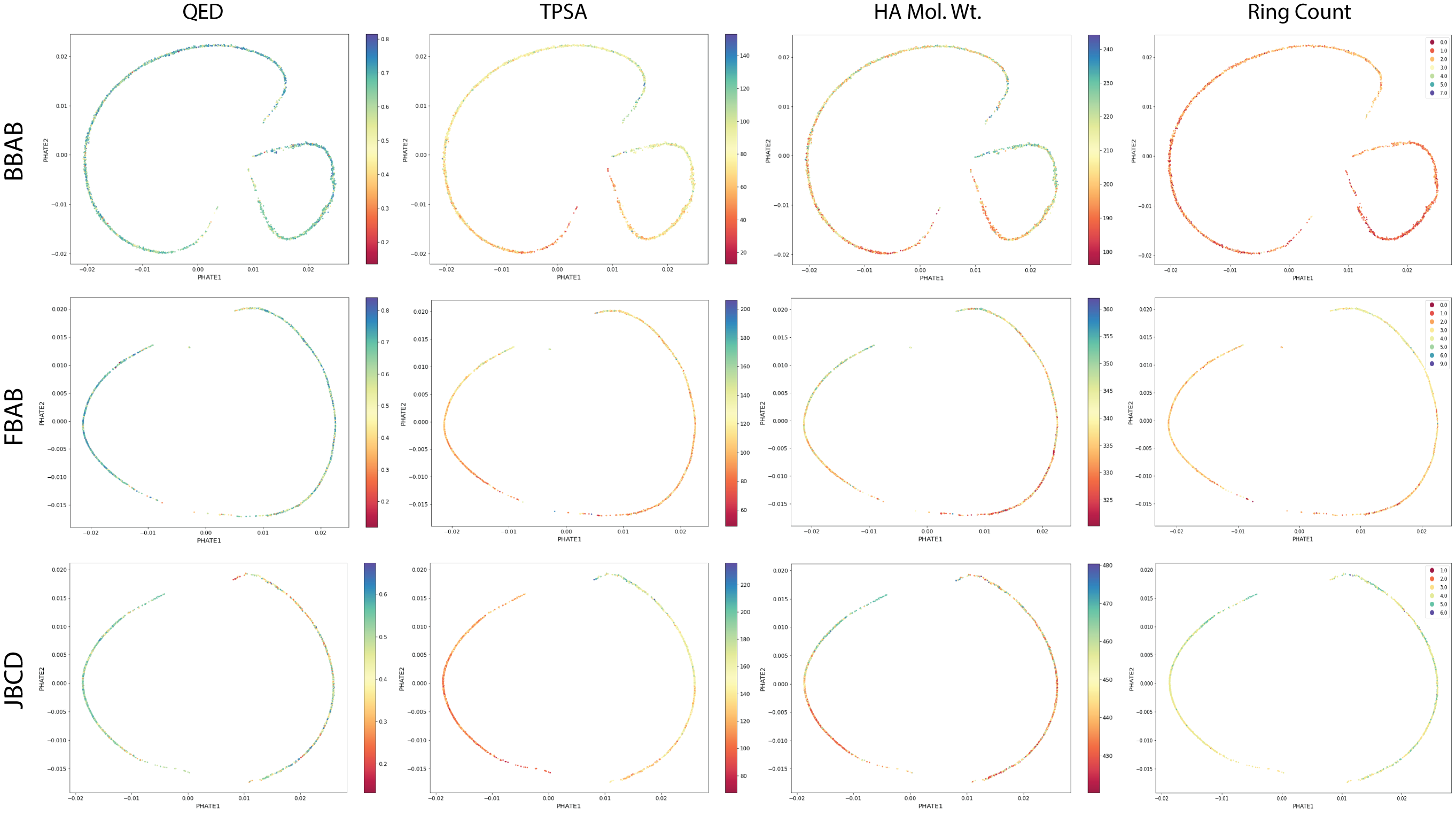
Figure 3: Latent representations of molecules in the ZINC dataset, visualized using PHATE, colored by value of physicochemical properties.

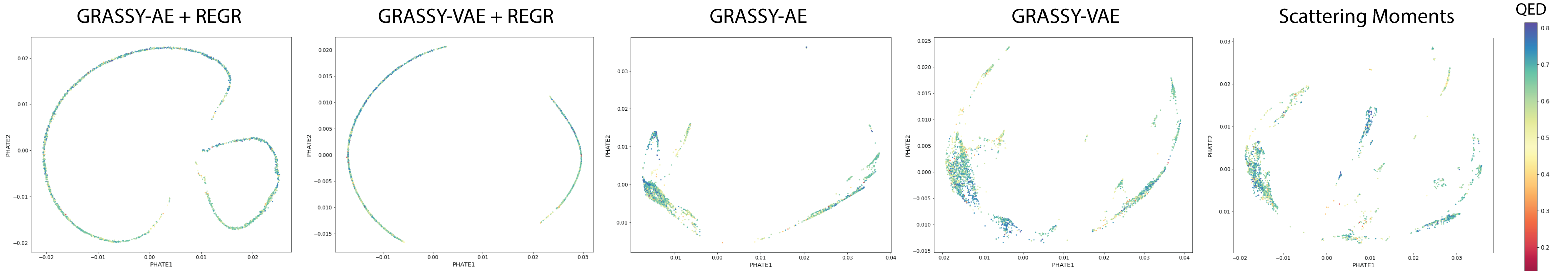
Figure 4: Latent representations obtained using ablations of the GRASSY model trained on the BBAB tranche of the ZINC dataset, color-coded by QED for different models.

Table 1: Molecular property prediction error

Model	Tranche	Molecular Properties
		QED	TPSA	Mol. Wt. (HA)	# Rings
	BBAB	$\mathbf{0.1677\pm 0.13}$	$\mathbf{13.20\pm 11}$	$\mathbf{22.83\pm 18}$	$\mathbf{0.6277\pm 0.52}$
GRASSY-AE + REGR	FBAB	0.2090 $\pm$ 0.16	17.15 $\pm$ 15	$\mathbf{32.89\pm 24}$	$\mathbf{0.7122\pm 0.57}$
	JBCD	$\mathbf{0.1941\pm 0.15}$	15.18 $\pm$ 12	$\mathbf{23.30\pm 22}$	$\mathbf{0.6604\pm 0.46}$
	BBAB	0.2063 $\pm$ 0.16	14.91 $\pm$ 13	56.67 $\pm$ 21	0.6302 $\pm$ 0.52
GRASSY-VAE + REGR	FBAB	$\mathbf{0.2041\pm 0.15}$	$\mathbf{16.94\pm 14}$	36.17 $\pm$ 23	0.7130 $\pm$ 0.54
	JBCD	0.2226 $\pm$ 0.17	$\mathbf{14.74\pm 12}$	34.54 $\pm$ 35	0.6643 $\pm$ 0.54
	BBAB	0.3947 $\pm$ 0.28	78.59 $\pm$ 20	210.0 $\pm$ 15	1.489 $\pm$ 0.92
GRASSY-AE	FBAB	1.401 $\pm$ 0.97	108.5 $\pm$ 22	340.4 $\pm$ 8.6	6.528 $\pm$ 1.1
	JBCD	0.4232 $\pm$ 0.26	126.9 $\pm$ 26	444.5 $\pm$ 14	3.152 $\pm$ 0.74
	BBAB	0.7413 $\pm$ 1.3	78.53 $\pm$ 20	209.4 $\pm$ 15	1.364 $\pm$ 0.93
GRASSY-VAE	FBAB	0.9313 $\pm$ 0.33	108.5 $\pm$ 22	339.5 $\pm$ 8.6	3.038 $\pm$ 0.96
	JBCD	2.885 $\pm$ 0.92	127.8 $\pm$ 26	444.7 $\pm$ 14	2.974 $\pm$ 0.86

Table 2: Smoothness of physicochemical properties in latent space

Model	Tranche	Molecular Properties
		QED	TPSA	Mol. Wt. (HA)	# Rings
	BBAB	0.0952	0.1716	0.0144	0.7153
GRASSY-AE + REGR	FBAB	0.1324	0.1353	0.0021	0.3172
	JBCD	0.1516	0.0645	0.0028	0.0928
	BBAB	0.0829	0.1785	0.0134	0.6415
GRASSY-VAE + REGR	FBAB	0.1298	0.1333	0.0020	0.3016
	JBCD	0.1225	0.0541	0.0031	0.0805
	BBAB	0.0692	0.1467	0.0138	0.6114
GRASSY-AE	FBAB	0.1203	0.1332	0.0023	0.3413
	JBCD	0.1383	0.0697	0.0037	0.0837
	BBAB	0.0696	0.1442	0.0147	0.6266
GRASSY-VAE	FBAB	0.1201	0.1423	0.0022	0.3593
	JBCD	0.1376	0.0713	0.0036	0.0800

Table 3: Fraction of graphs generated with molecule-like structure

ZINC	# Atoms		Validity	Models
Tranche	Min.	Max.	Threshold	GRASSY	GSAE	GraphAF	MolGAN ($\lambda=0$)
BBAB	8	18	5	0.86	0.22	0.79	0.32
FBAB	16	27	15	0.94	0.17	0.76	0.46
JBCD	28	36	25	0.73	0.09	0.54	0.41

5 Results

We trained GRASSY on large datasets of drugs and drug-like molecules from two databases, ZINC (Irwin and Shoichet, 2005) and BindingDB (Gilson et al., 2016). ZINC contains drug-like molecules organized into tranches by molecular weight (abbreviated mol. wt.), solubility (logP value), reactivity and commercial availability. BindingDB is a drug-target interaction (DTI) database, containing pairs of molecules and proteins with known binding affinity. We used three tranches from the ZINC database, namely FBAB, BBAB, and JBCD, which are organized by molecular weight. Molecules in BBAB range from 200 to 250 Daltons, molecules in FBAB range from 350 to 375 Daltons, and molecules from JBCD range from 450 to 500 Daltons. We sampled 2500 molecules from each tranche to use as training data and used the ChEMBL database (Davies et al., 2015) to obtain 10 physicochemical for each molecule. These properties include quantitative estimate of drug-likeliness (QED) introduced in Bickerton et al. (2012), total polar surface area (TPSA), general chemical descriptors (mol. wt. and heavy atom mol. wt.), topochemical descriptors (BalabanJ, BertzCT, HallKierAlpha), and Lipinski parameters (number of hydrogen bond donors, number of hydrogen bond acceptors, and ring count). We also trained on known inhibitors of two protein targets on BindingDB, henceforth referred to by their UniProtKB identifiers. These targets are P14416, a D(2) dopamine receptor, and P00918, Carbonic anhydrase 2. All BindingDB results are shown in the Appendix.

To calculate the scattering moments for an individual molecular graph, we labeled each node by atom type and used the signals $\mathbf{x}_{L_{1}},\ldots,\mathbf{x}_{L_{\ell}}$ as described in Section 4.1. We set the number of moments $Q=2$ and the number of scales $J=4$. Since our tranches ranged in molecular weight, we decided to use a learnable version of graph scattering proposed in Tong et al. (2021) to individually learn diffusion scales for each tranche rather than just using dyadic powers $2^{j}$. The learned wavelet coefficients for each of the three ZINC tranches can be seen in Figure 2. We then passed the scattering moments into our autoencoder, which applied regression penalties with respect to 10 physicochemical properties in latent space.

We adjusted the learning rates so that our network was properly able to learn the input data on each tranche, and we used an early stopping mechanism that monitored the validation loss to prevent the models from over-fitting our data. Figure 3 shows the latent space representations of each tranche trained on GRASSY, where the latent space is colored by four different properties, each of which was part of the latent space regression task.

We compare GRASSY to three state-of-the art frameworks for molecular graph generation: GraphAF (Shi et al., 2020), MolGAN (Cao and Kipf, 2018) and GSAE (Castro et al., 2020). For GraphAF, we trained the TorchDrug implementation using a custom dataloader but without any architectural modifications. For MolGAN, we set the hyperparameter $\lambda$ to $0$ (full RL version). We also compared with experimented with ablations of the GRASSY architecture, turning off and on the regression penalty (with or without REG), as well as toggling variational vs vanilla autoencoder training (GRASSY-VAE vs. GRASSY-AE).

We tested these GRASSY variations according to three criteria:

• Accuracy of physicochemical prediction in latent space across each of these models, measuring by absolute error. (See Tables 1 and 4.)

• Smoothness of the physicochemical properties in latent space, which we calculated from the graph Laplacian, $L$, of the diffusion potential graph obtained from the PHATE transform of the latent space embeddings. We calculated smoothness by $s\coloneqq\frac{p^{T}Lp}{p^{T}p}$, where $p$ is a vector containing properties of the points embedded. (See Tables 2 and 5)

• Fraction of valid molecules generated. (See Table 3)

Tables 2 and 5 show smoothness, as described above, of physicochemical properties in the latent space of various versions of our architecture. We have made bold values representing the highest smoothness in the latent space for each tranch (or protein target for BindingDB) trained on each property, across the various architectures. We can see that there is no version of our architecture that significantly outperforms the others across the board. Though, in general, the Figure 4 shows that each version of the GRASSY produces a smooth latent space with respect to the physicochemical properties listed.

Tables 1 and 4 show the molecular property prediction errors across different versions of our architecture on four different physicochemical properties. On both tables, we made bold the lowest error values for each property, across the various versions of GRASSY. Table 1 shows the prediction error across the three different tranches of ZINC we trained, BBAB, FBAB, and JBCD. We can see that GRASSY-AE + REGR significantly outperforms the other three versions of our architecture with respect to property prediction in the latent space on this dataset. Table 4 shows that GRASSY-VAE + REGR outperformed our other architectures when trained on the BindingDB data, across protein targets P14416 and P00918.

Molecule-like graphs were created by thresholding the adjacency matrix output of the generator of GRASSY and identifying the largest connected component. The resulting molecule was considered valid if it satisfied the following criteria:

• Number of vertices in the graph must exceed a “validity threshold", set according to size of molecules in the training tranche. Specifically, single atoms, diatomic and tri-atomic molecules are unlikely to function as drugs or inhibit the activity of any protein target.

• Any cycles/rings must not contain more than 10 vertices/atoms. In practice, most drugs contain 5 or fewer rings (Aldeghi et al., 2014).

• No vertex should have degree (covalent bonds) exceeding 5. Our data predominantly contains hydrogen, carbon, nitrogen, oxygen, sulphur, chlorine and fluorine atoms, none of which have enough valence electrons to bond with more than 5 atoms simultaneously.

Table 3 shows the fraction of valid molecules generated by GRASSY, GSAE (Castro et al., 2020), GraphAF (Shi et al., 2020) and MolGAN (full RL version with hyperparameter $\lambda=0$ (Cao and Kipf, 2018), according to the criteria above. The minimum and maximum number of atoms in the training molecules are listed to justify the choice of the validity threshold used to mark small generated molecules as invalid.

6 Conclusions

We have introduced GRASSY, a novel method for molecule generation. Given a dataset of molecules represented as graphs, we first collect a sequence of scattering moments for each graph. We then train a regularized autoencoder on these scattering moments to produce a latent representation which respects the physicochemical properties of each molecule. Finally, we produce new molecules by interpolating in latent space an applying a GAN which is trained to produce chemically valid molecules. In our experiments, we see that our network produces a higher proportion of realistic molecules than other methods. We also see that physicochemical properties of the molecules vary smoothly in our latent space and therefore that our network can be used to predict such properties.

Appendix A Appendix

Figures and tables associated with the BindingDB dataset are included below:

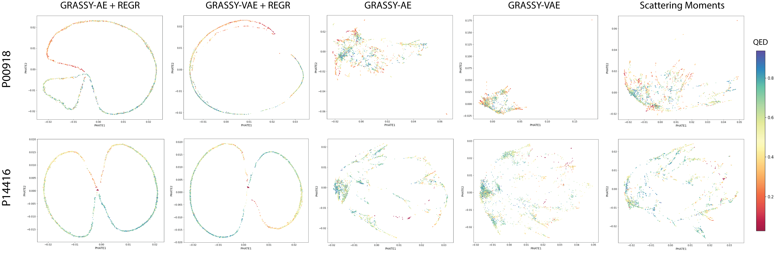
Figure 5: Latent representations obtained using ablations of the GRASSY model trained on the BindingDB dataset, color-coded by QED.

Table 4: Accuracy of physicochemical property prediction for BindingDB

Model	Protein	Molecular Properties
	Target	QED	TPSA	Mol. Wt. (HA)	# Rings
GRASSY-AE + REGR	P14416	0.3072 $\pm$ 0.43	22.52 $\pm$ 30	$\mathbf{49.51\pm 66}$	$\mathbf{0.8053\pm 1.6}$
	P00918	$\mathbf{0.2911\pm 0.22}$	35.50 $\pm$ 34	62.91 $\pm$ 71	0.8908 $\pm$ 0.75
GRASSY-VAE + REGR	P14416	$\mathbf{0.2430\pm 0.20}$	$\mathbf{18.99\pm 31}$	52.02 $\pm$ 66	0.9096 $\pm$ 1.9
	P00918	0.3395 $\pm$ 0.27	$\mathbf{34.80\pm 33}$	$\mathbf{56.72\pm 64}$	$\mathbf{0.7981\pm 0.66}$
GRASSY-AE	P14416	0.5672 $\pm$ 0.83	56.90 $\pm$ 74	399.1 $\pm$ 196	3.533 $\pm$ 1.4
	P00918	0.6871 $\pm$ 0.63	116.8 $\pm$ 57	373.3 $\pm$ 151	2.483 $\pm$ 1.5
GRASSY-VAE	P14416	0.7300 $\pm$ 0.35	56.86 $\pm$ 74	399.7 $\pm$ 197	4.154 $\pm$ 1.3
	P00918	0.6001 $\pm$ 0.30	117.1 $\pm$ 57	372.3 $\pm$ 150	2.630 $\pm$ 1.4

Table 5: Smoothness of physicochemical properties in latent space for BindingDB

Model	Protein	Molecular Properties
	Target	QED	TPSA	Mol. Wt. (HA)	# Rings
GRASSY-AE + REGR	P14416	0.1846	0.2813	0.0822	0.1494
	P00918	0.3786	0.4469	0.1611	0.5016
GRASSY-VAE + REGR	P14416	0.1746	0.3032	0.0716	0.1475
	P00918	0.3345	0.3991	0.1294	0.3926
GRASSY-AE	P14416	0.1811	0.2385	0.0995	0.1505
	P00918	0.2405	0.2436	0.1496	0.2954
GRASSY-VAE	P14416	0.2282	0.2688	0.1148	0.1818
	P00918	0.3685	0.4035	0.2368	0.4820

References

- Abu-El-Haija et al. [2019] Sami Abu-El-Haija, Bryan Perozzi, Amol Kapoor, Nazanin Alipourfard, Kristina Lerman, Hrayr Harutyunyan, Greg Ver Steeg, and Aram Galstyan. Mixhop: Higher-order graph convolutional architectures via sparsified neighborhood mixing. In international conference on machine learning, pages 21–29. PMLR, 2019.
- Yun et al. [2019] Seongjun Yun, Minbyul Jeong, Raehyun Kim, Jaewoo Kang, and Hyunwoo J Kim. Graph transformer networks. Advances in Neural Information Processing Systems, 32:11983–11993, 2019.
- Mallat [2012] Stéphane Mallat. Group invariant scattering. Communications on Pure and Applied Mathematics, 65(10):1331–1398, 2012.
- Shi et al. [2020] Chence Shi, Minkai Xu, Zhaocheng Zhu, Weinan Zhang, Ming Zhang, and Jian Tang. GraphAF: a Flow-based Autoregressive Model for Molecular Graph Generation. arXiv:2001.09382 [cs, stat], February 2020. URL http://arxiv.org/abs/2001.09382. arXiv: 2001.09382.
- Cao and Kipf [2018] Nicola De Cao and Thomas Kipf. MolGAN: An implicit generative model for small molecular graphs. CoRR, abs/1805.11973, 2018. URL http://arxiv.org/abs/1805.11973.
- Kipf and Welling [2017] Thomas N. Kipf and Max Welling. Semi-Supervised Classification with Graph Convolutional Networks. arXiv:1609.02907 [cs, stat], February 2017. URL http://arxiv.org/abs/1609.02907. arXiv: 1609.02907.
- Fan and Huang [2021] Shuangfei Fan and Bert Huang. Labeled Graph Generative Adversarial Networks. arXiv:1906.03220 [cs, stat], February 2021. URL http://arxiv.org/abs/1906.03220. arXiv: 1906.03220.
- Gómez-Bombarelli et al. [2018] Rafael Gómez-Bombarelli, Jennifer N. Wei, David Duvenaud, José Miguel Hernández-Lobato, Benjamín Sánchez-Lengeling, Dennis Sheberla, Jorge Aguilera-Iparraguirre, Timothy D. Hirzel, Ryan P. Adams, and Alán Aspuru-Guzik. Automatic Chemical Design Using a Data-Driven Continuous Representation of Molecules. ACS Central Science, 4(2):268–276, February 2018. ISSN 2374-7943, 2374-7951. doi:10.1021/acscentsci.7b00572. URL https://pubs.acs.org/doi/10.1021/acscentsci.7b00572.
- Coifman and Maggioni [2006] Ronald R. Coifman and Mauro Maggioni. Diffusion wavelets. Applied and Computational Harmonic Analysis, 21(1):53–94, July 2006. ISSN 1063-5203. doi:10.1016/j.acha.2006.04.004. URL https://www.sciencedirect.com/science/article/pii/S106352030600056X.
- Coifman and Lafon [2006] Ronald R. Coifman and Stéphane Lafon. Diffusion maps. Applied and Computational Harmonic Analysis, 21(1):5–30, 2006. ISSN 1063-5203. doi:https://doi.org/10.1016/j.acha.2006.04.006. URL https://www.sciencedirect.com/science/article/pii/S1063520306000546. Special Issue: Diffusion Maps and Wavelets.
- Moon et al. [2019] Kevin R. Moon, David van Dijk, Zheng Wang, Scott Gigante, Daniel B. Burkhardt, William S. Chen, Kristina Yim, Antonia van den Elzen, Matthew J. Hirn, Ronald R. Coifman, Natalia B. Ivanova, Guy Wolf, and Smita Krishnaswamy. Visualizing structure and transitions in high-dimensional biological data. Nature Biotechnology, 37(12):1482–1492, December 2019.
- van Dijk et al. [2017] David van Dijk, Juozas Nainys, Roshan Sharma, Pooja Kaithail, Ambrose J Carr, Kevin R Moon, Linas Mazutis, Guy Wolf, Smita Krishnaswamy, and Dana Pe’er. Magic: A diffusion-based imputation method reveals gene-gene interactions in single-cell rna-sequencing data. BioRxiv, page 111591, 2017.
- Haghverdi et al. [2016] Laleh Haghverdi, Maren Büttner, F Alexander Wolf, Florian Buettner, and Fabian J Theis. Diffusion pseudotime robustly reconstructs lineage branching. Nature methods, 13(10):845, 2016.
- Zou and Lerman [2020] Dongmian Zou and Gilad Lerman. Graph convolutional neural networks via scattering. Applied and Computational Harmonic Analysis, 49(3):1046–1074, 2020.
- Gama et al. [2018] Fernando Gama, Alejandro Ribeiro, and Joan Bruna. Diffusion scattering transforms on graphs. arXiv preprint arXiv:1806.08829, 2018.
- Gao et al. [2019] Feng Gao, Guy Wolf, and Matthew Hirn. Geometric scattering for graph data analysis. In Kamalika Chaudhuri and Ruslan Salakhutdinov, editors, Proceedings of the 36th International Conference on Machine Learning, volume 97 of Proceedings of Machine Learning Research, pages 2122–2131. PMLR, 09–15 Jun 2019. URL https://proceedings.mlr.press/v97/gao19e.html.
- Perlmutter et al. [2019] Michael Perlmutter, Feng Gao, Guy Wolf, and Matthew Hirn. Understanding Graph Neural Networks with Asymmetric Geometric Scattering Transforms. arXiv:1911.06253 [cs, stat], November 2019. URL http://arxiv.org/abs/1911.06253. arXiv: 1911.06253.
- Gama et al. [2019] Fernando Gama, Alejandro Ribeiro, and Joan Bruna. Stability of graph scattering transforms. Advances in Neural Information Processing Systems, 32:8038–8048, 2019.
- Min et al. [2020] Yimeng Min, Frederik Wenkel, and Guy Wolf. Scattering GCN: Overcoming oversmoothness in graph convolutional networks. arXiv preprint arXiv:2003.08414, 2020.
- Min et al. [2021] Yimeng Min, Frederik Wenkel, and Guy Wolf. Geometric scattering attention networks. In ICASSP 2021-2021 IEEE International Conference on Acoustics, Speech and Signal Processing (ICASSP), pages 8518–8522. IEEE, 2021.
- Tong et al. [2021] Alexander Tong, Frederik Wenkel, Kincaid MacDonald, Smita Krishnaswamy, and Guy Wolf. Data-Driven Learning of Geometric Scattering Networks. arXiv:2010.02415 [cs, stat], February 2021. URL http://arxiv.org/abs/2010.02415. arXiv: 2010.02415.
- Zou and Lerman [2019] Dongmian Zou and Gilad Lerman. Encoding robust representation for graph generation. In 2019 International Joint Conference on Neural Networks (IJCNN), pages 1–9. IEEE, 2019.
- Castro et al. [2020] Egbert Castro, Andrew Benz, Alexander Tong, Guy Wolf, and Smita Krishnaswamy. Uncovering the folding landscape of RNA secondary structure using deep graph embeddings. In 2020 IEEE International Conference on Big Data (Big Data), pages 4519–4528, 2020. doi:10.1109/BigData50022.2020.9378305.
- Oring et al. [2020] Alon Oring, Zohar Yakhini, and Yacov Hel-Or. Autoencoder Image Interpolation by Shaping the Latent Space. arXiv:2008.01487 [cs, stat], October 2020. URL http://arxiv.org/abs/2008.01487. arXiv: 2008.01487.
- Irwin and Shoichet [2005] John J. Irwin and Brian K. Shoichet. ZINC – A Free Database of Commercially Available Compounds for Virtual Screening. Journal of chemical information and modeling, 45(1):177–182, 2005. ISSN 1549-9596. doi:10.1021/ci049714. URL https://www.ncbi.nlm.nih.gov/pmc/articles/PMC1360656/.
- Gilson et al. [2016] Michael K. Gilson, Tiqing Liu, Michael Baitaluk, George Nicola, Linda Hwang, and Jenny Chong. BindingDB in 2015: A public database for medicinal chemistry, computational chemistry and systems pharmacology. Nucleic Acids Research, 44(D1):D1045–1053, January 2016. ISSN 1362-4962. doi:10.1093/nar/gkv1072.
- Davies et al. [2015] Mark Davies, Michał Nowotka, George Papadatos, Nathan Dedman, Anna Gaulton, Francis Atkinson, Louisa Bellis, and John P. Overington. ChEMBL web services: streamlining access to drug discovery data and utilities. Nucleic Acids Research, 43(W1):W612–W620, July 2015. ISSN 0305-1048. doi:10.1093/nar/gkv352. URL https://doi.org/10.1093/nar/gkv352.
- Bickerton et al. [2012] G. Richard Bickerton, Gaia V. Paolini, Jérémy Besnard, Sorel Muresan, and Andrew L. Hopkins. Quantifying the chemical beauty of drugs. Nature Chemistry, 4(2):90–98, February 2012. ISSN 1755-4349. doi:10.1038/nchem.1243. URL https://www.nature.com/articles/nchem.1243.
- Aldeghi et al. [2014] Matteo Aldeghi, Shipra Malhotra, David L Selwood, and Ah Wing Edith Chan. Two- and Three-dimensional Rings in Drugs. Chemical Biology & Drug Design, 83(4):450–461, January 2014. ISSN 1747-0277. doi:10.1111/cbdd.12260. URL https://www.ncbi.nlm.nih.gov/pmc/articles/PMC4233953/.