The Spitzer/IRAC Legacy over the GOODS Fields: Full-Depth $3.6$, $4.5$, $5.8$ and $8.0$ $\mu$m Mosaics and Photometry for $>9000$ Galaxies at $z\sim 3.5-10$ from the GOODS Re-ionization Era wide-Area Treasury from Spitzer (GREATS)

Abstract

We present the deepest Spitzer/IRAC $3.6$, $4.5$, $5.8$ and $8.0$ $\mu$m wide-area mosaics yet over the GOODS-N and GOODS-S fields as part of the GOODS Re-ionization Era wide-Area Treasury from Spitzer (GREATS) project. We reduced and mosaicked in a self-consistent way observations taken by the 11 different Spitzer/IRAC programs over the two GOODS fields from 12 years of Spitzer cryogenic and warm mission data. The cumulative depth in the $3.6$ $\mu$m and $4.5$ $\mu$m bands amounts to $\sim 4260$ hr, $\sim 1220$ hr of which are new very deep observations from the GREATS program itself. In the deepest area, the full-depth mosaics reach $\gtrsim 200$ hr over an area of $\sim 100$ arcmin², corresponding to a sensitivity of $\sim 29$ AB magnitude at $3.6$ $\mu$m ($1\sigma$ for point sources). Archival cryogenic $5.8$ $\mu$m and $8.0$ $\mu$m band data (a cumulative 976 hr) are also included in the release. The mosaics are projected onto the tangential plane of CANDELS/GOODS at a $0\farcs 3$ pixel^-1 scale. This paper describes the methodology enabling, and the characteristics of, the public release of the mosaic science images, the corresponding coverage maps in the four IRAC bands and the empirical Point-Spread Functions (PSFs). These PSFs enable mitigation of the source blending effects by taking into account the complex position-dependent variation in the IRAC images. The GREATS data products are in the Infrared Science Archive (IRSA). We also release the deblended $3.6$-to-$8.0$ $\mu$m photometry $9192$ Lyman-Break galaxies at $z\sim 3.5-10$. GREATS will be the deepest mid-infrared imaging until JWST and, as such, constitutes a major resource for characterising early galaxy assembly.

1 Introduction

Table 1: Summary of Spitzer/IRAC datasets included in the GREATS mosaics

Program name	PID	PI	Year	Max cov.	#	Total cov.	# frames	SSC Pipeline	Ref.
					point.			version
				[hr]		[hr]
GOODS-N
GOODS	$169$	Dickinson	$2004-2005$	$92.8$	$8$	$278.3$	$5364$	S18.25.0	[1]
SEDS	$61040$	Fazio	$2010-2011$	$12.6$	$33$	$179.1$	$6947$	S18.18.0/S19.1.0	[2]
S-CANDELS	$80215$	Fazio	$2012$	$25.3$	$4$	$101.2$	$3944$	S19.1.0	[5]
GREATS	$11134$	Labbé	$2015-2016$	$122.6$	$4$	$372.6$	$14628$	S19.1.0 /S19.2.0	[6]
	Totals:			$288.9$	$49$	$931.2$	$30833$
GOODS-S
GOODS	$194$	Dickinson	$2004$	$46.9$	$8$	$180.7$	$3494$	S18.25.0	[1]
UDF2	$30866$	Bouwens	$2006-2007$	$26.9$	$1$	$29.1$	$1098$	S18.25.0	[3]
SEDS	$60022$	Fazio	$2010-2011$	$8.8$	$54$	$211.8$	$8146$	S18.18.0/S19.0.0	[2]
IUDF	$70145$	Labbé	$2010-2011$	$103.0$	$4$	$215.6$	$8464$	S18.18.0/S19.0.0	[4]
ERS	$70204$	Fazio	$2011$	$95.6$	$2$	$163.0$	$6356$	S18.18.0
S-CANDELS	$80217$	Fazio	$2011-2012$	$25.3$	$4$	$101.2$	$3944$	S19.0.0 /S19.1.0	[5]
IGOODS	$10076$	Oesch	$2014$	$45.5$	$2$	$65.6$	$2576$	S19.1.0	[4]
GREATS	$11134$	Labbé	$2015-2016$	$71.8$	$4$	$234.3$	$9200$	S19.1.0 /S19.2.0	[6]
	Totals:			$315.8$	$79$	$1201.3$	$43278$

Note. — Programs PID 81 and PID 20708 were omitted because they only contribute $0.14$ hr and $0.5$ hr depth per pixel and per band, respectively, over the central parts of the GOODS-S region.

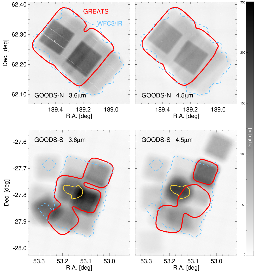
Figure 1: The inverted grey-scale images present the coverage maps, in units of hours, in the $3.6$ $\mu$m (left) and $4.5$ $\mu$m band (right) for the GOODS-N and GOODS-S fields (top and bottom row, respectively) from all IRAC programs prior to GREATS. The red contours mark the coverage provided by the GREATS program, while the light blue dashed contour corresponds to the footprint of the stacked CANDELS/3D-HST WFC3/IR F125W-, F140W- and F160W-band mosaics. The yellow contours displayed for GOODS-S correspond to the small ($\lesssim 10$ arcmin²) region with a depth $\geq 150$ hr in both bands prior to GREATS. The same grey scale is adopted for all the images to illustrate the depth as indicated by the vertical bar on the right, in units of hours.

During the last $\sim 20$ years, the two fields of the Great Observatories Origins Deep Survey initiative (GOODS-N and GOODS-S - Giavalisco et al. 2004) have accumulated an impressive array of observations ranging from the X-rays to the radio. In particular, the improvements in sensitivity and resolution provided by the Hubble Space Telescope (HST) Wide Field Camera 3 (WFC3 - Kimble et al. 2008) in 2009 fostered the acquisition of exquisitely deep optical and near-infrared (NIR) data over these fields through programs such as the Cosmic Assembly Near-infrared Deep Extragalactic Legacy Survey (CANDELS - Grogin et al. 2011; Koekemoer et al. 2011), 3D-HST (van Dokkum et al. 2011; Brammer et al. 2012) and the Hubble Ultra/Extreme Deep Field campaigns (UDF09/UDF12/XDF - Oesch et al. 2010; Bouwens et al. 2010; Ellis et al. 2013; Illingworth et al. 2013).

These observations have enabled the identification of $\sim 400$ plausible galaxies at $z>8$ (e.g., Bouwens et al. 2015; Finkelstein et al. 2015), probing epochs as early as $z\sim 10-12$ (e.g., Oesch et al. 2010, 2013, 2016, 2018; Bouwens et al. 2011, 2013, 2014, 2019; Ellis et al. 2013 - but see also Coe et al. 2013; Zitrin et al. 2014; Calvi et al. 2016; McLeod et al. 2016; Salmon et al. 2018; Livermore et al. 2018; Morishita et al. 2018; Salmon et al. 2020 for similar searches over different fields).

At $z\gtrsim 4$ HST/WFC3 observations only probe the rest-frame ultraviolet (UV). The Spitzer InfraRed Array Camera (IRAC - Fazio et al. 2004) provided a crucial extension into the rest-frame optical at $4\lesssim z\lesssim 10$, key for studying the stellar mass assembly (e.g. Duncan et al. 2014; Grazian et al. 2015; Song et al. 2016; Stefanon et al. 2017a; Davidzon et al. 2018), and nebular line emission (e.g., Labbé et al. 2013; Smit et al. 2014; Faisst et al. 2016; De Barros et al. 2019) at early cosmic epochs.

Obtaining coverage of the GOODS fields with Spitzer had already been recognized as a priority for the first year of its operations (Giavalisco et al. 2004). Indeed, during its 5 years 9 months of cryogenic mission and the following $10$ years $8$ months of warm observations (with an end-of-mission on January 30th, 2020), the GOODS fields have been targeted with IRAC by a dozen major programs (see Table 1), totaling $\sim 3$ months of observations per IRAC band.

In this paper we present full-depth mosaics in the IRAC $3.6$, $4.5$, $5.8$ and $8.0$ $\mu$m bands which combine all relevant observations over the GOODS-N and GOODS-S fields. Specifically, in this release we include new observations at $3.6$ and $4.5$ $\mu$m from the GOODS Re-ionization Era wide-Area Treasury from Spitzer program (GREATS - PI: I. Labbé). All the observations were processed using the latest calibrations and combined together into final mosaics using the same procedure as we earlier pioneered in Labbé et al. (2015). These procedures resulted in a consistent set of data products similar to those produced in that earlier study (see also Damen et al. 2011 for further details). Thanks to its superb depth, this dataset constitutes a natural extension at $3-8$ $\mu$m of the Hubble Legacy Field initiative (HLF - Illingworth et al. 2016; Whitaker et al. 2019; Illingworth et al. 2021 in prep.). We also release the photometry in the four IRAC bands, obtained after removing the contamination from neighbours, for $9192$ candidate Lyman-Break galaxies at $z\sim 3.5-10$ identified by Bouwens et al. (2015) over the GOODS-N and GOODS-S fields.

This paper is organized as follows. In Section 2 we describe the strategy of the observations. Section 3 summarizes the main steps involved in the reduction of the observations, mosaic and PSF creation. In Section 4 we present the main features of the mosaics, in Section 5 we describe the procedure we followed to extract the photometry from the GREATS mosaics, while in Section 6 we briefly highlight several science cases motivating the GREATS program. In Section 7 we specify the data products made available to the community, with the conclusions in Section 8.

Table 2: Summary of GREATS AORs

Field	AOR	R.A.	Dec.	Pos. Angle	MJD
Name		[degrees]	[degrees]	[degrees]	[days]
GOODS-N	$54396672$	$189.2613220$	$62.1838341$	$145.60$	$57242.3203125$
	$54396416$	$189.2128754$	$62.1937408$	$145.46$	$57242.4375000$
	$54396160$	$189.2434082$	$62.1968384$	$145.39$	$57242.5507812$
	$54395904$	$189.2602844$	$62.1841393$	$145.31$	$57242.6679688$
GOODS-S	$54319616$	$53.1282692$	$-27.8142986$	$69.03$	$57140.3789062$
	$54318848$	$53.0915413$	$-27.8234711$	$69.13$	$57140.4921875$
	$54316032$	$53.1064072$	$-27.8310547$	$69.20$	$57140.6093750$
	$54317056$	$53.1110954$	$-27.8082600$	$69.56$	$57141.1210938$

Note. — This Table only presents data for the first four AORs in each field. The full list of AORs is available online. The execution time of each AOR is $\sim 2.75$h, with a frame time of $100$s and exposure time of $93.6$s per frame. Each GOODS-N AOR covers an area of $\sim 50$arcmin² per band, while each GOODS-S AOR covers $\sim 25$arcmin² per band.

2 Data

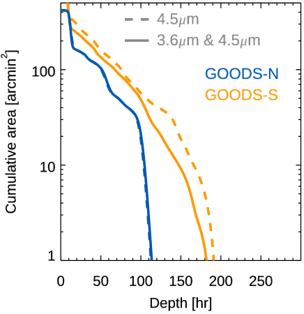
Figure 2: Cumulative area as a function of coverage depth (in hours) for the $4.5$ $\mu$m band (which has the shallowest coverage of the two bands) for the mosaic combining all observations prior to adding in the GREATS compared to the cumulative area where $3.6$ and $4.5$ $\mu$m bands simultaneously benefit from the same minimum coverage depth (dashed and solid curves, respectively), for the GOODS-N and GOODS-S fields (blue and orange curve, respectively).

The GOODS fields are centered at $\alpha=$12^h36^m55^s, $\delta=$+62°14^′15^′′ (GOODS-N) and $\alpha=$03^h32^m30^s, $\delta=$-27°48^′20^′′ (GOODS-S), respectively, and benefit from extensive IRAC coverage. Specifically, our mosaics combine essentially all observations from past programs to new observations at $3.6$ $\mu$m and $4.5$ $\mu$m from the GREATS program (PI: I. Labbé). The main properties of the programs included in our analysis are summarized in Table 1.

2.1 Archival coverage

The GOODS-N field was observed for $558.6$ hr in the $3.6$ and $4.5$ $\mu$m each and for $278.3$ hr in each of the $5.8$ and $8.0$ $\mu$m bands, while GOODS-S was observed for $967.0$ hr in each of the $3.6$ and $4.5$ $\mu$m bands and $209.8$ hr at $5.8$ and $8.0$ $\mu$m, for a total of $4027.4$h. Observations in the $5.8$ and $8.0$ $\mu$m bands were feasible only during the cryogenic part of the mission, making the accumulation of data in these channels significantly shorter than is available in the $3.6$ and $4.5$ $\mu$m bands.

2.2 GREATS observing strategy and coverage

Our Cycle 11 GREATS program added significantly to the GOODS archival datasets, primarily by adding the crucial deep data needed for a number of wide-ranging science investigations. GREATS contributed $606.9$ hr of additional coverage in each of the $3.6$ and $4.5$ $\mu$m bands, bringing the cumulative coverage in each of these bands to $\sim 2132.5$ hr, and in the four bands to $5241.2$ hr.

Consistent photometric depth across multiple wavelength channels is key for obtaining detailed probes of the spectral energy distribution (SED) of high redshift galaxies (Labbé et al. 2015). Unfortunately, the different observational programs over the GOODS fields led to rather heterogeneous datasets, resulting in very position-dependent IRAC depths. GOODS-S suffered more clearly from this issue: ultradeep ($\gtrsim 150$ hr) coverage existed in both the $3.6$ and $4.5$ $\mu$m bands; yet, only a tiny $\sim 10$ arcmin² area was observed at this depth in both bands, limiting the scientific value of the dataset. This can qualitatively be seen in Figure 1, and, more quantitatively, in Figure 2.

The main aim of the GREATS program was to significantly extend the ultradeep $\sim 150$ hr coverage to $\gtrsim 150$ arcmin² across both GOODS fields, while at the same time improving the overall homogeneity of the $3.6$ and $4.5$ $\mu$m band coverage. The layout of the observations was carefully chosen to complement and expand the already existing data, taking advantage of the change in position angle of the arrays as Spitzer travelled along its orbit, maximizing the survey efficiency. The full set of Astronomical Observation Requests (AORs) from the GREATS program are listed in Table 2. Observations over the GOODS-N field were split into two pointings executed $\sim 180$ days apart, with each pointing covering the rectangular area of two contiguous arrays. To gain more uniform depth in the GOODS-S field required us to organize the observations into four pointings, each one probing the region corresponding to one array. All AORs were executed with a medium cycling dithering pattern. The resulting additional coverage is shown in Figure 1.

3 Data reduction and mosaic creation

To limit systematics and to generate uniformly-processed mosaics, we downloaded from the Spitzer Heritage Archive all the relevant observations from all the programs overlapping the CANDELS GOODS footprint. The full dataset consists of 845 AORs (392 + 453, for GOODS-N and GOODS-S, respectively), for a total of 168234 individual frames (72494 in GOODS-N and 95740 in GOODS-S, respectively).

The data reduction started with the most recent corrected Basic Calibrated Data (cBCD) generated by the Spitzer Science Center (SSC) calibration pipeline. This subtracts the dark frames, homogenizes the pixel response (detector linearization and flat fielding), corrects for known artifacts (column pull up/down, muxbleed, first frame effect), and provides per-frame uncertainty estimates, bad pixel mask, and cosmic ray rejection masks.

We post-processed the cBCD frames following the same custom pipeline used by Labbé et al. (2015). This pipeline improves on these initial corrections and masks (see Sec. 3.1 of Labbé et al. 2015), combines the frames and generates the final mosaics. In the following Section we summarize the pipeline’s main steps, referring the reader to Damen et al. (2011) and Labbé et al. (2015) for further details.

3.1 IRAC reduction process

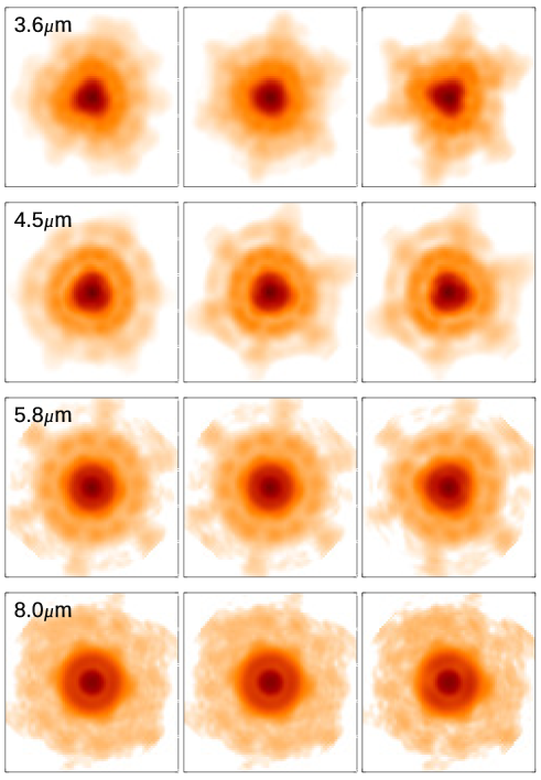
Figure 3: Examples of point-spread functions (displayed with a logarithmic intensity map) at different positions across the GOODS-N field. Each row refers to a specific IRAC band, as indicated by the label at the top-left corner of the left-most panel. In each row, the three panels, $\sim 24^{\prime\prime}$-wide, show PSFs in the GOODS-N field at same declination, but spaced in R.A. by $\sim 15^{\prime}$. They highlight the rapid spatial variation of the PSFs across the IRAC field, particularly evident for the $3.6$ and $4.5$ $\mu$m bands. A similar variation is seen in GOODS-S. Such dramatic variations clearly complicate the analysis and the photometry.

In general, cBCDs from different programs were generated using different SSC pipeline versions (see Table 1). The main differences consist of astrometry, image distortion refinements, and artifact correction. These issues were all handled directly in our own reduction pipeline, and hence these updates by the SSC have no effect on our end products. We note here that the flux density calibration has not changed significantly since S18.8, and therefore our mosaics use the latest flux calibrations consistent with S19.2.

The reduction with our custom pipeline is based on a two-pass procedure, where each AOR was reduced independently. The first pass included the following steps: an initial removal of background and bias structure from each frame estimated from the median of all the frames in the AOR; correction of column pull-up and pull-down introduced by bright stars or cosmic rays subtracting a median above and below the affected pixels after excluding any sources; persistence masking and muxbleed correction rejecting all highly exposed pixels in the subsequent $4$ frames.

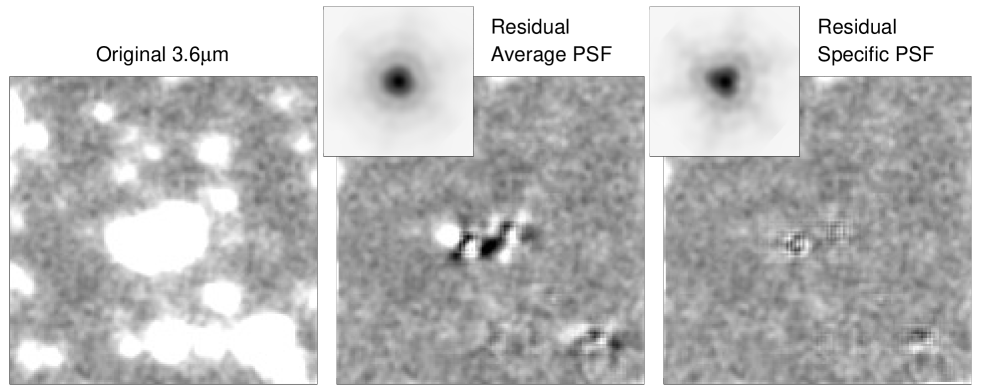
Figure 4: Impact of the PSF construction method on prior-based photometry. The panel on the left shows an image stamp at a random location in the GREATS GOODS-N $3.6$ $\mu$m science mosaic. The middle and right panels present two different residuals after subtracting from the science image a model built convolving the 3D-HST detection image (Skelton et al., 2014) with a convolution kernel based on the PSF in the $3.6$ $\mu$m band displayed in the inset at the corresponding top-left corner (using a logarithmic stretch and inverted grey scale). The central panel shows the residual from subtracting the average PSF over the full GOODS-N field (comparable to the PSF built by stacking isolated point sources across the field), while the panel on the right shows the residual using our position-dependent PSF, as pioneered by Labbé et al. (2015). All image stamps are $27\farcs 5$ per side. The position-dependent PSF minimizes systematics in the photometry, and clearly produces superior photometric results.

The second pass included cosmic ray rejection, astrometric calibration and an accurate large-scale background removal. Cosmic ray hits were cleaned through iterative sigma clipping. The astrometry was corrected applying a rigid shift in both R.A. and Dec. estimated from sources in common with the deep maps of CANDELS/3D-HST (Skelton et al., 2014). The absolute astrometric reference of CANDELS/GOODS-N was registered to the Sloan Digital Sky Survey, the Two Micron All Sky Survey (2MASS), and the deep Very Large Array (VLA) $20$ cm survey (Morrison et al. 2010), while that for CANDELS/GOODS-S was anchored to the $R$-band mosaic from the ESO Imaging Survey (EIS - Arnouts et al. 2001), registered to the Guide Star Catalog II (GSC-II - Lasker et al. 2008 - Koekemoer et al. 2011). The background level was first estimated as the median of the frames in each AOR masking sources and outlier pixels, and refined by iteratively clipping pixels belonging to objects and subtracting the mode of the background pixels. The frames were then drizzled (Fruchter & Hook, 2002) using a pixfrac = $0.4$ on a common reference grid defined by the CANDELS tangent point and a fine $0\farcs 3$ pixel^-1 scale, to allow for easy re-binning onto commonly adopted pixel scales. The individual drizzled AORs were combined into the final mosaic after weighting each pixel according to its depth.

The output pixels in the final drizzled image are not independent of each other, causing the pixel-to-pixel noise in the output image to be correlated. The correlation implies that direct estimates of the pixel-to-pixel noise in the drizzled output image underestimates the noise on large scales. For the drizzle parameters used here, an approximate correction from the single-pixel noise to the noise at large scales can be derived following Casertano et al. (2000). At an output pixel scale of $0\farcs 3$ (scale $=0.25$ relative to the $1\farcs 2$ input pixel) each (pixfrac$=0.4$) drizzled input pixel contributes to $1.6$ output pixels. In this case, the noise at large scales is a factor $2.0$ higher than estimated from the pixel-to-pixel rms (see Casertano et al. 2000 Appendix A6 for pixfrac $>$ scale). An output image at a scale of $0\farcs 6$ can easily be produced from the $0\farcs 3$ scale images by simply block summing the science images and weight maps by a factor $2$ in each dimension. The resulting image at $0\farcs 6$ scale has drizzle pixfrac $=0.4$ and scale $=0.5$, so each drizzled pixel contributes to $<1$ output pixel. In this case, the noise over large areas is a factor $1.36$ higher than estimated from the pixel-to-pixel noise.

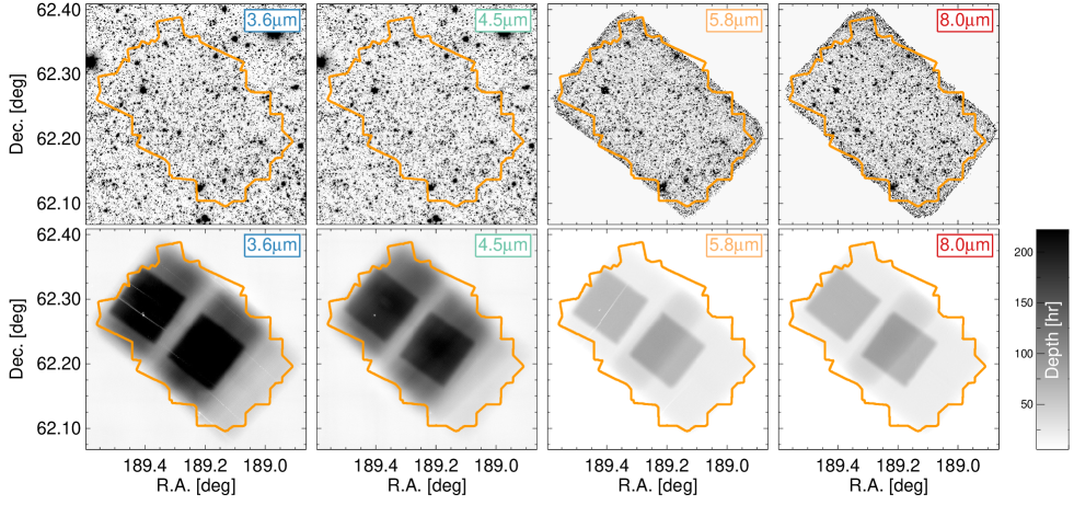
Figure 5: Full GREATS mosaics in the IRAC $3.6$, $4.5$, $5.8$ and $8.0$ $\mu$m bands (left to right, respectively) for the CANDELS/GOODS-N field. The top row presents the science mosaics in inverted grey scale, while the bottom row shows the coverage maps, with the effective depth indicated by the vertical bar on the right. The orange contour in each panel corresponds to the region covered by the 3D-HST detection mosaic (Skelton et al., 2014), combining the data in the HST/WFC3 F125W, F140W and F160W bands. The coverage in the $3.6$ and $4.5$ $\mu$m beyond the CANDELS boundary is provided by the SEDS program.

3.2 Point-spread function creation

The instrumental point-spread function (PSF) in the IRAC bands, particularly in the $3.6$ and $4.5$ $\mu$m bands, shows a peculiar, approximately triangular shape (see. e.g., the Spitzer Space Telescope Observer Manual - Sect. 6.1.2.2). AOR observations spread over periods of time of the order of months cause observations of the same patch of the sky to have position angles differing by tens of degrees. These angular offsets result from a change in the spacecraft roll angle of approximately $1$ deg per day. The combination of the instrumental PSF at different position angles results in complex light profiles for the final PSFs, which can also change rapidly over small spatial scales. Accurate reconstruction of the PSF, then, becomes an essential step to obtain robust IRAC photometry using either PSF- or prior-based fitting techniques. However, identifying a suitable number of high-S/N isolated point sources at different locations across the field is generally a challenging task in deep extragalactic fields due to source crowding.

Figure 6: Full GREATS mosaics in the IRAC $3.6$, $4.5$, $5.8$ and $8.0$ $\mu$m bands (left to right, respectively) for the CANDELS/GOODS-S field. The top row presents the science mosaics in inverted grey scale, while the bottom row shows the coverage maps, with the effective depth indicated by the vertical bar on the right. The orange contour in each panel corresponds to the region covered by the 3D-HST detection mosaic (Skelton et al., 2014), combining the data in the HST/WFC3 F125W, F140W and F160W bands. The coverage in the $3.6$ and $4.5$ $\mu$m beyond the CANDELS boundary is provided by the SEDS program.

To overcome this problem, we leveraged the remarkable instrumental stability of IRAC over its life cycle. We created extremely high S/N empirical PSFs in the four IRAC bands stacking several hundred observations of bright, unsaturated point sources (see Labbé et al. 2015 for full details), and we adopted these as a template. These templates extend to a radius of $12\farcs 0$ and share the pixel scale of the science mosaics ($0\farcs 3$/pixel - see Section 4); location-dependent PSFs were then generated combining the template by rotating and stacking according to the position angles and coverage depth of each AOR stored in a fine grid (steps of $12\farcs 0$) of locations across each mosaic.

Our PSF reconstruction procedure takes advantage of the approximate invariance of the effective PSF of the IRAC array across its field of view (FoV). Comparison between $3\farcs 0$-diameter aperture photometry from the warm mission on the $100\times$-oversampled IRAC Point Response Function (PRF - IRAC Instrument Handbook) at the edges of the IRAC FoV to that from the PRF at the center of the array resulted in systematic differences of $\lesssim 3\%$. Most importantly, the GREATS mosaics combine, at each point on the sky, observations from different programs. These sampled the same patch of sky at different portions of the IRAC array, averaging over the effective PSF of all contributing exposures. The end result is a finely sampled PSF at each location in the GOODS fields.

In Figure 3 we present examples of the PSF variation in the $3.6$ $\mu$m band. These examples highlight the dramatic changes in the shape of the PSF even across small regions of the mosaics. They indicate that the adoption of non-optimal PSFs in prior-based photometry may introduce systematic effects. We further illustrate this in Figure 4. The strong variation of the PSF profile across the mosaics makes the adoption of the average PSF much less effective at correctly reproducing the observed light profiles of the objects. The resulting residuals are substantial and can introduce systematic errors in the flux density estimates. The adoption of the optimal PSF results in marginal residuals (see also e.g., Figure 4 of Merlin et al. 2016). As an aide to future photometric studies, we release together with our mosaics, the template PSF with the AOR mapping data and a Python script to reconstruct the PSF at arbitrary locations across the mosaics.

4 Results

4.1 Mosaic properties

The final full-depth IRAC mosaics in the four bands, together with the corresponding coverage maps, are shown in Figure 5 and 6 for the GOODS-N and GOODS-S fields, respectively. Color images combining $K_{\mathrm{S}}$-band, $3.6$ and $4.5$ $\mu$m are shown in Figures 7 and 8 for GOODS-N and GOODS-S, respectively.

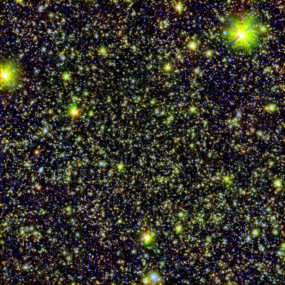
Figure 7: Color composite image of the GOODS-N field ($\sim 20^{\prime}\times 20^{\prime}$) obtained combining the new Spitzer/IRAC imaging from the GREATS program (red and green respectively show the IRAC $4.5$ and $3.6$ $\mu$m emission) with the $K_{\mathrm{s}}$ data (shown in blue) from the MODS (Kajisawa et al. 2011) and CFHT $K_{\mathrm{s}}$ (Wang et al., 2010) programs.

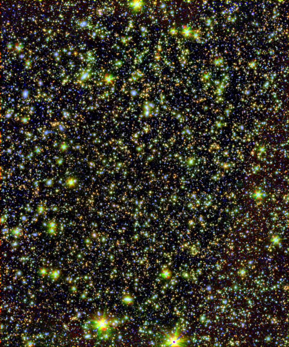
Figure 8: Color composite image of the GOODS-S field ($\sim 23^{\prime}\times 28^{\prime}$) obtained combining the new Spitzer/IRAC imaging from the GREATS program (red and green respectively show the IRAC $4.5$ and $3.6$ $\mu$m emission) with the $K_{\mathrm{s}}$ data (shown in blue) from the TENIS (Hsieh et al. 2012) and HUGS (Fontana et al. 2014) programs.

The FWHMs of the PSFs, measured from their radial profile, and their $1$ $\sigma$ dispersions across the field are $1\farcs 52\pm 0\farcs 02$ at $3.6$ $\mu$m for both fields; $1\farcs 49\pm 0\farcs 02$ and $1\farcs 50\pm 0\farcs 02$ at $4.5$ $\mu$m (GOODS-N and GOODS-S, respectively); $1\farcs 72\pm 0\farcs 01$ and $1\farcs 69\pm 0\farcs 01$ at $5.8$ $\mu$m (GOODS-N and GOODS-S, respectively); and $2\farcs 06\pm 0\farcs 01$ and $2\farcs 04\pm 0\farcs 01$ at $8.0$ $\mu$m (GOODS-N and GOODS-S, respectively). These value indicate excellent and constant image quality across the two fields; the FWHMs for the two bluer bands are consistent at $\lesssim 2\sigma$ with those of the IUDF program (Labbé et al., 2015).

The photometric calibration was verified using $\sim 80$ bright ($m\lesssim 21$ AB) unsaturated point sources spread across each field. We measured their flux densities in large ($6\farcs 0$ radius) apertures and find excellent agreement ($<2\%$) with measurements from the S-CANDELS mosaics (Ashby et al., 2015). Comparison to the original GOODS mosaics revealed a larger offset, $\sim 8\%$ in the $3.6$ $\mu$m band and $\lesssim 2\%$ in the $4.5$ $\mu$m band for both fields, consistent with Labbé et al. (2015). These offset are understood and are due to the different flux calibration of the BCD pipeline used to reduce the original GOODS observations (see Labbé et al. 2015 for details). Based on these comparisons, we estimate the accuracy of our flux density maps to be $2\%$.

4.2 Astrometric reference

The registration to the reference CANDELS frame is accurate to $<0\farcs 0045$ with a $1$ $\sigma$ dispersion of $0\farcs 077$. Comparison of the astrometry between the CANDELS/3D-HST GOODS mosaics and the second release of the Gaia catalogue (Gaia DR2 - Gaia Collaboration et al. 2018; Lindegren et al. 2018) showed that in each field the astrometric reference suffered from position-dependent distortions with offsets of $\sim 0\farcs 08$ rms (Illingworth et al. 2021 in prep.). Furthermore, the astrometry of GOODS-S is affected by an overall shift of $\sim 0\farcs 3$ to the North and $\sim 0\farcs 1$ to the West, consistent with what found by Rujopakarn et al. (2016) for the HUDF. Given the offsets to the Gaia DR2 astrometric reference are marginal compared with the PSF FWHMs, we ultimately opted not to apply any further correction to the GREATS astrometric solution. The released GREATS mosaics therefore share the same astrometric reference as CANDELS.

We anticipate that the extraction of information from the GREATS mosaics will be performed in one of the following two ways, ultimately depending on whether the sources of interest have a counterpart in a high-resolution image. If a counterpart is available, its IRAC photometry would be best measured with one of the tools developed for prior-based photometry (e.g., Tfit - Laidler et al. 2007, and descendants) and adopting as prior a mosaic with the same astrometric reference of GREATS (such as those from CANDELS or 3D-HST). Nonetheless, because current tools for prior-based photometry can accommodate small position-dependent shifts ($\sim 0\farcs 2-0\farcs 4$), we expect only marginal systematic effects in photometry even when adopting as prior high-resolution mosaics whose astrometric reference is consistent with that of Gaia. The detailed impact of these effects would however depend on the geometry of the individual sources and on the alignment capabilities of the tools adopted for the photometry. Broadly, however, the spatial coordinates of the objects of interest can then be anchored to the Gaia astrometric reference by registering to the coordinates of the object on the high-resolution image. The astrometric accuracy for sources without a high-resolution counterpart will be subject to the $0\farcs 08$ scatter discussed above (natively or after applying a rigid offset of (R.A., Dec.) $=(0\farcs 1,-0\farcs 3)$ for the GOODS-N and GOODS-S mosaics, respectively). However, we would note for any investigations involving direct detection of sources on the IRAC mosaics, that the source positional uncertainties will be dominated by the broad IRAC PSF, likely requiring pre-imaging for follow-up observations where $\sim$few$\times$ mas accuracy is necessary (e.g., as for JWST/NIRSpec - Bagnasco et al. 2007; JWST User Documentation 2016-).

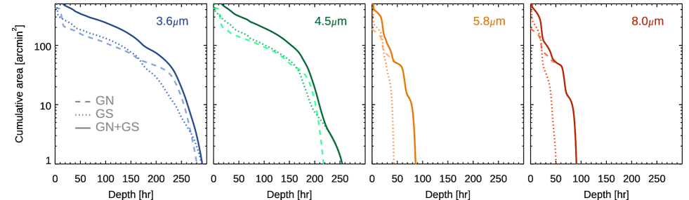
Figure 9: Cumulative area as a function of the depth (in hours) for the final GREATS mosaics in the $3.6$, $4.5$, $5.8$ and $8.0$ $\mu$m bands, respectively, as indicated by the label at the top-right corner. In each panel, the different curves correspond to the area for the CANDELS/GOODS-N, CANDELS/GOODS-S and their combination, according to the legend in the left panel.

4.3 Coverage Depth

In Figure 9 we present the cumulative area as a function of the coverage depth for the four bands, for the individual fields and when combined together. Overall, the two fields have approximately the same coverage depth distribution in the $3.6$ and $4.5$ $\mu$m bands, $\sim 3-5\times$ deeper than the $5.8$ and $8.0$ $\mu$m bands. Furthermore, the $5.8$ and $8.0$ $\mu$m coverage in GOODS-N is generally $\sim 2\times$ deeper than in GOODS-S.

The coverage of the $3.6$ $\mu$m band reaches a maximum depth of $\sim 250$ hr over $\sim 5-10$ arcmin² in each field, while that of the $4.5$ $\mu$m band reaches $\sim 200$ hr over $\sim 10-20$ arcmin² area in each field. Remarkably, the mosaics in the $3.6$ $\mu$m ($4.5$ $\mu$m) band provide an ultradeep coverage of at least $150$ hr ($120$ hr) over a cumulative area of $\sim 150$ arcmin² ($\sim 1/2$ the total area of the CANDELS footprint of the GOODS fields).

The full-depth coverage maps presented in Figure 5 and 6 qualitatively show that for both GOODS fields the coverage depth with the $3.6$ $\mu$m band is spatially distributed in a very similar way across the mosaic as that in the $4.5$ $\mu$m band. This is presented more quantitatively in Figure 10. The substantial overlap between the cumulative area in the $4.5$ $\mu$m band coverage with that of the minimum coverage between $3.6$ and $4.5$ $\mu$m bands indicates that, despite some inhomogeneities in the depth of coverage in each field, the per-pixel coverage in the $3.6$ $\mu$m band is at least as deep as that in the $4.5$ $\mu$m band over most of the GOODS area. Specifically, for GOODS-S, for $\sim 95\%$ of the area with $>75$ hr depth coverage, the coverage depth in the $3.6$ $\mu$m band is at least $90\%$ of that in the $4.5$ $\mu$m band. This is quite remarkable considering the initial coverage inhomogeneity discussed in Section 2.

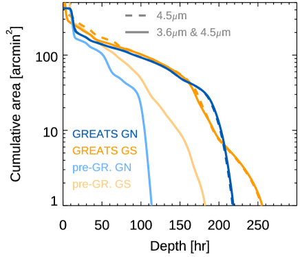
Figure 10: Cumulative area vs. per-pixel-depth (in hours) in the $4.5$ $\mu$m band (dashed curves) and vs. the minimum per-pixel-depth in the $3.6$ and $4.5$ $\mu$m bands (solid curves), for the GOODS-N and GOODS-S fields (blue and yellow, respectively). Darker colors refer to the GREATS mosaics, while lighter curves correspond to the cumulative areas for the mosaics combining all data available prior to GREATS. These are reproduced here from Figure 2 for comparison.

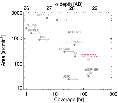
Figure 11: The GREATS coverage in the context of the major Spitzer/IRAC surveys for high-redshift galaxies. The horizontal axis at the top presents an approximate $1$ $\sigma$ depth in the $3.6$ $\mu$m band for point sources from the SENS-PET calculator (but see the discussion in Section 4.4). Data points refer to the following programs: IUDF (Labbé et al., 2015), UDF2 (Labbé et al., 2013), SIMPLE (Damen et al., 2011), Frontier Fields (FF; PI: Soifer - see e.g., Shipley et al. 2018), SPLASH (Steinhardt et al., 2014), SEDS (Ashby et al., 2013a), S-CANDELS (Ashby et al., 2015), SMUVS (Ashby et al., 2018), SpUDS (Caputi et al., 2011), EGS (Barmby et al., 2008), GOODS (PI: Dickinson) and IDF/NEP (Krick et al. 2009 - where the data point was extracted from the Data Release 2 mosaic)^a. Arrows identify those programs executed during cryogenic cycles, and indicate, by the end point of the arrow, that cryogenic observations were $\sim 2\times$ more efficient in the $3.6$ $\mu$m band than warm mission ones (SENS-PET). Building in part on existing observations, GREATS extends the depth of IUDF to an area $\sim 5\times$ larger.

^a http://spider.ipac.caltech.edu/staff/jason/darkfield/styled/index.html

Figure 11 shows the position of the GREATS full-depth mosaics in the depth-area plane (where we adopt the characteristic depth of $150$ hr over $150$ arcmin² in the $3.6$ $\mu$m band) and compares it to other significant extragalactic deep surveys executed with Spitzer. GREATS provides a depth comparable to that of IUDF but over a $\sim 5\times$ larger area.

4.4 Sensitivity

The nominal $1$ $\sigma$ limits for point sources in the $3.6$ and $4.5$ $\mu$m bands from the SENS-PET exposure time calculator that correspond to the maximum coverage depth in the GREATS mosaics ($250$ hr and $200$ hr, for the $3.6$ and $4.5$ $\mu$m band, respectively) are $9.1$ nJy ($29.0$ AB) and $14.7$ nJy ($28.5$ AB), respectively. The $150$ hr coverage (that we adopted in Section 4.3 as a typical depth of the GREATS mosaics) corresponds to $1$ $\sigma$ limits of $11.8$ nJy ($28.7$ AB) and $17.0$ nJy ($28.3$ AB) for the $3.6$ and $4.5$ $\mu$m bands, respectively. The available coverage in the $5.8$ and $8.0$ $\mu$m bands is shallower. In the GOODS-N field, the maximum coverage is $\sim 90$ hr, corresponding to $1$ $\sigma$ photometric limits of $141$ nJy ($26.0$ AB) and $172$ nJy ($25.8$ AB) for the $5.8$ and $8.0$ $\mu$m bands respectively. Meanwhile, the maximum depth over the GOODS-S field is $\sim 40$ hr, corresponding to $1$ $\sigma$ limits of $211$ nJy ($25.6$ AB) and $258$ nJy ($25.4$ AB) in the $5.8$ and $8.0$ $\mu$m mosaics, respectively.

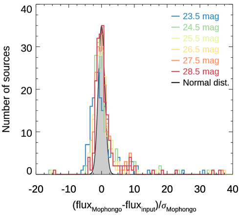
Figure 12: Distribution of the differences between the flux density of synthetic sources recovered by Mophongo (flux${}_{\mathrm{\textsc{Mophongo}}}$) and their nominal values (flux_input), in units of flux density uncertainty ($\sigma_{\mathrm{\textsc{Mophongo}}}$). The synthetic sources were injected at random locations within one of the regions of the $3.6$ $\mu$m GOODS-N mosaic with the deepest coverage. Each color corresponds to a specific value of the input flux density, indicated by the legend. The grey solid area with black outline corresponds to a Normal distribution with a peak value of $35$, approximately corresponding to the peak value of the histograms. Most of the measurements follow a Normal distribution with only a small fraction of sources deviating appreciably from it ($\lesssim 10\%$ of the sources have differences $>5$ $\sigma$). These results, (see also an earlier demonstration by Labbé et al. 2015), indicate that the source confusion effects in deep IRAC imaging can be reliably mitigated even in the faintest regimes.

However, the actual detection significance will depend on the impact of source confusion on the photometry for specific sources. For deep imaging with low resolution, as it is the case for the GREATS $3.6$ and $4.5$ $\mu$m mosaics, confusion from source blending may decrease the actual sensitivity. For an instrument with a resolution similar to IRAC, Franceschini et al. (1991) estimated the confusion limit to be $\sim 0.6-2$ $\mu$Jy (depending on whether the source is point-like or extended). According to the SENS-PET calculator, this limit is already exceeded in the shallowest regions of the GREATS mosaic. However, Franceschini et al. (1991) advanced the hypothesis, quantified by Labbé et al. (2015), that high-resolution imaging of the same patch of the sky can be used to effectively deblend the sources in the low-resolution image, enabling measurements down to fainter limits. Below we briefly summarize the results of Labbé et al. (2015).

Table 3: GREATS photometry for the LBGs of Bouwens et al. (2015)

ID	R.A.	Dec.	$z$ bin	$3.6$ $\mu$m	$4.5$ $\mu$m	$5.8$ $\mu$m	$8.0$ $\mu$m
	[hh:mm:ss.sss]	[dd:pp:ss.ss]		[nJy]	[nJy]	[nJy]	[nJy]
GNWB-7485214158	12:37:48.529	62:14:15.83	$4$	$112.7\pm 25.8$	$60.3\pm 30.8$	$-193.9\pm 252.9$	$330.1\pm 347.2$
GNWB-7502914551	12:37:50.292	62:14:55.12	$4$	$158.0\pm 31.5$	$125.2\pm 28.3$	$189.5\pm 265.1$	$-204.9\pm 330.7$
GNWB-7546714582	12:37:54.674	62:14:58.20	$4$	$215.6\pm 56.7$	$159.1\pm 55.8$	$291.7\pm 260.7$	$-254.5\pm 460.0$
GNWB-7485914550	12:37:48.598	62:14:55.07	$4$	$132.9\pm 26.9$	$102.4\pm 22.9$	$-312.4\pm 247.2$	$-107.2\pm 329.8$
GNWB-7575615181	12:37:57.561	62:15:18.16	$4$	$141.7\pm 102.4$	$98.7\pm 66.2$	$-59.1\pm 241.3$	$857.1\pm 357.5$

Note. — This Table only presents data for the first five sources. It is available in its entirety in machine-readable form.

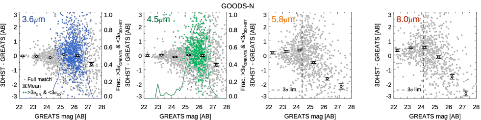
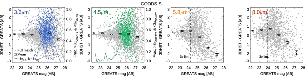
Figure 13: Comparison between the IRAC photometry extracted from the GREATS mosaics and that from the 3D-HST program (Skelton et al. 2014), for the matching LBG sample of Bouwens et al. (2015). The top row refers to sources in the GOODS-N field, while the bottom row to sources in GOODS-S. In each row, each panel corresponds to individual IRAC bands, as labelled in the top-left corners. In each panel, the grey filled circles mark the difference in magnitude of the matching sources between the two catalogs, while the black open circles with error bars the mean and the error on the mean. In the panels corresponding to the $3.6$ and $4.5$ $\mu$m measurements, the blue and green points mark those sources which have $\geq 3$ $\sigma$ significance in the GREATS data but $<3$ $\sigma$ in the 3D-HST catalogs, providing a first assessment of the gain in sensitivity enabled by GREATS. The solid curve corresponds to the fraction of such sources compared to the underlying population of LBGs, and it is referred to the vertical axis on the right. The dashed vertical line in the $5.8$ and $8.0$ $\mu$m panels marks an approximate $3$ $\sigma$ limit. No significant offsets exist with previous photometry. It is evident how GREATS mostly benefits sources around $26$ mag, corresponding to $\sim L^{*}$ at $z\sim 8$ (e.g., Stefanon et al. 2019).

Using prior-based photometry of synthetic zero-flux sources in the GOODS-S field, Labbé et al. (2015) studied the relation between the point-source sensitivity and integration time. The considered depths ranged from $\sim 30$ hr to $200$ hr, very similar to the range available for the GREATS mosaics. They found that the $1$ $\sigma$ limit of flux density decreases approximately as the nominal $1/\sqrt{t_{\mathrm{exp}}}$ expected for Poisson statistics (see their Equations 3 and 4 and their Figure 11 – the measured exponents are $-0.453$ and $-0.456$ for the $3.6$ and $4.5$ $\mu$m band, respectively, consistent with the Poissonian $-0.5$ exponent at a $2.5$ $\sigma$), and found no indication for any confusion limits or noise floor down to the deepest regions (Labbé et al. 2015). However, they found that limits in flux density were consistently $10\%-30\%$ shallower than the nominal values expected from SENS-PET for the same integration times (see Figure 11 of Labbé et al. 2015). These discrepancies could be the result of residual confusion from either sources below the detection limit in the high-resolution image or from extended wings of the surface brightness profile, that could still could contribute noise.

To further ascertain the impact of source confusion in the extraction of flux densities from deep IRAC images, we performed a Monte Carlo simulation, consisting of injecting synthetic point sources at random positions across a rectangular area of $\sim 4\farcm 1\times 2\farcm 5$ centered at [R.A., Dec.]=[$12$:$36$:$47$, $+62$:$13$:$08$] in the $3.6$ $\mu$m GOODS-N mosaic from GREATS. This region is characterized by $\sim 250$ hr-deep coverage, one of the deepest existing for IRAC. The choice of a point-like morphology is likely not significantly impacting our results due to the small sizes of faint high-redshift sources (e.g., Shibuya et al. 2015; Bouwens et al. 2021) and the broad IRAC PSFs.

Synthetic sources with the same intrinsic brightness were added at $20$ random positions. Their flux densities were successively extracted with Mophongo (Labbé et al. 2006, 2010b, 2010a, 2013, 2015). This tool leverages the brightness profile of each source from a high-resolution image to remove all neighbouring objects within a radius of $9\farcs 0$, before performing aperture photometry. Photometry was extracted adopting $1\farcs 8$-diameter apertures, and corrected to total using the brightness profile of each source on the low-resolution image and the PSF reconstructed at the specific locations of each source. These steps were executed for different values of intrinsic brightness (from $23.5$ mag to $28.5$ mag at constant intervals of $1$ mag). The full procedure was repeated $10$ times to improve the statistical significance. The results of this simulation are summarized in Figure 12, and show that the systematic effects from source confusion in the deep GREATS mosaics can be robustly accounted for.

In the present work, to facilitate the comparison with other surveys, all quoted flux density limits refer to the nominal values provided by the SENS-PET calculator. However, to provide a sense of the effect of source blending on the actual limits, we also present the $1$ $\sigma$ depths estimated with the relations of Labbé et al. (2015). We find that the deepest $250$ hr coverage in the $3.6$ $\mu$m band corresponds to $14.1$ nJy ($28.5$ AB), while the $200$ hr in the $4.5$ $\mu$m band corresponds to $17.6$ nJy ($28.3$ AB). Similarly, the $150$ hr coverage corresponds to $17.8$ nJy ($28.3$ AB) and $20.0$ nJy ($28.1$ AB) for the $3.6$ and $4.5$ $\mu$m bands, respectively.

5 IRAC Photometric catalog for $\sim 10000$ Lyman-Break galaxies in the GOODS fields

We also publicly release photometric information extracted from the GREATS mosaics for the Lyman-Break galaxy samples identified by Bouwens et al. (2015) in the GOODS-N and GOODS-S fields (including ERS, XDF, HUDF091 and HUDF092). This sample is composed by a total of $9192$ sources ($3914$ sources in GOODS-N, $5278$ in GOODS-S) initially selected to have redshifts $z\sim 3.5-10$ (see Bouwens et al. 2015 for details). This catalog was already adopted by the studies of De Barros et al. (2019) and Stefanon et al. (2021a, b). We remark here that the new, deeper IRAC data provided by the GREATS mosaics could lead to $z\lesssim 3-4$ solutions to be more likely for some of the sources in the catalog. We therefore advise the interested reader to perform a full SED analysis including both HST and IRAC photometry, if a more robust sample of LBGs is needed. Joint NIR-selected multi-wavelength catalogs incorporating the GREATS data will be released in a forthcoming paper.

Flux densities and uncertainties were extracted with Mophongo adopting a combination of WFC3 F125W-, F140W- and F160W-band mosaics as a high-resolution prior. Photometry was extracted adopting $1\farcs 8$-diameter apertures, and corrected to total using the brightness profile and the PSF curve of growth of each source.

Table 3 presents the first five entries of the photometric catalog, for reference. The full catalog is available online. In Figure 13, instead, we compare our new GREATS photometry to that of Skelton et al. (2014), who adopted the SEDS v1.2 data release (Ashby et al. 2013b) for the $3.6$ and $4.5$ $\mu$m bands, and the GOODS Spitzer release for the imaging at $5.8$ and $8.0$ $\mu$m. No significant offset is evident between the two sets of photometry, in particular in the $3.6$ and $4.5$ $\mu$m bands, where the new observations from the GREATS program were added. It is also remarkable the gain in S/N for $\sim 70-90\%$ of the sources around $\sim 26$ AB in these two bands. The marginal differences in the $5.8$ and $8.0$ $\mu$m band photometry likely result from the combined impact of an improved background subtraction, brightness profile modelling and PSF reconstruction implemented in the version of Mophongo adopted to extract the photometry from the GREATS data.

6 Key Science Enabled by GREATS

There has been a significant amount of progress in quantifying the properties of galaxies in the first few billion years of the universe (see e.g. Stark 2016). Nevertheless, a large number of open questions remain which require large area, deep IR datasets. There are important, contemporary science issues that can only be well-addressed by IR observations of greater sensitivity and over greater area. While JWST will ultimately provide such datasets, the GREATS mosaics provide opportunities to work with such IR data now. The purpose of this section is to present a few of the main science cases that will set the stage for advancing the field and providing focus for future JWST observations.

6.1 Stellar mass estimates at $z>7$

Characterizing the mass buildup of the first galaxies provides important constraints to galaxy formation models (e.g. Behroozi et al. 2013, 2019; Tacchella et al. 2018). A number of works have estimated the assembly of stellar mass ($M_{\star}$) with redshift down to the first $\sim 1$ Gyr of cosmic history ($z\gtrsim 6$ - e.g., González et al. 2014; Duncan et al. 2014; Grazian et al. 2015; Song et al. 2016; Stefanon et al. 2017a; Davidzon et al. 2017; Bhatawdekar et al. 2019; Kikuchihara et al. 2020). However, the area and sensitivity of the pre-GREATS IRAC coverage only allows individual detections of a handful of galaxies at $z\sim 8$, with similar numbers from stacking analysis. To robustly measure the stellar mass assembly at $z\sim 8-10$, significant samples of $z>8$ LBGs individually detected in IRAC bands are required. These large rest-frame optical samples can significantly reduce the impact of uncertainties in SFHs or dust content of galaxies relative to studies executed with only rest-frame UV data. The GREATS mosaics provide nominal $\geq 4$ $\sigma$ individual detections at $3.6$ $\mu$m for $\sim 50\%$ of the sources at $z\sim 8$ with $L\geq 0.4L^{*}$ over CANDELS GOODS-S and GOODS-N. As GREATS coverage only exists over $\sim 50\%$ of the CANDELS GOODS footprint, this is effectively equivalent to our detecting $100\%$ of the galaxies lying in areas with ultra-deep coverage from IRAC. This addresses the need for large samples, but the impact of dense fields on the sensitivity estimates (see the discussion in Sect. 4.4) needs to be kept in mind.

6.2 Nebular emission at $z>6$

There is increasing amount of evidence indicating that galaxies at $z\gtrsim 4$ are characterized by strong nebular emission at rest-frame optical, with equivalent width EW([O III]+$H\beta$) in excess of 800 Å  (Fumagalli et al. 2012; Stark et al. 2013; Smit et al. 2014, 2015; Faisst et al. 2016; Rasappu et al. 2016; Khostovan et al. 2016; Stefanon et al. 2017b, 2019; De Barros et al. 2019; Lam et al. 2019; Bowler et al. 2020). These fascinating results suggest that high-redshift galaxies likely have high specific SFR (sSFR$\gtrsim 10$ Gyr^-1) and young ages (few tens $\times$ Myr to few hundreds $\times$ Myr). Such impressive results have been obtained by characterizing the strong variations of the $[3.6]-[4.5]$ color with redshift. The flux changes seen reflect the contribution of the main emission lines (e.g., [O III], $H\beta$, $H\alpha$, [N II]) entering and leaving the $3.6$ and $4.5$ $\mu$m bands depending on the redshift (see e.g., Labbé et al. 2013; Smit et al. 2014; Faisst et al. 2016). The depth of IRAC observations prior to GREATS however limited the exploration for such lines in sources beyond $z\sim 6$. GREATS enables the investigations of the occurrence of such lines to finally be extended to $z>6$. Furthermore, recent studies have shown that the existence of strong rest-frame optical lines can substantially, and incorrectly, boost the estimates of stellar mass (e.g., Stark et al. 2013) if not accounted for. Therefore robust estimates of the emission line strength will also improve stellar mass estimates. GREATS has already been used to demonstrate the gains that will be made with this datatset. This can be seen in the recent paper by De Barros et al. (2019) where new [O III]+H$\beta$ measurements at $z\sim 8$ are made based on the GREATS IRAC $3.6$ and $4.5$ $\mu$m mosaics.

6.3 The rise of passive galaxies

A major uncertainty in current models of galaxy evolution is when and how passive galaxies start to appear in the Universe. There have already been some exciting selections of evolved, red galaxies identified at $z\sim 4-6$ (e.g., Guo et al. 2012; Caputi et al. 2012; Straatman et al. 2014; Stefanon et al. 2015), with a record-holder at $z\sim 9$ (Hashimoto et al. 2018). Only a handful of such passive galaxies are spectroscopically confirmed (Marsan et al. 2017; Glazebrook et al. 2017; Schreiber et al. 2018; Hashimoto et al. 2018; Forrest et al. 2020). Due to their red colors, such galaxies can remain completely undetected in current HST datasets, making IRAC the only instrument currently able to detect the most extreme sources. Due to the limited depth and area of current IRAC imaging, current searches for passive systems at $z>4$ have so far exclusively focused on the high-mass end ($M_{\star}\sim 10^{10.5-11}$ $M_{\odot}$). Ultradeep IRAC observations like those from GREATS will enable us to access lower stellar masses $M_{\star}\lesssim 10^{9.5-10}$ $M_{\odot}$ where the likelihood of finding such sources may increase.

6.4 SFR-$M_{\star}$ at $z>7$

A growing number of observations have identified a tight relation ($\sigma\lesssim 0.3$ dex - (Daddi et al. 2007; Whitaker et al. 2012; Schreiber et al. 2015; Kurczynski et al. 2016) between the SFR and $M_{\star}$ (the so-called main sequence of star-forming galaxies - Noeske et al. 2007) up to $z\sim 6-7$ (e.g., Labbé et al. 2010b; Bouwens et al. 2012; Stark et al. 2013; González et al. 2014; Duncan et al. 2014; Steinhardt et al. 2014; Salmon et al. 2015; Song et al. 2016; Jiang et al. 2016; Santini et al. 2017; Iyer et al. 2018; Pearson et al. 2018; Khusanova et al. 2020; Faisst et al. 2019). Indeed, a correlation between the SFR and $M_{\star}$ is predicted by models (e.g., Finlator et al. 2007, 2011, 2018; Dekel et al. 2009; Davé et al. 2011; Lu et al. 2014; Mancuso et al. 2016; Wilkins et al. 2017; Ma et al. 2018; Ceverino et al. 2018; Rosdahl et al. 2018; Tacchella et al. 2018). The scatter, slope and normalization constrain the SFH, feedback mechanisms and cold gas accretion. However, limitations in the estimates of stellar mass from current rest-frame UV-selected LBGs have only allowed a tentative determination of this relation at high redshifts ($z\sim 7$ - Labbé et al. 2010b). The samples have been further limited to the brightest sources. The lower stellar mass limits enabled by GREATS ($M_{\star}\sim 10^{9.5}$ $M_{\odot}$ for $z\lesssim 8-9$) will allow us to include $\sim 5\times$ more sources at $z>4$, and most importantly, with more robust stellar mass estimates.

7 Public Data Release

The data release accompanying this paper consists of the reduced images of all ultradeep IRAC observations over the GOODS-North and GOODS-South fields. We enhance this data release with flux density estimates in the four IRAC bands for all the Lyman-Break galaxies in the GOODS fields identified by Bouwens et al. (2015) at $z\sim 3.5-10$.

Specifically, this data release includes the following:

1. Science images and coverage maps in the $3.6$, $4.5$, $5.8$ and $8.0$ $\mu$m bands. Our reduction uses the same tangent point as CANDELS on pixel scales of $0\farcs 3$ pixel^-1, so the IRAC maps can be easily rebinned and registered to HST/WFC3 data.

2. Reduced images of all individual 845 AORs, drizzled onto the same grid, which may be useful to study the reliability or variability of sources.

3. Template PSFs and spatial maps of the weights and position angles of each AOR, allowing the reconstruction of the PSF at arbitrary locations. A python code to reconstruct the PSF at the desired location within the mosaic is also provided.

4. A catalog containing the position, flux density and uncertainty estimates in the four IRAC bands for the $9192$ sources identified by Bouwens et al. (2015) in the CANDELS/GOODS fields as candidate Lyman-Break galaxies consistent with redshifts in the range $z\sim 3.5-10$ (Bouwens et al. 2015).

These data products are publicly available through the IRSA website. The units of the science images are MJy/sr. Equivalently, flux densities can be obtained by multiplying the image pixel values by $2.1154\mu$ Jy DN^-1, corresponding to an image AB zeropoint of 23.0865 mag. Coverage maps are in units of seconds based on the warm mission observations; the higher sensitivity of the cryogenic observations is dealt with by scaling the cryogenic exposure times by a factor $1.7$.

8 Summary and Conclusions

Our mosaics include $\sim 610$ hr of new observations per band from the GOODS Re-ionization Era wide-Area Treasury from Spitzer (GREATS, PI: I. Labbé) program. Remarkably, these new GREATS observations enable a significant transformation of all the available data on GOODS-S and GOODS-N into a uniquely deep and wide imaging resource. The GREATS Mosaics are the result of combining $2132$ hr of observation in the $3.6$ and $4.5$ $\mu$m IRAC band, and $488$ hr in the $5.8$ and $8.0$ $\mu$m bands. GREATS data extend the ultradeep coverage in the $3.6$ and $4.5$ $\mu$m bands with $>150$ hr of deep data (corresponding to a $1$ $\sigma$ sensitivity for point sources of $\sim 12$ nJy in the $3.6$ $\mu$m band - SENS-PET) across $\sim 150$ arcmin² ($\sim 1/2$ the total area of the GOODS fields). This area is $5\times$ the area currently covered by the similarly-deep previous dataset IUDF (Labbé et al. 2015). The GREATS mosaics reach an impressive $250$ hr coverage in a small $\sim 5-10$ arcmin² region in each field in the $3.6$ and $4.5$ $\mu$m bands. Through accurate planning of the new GREATS observations, there is a good match between the depth in the $4.5$ $\mu$m coverage and the $3.6$ $\mu$m coverage over the two GOODS fields. Specifically, $\sim 95\%$ of the area in the GOODS fields with $>75$ hr depth in the $4.5$ $\mu$m band has $>90\%$ of that integration time in the $3.6$ $\mu$m band (best seen in Figure 10). The nominal sensitivity of the IRAC coverage is a close match to that available with WFC3/IR over the CANDELS Deep regions, enabling $\sim 4$ $\sigma$ detections for $\sim$half of the sample of $L>0.4L^{*}$ galaxies at $z\sim 8$. This allows for the characterization of optical emission lines and the much more reliable estimate of stellar masses for a substantial samples of galaxies at $z\sim 7-10$. Added knowledge of these aspects are important to fully prepare for science with JWST.

Our public release includes for each field and band the science mosaics and corresponding coverage maps. In addition, the release also includes PSF maps which take into account the complex spatial variation of the survey geometry. These PSF maps are an essential resource for optimally mitigating the impact of source blending. The science frames are calibrated to an AB zeropoint of $23.0865$mag, while the coverage maps have units of seconds and include a $1.7\times$ upscaling to account for the higher sensitivity achieved during the cryogenic mission. The mosaics are characterized by a quite uniform PSF FWHM$\sim 1\farcs 49-1\farcs 52$ at $3.6$ and $4.5$ $\mu$m ($\sim 1\farcs 7-2\farcs 0$ in the $5.8$ and $8.0$ $\mu$m bands, respectively) across the fields. The uniformity of the PSF FWHM provides consistent image quality. The mosaics have the tangent point of the CANDELS/GOODS fields with a pixel scale of $0\farcs 3$ pixel^-1. Finally, we also release the photometry in the four IRAC bands, obtained after removing the contamination from neighbours, for $9192$ candidate Lyman-Break galaxies at $z\sim 3.5-10$ identified by Bouwens et al. (2015) over the GOODS-N and GOODS-S fields.

The science investigations enabled by the GREATS Mosaic will both enhance the field before JWST and also provide a framework for optimizing the early observations made with JWST. This will be the deepest and largest-area IR dataset at $3-5$ $\mu$m until JWST begins its observations.

References

- Arnouts et al. (2001) Arnouts, S., Vandame, B., Benoist, C., et al. 2001, A&A, 379, 740
- Ashby et al. (2013a) Ashby, M. L. N., Willner, S. P., Fazio, G. G., et al. 2013a, ApJ, 769, 80
- Ashby et al. (2013b) —. 2013b, ApJ, 769, 80
- Ashby et al. (2015) —. 2015, ApJS, 218, 33
- Ashby et al. (2018) Ashby, M. L. N., Caputi, K. I., Cowley, W., et al. 2018, ApJS, 237, 39
- Bagnasco et al. (2007) Bagnasco, G., Kolm, M., Ferruit, P., et al. 2007, in Society of Photo-Optical Instrumentation Engineers (SPIE) Conference Series, Vol. 6692, Cryogenic Optical Systems and Instruments XII, ed. J. B. Heaney & L. G. Burriesci, 66920M
- Barmby et al. (2008) Barmby, P., Huang, J.-S., Ashby, M. L. N., et al. 2008, ApJS, 177, 431
- Behroozi et al. (2019) Behroozi, P., Wechsler, R. H., Hearin, A. P., & Conroy, C. 2019, MNRAS, 488, 3143
- Behroozi et al. (2013) Behroozi, P. S., Wechsler, R. H., & Conroy, C. 2013, ApJ, 770, 57
- Bhatawdekar et al. (2019) Bhatawdekar, R., Conselice, C. J., Margalef-Bentabol, B., & Duncan, K. 2019, MNRAS, 486, 3805
- Bouwens et al. (2019) Bouwens, R. J., Stefanon, M., Oesch, P. A., et al. 2019, ApJ, 880, 25
- Bouwens et al. (2010) Bouwens, R. J., Illingworth, G. D., Oesch, P. A., et al. 2010, ApJ, 708, L69
- Bouwens et al. (2011) Bouwens, R. J., Illingworth, G. D., Labbe, I., et al. 2011, Nature, 469, 504
- Bouwens et al. (2012) Bouwens, R. J., Illingworth, G. D., Oesch, P. A., et al. 2012, ApJ, 754, 83
- Bouwens et al. (2013) Bouwens, R. J., Oesch, P. A., Illingworth, G. D., et al. 2013, ApJ, 765, L16
- Bouwens et al. (2014) Bouwens, R. J., Bradley, L., Zitrin, A., et al. 2014, ApJ, 795, 126
- Bouwens et al. (2015) Bouwens, R. J., Illingworth, G. D., Oesch, P. A., et al. 2015, ApJ, 803, 34
- Bouwens et al. (2021) Bouwens, R. J., Oesch, P. A., Stefanon, M., et al. 2021, arXiv e-prints, arXiv:2102.07775
- Bowler et al. (2020) Bowler, R. A. A., Jarvis, M. J., Dunlop, J. S., et al. 2020, MNRAS, 493, 2059
- Brammer et al. (2012) Brammer, G. B., van Dokkum, P. G., Franx, M., et al. 2012, ApJS, 200, 13
- Calvi et al. (2016) Calvi, V., Trenti, M., Stiavelli, M., et al. 2016, ApJ, 817, 120
- Caputi et al. (2011) Caputi, K. I., Cirasuolo, M., Dunlop, J. S., et al. 2011, MNRAS, 413, 162
- Caputi et al. (2012) Caputi, K. I., Dunlop, J. S., McLure, R. J., et al. 2012, ApJ, 750, L20
- Casertano et al. (2000) Casertano, S., de Mello, D., Dickinson, M., et al. 2000, AJ, 120, 2747
- Ceverino et al. (2018) Ceverino, D., Klessen, R. S., & Glover, S. C. O. 2018, MNRAS, 480, 4842
- Coe et al. (2013) Coe, D., Zitrin, A., Carrasco, M., et al. 2013, ApJ, 762, 32
- Daddi et al. (2007) Daddi, E., Dickinson, M., Morrison, G., et al. 2007, ApJ, 670, 156
- Damen et al. (2011) Damen, M., Labbé, I., van Dokkum, P. G., et al. 2011, ApJ, 727, 1
- Davé et al. (2011) Davé, R., Oppenheimer, B. D., & Finlator, K. 2011, MNRAS, 415, 11
- Davidzon et al. (2018) Davidzon, I., Ilbert, O., Faisst, A. L., Sparre, M., & Capak, P. L. 2018, ApJ, 852, 107
- Davidzon et al. (2017) Davidzon, I., Ilbert, O., Laigle, C., et al. 2017, A&A, 605, A70
- De Barros et al. (2019) De Barros, S., Oesch, P. A., Labbé, I., et al. 2019, MNRAS, 489, 2355
- Dekel et al. (2009) Dekel, A., Sari, R., & Ceverino, D. 2009, ApJ, 703, 785
- Dickinson et al. (2003) Dickinson, M., Giavalisco, M., & GOODS Team. 2003, in The Mass of Galaxies at Low and High Redshift, ed. R. Bender & A. Renzini, 324
- Duncan et al. (2014) Duncan, K., Conselice, C. J., Mortlock, A., et al. 2014, MNRAS, 444, 2960
- Ellis et al. (2013) Ellis, R. S., McLure, R. J., Dunlop, J. S., et al. 2013, ApJ, 763, L7
- Faisst et al. (2019) Faisst, A. L., Capak, P. L., Emami, N., Tacchella, S., & Larson, K. L. 2019, ApJ, 884, 133
- Faisst et al. (2016) Faisst, A. L., Capak, P., Hsieh, B. C., et al. 2016, ApJ, 821, 122
- Fazio et al. (2004) Fazio, G. G., Hora, J. L., Allen, L. E., et al. 2004, ApJS, 154, 10
- Finkelstein et al. (2015) Finkelstein, S. L., Ryan, Jr., R. E., Papovich, C., et al. 2015, ApJ, 810, 71
- Finlator et al. (2007) Finlator, K., Davé, R., & Oppenheimer, B. D. 2007, MNRAS, 376, 1861
- Finlator et al. (2018) Finlator, K., Keating, L., Oppenheimer, B. D., Davé, R., & Zackrisson, E. 2018, MNRAS, 480, 2628
- Finlator et al. (2011) Finlator, K., Oppenheimer, B. D., & Davé, R. 2011, MNRAS, 410, 1703
- Fontana et al. (2014) Fontana, A., Dunlop, J. S., Paris, D., et al. 2014, A&A, 570, A11
- Forrest et al. (2020) Forrest, B., Annunziatella, M., Wilson, G., et al. 2020, ApJ, 890, L1
- Franceschini et al. (1991) Franceschini, A., Toffolatti, L., Mazzei, P., Danese, L., & de Zotti, G. 1991, A&AS, 89, 285
- Fruchter & Hook (2002) Fruchter, A. S., & Hook, R. N. 2002, PASP, 114, 144
- Fumagalli et al. (2012) Fumagalli, M., Patel, S. G., Franx, M., et al. 2012, ApJ, 757, L22
- Gaia Collaboration et al. (2018) Gaia Collaboration, Brown, A. G. A., Vallenari, A., et al. 2018, A&A, 616, A1
- Giavalisco et al. (2004) Giavalisco, M., Ferguson, H. C., Koekemoer, A. M., et al. 2004, ApJ, 600, L93
- Glazebrook et al. (2017) Glazebrook, K., Schreiber, C., Labbé, I., et al. 2017, Nature, 544, 71
- González et al. (2014) González, V., Bouwens, R., Illingworth, G., et al. 2014, ApJ, 781, 34
- Grazian et al. (2015) Grazian, A., Fontana, A., Santini, P., et al. 2015, A&A, 575, A96
- Grogin et al. (2011) Grogin, N. A., Kocevski, D. D., Faber, S. M., et al. 2011, ApJS, 197, 35
- Guo et al. (2012) Guo, Y., Giavalisco, M., Cassata, P., et al. 2012, ApJ, 749, 149
- Hashimoto et al. (2018) Hashimoto, T., Laporte, N., Mawatari, K., et al. 2018, Nature, 557, 392
- Hsieh et al. (2012) Hsieh, B.-C., Wang, W.-H., Hsieh, C.-C., et al. 2012, ApJS, 203, 23
- Illingworth et al. (2016) Illingworth, G., Magee, D., Bouwens, R., et al. 2016, arXiv e-prints, arXiv:1606.00841
- Illingworth et al. (2021 in prep.) Illingworth, G., et al. 2021 in prep., arXiv e-prints
- Illingworth et al. (2013) Illingworth, G. D., Magee, D., Oesch, P. A., et al. 2013, ApJS, 209, 6
- Iyer et al. (2018) Iyer, K., Gawiser, E., Davé, R., et al. 2018, ApJ, 866, 120
- Jiang et al. (2016) Jiang, L., Finlator, K., Cohen, S. H., et al. 2016, ApJ, 816, 16
- JWST User Documentation (2016-) JWST User Documentation. 2016-, Baltimore, MD. Space Telescope Science Institute - access date: 2021 07 09, https://jwst-docs.stsci.edu
- Kajisawa et al. (2011) Kajisawa, M., Ichikawa, T., Tanaka, I., et al. 2011, PASJ, 63, 379
- Khostovan et al. (2016) Khostovan, A. A., Sobral, D., Mobasher, B., et al. 2016, MNRAS, 463, 2363
- Khusanova et al. (2020) Khusanova, Y., Le Fèvre, O., Cassata, P., et al. 2020, A&A, 634, A97
- Kikuchihara et al. (2020) Kikuchihara, S., Ouchi, M., Ono, Y., et al. 2020, ApJ, 893, 60
- Kimble et al. (2008) Kimble, R. A., MacKenty, J. W., O’Connell, R. W., & Townsend, J. A. 2008, in Society of Photo-Optical Instrumentation Engineers (SPIE) Conference Series, Vol. 7010, Space Telescopes and Instrumentation 2008: Optical, Infrared, and Millimeter, ed. J. Oschmann, Jacobus M., M. W. M. de Graauw, & H. A. MacEwen, 70101E
- Koekemoer et al. (2011) Koekemoer, A. M., Faber, S. M., Ferguson, H. C., et al. 2011, ApJS, 197, 36
- Krick et al. (2009) Krick, J. E., Surace, J. A., Thompson, D., et al. 2009, ApJS, 185, 85
- Kurczynski et al. (2016) Kurczynski, P., Gawiser, E., Acquaviva, V., et al. 2016, ApJ, 820, L1
- Labbé et al. (2006) Labbé, I., Bouwens, R., Illingworth, G. D., & Franx, M. 2006, ApJ, 649, L67
- Labbé et al. (2010a) Labbé, I., González, V., Bouwens, R. J., et al. 2010a, ApJ, 716, L103
- Labbé et al. (2010b) —. 2010b, ApJ, 708, L26
- Labbé et al. (2013) Labbé, I., Oesch, P. A., Bouwens, R. J., et al. 2013, ApJ, 777, L19
- Labbé et al. (2015) Labbé, I., Oesch, P. A., Illingworth, G. D., et al. 2015, ApJS, 221, 23
- Laidler et al. (2007) Laidler, V. G., Papovich, C., Grogin, N. A., et al. 2007, PASP, 119, 1325
- Lam et al. (2019) Lam, D., Bouwens, R. J., Labbé, I., et al. 2019, A&A, 627, A164
- Lasker et al. (2008) Lasker, B. M., Lattanzi, M. G., McLean, B. J., et al. 2008, AJ, 136, 735
- Lindegren et al. (2018) Lindegren, L., Hernández, J., Bombrun, A., et al. 2018, A&A, 616, A2
- Livermore et al. (2018) Livermore, R. C., Trenti, M., Bradley, L. D., et al. 2018, ApJ, 861, L17
- Lu et al. (2014) Lu, Y., Wechsler, R. H., Somerville, R. S., et al. 2014, ApJ, 795, 123
- Ma et al. (2018) Ma, X., Hopkins, P. F., Garrison-Kimmel, S., et al. 2018, MNRAS, 478, 1694
- Mancuso et al. (2016) Mancuso, C., Lapi, A., Shi, J., et al. 2016, ApJ, 833, 152
- Marsan et al. (2017) Marsan, Z. C., Marchesini, D., Brammer, G. B., et al. 2017, ApJ, 842, 21
- McLeod et al. (2016) McLeod, D. J., McLure, R. J., & Dunlop, J. S. 2016, MNRAS, 459, 3812
- Merlin et al. (2016) Merlin, E., Bourne, N., Castellano, M., et al. 2016, A&A, 595, A97
- Morishita et al. (2018) Morishita, T., Trenti, M., Stiavelli, M., et al. 2018, ApJ, 867, 150
- Morrison et al. (2010) Morrison, G. E., Owen, F. N., Dickinson, M., Ivison, R. J., & Ibar, E. 2010, ApJS, 188, 178
- Noeske et al. (2007) Noeske, K. G., Weiner, B. J., Faber, S. M., et al. 2007, ApJ, 660, L43
- Oesch et al. (2018) Oesch, P. A., Bouwens, R. J., Illingworth, G. D., Labbé, I., & Stefanon, M. 2018, ApJ, 855, 105
- Oesch et al. (2010) Oesch, P. A., Bouwens, R. J., Carollo, C. M., et al. 2010, ApJ, 709, L21
- Oesch et al. (2013) Oesch, P. A., Labbé, I., Bouwens, R. J., et al. 2013, ApJ, 772, 136
- Oesch et al. (2016) Oesch, P. A., Brammer, G., van Dokkum, P. G., et al. 2016, ApJ, 819, 129
- Pearson et al. (2018) Pearson, W. J., Wang, L., Hurley, P. D., et al. 2018, A&A, 615, A146
- Rasappu et al. (2016) Rasappu, N., Smit, R., Labbé, I., et al. 2016, MNRAS, 461, 3886
- Rosdahl et al. (2018) Rosdahl, J., Katz, H., Blaizot, J., et al. 2018, MNRAS, 479, 994
- Rujopakarn et al. (2016) Rujopakarn, W., Dunlop, J. S., Rieke, G. H., et al. 2016, ApJ, 833, 12
- Salmon et al. (2015) Salmon, B., Papovich, C., Finkelstein, S. L., et al. 2015, ApJ, 799, 183
- Salmon et al. (2018) Salmon, B., Coe, D., Bradley, L., et al. 2018, ApJ, 864, L22
- Salmon et al. (2020) —. 2020, ApJ, 889, 189
- Santini et al. (2017) Santini, P., Fontana, A., Castellano, M., et al. 2017, ApJ, 847, 76
- Schreiber et al. (2015) Schreiber, C., Pannella, M., Elbaz, D., et al. 2015, A&A, 575, A74
- Schreiber et al. (2018) Schreiber, C., Glazebrook, K., Nanayakkara, T., et al. 2018, A&A, 618, A85
- Shibuya et al. (2015) Shibuya, T., Ouchi, M., & Harikane, Y. 2015, ApJS, 219, 15
- Shipley et al. (2018) Shipley, H. V., Lange-Vagle, D., Marchesini, D., et al. 2018, ApJS, 235, 14
- Skelton et al. (2014) Skelton, R. E., Whitaker, K. E., Momcheva, I. G., et al. 2014, ApJS, 214, 24
- Smit et al. (2014) Smit, R., Bouwens, R. J., Labbé, I., et al. 2014, ApJ, 784, 58
- Smit et al. (2015) Smit, R., Bouwens, R. J., Franx, M., et al. 2015, ApJ, 801, 122
- Song et al. (2016) Song, M., Finkelstein, S. L., Ashby, M. L. N., et al. 2016, ApJ, 825, 5
- Stark (2016) Stark, D. P. 2016, ARA&A, 54, 761
- Stark et al. (2013) Stark, D. P., Schenker, M. A., Ellis, R., et al. 2013, ApJ, 763, 129
- Stefanon et al. (2021a) Stefanon, M., Bouwens, R. J., Labbé, I., et al. 2021a, arXiv e-prints, arXiv:2103.16571
- Stefanon et al. (2021b) —. 2021b, arXiv e-prints, arXiv:2103.06279
- Stefanon et al. (2017a) —. 2017a, ApJ, 843, 36
- Stefanon et al. (2015) Stefanon, M., Marchesini, D., Muzzin, A., et al. 2015, ApJ, 803, 11
- Stefanon et al. (2017b) Stefanon, M., Labbé, I., Bouwens, R. J., et al. 2017b, ApJ, 851, 43
- Stefanon et al. (2019) —. 2019, ApJ, 883, 99
- Steinhardt et al. (2014) Steinhardt, C. L., Speagle, J. S., Capak, P., et al. 2014, ApJ, 791, L25
- Straatman et al. (2014) Straatman, C. M. S., Labbé, I., Spitler, L. R., et al. 2014, ApJ, 783, L14
- Tacchella et al. (2018) Tacchella, S., Bose, S., Conroy, C., Eisenstein, D. J., & Johnson, B. D. 2018, ApJ, 868, 92
- van Dokkum et al. (2011) van Dokkum, P. G., Brammer, G., Fumagalli, M., et al. 2011, ApJ, 743, L15
- Wang et al. (2010) Wang, W.-H., Cowie, L. L., Barger, A. J., Keenan, R. C., & Ting, H.-C. 2010, ApJS, 187, 251
- Whitaker et al. (2012) Whitaker, K. E., van Dokkum, P. G., Brammer, G., & Franx, M. 2012, ApJ, 754, L29
- Whitaker et al. (2019) Whitaker, K. E., Ashas, M., Illingworth, G., et al. 2019, ApJS, 244, 16
- Wilkins et al. (2017) Wilkins, S. M., Feng, Y., Di Matteo, T., et al. 2017, MNRAS, 469, 2517
- Zitrin et al. (2014) Zitrin, A., Zheng, W., Broadhurst, T., et al. 2014, ApJ, 793, L12