Global Convergence of Triangularized Orthogonalization-free Method

Abstract

This paper proves the global convergence of a triangularized orthogonalization-free method (TriOFM). TriOFM, in general, applies a triangularization idea to the gradient of an objective function and removes the rotation invariance in minimizers. More precisely, in this paper, the TriOFM works as an eigensolver for sizeable sparse matrices and obtains eigenvectors without any orthogonalization step. Due to the triangularization, the iteration is a discrete-time flow in a non-conservative vector field. The global convergence relies on the stable manifold theorem, whereas the convergence to stationary points is proved in detail in this paper. We provide two proofs inspired by the noisy power method and the noisy optimization method, respectively.

65F15

1 Introduction

Solving low-lying eigenpairs of a symmetric matrix is the key task in computational chemistry. However, the orthogonalization step in most classical iterative eigensolvers, e.g., Lanczos method, Davidson method, LOBPCG, etc, is too expensive to be carried out explicitly every iteration. For example, in a chemistry application named full configuration interaction (FCI), the matrix size grows exponentially as the system size increases. The matrix size normally ranges from $10^{8}$ to $10^{40}$. Explicitly conducting the orthogonalization step is not affordable. In other chemistry applications like linear-scaling density functional theory (linear-scaling DFT), the explicit orthogonalization step would scale cubically and should be avoided. Therefore, orthogonalization free methods (OFMs) [2, 15, 16] play an important role in these applications. While one feature for OFMs is the rotation-invariant property, i.e., multiplying an orthogonal matrix on columns of the iteration variable preserves the underlying objective value. Such a feature often leads to less sparse minima comparing to the sparsity in the original eigenvectors. Therefore, the triangularized orthogonalization-free method (TriOFM) is proposed to avoid orthogonalization as well as preserving the sparsity in the original eigenvectors. In this paper, we aim to prove the global convergence of the TriOFM for solving the extreme eigenvalue problem.

TriOFM is a method proposed to modify the gradient to decouple former columns from later columns. Without using the triangularization technique, the OFM objective function adopted in this paper is,

$$f(X)=\left\|A+XX^{\top}\right\|_{\mathrm{F}}^{2},$$ (1)

where $A\in\mathbb{R}^{n\times n}$ is a symmetric matrix of size $n$ by $n$ and $X\in\mathbb{R}^{n\times p}$ for $p$ being the number of desired eigenpairs. Several existing work [7, 14, 17] shows that (1) has no spurious local minimizers, and all local minima are global minima. Hence, gradient-based methods applied to (1) converge to global minima almost surely. The global convergence proof is a direct combination of the first-order convergence to stationary points and the stable manifold theorem [14].

When the triangularization technique is enabled, the iterative scheme is no longer a discrete gradient flow. Instead, it still admits the form of a discrete dynamical system. As been analyzed in the original TriOFM paper [7], the stable fixed points are scaled eigenvectors corresponding to the smallest $p$ eigenvalues, and all other fixed points are unstable. Stable manifold theorem, therefore, can still be adopted to show the global convergence of the method as long as the convergence to fixed points is proved for TriOFM. This paper mainly focuses on the convergence proof to fixed points and then proves the global convergence of TriOFM via a recursive application of the stable manifold theorem.

1.1 Related Work

TriOFM as an iterative eigensolver has plenty of related work from numerical linear algebra. We refer readers to our original TriOFM paper [7] and reference therein. In this section, we focus on reviewing work related to the global convergence of non-convex functions.

For general non-convex functions, converging to global minima is a tough problem. Some algorithms [11] could be shown of global convergence property. While the performance is not ideal for high dimensional problems. Viewing the eigenvalue problem as an unconstrained optimization problem, the objective function, as in (1), is non-convex but has no spurious local minima. That means all local minima of (1) are global minima. Besides the eigenvalue problem, other matrix factorization or matrix completion problems have been shown to admit the same property. In [9], authors show that the matrix completion problem for symmetric matrices has no spurious local minimum. Later, the result is extended to asymmetric low-rank problems [8], where a unified geometric analysis is proposed and has been applied to matrix sensing, matrix completion, and robust principal component analysis (PCA). Later, Fattahi et al., [3] proved that non-negative rank-1 robust PCA has no spurious local minimum. Recently, Gang et al., [6] applied the triangularized method to a similar but not identical objective function as ours in the area of distributed PCA. A linear convergence in the sense of power method was then proved in [5].

Given the absence of spurious local minimum, the global convergence is guaranteed if the algorithm can converge to first-order points and escape from strict saddle points. Second-order methods naturally avoid strict saddle points and converge to global minima. First-order methods, however, avoid strict saddle points almost surely. If the first-order methods contain additive random noise, e.g., stochastic gradient descent, the noise could perturb the iteration variable into the decreasing sector around strict saddle points. When the iteration is stuck around strict saddle points for a long time, the method is guaranteed to escape from the saddle points with high probability. Hence global convergence is achievable with high probability. When the noise is not additive, for example, in the randomized coordinate descent method, escaping from saddle points is related to the stability analysis of Lyapunov exponent of random dynamic system [4, 12] and the proof could be carried out with conditions on the stepsize [1]. If the first-order method is noise-free, the global convergence proof is directly related to the classical stable manifold theorem in the dynamic system. The idea is recently carried over to the optimization community in machine learning [13].

1.2 Our Contributions

In this paper, we prove the global convergence property of TriOFM. Since TriOFM is not a gradient-based optimization method, the global convergence is not in the sense of optimization. We show that TriOFM can escape from unstable fixed points and converge to stable fixed points, which are the desired low-lying eigenvectors directly.

The overall strategy in proving the global convergence is to iteratively apply the stable manifold theorem to each column of the iteration variable $X$. The major difficulty lies in proving the convergence to a (stable/unstable) fixed point. The reason behind the difficulty is as follows. Given a column in $X$, the update across iterations is composed of two parts: a force term driving towards the fixed point and a perturbation due to the updates from related other columns. Hence, for the method to be convergent, the first part must be dominant, and the second part is well-controlled. In this paper, we propose two strategies to show this. The first strategy is inspired by the convergence proof of the noisy power method [10]. The convergence is then decomposed into the convergence of the angle between $X$ and fixed points and the convergence of the column lengths of $X$. The second strategy introduces different energy functions for different columns of $X$. The convergence proof then is similar to that in optimization with a careful estimation of the magnitude of the perturbation part. Two strategies have their own unique features to be generalized for other TriOFMs. The first strategy is well-suited for methods whose iterative schemes are analogs to a shifted and scaled power method. The second strategy can be applied to methods whose energy functions for different columns are known explicitly.

1.3 Organization

In the rest paper, Section 2 states the TriOFM algorithm as well as properties of the stable and unstable fixed points. Section 3 gives the global convergence for TriOFM. Two proofs for the key lemmas are provided in Section 4. A numerical experiment is given in Section 5 in facilitating understanding the theoretical converging behavior.

2 TriOFM Revisit

We revisit the existing results of TriOFM in this section. Notations that will be used throughout this paper is shown in Table 1.

Notation	Explanation
$n$	The size of the matrix.
$q$	The number of negative eigenvalues of the matrix.
$p$	The number of desired eigenpairs and $p\leq q$.
$A$	The $n$-by-$n$ symmetric matrix.
$\lambda_{i}$	The $i$-th smallest eigenvalue of $A$.
$\Lambda$	A diagonal matrix with diagonal entries being $\lambda_{1},\dots,\lambda_{n}$.
$\Lambda_{i}$	The first $i$-by-$i$ principal submatrix of $\Lambda$.
$U$	An orthogonal matrix satisfying $U^{\top}AU=\Lambda$.
$u_{i}$	The eigenvector of $A$ corresponding to $\lambda_{i}$.
$U_{i}$	The first $i$ columns of $U$.
$\rho$	The 2-norm of $A$, i.e., $\rho=\left\|A\right\|_{2}$.
$X^{(t)}$	An $n$-by-$p$ matrix denoting the vectors at $t$-th iteration.
$x^{(t)}_{i}$	The $i$-th column of $X^{(t)}$.
$X^{(t)}_{i}$	The first $i$ columns of $X^{(t)}$.
$f(X)$	The objective function of $X$, (1).
$\nabla{f}(X)$	The gradient of $f(X)$.
$\alpha$	The stepsize used in optimization algorithms.
$e_{i}$	The $i$-th standard basis vector, i.e., a vector of length $n$ with one on the $i$-th entry and zero elsewhere.

Table 1: Notations.

Recall the gradient of (1),

$$\nabla{f}(X)=4AX+4XX^{\top}X.$$ (2)

The $i$-th column in the first term above is $Ax_{i}$ which only involves $x_{i}$ itself and is independent of other columns of $X$. However, the second term above mixes all columns of $X$. According to [14], we know that if $X$ is a single column vector then the gradient descent method applied to (1) converges to the eigenvector corresponding to the smallest eigenvalue. If $X$ has two columns, then the iteration converges to the eigenspace spanned by the two eigenvectors corresponding to the smallest two eigenvalues. These analytical results inspire the design of the TriOFM scheme, where the iteration obeys,

$$x_{1}^{(t+1)} = x_{1}^{(t)}-\alpha\left(Ax_{1}^{(t)}+x_{1}^{(t)}\left(x_{1}^{(t)}\right)^{\top}x_{1}^{(t)}\right),$$ (3)

$$x_{2}^{(t+1)} = x_{2}^{(t)}-\alpha\left(Ax_{2}^{(t)}+x_{1}^{(t)}\left(x_{1}^{(t)}\right)^{\top}x_{2}^{(t)}+x_{2}^{(t)}\left(x_{2}^{(t)}\right)^{\top}x_{2}^{(t)}\right),$$

$$\cdots$$

$$x_{i}^{(t+1)} = x_{i}^{(t)}-\alpha\left(Ax_{i}^{(t)}+\sum_{j=1}^{i}x_{j}^{(t)}\left(x_{j}^{(t)}\right)^{\top}x_{i}^{(t)}\right),$$ (5)

for $i=1,2,\dots,p$. Throughout this paper, the constant 4 in (2) is absorbed into stepsize $\alpha$.

Iterative scheme (3) is a gradient descent method applied to (1) with a single vector. Iterative scheme (2) admits the updates on the second column of a gradient descent method applied to (1) with two vectors. Similar idea is applied to the rest vectors. Using the iterative scheme above, we expect that: i) the first column converges to the eigenvector corresponding to the smallest eigenvalue; ii) the convergence of other columns can be done inductively. To simplify the notation, we define a modified updating direction as,

$$g(X)=AX+X\mathrm{triu}\left(X^{\top}X\right),$$ (6)

where $\mathrm{triu}\left(\cdot\right)$ denotes the upper triangular part of a given matrix. Then the iterative scheme in (5) can be rewritten as,

$$X^{(t+1)}=X^{(t)}-\alpha g\left(X^{(t)}\right).$$ (7)

Here the stepsize $\alpha$ is assumed to be a constant in this paper. Other strategies for $\alpha$ refer to [7].

The modified updating direction (6) is not a gradient of any energy function, and hence the vector field formed by (6) is not conservative. The stable and unstable stationary points of (6) have been analyzed in [7]. For completeness, we include the conclusion as in Theorem 2.1.

Theorem 2.1 (Theorem 3.1 from [7]).

All fixed points of (7) are of form $X=U_{q}\sqrt{-\Lambda_{q}}PS$, where $\sqrt{\cdot}$ is applied entry-wise, $P\in\mathbb{R}^{q\times p}$ is the first $p$ columns of an arbitrary $q$-by-$q$ permutation matrix, and $S\in\mathbb{R}^{p\times p}$ is a diagonal matrix with diagonal entries being $0$ or $\pm 1$. Within these points all stable fixed points are of form $X=U_{p}\sqrt{-\Lambda_{p}}D$, where $D\in\mathbb{R}^{p\times p}$ is a diagonal matrix with diagonal entries being $\pm 1$. Others are unstable fixed points.

All the stable fixed points are composed of desired eigenvectors, with its length being the square root of the corresponding eigenvalue. All other unstable fixed points are also composed of eigenvectors up to a scaler. Next, we will prove that under mild conditions, the iterative scheme (7) converges to the stable fixed points for almost all initializations.

3 Global Convergence Analysis of TriOFM

In this section, we will prove the global convergence for the fixed stepsize TriOFM. The analysis of TriOFM is intuitively straightforward but technically challenging.

First, we will explain the intuition behind the convergence of TriOFM. Each column of the variable in TriOFM addresses a different optimization problem. Let us consider the convergence of the third column. Assume the first two columns have converged. Since the third column is decoupled from later columns, the convergence of the third column in TriOFM is fully determined by the first three columns. Intuitively, if we assume the first two columns $x_{1},x_{2}$ are frozen to be a stable fixed point, then the third column in (7) is associated with an optimization problem,

$$\left\|A+x_{3}x_{3}^{\top}\right\|_{\mathrm{F}}^{2}+2\left\|x_{1}^{\top}x_{3}\right\|_{\mathrm{F}}^{2}+2\left\|x_{2}^{\top}x_{3}\right\|_{\mathrm{F}}^{2}=\left\|\widetilde{A}+x_{3}x_{3}^{\top}\right\|_{\mathrm{F}}^{2},$$ (8)

where $\widetilde{A}=A+x_{1}x_{1}^{\top}+x_{2}x_{2}^{\top}=A-\lambda_{1}u_{1}u_{1}^{\top}-\lambda_{2}u_{2}u_{2}^{\top}$. Hence the optimization problem for $x_{3}$ is of the same form as the single-column version of (7), whose global convergence is guaranteed for almost all initializations [14]. Then, by an induction argument, the convergence analysis can be applied to later columns one-by-one. However, there are two niches. First, the numerical error for the converged $x_{1}$ and $x_{2}$ should be considered in the convergence analysis of $x_{3}$, i.e., the objective function in (8) has an extra error term. The second niche is problematic. For random initialized $x_{1}$, $x_{2}$, and $x_{3}$, the convergence of $x_{1}$ and $x_{2}$ should not make $x_{3}$ fall into the problematic zero-measure initial set where $x_{3}$ will converge to an unstable stationary point. A complete proof must fulfill these two niches.

In the following, we present the rigorous global convergence analysis for TriOFM. All lemmas and theorems for the convergence are stated under Assumption 3, where we assume the iteration starts in a big domain. Within the domain, the Hessian matrices are bounded from above.

Let $R_{i}=2^{i-1}\sqrt{3\rho}$ for all $1\leq i\leq p$. The initial point $X^{(0)}=\begin{pmatrix}x_{1}^{(0)}&x_{2}^{(0)}&\cdots&x_{p}^{(0)}\end{pmatrix}$ satisfies $\left\|x_{i}^{(0)}\right\|\leq R_{i}$ for all $1\leq i\leq p$. The stepsize in (7) satisfies $\alpha\leq\frac{1}{10R_{p}^{2}}$.

According to Theorem 2.1, stable fixed points are of form $X=U_{p}\sqrt{-\Lambda_{p}}D$ and columns are scalar multiple of the $p$ low-lying eigenvectors of $A$. Global convergence aims at showing that the iteration (7) converges to one of the stable fixed points. In order to simplify the notation, we define the set of stable fixed points as $\mathcal{X}^{*}=\left\{U_{p}\sqrt{-\Lambda_{p}}D\right\}$, where $U_{p}$, $\Lambda_{p}$, and $D$ are defined in Theorem 2.1. Further, the distance between a point $X$ and the set $\mathcal{X}^{*}$ is denoted as $\left\|X-\mathcal{X}^{*}\right\|_{\mathrm{F}}=\min_{Y\in\mathcal{X}^{*}}\left\|X-Y\right\|_{\mathrm{F}}$, which means the smallest F-norm between $X$ and all points in $\mathcal{X}^{*}$. For the first $i$ columns, we define the set of stable fixed points as $\mathcal{X}^{*}_{i}=\left\{U_{i}\sqrt{-\Lambda_{i}}D_{i}\right\}$, where $U_{i}$ is the first $i$ columns of $U_{p}$, $\Lambda_{i}$ and $D_{i}$ are the first $i$-by-$i$ principal submatrices of $\Lambda_{p}$ and $D$ respectively.

Theorem 3.4 states that the iteration (7) converges to a global minimum almost surely. While the proof depends on the following lemmas. Lemma 3.1 guarantees that $X^{(t)}$ stays within the big domain as long as the initial point is in there; Lemma 3.2 shows the global convergence of $x_{1}$; Lemma 3.3 shows the convergence of $x_{i}$ for $i>1$. The proof of Lemma 3.1 is in Appendix A, and the proofs of Lemma 3.2 and Lemma 3.3 are in Section 4.

Lemma 3.1.

Assume Assumption 3 is satisfied. For any iteration $t$, the iterate $X^{(t)}=(x_{1}^{(t)},\dots,x_{n}^{(t)})$ satisfies $\left\|x_{i}^{(t)}\right\|\leq R_{i}$ for all $1\leq i\leq p$.

Lemma 3.2.

Assume Assumption 3 is satisfied and $x_{1}^{(0)}$ is not perpendicular to $u_{1}$. Then $x_{1}^{(t)}$ converges to $\pm\sqrt{-\lambda_{1}}u_{1}$.

Lemma 3.3.

Assume Assumption 3 is satisfied and $\lim_{t\rightarrow\infty}\left\|X_{i-1}^{(t)}-\mathcal{X}^{*}_{i-1}\right\|_{\mathrm{F}}=0$ for any $1\leq i\leq p$. $x_{i}^{(t)}$ converges to one of the points in $\left\{0,\pm\sqrt{-\lambda_{j}}u_{j}\text{ for }j=i,\dots,p\right\}$.

Theorem 3.4.

If Assumption 3 is satisfied, then the iteration (7) converges to $\mathcal{X}^{*}$ for all initial points besides a set $W$ of measure zero.

Proof 3.5.

This theorem is proved by induction. The set of these initial points is denoted as $\mathcal{X}_{i}$ for the first $i$ columns. Lemma 3.1 guarantees that $\iota-\alpha g$ maps points in $\mathcal{X}_{i}$ to $\mathcal{X}_{i}$, where $\iota$ denotes the identity operator and $g$ is the operator defined in (6). We further introduce a notation for unstable fixed points as $\mathcal{A}_{i}^{*}$. Recall Theorem 2.1 for $p=i$, we can characterize $\mathcal{A}_{i}^{*}$ as,

$$\mathcal{A}_{i}^{*}=\left\{X\in\mathcal{X}_{i}\middle|X=U_{q}\sqrt{-\Lambda_{q}}PS\text{ and }X\neq U_{i}\sqrt{-\Lambda_{i}}D\right\}.$$ (9)

For the first column $x_{1}^{(t)}$, Lemma 3.2 shows that $\lim_{t\rightarrow\infty}x_{1}^{(t)}=\pm\sqrt{-\lambda_{1}}u_{1}$ for all $x_{1}^{(0)}$ not perpendicular to $u_{1}$. Alternatively, it can be restated as $\lim_{t\rightarrow\infty}\left\|X_{1}^{(t)}-\mathcal{X}_{1}^{*}\right\|_{\mathrm{F}}=0$ for all initial points except those in $W_{1}=\left\{X_{1}^{(0)}\middle|u_{1}^{\top}X_{1}^{(0)}=0\right\}=\Big{\{}X_{1}^{(0)}\Big{|}\lim_{t\rightarrow\infty}(\iota-\alpha g)^{t}\left(X_{1}^{(0)}\right)\in\mathcal{A}_{1}^{*}\Big{\}}$. Obviously the set $W_{1}$ has measure zero.

Now we assume that the statement of Theorem 3.4 holds for the first $i-1$ columns for $i\in(1,p]$, i.e., $\lim_{t\rightarrow\infty}\left\|X_{i-1}^{(t)}-\mathcal{X}_{i-1}^{*}\right\|_{\mathrm{F}}=0$ for all initial points except those in $W_{i-1}$ and the set $W_{i-1}$ has measure zero.

We first define the set $W_{i}$ for $i$ as,

$$W_{i}=\left\{X_{i}^{(0)}\middle|\lim_{t\rightarrow\infty}(\iota-\alpha g)^{t}\left(X_{i}^{(0)}\right)\in\mathcal{A}_{i}^{*}\right\}\bigcup V_{i},$$ (10)

for $V_{i}=\left\{X_{i}^{(0)}\middle|X_{i-1}^{(0)}\in W_{i-1}\right\}$. Since $W_{i-1}$ has measure zero, we know that the set $V_{i}$ also has measure zero. Next we focus on the points in $\mathcal{X}_{i}\setminus V_{i}$ and $W_{i}\setminus V_{i}$.

Here we apply Theorem 2 in Lee et al., [13] to show that $W_{i}\setminus V_{i}$ has measure zero. All conditions therein must be checked first. Since the first $k-1$ columns are independent of the $k$-th one, the operator $\iota-\alpha g$ is smooth and maps $\mathcal{X}_{i}\setminus V_{i}$ to $\mathcal{X}_{i}\setminus V_{i}$. According to Theorem 2.1, points in $\mathcal{A}_{i}^{*}$ are unstable fixed points, so are points in $\mathcal{A}_{i}^{*}\setminus V_{i}$. The last thing to check is the invertibility of $\,\mathrm{D}(\iota-\alpha g)=I-\alpha\,\mathrm{D}g$. As has been discussed in the proof of Theorem 2.1 from [7], $\,\mathrm{D}g$ is a block upper triangular matrix and its spectrum is determined by the spectrum of the diagonal blocks $J_{kk}$ for $k=1,\dots,i$,

$$J_{kk}=A+X_{k}X_{k}^{\top}+x_{k}^{\top}x_{k}I+x_{k}x_{k}^{\top}.$$ (11)

For points in $\mathcal{X}_{i}$, the spectrum norm of $X_{k}X_{k}^{\top}$, $x_{k}^{\top}x_{k}I$, and $x_{k}x_{k}^{\top}$ are upper bounded by $2R_{p}^{2}$, $R_{p}^{2}$, and $R_{p}^{2}$ respectively. Further we have $\left\|A\right\|<\frac{R_{p}^{2}}{3}$. Hence, combined with the assumption on $\alpha$, we have the following bound,

$$\lambda(\,\mathrm{D}(\iota-\alpha g))>\frac{1}{2}$$ (12)

for all $X_{i}\in\mathcal{X}_{i}$, which implies that $\mathrm{det}\left(\,\mathrm{D}(\iota-\alpha g)\right)\neq 0$ for all $X_{i}\in\mathcal{X}_{i}\setminus V_{i}$. Therefore, Theorem 2 in Lee et al., [13] can be applied, and the set $W_{i}\setminus V_{i}$ has measure zero. Further, the set $W_{i}$ has measure zero.

Then Lemma 3.3 implies that for $X_{i}^{(0)}\in\mathcal{X}_{i}\setminus W_{i}$ there is

$$\lim_{t\rightarrow\infty}x_{i}^{(t)}=\pm\sqrt{-\lambda_{i}}u_{i}.$$ (13)

Hence we have $\lim_{t\rightarrow\infty}\left\|X_{i}^{(t)}-\mathcal{X}_{i}^{*}\right\|_{\mathrm{F}}=0$ for all initial points except those in $W_{i}$ and the set $W_{i}$ has measure zero. By induction, the theorem is proved.

Theorem 3.4 shows the global convergence of TriOFM without rate. We do not expect any provable rate of the global convergence since TriOFM solves a non-convex problem and has unstable fixed points.

4 Proofs of Lemmas

This section proves Lemma 3.2 and Lemma 3.3.

4.1 Proof of Lemma 3.2

The iteration of the first column is a gradient descent method applied to the single-column version of (1). Lemma 3.2 states that the iteration of the first column converges globally. Combining the energy landscape analysis in [7, 14] and the escaping saddle point analysis in [13], the global convergence would be proved. In this section, we provide another proof of the global convergence, where the convergence rate is given implicitly. The proof is analog to that of the power method. The convergence of angle is proved first and then the convergence of vector length. In the following, $\theta^{(t)}$ denotes the acute angle between $x_{1}^{(t)}$ and $\pm u_{1}$.

Lemma 4.1.

Assume Assumption 3 is satisfied and $x_{1}^{(0)}$ is not perpendicular to $u_{1}$. Then the tangent of $\theta^{(t)}=\angle(x_{1}^{(t)},u_{1})$ linearly converges to 0, i.e., $\tan\theta^{(t+1)}\leq\frac{1-\alpha\lambda_{2}}{1-\alpha\lambda_{1}}\tan\theta^{(t)}$.

Proof 4.2.

The eigenvectors of the symmetric matrix $A$ are orthonormal. Both the 2-norm and the angle $\theta^{(t)}=\angle(x_{1}^{(t)},u_{1})=\angle(U^{\top}x_{1}^{(t)},e_{1})$ are invariant to orthogonal transform. Without loss of generality, we assume that $A$ is a diagonal matrix with its diagonal entries being $\lambda_{1},\dots,\lambda_{n}$ and the corresponding eigenvectors are $e_{1},\dots,e_{n}$. Further, we drop the iteration index in the superscript and denote the following iteration variables with $\widetilde{\cdot}$. The first column of $X^{(t)}$ iterates as,

$$\widetilde{x}_{1}=\left(I-\alpha A-\alpha x_{1}^{\top}x_{1}I\right)x_{1}.$$ (14)

Let $x_{1k}$ and $\widetilde{x}_{1k}$ denotes the $k$-th element of $x_{1}$ and $\widetilde{x}_{1}$ respectively. Then we have,

$$\widetilde{x}_{1k}=\left(1-\alpha\lambda_{k}-\alpha r_{1}^{2}\right)x_{1k},$$ (15)

where $r_{1}$ denotes the norm of $x_{1}$.

The tangent of $\widetilde{\theta}=\angle(\widetilde{x}_{1},e_{1})$ can be written in terms of elements of $\widetilde{x}_{1}$ and be bounded as,

$$\tan\widetilde{\theta} =\frac{\sqrt{\widetilde{x}_{12}^{2}+\widetilde{x}_{13}^{2}+\cdots+\widetilde{x}_{1n}^{2}}}{\absolutevalue{\widetilde{x}_{11}}}$$

$$=\frac{\sqrt{\left(1-\alpha\lambda_{2}-\alpha r_{1}^{2}\right)^{2}x_{12}^{2}+\cdots+\left(1-\alpha\lambda_{n}-\alpha r_{1}^{2}\right)^{2}x_{1n}^{2}}}{\left(1-\alpha\lambda_{1}-\alpha r_{1}^{2}\right)\absolutevalue{x_{11}}}$$

$$\leq\frac{1-\alpha\lambda_{2}-\alpha r_{1}^{2}}{1-\alpha\lambda_{1}-\alpha r_{1}^{2}}\left(\frac{\sqrt{x_{12}^{2}+\cdots+x_{1n}^{2}}}{\absolutevalue{x_{11}}}\right)\leq\frac{1-\alpha\lambda_{2}}{1-\alpha\lambda_{1}}\tan\theta,$$ (16)

where the assumption on $\alpha$ guarantees the positivity of $1-\alpha\lambda_{1}-\alpha r_{1}^{2}$ and $1-\alpha\lambda_{2}-\alpha r_{2}^{2}$.

Applying (4.2) recursively, we prove the lemma.

Lemma 4.1 shows the linear convergence for the tangent of the angle between $x_{1}^{(t)}$ and $u_{1}$. Next, we would focus on the convergence of the vector length.

Lemma 4.3.

Assume Assumption 3 is satisfied and $x_{1}^{(0)}$ is not perpendicular to $u_{1}$. Then there exists an integer $N$ such that $\left\|x_{1}^{(t)}\right\|\geq\frac{\sqrt{-2\lambda_{q}}}{4}$ holds for all $t\geq N$.

Proof 4.4.

Without loss of generality, we assume $A$ is diagonal as in the proof of Lemma 4.1 and the same notations are used here. We split $x_{1}$ into two vectors as $x_{1}=\begin{pmatrix}y_{1}^{\top}&y_{2}^{\top}\end{pmatrix}^{\top}$ where $y_{1}=\begin{pmatrix}x_{11}&\cdots&x_{1q}\end{pmatrix}^{\top}$ and $y_{2}=\begin{pmatrix}x_{1(q+1)}&\cdots&x_{1n}\end{pmatrix}^{\top}$.

The proof consists of two parts. In the first part, we show that there exist an iteration $N_{1}$, such that $\left\|y_{1}^{(N_{1})}\right\|\geq\frac{\sqrt{-2\lambda_{q}}}{2}$ and $\left\|y_{2}^{(N_{1})}\right\|\leq\frac{\sqrt{-2\lambda_{q}}}{4}$. In the second part, we show that as long as the condition in the first part is satisfied, the length of $x_{1}$ will never go below $\frac{\sqrt{-2\lambda_{q}}}{4}$.

Notice that (15) is bounded as,

$$\absolutevalue{\widetilde{x}_{1k}}\leq\left(1-\alpha\lambda_{k}-\alpha(x_{1k})^{2}\right)\absolutevalue{x_{1k}}$$ (17)

for $k=q+1,\dots,n$. All entries $\absolutevalue{x_{1k}}$ decays monotonically to zero for $k>q$. Hence there exists an integer $M$ such that for any $t\geq M$ we have $\left\|y_{2}^{(t)}\right\|\leq\frac{\sqrt{-2\lambda_{q}}}{4}$. Further, for $t\geq M$, if $\left\|y_{1}\right\|\leq\frac{\sqrt{-2\lambda_{q}}}{2}$, we have,

$$\absolutevalue{\widetilde{x}_{1k}}\geq\left(1-\alpha\lambda_{k}+\alpha\frac{5\lambda_{q}}{8}\right)\absolutevalue{x_{1k}},$$ (18)

for $k=1,\dots,q$, where the increasing factors are strictly greater than one. Also we have $x_{11}^{(0)}=x_{1}^{\top}u_{1}\neq 0$ in the assumption. Considering the choice of $\alpha$, $x_{11}^{(t)}$ remains nonzero throughout iterations. Hence there exists a integer $N\geq M$ such that $\left\|y_{1}^{(N)}\right\|\geq\frac{\sqrt{-2\lambda_{q}}}{2}$ and $\left\|y_{2}^{(N)}\right\|\leq\frac{\sqrt{-2\lambda_{q}}}{4}$.

Next, for any $t\geq N$, if $\left\|y_{1}\right\|\geq\frac{\sqrt{-2\lambda_{q}}}{2}$, then we have,

$$\left\|\widetilde{y}_{1}\right\|\geq(1-\alpha r_{1}^{2})\left\|y_{1}\right\|\geq\left(1-\frac{R_{1}^{2}}{5R_{p}^{2}}\right)\left\|y_{1}\right\|\geq\frac{\sqrt{-2\lambda_{q}}}{4},$$ (19)

where we adopt Lemma 3.1 and the assumption on $\alpha$ in the second inequality. Such a relation means that as long as $\left\|y_{1}\right\|\geq\frac{\sqrt{-2\lambda_{q}}}{2}$, the length of the vector in the next iteration is lower bounded by $\frac{\sqrt{-2\lambda_{q}}}{4}$.

When $\frac{\sqrt{-2\lambda_{q}}}{4}\leq\left\|y_{1}\right\|\leq\frac{\sqrt{-2\lambda_{q}}}{2}$ and $\left\|y_{2}\right\|\leq\frac{\sqrt{-2\lambda_{q}}}{4}$, we have,

$$\left\|\widetilde{y}_{1}\right\|\geq(1-\alpha\lambda_{q}-\alpha r_{1}^{2})\left\|y_{1}\right\|\geq\left(1-\frac{3}{8}\alpha\lambda_{q}\right)\left\|y_{1}\right\|\geq\frac{\sqrt{-2\lambda_{q}}}{4}.$$ (20)

Hence, as long as $t\geq N$, we have $\left\|x_{1}^{(t)}\right\|\geq\left\|y_{1}^{(t)}\right\|\geq\frac{\sqrt{-2\lambda_{q}}}{4}$.

Now we are ready to prove Lemma 3.2 due to the fact that angle always converges and the norm is lower-bounded away from zero.

Proof 4.5.

(Proof of Lemma 3.2) Without loss of generality, we assume $A$ is diagonal as in the proof of Lemma 4.1 and the same notations are used here.

According to Lemma 4.1, the tangent of $\theta$ converges to zero, i.e.,

$$\tan\theta=\frac{\sqrt{x_{12}^{2}+x_{13}^{2}+\cdots+x_{1n}^{2}}}{\absolutevalue{x_{11}}}\rightarrow 0.$$ (21)

Lemma 3.1 implies the boundedness of $x_{1}$, which implies the boundedness of $x_{11}$. Hence we have,

$$\sqrt{x_{12}^{2}+x_{13}^{2}+\cdots+x_{1n}^{2}}\rightarrow 0.$$ (22)

To simplify the notation, we denote $\eta$ as $\eta=\sqrt{x_{12}^{2}+x_{13}^{2}+\cdots+x_{1n}^{2}}$. The convergence of $\eta$ can be stated as follows. For any $\varepsilon\leq\min\left(\frac{\sqrt{-\lambda_{q}}}{4},\frac{\sqrt{\lambda_{1}\lambda_{q}}}{8R_{1}}\right)$, there exists an integer $N_{1}$ such that for any $t\geq N_{1}$, we have $\eta^{2}\leq\varepsilon^{2}$. Also recall Lemma 4.3, there exists an integer $N_{2}$, such that for any $t\geq N_{2}$, we have $\left\|x_{1}^{(t)}\right\|\geq\frac{\sqrt{-2\lambda_{q}}}{4}$. Combining the bounds on $\eta$ and $\left\|x^{(t)}_{1}\right\|$, we have,

$$\left(x^{(t)}_{11}\right)^{2}=\left\|x^{(t)}_{1}\right\|^{2}-\eta^{2}\geq-\frac{\lambda_{q}}{8}-\varepsilon^{2}\geq-\frac{\lambda_{q}}{16}$$ (23)

for $t\geq M=\max(N_{1},N_{2})$.

Since the assumption on stepsize $\alpha$ guarantees the positivity of $(1-\alpha\lambda_{1}-\alpha r_{1}^{2})$, $\widetilde{x}_{11}=(1-\alpha\lambda_{1}-\alpha r_{1}^{2})x_{11}$ remains the same sign as $x_{11}$ and the same as $x_{11}^{(0)}$. We first discuss the scenario $x_{11}^{(0)}>0$.

Let $\delta^{(t)}=x_{11}^{(t)}-\sqrt{-\lambda_{1}}$. We have the relationship,

$$\delta^{(t+1)} =x_{11}^{(t+1)}-\sqrt{-\lambda_{1}}=\left(1-\alpha\left(\lambda_{1}+\left(x_{11}^{(t)}\right)^{2}+\left(\eta^{(t)}\right)^{2}\right)\right)x_{11}^{(t)}-\sqrt{-\lambda_{1}}$$

$$=\left(1-\alpha\left(\sqrt{-\lambda_{1}}+x_{11}^{(t)}\right)x_{11}^{(t)}\right)\delta^{(t)}-\alpha\left(\eta^{(t)}\right)^{2}x_{11}^{(t)}.$$ (24)

Taking the absolute value of both side, we obtain the inequality,

$$\absolutevalue{\delta^{(t+1)}}\leq \left(1-\alpha\left(\sqrt{-\lambda_{1}}+x_{11}^{(t)}\right)x_{11}^{(t)}\right)\absolutevalue{\delta^{(t)}}+\alpha\left(\eta^{(t)}\right)^{2}x_{11}^{(t)}$$

$$\leq \left(1-\alpha\frac{\sqrt{\lambda_{1}\lambda_{q}}}{4}\right)\absolutevalue{\delta^{(t)}}+\alpha\varepsilon^{2}R_{1}$$

$$\leq \left(1-\alpha\frac{\sqrt{\lambda_{1}\lambda_{q}}}{4}\right)^{t+1-M}\absolutevalue{\delta^{(M)}}+\varepsilon^{2}\frac{4R_{1}}{\sqrt{\lambda_{1}\lambda_{q}}}$$

$$\leq \left(1-\alpha\frac{\sqrt{\lambda_{1}\lambda_{q}}}{4}\right)^{t+1-M}\absolutevalue{\delta^{(M)}}+\frac{\varepsilon}{2}.$$ (25)

Hence there exists an integer $N\geq M$ such that for any $t\geq N$, $\absolutevalue{\delta^{(t)}}\leq\varepsilon$.

If $x_{11}^{(0)}<0$, the iteration converges to $-\sqrt{-\lambda_{1}}$. The analysis is analog to the above one. The lemma is proved.

4.2 Proofs of Lemma 3.3

We give two proofs of Lemma 3.3 in Section 4.2.1 and Section 4.2.2 respectively. The first proof is inspired by the noisy power method and follows closely as that of Lemma 4.1. The second proof is related to the noisy optimization method. We give the two proofs to hint at global convergence proofs for other algorithms in TriOFM family.

4.2.1 Proof inspired by noisy power method

We now turn to the multicolumn case. When we are proving the multicolumn case, we first assume the fact that all previous columns have converged to global minima, i.e.,

$$\lim_{t\rightarrow\infty}\left\|X_{i-1}^{(t)}-\mathcal{X}^{*}_{i-1}\right\|_{\mathrm{F}}=0.$$ (26)

In the following, we first prove a few lemmas to support the proof of Lemma 3.3.

Lemma 4.6.

Assume Assumption 3 is satisfied and $\lim_{t\rightarrow\infty}\left\|X_{i-1}^{(t)}-\mathcal{X}^{*}_{i-1}\right\|_{\mathrm{F}}=0$. Then $\lim_{t\rightarrow\infty}u_{k}^{\top}x_{i}^{(t)}=0$ for all integer $k\in[1,i)\bigcup(q,n]$.

Proof 4.7.

First we will introduce some notations. Let $E$ be the symmetric residual matrix of the first $i-1$ columns, i.e., $E^{(t)}=\sum_{k=1}^{i-1}\left(x_{k}^{(t)}\left(x_{k}^{(t)}\right)^{\top}+\lambda_{k}u_{k}u_{k}^{\top}\right)$, and $E_{k}^{(t)}$ denote the $k$-th column of $E^{(t)}$. The convergence of $X^{(t)}_{i-1}$ implies that $\lim_{t\rightarrow\infty}\left\|E^{(t)}\right\|_{\mathrm{F}}=0$ and hence $\lim_{t\rightarrow\infty}\left\|E_{k}^{(t)}\right\|=0$ for any $k=1,2,\dots,i-1$. Using the notation $E^{(t)}$ and (7), the iteration for the $i$-th column of $X^{(t)}$ can be written as,

$$x_{i}^{(t+1)}=\left(I-\alpha\widetilde{A}-\alpha\left(x_{i}^{(t)}\right)^{\top}x_{i}^{(t)}I\right)x_{i}^{(t)}-\alpha E^{(t)}x_{i}^{(t)},$$ (27)

where $\widetilde{A}=A-\sum_{k=1}^{i-1}\lambda_{k}u_{k}u_{k}^{\top}$.

Without loss of generality, we assume $A$ is diagonal. In the following, we consider the convergence of $x_{ik}^{(t)}$ for $k\in[1,i)\bigcup(q,n]$. For any $\varepsilon<\sqrt{\frac{2}{\alpha}}$, there exists $N$ such that $\left\|E^{(t)}_{k}\right\|<\frac{\varepsilon^{3}}{2R_{i}}$ holds for all $t\geq N$. Multiplying $e_{k}^{\top}$ on both sides of (27), we have,

$$\absolutevalue{x_{ik}^{(t+1)}} =\absolutevalue{\left(1-\alpha\left(x_{i}^{(t)}\right)^{\top}x_{i}^{(t)}\right)x_{ik}^{(t)}-\alpha e_{k}^{\top}\widetilde{A}x_{i}^{(t)}-\alpha\left(E_{k}^{(t)}\right)^{\top}x_{i}^{(t)}}$$

$$\leq\left(1-\alpha\left(x_{ik}^{(t)}\right)^{2}\right)\absolutevalue{x_{ik}^{(t)}}+\alpha\left\|E_{k}^{(t)}\right\|\left\|x_{i}^{(t)}\right\|\leq\left(1-\alpha\left(x_{ik}^{(t)}\right)^{2}+\frac{\alpha\varepsilon^{3}}{2\absolutevalue{x_{ik}^{(t)}}}\right)\absolutevalue{x_{ik}^{(t)}},$$ (28)

for $k\in[1,i)\bigcup(q,n]$, where we adopt the assumption on $\alpha$ and Cauchy-Schwartz inequality.

When $\absolutevalue{x_{ik}^{(t)}}>\varepsilon$, the inequality can be bounded as $\absolutevalue{x_{ik}^{(t+1)}}\leq\left(1-\frac{\alpha\varepsilon^{2}}{2}\right)\absolutevalue{x_{ik}^{(t)}}$, which means $\absolutevalue{x_{ik}^{(t)}}$ decays exponentially with the factor $1-\frac{\alpha\varepsilon^{2}}{2}$. On the other hand, if there is a $t$ such that $\absolutevalue{x_{ik}^{(t)}}\leq\varepsilon$, then the quantity in the following iteration is upper bounded by

$$\absolutevalue{x_{ik}^{(t+1)}}\leq\left(1+\alpha R_{i}^{2}\right)\varepsilon+\frac{\alpha\varepsilon^{3}}{2}\leq\left(2+\alpha R_{i}^{2}\right)\varepsilon,$$ (29)

where the second inequality holds due to $\varepsilon<\sqrt{\frac{2}{\alpha}}$.

Hence we conclude that, for any $\varepsilon$, there exist a constant $N^{\prime}>N$, such that $\absolutevalue{x_{ik}^{(t)}}\leq\left(2+\alpha R_{i}^{2}\right)\varepsilon$ holds for all $t\geq N^{\prime}$. Thus we have $\lim_{t\rightarrow\infty}u_{k}^{\top}x_{i}^{(t)}=0$ for all $k\in[1,i)\bigcup(q,n]$.

Lemma 4.8 is the multicolumn version of Lemma 4.3.

Lemma 4.8.

Assume Assumption 3 is satisfied and $\lim_{t\rightarrow\infty}\left\|X_{i-1}^{(t)}-\mathcal{X}^{*}_{i-1}\right\|_{\mathrm{F}}=0$. If there exists an integer $k\in[i,q]$ such that $u_{i}^{\top}x_{i}^{(t)}$ does not converge to zero, then there exists an integer $N$ such that $\left\|x_{k}^{(t)}\right\|\geq\frac{\sqrt{-2\lambda_{q}}}{4}$ holds for all $t>N$.

Proof 4.9.

Without loss of generality, we assume $A$ is diagonal. Notations remain the same as that in the proof of Lemma 4.6 if not redefined. We split the vector $x_{i}^{(t)}$ into three parts: $y_{1}^{(t)}=\left(x_{i1}^{(t)},\dots,x_{i(i-1)}^{(t)}\right)^{\top}$, $y_{2}^{(t)}=\left(x_{ii}^{(t)},\dots,x_{iq}^{(t)}\right)^{\top}$, and $y_{3}^{(t)}=\left(x_{i(q+1)}^{(t)},\dots,x_{in}^{(t)}\right)^{\top}$.

From the assumption there exists an integer $k\in[i,q]$ such that $u_{k}^{\top}x_{i}^{(t)}$ does not converge to zero. Hence, there exists a positive $\varepsilon_{0}<\frac{\sqrt{-2\lambda_{q}}}{8}$, such that for any $N$ there exists a $t>N$ and $\left\|y_{2}^{(t)}\right\|>\varepsilon_{0}$ holds. Further, we have the convergence of $E^{(t)}$ and Lemma 4.6 guarantees the convergence of $y_{1}^{(t)}$ and $y_{3}^{(t)}$. Thus for such $\varepsilon_{0}$, there exists an $N_{1}$ such that $\left\|E^{(t)}\right\|\leq\frac{\sqrt{-2\lambda_{q}}\varepsilon_{0}}{4}$, $\left\|y_{1}^{(t)}\right\|<\frac{\sqrt{-2\lambda_{q}}}{8}$, and $\left\|y_{3}^{(t)}\right\|<\frac{\sqrt{-2\lambda_{q}}}{8}$ hold for all $t\geq N_{1}$, and $\left\|y_{2}^{(N_{1})}\right\|>\varepsilon_{0}$. The $j$-th entry of $x_{i}^{(t)}$ for $j\in[i,q]$ satisfies,

$$x_{ij}^{(t+1)}=\left(1-\alpha\lambda_{j}-\alpha\left\|x_{i}^{(t)}\right\|^{2}\right)x_{ij}^{(t)}-\alpha e_{j}^{\top}E^{(t)}x_{i}^{(t)}.$$ (30)

If $\left\|x_{i}^{(t)}\right\|\leq\frac{\sqrt{-2\lambda_{q}}}{2}$ for $t=N_{1}$, then we can bound the norm of $y_{2}^{(t)}$ as,

$$\left\|y_{2}^{(t+1)}\right\| \geq\left(1-\alpha\lambda_{q}-\alpha\left\|x_{i}^{(t)}\right\|^{2}\right)\left\|y_{2}^{(t)}\right\|-\alpha\left\|E^{(t)}\right\|\left\|x_{i}^{(t)}\right\|$$

$$\geq\left(1-\frac{\alpha\lambda_{q}}{2}-\alpha\frac{\left\|E^{(t)}\right\|\left\|x_{i}^{(t)}\right\|}{\left\|y_{2}^{(t)}\right\|}\right)\left\|y_{2}^{(t)}\right\|\geq\left(1-\frac{\alpha\lambda_{q}}{4}\right)\left\|y_{2}^{(t)}\right\|.$$ (31)

The increasing factor is strictly greater than one. Hence $\left\|y_{2}^{(t+1)}\right\|>\varepsilon_{0}$ holds for $t+1$ as well. And $\left\|y_{2}^{(t)}\right\|$ increases monotonically until $\left\|x_{i}^{(t)}\right\|>\frac{\sqrt{-2\lambda_{q}}}{2}$.

When $\left\|x_{i}^{(t)}\right\|>\frac{\sqrt{-2\lambda_{q}}}{2}$, the norm of the following iteration is lower bounded as,

$$\left\|x_{i}^{(t+1)}\right\| \geq\left(1-\alpha\lambda_{n}-\alpha R_{i}^{2}\right)\left\|x_{i}^{(t)}\right\|-\alpha\left\|E^{(t)}\right\|R_{i}$$

$$\geq\left(1-\alpha\lambda_{n}-\alpha R_{i}^{2}\right)\frac{\sqrt{-2\lambda_{q}}}{2}-\alpha\frac{\sqrt{-2\lambda_{q}}\varepsilon_{0}}{4}\geq\frac{\sqrt{-2\lambda_{q}}}{4},$$ (32)

where the last inequality is due to the assumption on $\alpha$. Further, the norm of $y_{2}^{(t+1)}$ can be lower bounded as,

$$\left\|y_{2}^{(t+1)}\right\|\geq\sqrt{\left\|x_{k}^{(t+1)}\right\|^{2}-\left\|y_{1}^{(t+1)}\right\|^{2}-\left\|y_{3}^{(t+1)}\right\|^{2}}\geq\sqrt{\frac{-2\lambda_{q}}{16}+2\frac{2\lambda_{q}}{64}}>\varepsilon_{0}.$$ (33)

Therefore, the norm of $x_{i}^{(t)}$ is lower bounded by $\frac{\sqrt{-2\lambda_{q}}}{4}$ after the first iteration later than $N_{1}$ such that $\left\|x_{i}^{(t)}\right\|>\sqrt{\frac{-2\lambda_{q}}{2}}$.

Lemma 4.10 and Lemma 4.12 serve as the multicolumn version of Lemma 4.1. More precisely, under the assumption that $x_{i}^{(t)}$ does not converge to zero, Lemma 4.10 and Lemma 4.12 prove that there exists a tangent of $\theta_{i}^{(t)}=\angle(x_{i}^{(t)},u_{i})$ or $\theta_{j}^{(t)}=\angle(x_{i}^{(t)},u_{j})$ for $j\in(i,q]$ converging linearly to zero, where as before $\theta_{j}^{(t)}$ denotes the acute angle between $x_{i}^{(t)}$ and $\pm u_{j}$ for $j\in[i,q]$.

Lemma 4.10.

Assume Assumption 3 is satisfied and $\lim_{t\rightarrow\infty}\left\|X_{i-1}^{(t)}-\mathcal{X}^{*}_{i-1}\right\|_{\mathrm{F}}=0$. If $u_{i}^{\top}x_{i}^{(t)}$ does not converge to zero, then the tangent of $\theta_{i}^{(i)}=\angle(x_{i}^{(t)},u_{i})$ converges to 0.

Proof 4.11.

Without loss of generality, we assume $A$ is diagonal. Notations remain the same as that in the proof of Lemma 4.6 if not redefined. Based on the assumptions that $e_{i}^{\top}x_{i}^{(t)}=x_{ii}^{(t)}$ does not converge to zero, there exists a positive number $\delta>0$ such that for any $N$, there exists a $t>N$ and $\absolutevalue{x_{ii}^{(t)}}>\delta$. We also know that Lemma 4.8 holds and $\left\|E^{(t)}\right\|$ converges to zero. Hence, for any $\varepsilon$ sufficiently small, there exists an integer $N_{1}$ such that $\left\|E^{(t)}\right\|\leq\varepsilon^{2}$ and $\left\|x_{i}^{(t)}\right\|\geq\frac{\sqrt{-2\lambda_{q}}}{4}$ hold for all $t>N_{1}$. Since $e_{i}^{\top}x_{i}^{(t)}=x_{ii}^{(t)}$ does not converge to zero, there exists an integer $N_{2}>N_{1}$, such that,

$$\cos\theta_{i}^{(N_{2})}=\frac{\absolutevalue{x_{ii}^{(N_{2})}}}{\left\|x_{i}^{(N_{2})}\right\|}\geq\frac{\delta}{R_{i}}\geq\frac{2\varepsilon^{2}}{\lambda_{i+1}-\lambda_{i}},$$ (34)

Recall the definition of the tangent of $\theta_{i}^{(t)}$,

$$\tan\theta_{i}^{(t+1)}=\frac{\sqrt{\sum_{j\neq i}\left(x_{ij}^{(t+1)}\right)^{2}}}{\absolutevalue{x_{ii}^{(t+1)}}}.$$ (35)

We derive the lower bound and the upper bound for the denominator and numerator respectively when $t=N_{2}$.

Using the iterative relationship (27), we have the lower bound on the denominator,

$$\absolutevalue{x_{ii}^{(N_{2}+1)}} =\absolutevalue{\left(1-\alpha\lambda_{i}-\alpha\left\|x_{i}^{(N_{2})}\right\|^{2}\right)x_{ii}^{(N_{2})}-\alpha e_{i}^{\top}E^{(N_{2})}x_{i}^{(N_{2})}}$$

$$\geq\left(1-\alpha\lambda_{i}-\alpha\left\|x_{i}^{(N_{2})}\right\|^{2}-\alpha\frac{\left\|E^{(N_{2})}\right\|\left\|x_{i}^{(N_{2})}\right\|}{\absolutevalue{x_{ii}^{(N_{2})}}}\right)\absolutevalue{x_{ii}^{(N_{2})}}$$

$$\geq\left(1-\alpha\frac{\lambda_{i}+\lambda_{i+1}}{2}-\alpha\left\|x_{i}^{(N_{2})}\right\|^{2}\right)\absolutevalue{x_{ii}^{(N_{2})}},$$ (36)

where the second inequality is due to (34).

Regarding the numerator in (35), again using the iterative relationship (27), we have,

$$\sqrt{\sum_{j\neq i}\left(x_{ij}^{(N_{2}+1)}\right)^{2}} \leq\Bigg{\{}\sum_{j\neq i}\bigg{[}\left(1-\alpha\lambda_{i+1}-\alpha\left\|x_{i}^{(N_{2})}\right\|^{2}\right)^{2}\left(x_{ij}^{(N_{2})}\right)^{2}$$

$$\quad+\alpha^{2}\left\|E^{(N_{2})}\right\|^{2}\left\|x_{i}^{(N_{2})}\right\|^{2}$$

$$\quad+2\alpha\left(1-\alpha\lambda_{i+1}-\alpha\left\|x_{i}^{(N_{2})}\right\|^{2}\right)\absolutevalue{x_{ij}^{(N_{2})}}\left\|E^{(N_{2})}\right\|\left\|x_{i}^{(N_{2})}\right\|\bigg{]}\Bigg{\}}^{\frac{1}{2}}$$

$$\leq\left(1-\alpha\lambda_{i+1}-\alpha\left\|x_{i}^{(N_{2})}\right\|^{2}\right)\sqrt{\sum_{j\neq i}\left(x_{ij}^{(N_{2})}\right)^{2}}+3\sqrt{\alpha n}R_{i}\varepsilon.$$ (37)

The first inequality adopts the fact that, without $i$-th entry, $\lambda_{i+1}$ is the smallest eigenvalue of $\widetilde{A}$; the second inequality mainly uses the inequality of the square-root function; and the last inequality holds for sufficiently small $\varepsilon$.

Substituting (4.11) and (4.11) into (35), we obtain,

$$\tan\theta_{i}^{(N_{2}+1)} \leq\frac{1-\alpha\lambda_{i+1}-\alpha\left\|x_{i}^{(N_{2})}\right\|^{2}}{1-\alpha\frac{\lambda_{i}+\lambda_{i+1}}{2}-\alpha\left\|x_{i}^{(N_{2})}\right\|^{2}}\tan\theta_{i}^{(N_{2})}+\frac{3\sqrt{\alpha n}R_{i}^{2}\varepsilon}{\frac{1}{2}\left\|x_{i}^{(N_{2})}\right\|\delta}$$

$$\leq(1-\beta)\tan\theta_{i}^{(N_{2})}-\beta\tan\theta_{i}^{(N_{2})}+C\varepsilon,$$ (38)

where $\beta=\frac{1}{2}\left(1-\frac{1-\alpha\lambda_{i+1}}{1-\alpha\frac{\lambda_{i}+\lambda_{i+1}}{2}}\right)=\frac{\alpha(\lambda_{i+1}-\lambda_{i})}{4-2\alpha(\lambda_{i}+\lambda_{i+1})}\in(0,1)$ and $C=\frac{24\sqrt{\alpha n}R_{i}^{2}}{\sqrt{-2\lambda_{q}}\delta}$.

Based on (4.11), if $\tan\theta_{i}^{(N_{2})}>\frac{C\varepsilon}{\beta}$, than we have $\tan\theta_{i}^{(N_{2}+1)}<(1-\beta)\tan\theta_{i}^{(N_{2})}$, which implies $\cos\theta_{i}^{(N_{2}+1)}>\cos\theta_{i}^{(N_{2})}$ due to the fact that all angles are acute. Therefore, (34) holds for $t=N_{2}+1$ and $\tan\theta_{i}^{(t)}$ decay monotonically until $\tan\theta_{i}^{(t)}\leq\frac{C\varepsilon}{\beta}$. When $\tan\theta_{i}^{(t)}\leq\frac{C\varepsilon}{\beta}$, we obviously have $\tan\theta_{i}^{(t+1)}\leq\frac{C\varepsilon}{\beta}$. The inequality condition (4.11) still holds as long as $\varepsilon$ is sufficiently small. Hence there exists a $N$ such that for all $t>N$, we have $\tan\theta_{i}^{(t+1)}\leq\frac{C\varepsilon}{\beta}$, which can be arbitrarily small.

Lemma 4.12.

Assume Assumption 3 is satisfied and $\lim_{t\rightarrow\infty}\left\|X_{i-1}^{(t)}-\mathcal{X}^{*}_{i-1}\right\|_{\mathrm{F}}=0$. If $u_{i}^{\top}x_{i}^{(t)}$ converges to zero and there exists an integer $j\in(i,q]$ such that $u_{j}^{\top}x_{i}^{(t)}$ does not converge to zero, then there exists an integer $k\in(i,q]$ such that the tangent of $\theta_{k}^{(t)}=\angle(x_{i}^{(t)},u_{k})$ converges to 0.

Lemma 4.12 is fairly similar to Lemma 4.10. The proof can be found in Appendix B. Now all ingredients for proving Lemma 3.3 are prepared. We then prove Lemma 3.3.

Proof 4.13.

(Proof of Lemma 3.3) Without loss of generality, we assume $A$ is diagonal. Notations remain the same as that in the proof of Lemma 4.6 if not redefined. Lemma 4.6 implies that under the given assumptions, we have $\lim_{t\rightarrow\infty}u_{k}^{\top}x_{i}^{(t)}=0$ for all integer $k\in[1,i)\bigcup(q,n]$.

If $u_{k}^{\top}x_{i}^{(t)}$ converges to zero for all $k\in[i,q]$, then $x_{i}^{(t)}$ converges to zero vector, which is included in the statement of Lemma 3.3.

Otherwise, there exists an integer $j\in[i,q]$ such that $u_{j}^{\top}x_{i}^{(t)}$ does not converge to zero. Hence the condition in Lemma 4.8 is satisfied. At the same time, either of Lemma 4.10 or Lemma 4.12 holds, which means that there exists an integer $k\in[i,q]$ such that the tangent of $\theta_{k}^{(t)}$ converges to zero.

Now we focus on the convergence of $x_{ik}^{(t)}$. We denote $\eta$ as $\eta=(x_{i1}^{2}+\cdots+x_{i(k-1)}^{2}+x_{i(k+1)}^{2}+\cdots+x_{in}^{2})^{\frac{1}{2}}$. Notice that $\sin\theta_{k}^{(t)}=\frac{\eta^{(t)}}{\left\|x_{i}^{(t)}\right\|}$ converges to zero due to the convergence of the tangent and boundedness of the cosine function. Lemma 4.8 also shows the $\left\|x_{i}^{(t)}\right\|$ is lower bounded by a constant for $t$ large. Hence we conclude that $\eta^{(t)}$ converges to zero.

Due to the convergence of $\eta^{(t)}$ and Lemma 4.8, for any $\varepsilon\leq\min\left(\frac{\sqrt{-\lambda_{q}}}{4},\frac{\sqrt{\lambda_{i}\lambda_{q}}}{8R_{i}}\right)$, there exists an integer $M$ such that for any $t\geq M$, we have $\eta^{(t)}\leq\varepsilon$, $\left\|x_{i}^{(t)}\right\|\geq\frac{\sqrt{-2\lambda_{q}}}{4}$, and $\left\|E^{(t)}\right\|\leq\varepsilon^{2}$. Combining these bounds, we obtain, $\left(x^{(t)}_{ik}\right)^{2}=\left\|x^{(t)}_{i}\right\|^{2}-\eta^{2}\geq-\frac{\lambda_{q}}{8}-\varepsilon^{2}\geq-\frac{\lambda_{q}}{16}$.

Since the stepsize $\alpha$ is small, the signs of $x_{ik}^{(t)}$ and $x_{ik}^{(0)}$ remain the same. We first discuss the scenario $x_{ik}^{(0)}>0$. Let $\delta^{(t)}=x_{ik}^{(t)}-\sqrt{-\lambda_{k}}$. We have,

$$\absolutevalue{\delta^{(t+1)}} \leq\left(1-\alpha\left(\sqrt{-\lambda_{k}}+x_{ik}^{(t)}\right)x_{ik}^{(t)}\right)\absolutevalue{\delta^{(t)}}+\alpha\left(\eta^{(t)}\right)^{2}x_{ik}^{(t)}+\alpha\left\|E^{(t)}\right\|\left\|x_{i}^{(t)}\right\|$$

$$\leq\left(1-\alpha\frac{\sqrt{\lambda_{k}\lambda_{q}}}{4}\right)\absolutevalue{\delta^{(t)}}+2\alpha\varepsilon^{2}R_{i}$$

$$\leq\left(1-\alpha\frac{\sqrt{\lambda_{k}\lambda_{q}}}{4}\right)^{t+1-M}\absolutevalue{\delta^{(M)}}+\frac{\varepsilon}{2}.$$ (39)

for $t>M$. Hence there exists an integer $N\geq M$ such that for any $t\geq N$, $\absolutevalue{\delta^{(t)}}\leq\varepsilon$.

If $x_{ik}^{(0)}<0$, the iteration converges to $-\sqrt{-\lambda_{k}}$. The analysis is analog to the above one.

4.2.2 Proof inspired by noisy optimization method

In this section, we prove Lemma 3.3 based on an idea inspired by the noisy optimization method. As we mentioned earlier, TriOFM is not a gradient descent method of an energy function. While we could show the convergence of TriOFM under the measurement of energy functions. In noisy (stochastic) optimization methods, the convergence is proved with an adequately scaled bound on the noises. In the following, we focus on the convergence of a given column and view the perturbation from earlier columns as the “noise” on the energy function.

More precisely, we first derive the energy functions used in the proof. Lemma 3.3 guarantees the first $i-1$ columns converge to one of the global minima $X_{i}^{*}\in\mathcal{X}_{i}^{*}=\{U_{p}\sqrt{-\Lambda_{i}}D\}$. Then for any $\varepsilon_{i-1}<\sqrt{\rho}$, there exists a step $T$ such that $\left\|X_{i-1}^{(t)}-X_{i-1}^{*}\right\|<\varepsilon_{i-1}$, which is referred as the error of previous columns in the rest paper, for any $t\geq T$. Further, let $E^{(t)}=X_{i-1}^{(t)}\left(X_{i-1}^{(t)}\right)^{\top}-X_{i-1}^{*}\left(X_{i-1}^{*}\right)^{\top}$. We could have a simple bound on $\left\|E^{(t)}\right\|$,

$$\left\|E^{(t)}\right\| =\left\|\left(X_{i-1}^{(t)}-X_{i-1}^{*}\right)\left(X_{i-1}^{*}\right)^{\top}+X_{i-1}^{*}\left(X_{i-1}^{(t)}-X_{i-1}^{*}\right)^{\top}\right.$$

$$\quad\left.+\left(X_{i-1}^{(t)}-X_{i-1}^{*}\right)\left(X_{i-1}^{(t)}-X_{i-1}^{*}\right)^{\top}\right\|$$

$$\leq 2\left\|X_{i-1}^{*}\right\|\varepsilon_{i-1}+\varepsilon_{i-1}^{2}\leq 3\sqrt{\rho}\varepsilon_{i-1}.$$ (40)

Using notation $E^{(t)}$, we could rewrite the $i$-th column of $g\left(X^{(t)}\right)$ as,

$$g_{i}\left(X^{(t)}\right)=\widetilde{A}x_{i}^{(t)}+x_{i}^{(t)}\left(x_{i}^{(t)}\right)^{\top}x_{i}^{(t)}+E^{(t)}x_{i}^{(t)},$$ (41)

where $\widetilde{A}=A+X_{i-1}^{*}\left(X_{i-1}^{*}\right)^{\top}$. Define an energy function associated with $\widetilde{A}$ as,

$$F(x)=\left\|\widetilde{A}+xx^{\top}\right\|_{\mathrm{F}}^{2},$$ (42)

where $F$ is index $i$ dependent since $\widetilde{A}$ is $i$ dependent. Obviously, $g_{i}\left(X^{(t)}\right)$ is the gradient of $F\left(x_{i}^{(t)}\right)$ with an extra term,

$$g_{i}\left(X^{(t)}\right)=\nabla F\left(x_{i}^{(t)}\right)+E^{(t)}x_{i}^{(t)}.$$ (43)

The Hessian of $F(x)$ is denoted as $H$, whose norm is upper bounded as,

$$\left\|H\left(x_{i}\right)\right\|=\left\|\tilde{A}+2x_{i}x_{i}^{\top}+\left(x_{i}^{\top}x_{i}\right)I\right\|\leq 4R_{i}^{2}.$$ (44)

Now we will pave the path to proving Lemma 3.3. First, we show that given the stepsize is sufficiently small, $x_{i}$ can get close to the stationary point of $F$ after a finite number of iterations.

Lemma 4.14.

Assume Assumption 3 is satisfied. If, for any small $\varepsilon_{i}$, the error of previous columns satisfies $\varepsilon_{i-1}<\min\{\sqrt{\rho},\frac{\varepsilon_{i}}{8\sqrt{3}R_{i}^{2}}\}$ and $\left\|\nabla{F\left(x_{i}^{(t)}\right)}\right\|>\varepsilon_{i}$, then $F\left(x_{i}^{(t)}\right)-F\left(x_{i}^{(t+1)}\right)>\frac{1}{2}\left\|x_{i}^{(t)}-x_{i}^{(t+1)}\right\|\varepsilon_{i}>\frac{1}{4}\alpha\varepsilon_{i}^{2}$.

Proof 4.15.

In this proof, we omit the iteration index $t$, denote $x_{i}^{(t)}$ as $x_{i}$, and denote $x_{i}^{(t+1)}$ as $\widetilde{x}_{i}$. The Taylor expansion of $F(x)$ up to the second order admits,

$$F\left(x_{i}\right)-F\left(x_{i}-\alpha g_{i}\right)=\alpha\nabla{F\left(x_{i}\right)}^{\top}g_{i}-\frac{\alpha^{2}}{2}g_{i}^{\top}H(\xi)g_{i},$$ (45)

where $H$ is the hessian matrix of $F$ and $\xi$ is a point between $x_{i}$ and $\widetilde{x}_{i}$. Recall the boundness of $\left\|E\right\|$. The first order term can be bounded as,

$$\nabla{F}^{\top}g_{i}\geq\left\|g_{i}\right\|^{2}-\left\|g_{i}\right\|\left\|Ex_{i}\right\|\geq\frac{1}{4}\left\|g_{i}\right\|^{2}+\frac{3}{4}\left\|g_{i}\right\|\varepsilon_{i}-\sqrt{3}R_{i}^{2}\left\|g_{i}\right\|\varepsilon_{i-1},$$ (46)

where $\nabla{F}=\nabla{F}(x_{i})$ and the last inequality adopts the assumption $\rho=\left\|A\right\|<\frac{R_{i}^{2}}{3}$. Similarly, the second order term can be bounded as

$$g_{i}^{\top}H(\xi)g_{i}\leq 4R_{i}^{2}\left\|g_{i}\right\|^{2}.$$ (47)

Combining two bounds together, we have,

$$F(x_{i})-F(\widetilde{x}_{i}) >\frac{3\alpha}{4}\left\|g_{i}\right\|\varepsilon_{i}-\sqrt{3}\alpha R_{i}^{2}\left\|g_{i}\right\|\varepsilon_{i-1}+\frac{\alpha}{4}\left\|g_{i}\right\|^{2}-2\alpha^{2}R_{i}^{2}\left\|g_{i}\right\|^{2}$$

$$>\frac{1}{2}\left\|x_{i}-\widetilde{x}_{i}\right\|\varepsilon_{i}>\frac{1}{4}\alpha\varepsilon_{i}^{2},$$ (48)

where all inequalities adopts the assumption on $\varepsilon_{i-1}$ and $\alpha$.

The function $F$ is bounded from below and Lemma 4.14 shows that for any fixed $\varepsilon_{i}$, the decreases of function values are also bounded from below. Hence, after a finite number of iterations, $x_{i}^{(t)}$ will always get close enough to one of the stationary points, i.e., $\left\|F\left(x_{i}^{(t)}\right)\right\|<\varepsilon_{i}$. In the next lemma, we show that $\left\|F\left(x_{i}^{(t)}\right)\right\|<\varepsilon_{i}$ defines a small neighbor for each stationary point of $\nabla{F(x)}$. Let $\mathcal{S}$ denote the set of all stationary points of $\nabla{F(x)}$, i.e., $\nabla{F(x)=0}$ for all $x\in\mathcal{S}$.

Lemma 4.16.

Assume $\varepsilon_{i}<\left(\min\left\{\frac{\min_{i\leq k<q}\lambda_{k+1}-\lambda_{k}}{2},\frac{-\lambda_{q}}{n}\right\}\right)^{\frac{3}{2}}$. If $x_{i}$ satisfies $\left\|\nabla{F(x_{i})}\right\|<\varepsilon_{i}$, then there exists $x_{i}^{\prime}\in\mathcal{S}$ such that $\left\|x_{i}-x_{i}^{\prime}\right\|\leq\sqrt{n}\varepsilon_{i}^{\frac{1}{3}}$.

Proof 4.17.

Without loss of generality, we assume $A$ is diagonal. Then, we have $\mathcal{S}=\{0,\pm\sqrt{-\lambda_{j}}e_{j},i\leq j\leq q\}$ and,

$$\nabla{F(x_{i})}=\widetilde{A}x_{i}+x_{i}x_{i}^{\top}x_{i}=\begin{bmatrix}r^{2}x_{i1}&\cdots&r^{2}x_{i(i-1)}&(r^{2}+\lambda_{i})x_{ii}&\cdots&(r^{2}+\lambda_{n})x_{in}\end{bmatrix}^{\top},$$ (49)

where $r=\left\|x_{i}\right\|$. Now we consider a $x_{i}$ such that $\left\|\nabla{F(x_{i})}\right\|<\varepsilon_{i}$. If $r^{2}<\varepsilon_{i}^{\frac{2}{3}}$, then the lemma is proved since $x_{i}$ is close to $0\in\mathcal{S}$. Hence in the rest of the proof, we assume $r^{2}\geq\varepsilon_{i}^{\frac{2}{3}}$.

We know the absolute values of entries in $\nabla{F(x_{i})}$ are less than $\varepsilon_{i}$. For the first $i-1$ entries, the inequalities $\absolutevalue{r^{2}x_{ij}}<\varepsilon_{i}$ implies that $\absolutevalue{x_{ij}}<\varepsilon_{i}^{\frac{1}{3}}$ for all $1\leq j<i$. For other entries, the inequalities $\absolutevalue{\left(r^{2}+\lambda_{j}\right)x_{ij}}<\varepsilon_{i}$ implies either

$$\absolutevalue{x_{ij}}<\varepsilon_{i}^{\frac{1}{3}}$$ (50)

or

$$\absolutevalue{r^{2}+\lambda_{j}}<\varepsilon_{i}^{\frac{2}{3}}.$$ (51)

If (50) holds for all $j\geq i$, we immediately have $\left\|x_{i}\right\|<\sqrt{n}\varepsilon_{i}^{\frac{1}{3}}$.

Now, we consider the case (51) holds for some $j\geq i$. If (51) holds for a $j>q$, then we have $r^{2}<\absolutevalue{r^{2}+\lambda_{j}}<\varepsilon_{i}^{\frac{2}{3}}$ and the lemma is proved. Further, the assumption on $\varepsilon_{i}$ guarantees that there is at most a single $j_{0}\in[i,q]$ such that (51) holds. Under such circumstance, we have,

$$\absolutevalue{\sum_{j\neq j_{0}}x_{ij}^{2}+x_{ij_{0}}^{2}+\lambda_{j_{0}}}<\varepsilon_{i}^{\frac{2}{3}}\quad\text{and}\quad\sum_{j\neq j_{0}}x_{ij}^{2}<(n-1)\varepsilon_{i}^{\frac{2}{3}}.$$ (52)

Simplifying these inequalities leads to,

$$x_{ij_{0}}\in\left(-\sqrt{-\lambda_{j_{0}}+\varepsilon_{i}^{\frac{2}{3}}},-\sqrt{-\lambda_{j_{0}}-n\varepsilon_{i}^{\frac{2}{3}}}\right)\bigcup\left(\sqrt{-\lambda_{j_{0}}-n\varepsilon_{i}^{\frac{2}{3}}},\sqrt{-\lambda_{j_{0}}+\varepsilon_{i}^{\frac{2}{3}}}\right),$$ (53)

where the assumption $\varepsilon_{i}<(\frac{-\lambda_{j_{0}}}{n})^{\frac{3}{2}}$ guarantees the positivity of quantities under the radical sign. Using inequalities $\sqrt{1-x}<1-\frac{1}{2}x$ and $\sqrt{1-x}>1-x$ for $x\in(0,1)$, we further simplify the bounds on $x_{ij_{0}}$,

$$\sqrt{-\lambda_{j_{0}}}-\frac{n}{\sqrt{-\lambda_{j_{0}}}}\varepsilon_{i}^{\frac{2}{3}}<x_{ij_{0}}<\sqrt{-\lambda_{j_{0}}}+\frac{1}{2\sqrt{-\lambda_{j_{0}}}}\varepsilon_{i}^{\frac{2}{3}},$$

or

$$-\sqrt{-\lambda_{j_{0}}}-\frac{1}{2\sqrt{-\lambda_{j_{0}}}}\varepsilon_{i}^{\frac{2}{3}}<x_{ij_{0}}<-\sqrt{-\lambda_{j_{0}}}-\frac{n}{\sqrt{-\lambda_{j_{0}}}}\varepsilon_{i}^{\frac{2}{3}},$$ (54)

where the assumption on $\varepsilon_{i}$ is used again. Finally, $\varepsilon^{\frac{2}{3}}$ is bounded by $\varepsilon^{\frac{1}{3}}$ and the lemma is proved.

From Lemma 4.14 and Lemma 4.16, we know that after a finite number of iterations, $x_{i}^{(t)}$ will converge into a neighborhood of a stationary point $s\in\mathcal{S}$ with radius $\sqrt{n}\varepsilon_{i}^{\frac{1}{3}}$,

$$\mathcal{N}_{s,\varepsilon_{i}}=\left\{x\middle|\left\|\nabla{F(x)}\right\|<\varepsilon_{i}\text{ and }\left\|x-s\right\|<\sqrt{n}\varepsilon_{i}^{\frac{1}{3}}\right\}.$$ (55)

We also define the neighborhoods of other stationary points with greater or equal energy function values,

$$\mathcal{M}_{s,\varepsilon_{i}}=\left\{x\middle|\left\|\nabla{F(x)}\right\|<\varepsilon_{i}\text{ and }\left\|x-s^{\prime}\right\|<\sqrt{n}\varepsilon_{i}^{\frac{1}{3}}\text{ for }s^{\prime}\in\mathcal{S},s^{\prime}\neq s,F(s^{\prime})\geq F(s)\right\}.$$ (56)

Now we discuss the case when $x_{i}^{(t)}$ leaves the neighborhood.

Lemma 4.18.

Assume $\varepsilon_{i}<\left(\frac{\sqrt{-\lambda_{j}}}{9\sqrt{n}}\right)^{3},\varepsilon_{i-1}<\frac{\varepsilon_{i}}{8\sqrt{3}R_{i}^{2}}$. If $x_{i}^{(t)}\in\mathcal{N}_{s,\varepsilon_{i}}$ for $s\in\mathcal{S}$, then for any $t^{\prime}>t$, $x_{i}^{(t^{\prime})}\not\in\mathcal{M}_{s,\varepsilon_{i}}$.

Proof 4.19.

We prove this lemma by contradiction. Without loss of generality, we assume $s=\sqrt{-\lambda_{j}}v_{j}$ for $j\geq i$. To simplify notations, we drop the subscripts in $\mathcal{N}_{s,\varepsilon_{i}}$ and $\mathcal{M}_{s,\varepsilon_{i}}$.

Let $t_{1}>t$ be the first time such that $x_{i}^{(t_{1})}\not\in\mathcal{N}$ and $t_{2}>t_{1}$ be the first time such that $x_{i}^{(t_{2})}\in\mathcal{M}$. More precisely, we assume $x_{i}^{(t_{2})}$ is in the neighborhood of $s^{\prime}$ for $F(s^{\prime})\geq F(s)$ and the norm of the difference is lower bounded as,

$$\left\|s-s^{\prime}\right\|\geq\min\left\{\sqrt{-\lambda_{j}},\min_{j<k\leq q}\sqrt{-\lambda_{j}-\lambda_{k}}\right\}>9\sqrt{n}\varepsilon_{i}^{\frac{1}{3}}.$$ (57)

We also have,

$$\left\|\nabla{F\left(x_{i}^{(t_{1}-1)}\right)}\right\|<\varepsilon_{i},\quad\left\|x_{i}^{(t_{1}-1)}-s\right\|<\sqrt{n}\varepsilon_{i}^{\frac{1}{3}},\quad\left\|\nabla{F\left(x_{i}^{(t_{1})}\right)}\right\|\geq\varepsilon_{i},$$

$$\left\|\nabla{F\left(x_{i}^{(t_{2})}\right)}\right\|<\varepsilon_{i},\quad\left\|x_{i}^{(t_{2})}-s^{\prime}\right\|<\sqrt{n}\varepsilon_{i}^{\frac{1}{3}}.$$ (58)

In the following, we give two estimations on the energy difference $F\left(x_{i}^{(t_{1})}\right)-F\left(x_{i}^{(t_{2})}\right)$ and derive the contradiction. An upper bound on $F\left(x_{i}^{(t_{1})}\right)$ admits,

$$F\left(x_{i}^{(t_{1})}\right) =F\left(x_{i}^{(t_{1}-1)}\right)+\left(F\left(x_{i}^{(t_{1})}\right)-F\left(x_{i}^{(t_{1}-1)}\right)\right)$$

$$\leq F(s)+\sqrt{n}\varepsilon_{i}^{\frac{4}{3}}+2\varepsilon_{i}^{2}\leq F(s)+2\sqrt{n}\varepsilon_{i}^{\frac{4}{3}},$$ (59)

where the single step function difference can be upper bouneded in the similar way as that in Lemma 4.14. Combining (4.19) with the lower bound of $F\left(x_{i}^{(t_{2})}\right)$, $F\left(x_{i}^{(t_{2})}\right)\geq F\left(s^{\prime}\right)-\sqrt{n}\varepsilon_{i}^{\frac{4}{3}}$, we obtain an upper bound on the function difference,

$$F\left(x_{i}^{(t_{1})}\right)-F\left(x_{i}^{(t_{2})}\right)\leq 3\sqrt{n}\varepsilon_{i}^{\frac{4}{3}}.$$ (60)

On the other hand, by Lemma 4.14, the energy function keeps decreasing for $x_{i}^{(t)},t_{1}\leq t\leq t_{2}$.

$$F\left(x_{i}^{(t_{1})}\right)-F\left(x_{i}^{(t_{2})}\right) =\sum_{t=t_{1}}^{t_{2}-1}\left(F\left(x_{i}^{(t)}\right)-F\left(x_{i}^{(t+1)}\right)\right)$$

$$>\frac{1}{2}\varepsilon_{i}\sum_{t=t_{1}}^{t_{2}-1}\left(\left\|x_{i}^{(t)}-x_{i}^{(t+1)}\right\|\right)\geq\frac{1}{2}\varepsilon_{i}\left\|x_{i}^{(t_{1})}-x_{i}^{(t_{2})}\right\|,$$ (61)

where the first inequality adopts Lemma 4.14, and the distance between $x_{i}^{(t_{1})}$ and $x_{i}^{(t_{2})}$ can be lower bounded as,

$$\left\|x_{i}^{(t_{1})}-x_{i}^{(t_{2})}\right\| \geq\left\|x_{i}^{(t_{1}-1)}-x_{i}^{(t_{2})}\right\|-\left\|x_{i}^{(t_{1}-1)}-x_{i}^{(t_{1})}\right\|$$

$$\geq\left\|s-s^{\prime}\right\|-2\sqrt{n}\varepsilon_{i}^{\frac{1}{3}}-\alpha(\varepsilon_{i}+3\sqrt{\rho}R_{i}\varepsilon_{i-1})>7\sqrt{n}\varepsilon_{i}^{\frac{1}{3}},$$ (62)

which contradict to (60).

Lemma 4.20.

Assume $\varepsilon_{i}<\left(\frac{\sqrt{-\lambda_{j}}}{6\sqrt{n}}\right)^{3},\varepsilon_{i-1}<\frac{\varepsilon_{i}}{8\sqrt{3}R_{i}^{2}}$. For any $t_{1}$, $t_{2}$ with $t_{1}<t_{2}$, and $s\in\mathcal{S}$ such that $x_{i}^{(t_{1})}\in\mathcal{N}_{s,\varepsilon_{i}}$, and $x_{i}^{(t_{2})}\in\mathcal{N}_{s,\varepsilon_{i}}$, there is $\left\|x_{i}^{(t)}-s\right\|<6\sqrt{n}\varepsilon_{i}^{\frac{1}{3}}$ for all $t\in[t_{1},t_{2}]$.

Lemma 4.18 shows that starting from a neighborhood of a stationary point, the iteration will not converge to the neighborhoods of different stationary points with greater or equal function values. Lemma 4.20 shows that if the iteration returns to the same stationary point $s\in\mathcal{S}$, all middle iterations are within a neighborhood of $s$. The proof of Lemma 4.20 adopts a similar idea as that of Lemma 4.18. Please refer to Appendix C for the detail.

Proof 4.21.

(Proof of Lemma 3.3) First, according to Lemma 4.14 and Lemma 4.16, for any $\varepsilon_{i}$, there exists a time $t$ such that $\left\|\nabla{F\left(x_{i}^{(t)}\right)}\right\|<\varepsilon_{i}$ and hence $\left\|x_{i}^{(t)}-s\right\|\leq\sqrt{n}\varepsilon_{i}^{\frac{1}{3}}$ for some $s\in\mathcal{S}$. This means that $x_{i}^{(t)}\in\mathcal{N}_{s,\varepsilon_{i}}$.

We then have a few scenarios.

1. The iteration stays in $\mathcal{N}_{s,\varepsilon_{i}}$ forever.

2. The iteration leaves $\mathcal{N}_{s,\varepsilon_{i}}$ and returns to $\mathcal{N}_{s,\varepsilon_{i}}$ again. By Lemma 4.20, the iteration stays within an $\varepsilon_{i}$ dependent neighborhood of $s$.

3. The iteration leaves $\mathcal{N}_{s,\varepsilon_{i}}$ and enters another $\mathcal{N}_{s^{\prime},\varepsilon_{i}}$ for $s^{\prime}\in\mathcal{S}$ and $s^{\prime}\neq s$. By Lemma 4.18, we have $F(s^{\prime})<F(s)$.

Since $F(x)$ only has a finite number of stationary points, the third scenario happens a finite number of times. Hence there exists a $T$ such that for all $t\geq T$, $x_{i}^{(t)}$ stays within an $\varepsilon_{i}$ neighborhood of a stationary point. Since $\varepsilon_{i}$ is a free parameter and can go to zero, we proved the lemma.

Remark 4.22.

We notice that the proof given in Section 4.2.2 could be extended to TriOFM applied to other functions. Lemma 4.14, Lemma 4.18, and Lemma 4.20 are very much objective function independent. Hence the extensions are straightforward. The only part which shall be treated carefully is Lemma 4.16. The idea, ‘if $\left\|\nabla{F(x)}\right\|$ is small, then $x$ is close to a stationary point’, seems to be natural but requires some work. Overall, we believe that our proof of convergence is transferable.

5 Numerical Results

In the previous sections, we analyzed the theoretical converging behavior of TriOFM. In this section, we will show a numerical result to support our analysis. A gradient descent algorithm with a fixed stepsize is adopted, which is in accordance with the analysis above. Though requiring plenty of iterations to converge, the numerical results here mainly serve to depict the steady convergence behavior and validate our analysis result. Numerical acceleration techniques are proposed and explored in our companion paper [7].

We compute the low-lying eigenpairs of a two-dimensional Hubbard model under the FCI framework, which is defined on a lattice of size $3\times 3$ with 8 electrons (4 spin-up and 4 spin-down). The matrix size is $n\approx 1.7\times 10^{3}$. We adopt two expressions to moniter the convergence: one for the objective function value $e_{\text{obj}}=f(X^{(t)})-f(X^{\star})$, and another for the accuracy of eigenvectors,

$$e_{\text{vec}}=\min_{X^{*}\in\mathcal{X}^{*}}\frac{\left\|X-X^{*}\right\|_{\mathrm{F}}}{\left\|X^{*}\right\|_{\mathrm{F}}},$$ (63)

where in both expressions $\mathcal{X}^{*}$ denotes the set of all stable fixed points of the TriOFM. We stop the iteration with a tolerance being $tol=10^{-6}$. Though this is not of high accuracy from numerical linear algebra point of view. As we have tested and proved [7], the method would converges steadily to the global minima with a linear rate in local neighborhoods of global minima.

As we have proved in Section 3, TriOFM avoids the saddle points and converges to the global minima with probability one. In order to demonstrate the ability to escape from saddle points, we initialize the iteration near a saddle point. Each time, we first randomly choose a saddle point and randomly perturb it to be the initial point, i.e., $\left\|X^{(0)}-X_{\text{saddle}}\right\|<10^{-6}$.

In all more than 100 experiments we have tested, $X^{(t)}$ always escape from saddle points and converge to $\mathcal{X}^{*}$. Here we depict two typical convergence behaviors in Figure 1.

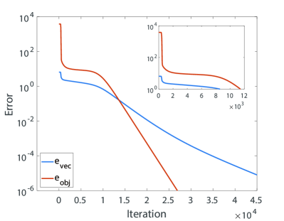
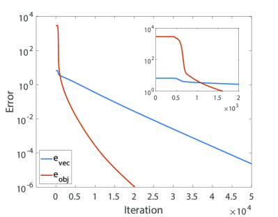
Figure 1: Convergence behavior of two tests, each are depicted with $e_{\text{vec}}$ and $e_{\text{obj}}$. The first few iterations are zoomed in on their top right corners.

Since the initial points are chosen near some saddle points, in the first few iterations, the error decays slowly, and the linear convergence rate is not guaranteed. After $X^{(t)}$ escapes from the saddle point near the initial point, it may fall into the domain of local linear convergence directly (Figure 1 right) or slow down several times before linear convergence (Figure 1 left), which depends on the choice of initial points. According to our analysis, the slow-down happens a finite number of times, and the iteration will converge monotonically to the global minima. All of our experiments, including the two in Figure 1 agree well with our analysis.

Acknowledgments. The authors thank Jianfeng Lu and Zhe Wang for helpful discussions. YL is supported in part by the US Department of Energy via grant de-sc0019449. WG is supported in part by National Science Foundation of China under Grant No. 11690013, U1811461.

Appendix A Proof of Lemma 3.1

Proof A.1.

It is sufficient to show that the condition holds for one iteration. In order to simplify the notations, we denote $x_{i}^{(t)}$ and $x_{i}^{(t+1)}$ as $x_{i}$ and $\widetilde{x}_{i}$ respectively. The norms of $x_{i}$ and $\widetilde{x}_{i}$ are denoted as $r_{i}$ and $\widetilde{r}_{i}$ respectively.

The iteration in (7) can be written as,

$$\widetilde{x}_{i}=x_{i}-\alpha Ax_{i}-\alpha(\sum_{j=1}^{i}x_{j}x_{j}^{\top})x_{i}=x_{i}-\alpha\widetilde{A}x_{i}-\alpha x_{i}x_{i}^{\top}x_{i}.$$ (64)

where $\widetilde{A}=A+\sum_{j=1}^{i-1}x_{j}x_{j}^{\top}$. The norm square of $\widetilde{x}_{i}$ can be calculated as,

$$\widetilde{r}_{i}^{2}=\widetilde{x}_{i}^{\top}\widetilde{x}_{i} =x_{i}^{\top}x_{i}-2\alpha\left(x_{i}^{\top}\widetilde{A}x_{i}+(x_{i}^{\top}x_{i})^{2}\right)$$

$$\quad+\alpha^{2}\left(x_{i}^{\top}\widetilde{A}^{\top}\widetilde{A}x_{i}+(x_{i}^{\top}x_{i})^{3}+2x_{i}^{\top}\widetilde{A}x_{i}(x_{i}^{\top}x_{i})\right)$$

$$=r_{i}^{2}-2\alpha\left(x_{i}^{\top}\widetilde{A}x_{i}+r_{i}^{4}\right)+\alpha^{2}\left(x_{i}^{\top}\widetilde{A}^{\top}\widetilde{A}x_{i}+r_{i}^{6}+2x_{i}^{\top}\widetilde{A}x_{i}r_{i}^{2}\right).$$ (65)

Given that all $x_{i}$ satisfy the conditions $\left\|x_{i}\right\|\leq R_{i}$, we have inequality for any vector $x$ and power $k$,

$$-\left(\rho+\sum_{j=1}^{i-1}R_{j}^{2}\right)^{k}\left\|x\right\|^{2}\leq x^{\top}\widetilde{A}^{k}x\leq\left(\rho+\sum_{j=1}^{i-1}R_{j}^{2}\right)^{k}\left\|x\right\|^{2},$$ (66)

where we adopt the definition of eigenvalues for the first part in $\widetilde{A}$ and Cauchy-Schwartz inequality for the second part in $\widetilde{A}$. Due to the assumption on $R_{j}$, we can bound the growing factor in (66) as,

$$\rho+\sum_{j=1}^{i-1}R_{j}^{2}\leq\rho\left(1+3\sum_{j=1}^{i-1}4^{j-1}\right)\leq 4^{i-1}\rho=\frac{R_{i}^{2}}{3}.$$ (67)

With these inequalities, the first order term of $\alpha$ in (A.1) can be bounded as,

$$-2\alpha\left(x_{i}^{\top}\widetilde{A}x_{i}+r_{i}^{4}\right)\leq 2\alpha r_{i}^{2}\left(\frac{R_{i}^{2}}{3}-r_{i}^{2}\right).$$ (68)

And the second order term can be bounded as,

$$\alpha^{2}\left(x_{i}^{\top}\widetilde{A}^{2}x_{i}+r_{i}^{6}+2x_{i}^{\top}\widetilde{A}x_{i}r_{i}^{2}\right) \leq\alpha^{2}\left(\left(\rho+\sum_{j=1}^{i-1}R_{j}^{2}\right)^{2}r_{i}^{2}+r_{i}^{6}+2\left(\rho+\sum_{j=1}^{i-1}R_{j}^{2}\right)r_{i}^{4}\right)$$

$$\leq\alpha^{2}r_{i}^{2}\left(\frac{R_{i}^{4}}{9}+r_{i}^{4}+\frac{2R_{i}^{2}}{3}r_{i}^{2}\right).$$ (69)

The rest of the proof is divided into two scenarios, i.e., $r_{i}\in[\frac{\sqrt{2}R_{i}}{\sqrt{3}},R_{i}]$ and $r_{i}\in[0,\frac{\sqrt{2}R_{i}}{\sqrt{3}})$.

In the first scenario, $r_{i}\in[\frac{\sqrt{2}R_{i}}{\sqrt{3}},R_{i}]$, we have $-2\alpha\left(x_{i}^{\top}\widetilde{A}x_{i}+r_{i}^{4}\right)\leq-\alpha r_{i}^{2}\frac{2R_{i}^{2}}{3}$ for the first order term. Applying $\alpha\leq\frac{1}{5R_{p}^{2}}$, we have,

$$\widetilde{r}_{i}^{2}\leq r_{i}^{2}+\alpha r_{i}^{2}\left(-\frac{2R_{i}^{2}}{3}+\frac{R_{i}^{4}}{45R_{p}^{2}}+\frac{R_{i}^{4}}{5R_{p}^{2}}+\frac{2R_{i}^{4}}{15R_{p}^{2}}\right)\leq r_{i}^{2}-\alpha r_{i}^{2}\frac{14R_{i}^{2}}{45}<r_{i}^{2}\leq R_{i}^{2}.$$ (70)

In the second scenario, $r_{i}\leq\sqrt{\frac{2}{3}}R_{i}$, we have

$$\widetilde{r}_{i}^{2} \leq r_{i}^{2}+2\alpha r_{i}^{2}\left(\frac{R_{i}^{2}}{3}-r_{i}^{2}\right)+\alpha^{2}r_{i}^{2}\left(\frac{R_{i}^{4}}{9}+r_{i}^{4}+\frac{2R_{i}^{2}}{3}r_{i}^{2}\right)$$

$$\leq\frac{2R_{i}^{2}}{3}+\frac{4R_{i}^{4}}{45R_{p}^{2}}+\frac{2R_{i}^{6}}{675R_{p}^{4}}+\frac{8R_{i}^{6}}{675R_{p}^{4}}+\frac{8R_{i}^{6}}{675R_{p}^{4}}<R_{i}^{2}.$$ (71)

This proves the lemma.

Appendix B Proof of Lemma 4.12

Proof B.1.

Without loss of generality, we assume $A$ is diagonal. Notations remain the same as that in the proof of Lemma 4.6 if not redefined. Based on the assumptions, we denote $k\in(i,q]$ as the smallest integer such that $e_{k}^{\top}x_{i}^{(t)}=x_{ik}^{(t)}$ does not converge to zero. Hence, there exists a positive number $\delta>0$ such that for any $N$, there exists a $t>N$ and $\absolutevalue{x_{ik}^{(t)}}>\delta$. We also know that Lemma 4.8 holds, $\left\|E^{(t)}\right\|$ converges to zero, and $e_{j}^{\top}x_{i}^{(t)}=x_{ij}^{(t)}$ converges to zero for all $j\in[1,i)\cup(p,n]$. Hence, for any $\varepsilon$ sufficiently small, there exists an integer $N_{1}$ such that $\left\|E^{(t)}\right\|\leq\varepsilon^{2}$, $\left\|x_{i}^{(t)}\right\|\geq\frac{\sqrt{-2\lambda_{q}}}{4}$, and $\absolutevalue{x_{ij}^{(t)}}\leq\varepsilon$ hold for all $t>N_{1}$ and $j\in[1,i)\cup(p,n]$. Since $e_{j}^{\top}x_{i}^{(t)}=x_{ij}^{(t)}$ does not converge to zero, there exists an integer $N_{2}>N_{1}$, such that,

$$\frac{\absolutevalue{x_{ij}^{(N_{2})}}}{\left\|x_{i}^{(N_{2})}\right\|}\geq\frac{\delta}{R_{i}}\geq\frac{2\varepsilon^{2}}{\lambda_{j+1}-\lambda_{j}}.$$ (72)

Using the iterative relationship (27), we have the lower bound on $\absolutevalue{x_{ij}^{(N_{2}+1)}}$,

$$\absolutevalue{x_{ij}^{(N_{2}+1)}}\geq\left(1-\alpha\frac{\lambda_{j}+\lambda_{j+1}}{2}-\alpha\left\|x_{i}^{(N_{2})}\right\|^{2}\right)\absolutevalue{x_{ij}^{(N_{2})}}.$$ (73)

Again using the iterative relationship (27), we provide the upper bound for

$$\sqrt{\sum_{j\neq k}\left(x_{ij}^{(N_{2}+1)}\right)^{2}} \leq\Bigg{\{}\sum_{j<i}\left(1-\alpha\left\|x_{i}^{(N_{2})}\right\|^{2}\right)^{2}\left(x_{ij}^{(N_{2})}\right)^{2}$$

$$\quad+\sum_{i\leq j<k}\left(1-\alpha\lambda_{j}-\alpha\left\|x_{i}^{(N_{2})}\right\|^{2}\right)^{2}\varepsilon^{2}$$

$$\quad+\sum_{j>k}\left(1-\alpha\lambda_{k+1}-\alpha\left\|x_{i}^{(N_{2})}\right\|^{2}\right)^{2}\left(x_{ij}^{(N_{2})}\right)^{2}\Bigg{\}}^{\frac{1}{2}}+3\sqrt{\alpha n}R_{i}\varepsilon$$

$$\leq\left(1-\alpha\lambda_{k+1}-\alpha\left\|x_{i}^{(N_{2})}\right\|^{2}\right)\sqrt{\sum_{j\neq k}\left(x_{ij}^{(N_{2})}\right)^{2}}+\sqrt{n}\varepsilon+3\sqrt{\alpha n}R_{i}\varepsilon,$$ (74)

where the derivation is slightly different from that in (4.11), The first inequality adopts similar derivation in (4.11) while keeps the first term unchanged; and the second inequality mainly uses the inequality of square-root function.

Substituting (73) and (B.1) into the expression of $\tan\theta_{k}^{(N_{2}+1)}$, we obtain,

$$\tan\theta_{k}^{(N_{2}+1)}\leq(1-\beta)\tan\theta_{k}^{(N_{2})}-\beta\tan\theta_{k}^{(N_{2})}+C\varepsilon,$$ (75)

where $\beta=\frac{\alpha(\lambda_{i+1}-\lambda_{i})}{4-2\alpha(\lambda_{i}+\lambda_{i+1})}\in(0,1)$ and $C=\frac{8\sqrt{n}R_{i}+24\sqrt{\alpha n}R_{i}^{2}}{\sqrt{-2\lambda_{q}}\delta}$.

Based on the last inequality in (75), if $\tan\theta_{k}^{(N_{2})}>\frac{C\varepsilon}{\beta}$, than we have $\tan\theta_{k}^{(N_{2}+1)}<(1-\beta)\tan\theta_{k}^{(N_{2})}$, which implies $\cos\theta_{k}^{(N_{2}+1)}>\cos\theta_{k}^{(N_{2})}$ due to the fact that all angles acute angle. Therefore, (72) holds for $t=N_{2}+1$ and $\tan\theta_{k}^{(t)}$ decay monotonically until $\tan\theta_{k}^{(t)}\leq\frac{C\varepsilon}{\beta}$. When $\tan\theta_{k}^{(t)}\leq\frac{C\varepsilon}{\beta}$, we obviously have $\tan\theta_{k}^{(t+1)}\leq\frac{C\varepsilon}{\beta}$. The inequality condition (4.11) still holds as long as $\varepsilon$ is sufficiently small. Hence there exists a $N$ such that for all $t>N$, we have $\tan\theta_{k}^{(t+1)}\leq\frac{C\varepsilon}{\beta}$, which can be arbitrarily small.

Appendix C Proof of Lemma 4.20

Proof C.1.

This lemma is proved in a similar way as that of Lemma 4.18. If the lemma does not hold, there is some $t^{\prime}\in(t_{1},t_{2})$ such that $\left\|x_{i}^{\left(t^{\prime}\right)}-s\right\|\geq 6\sqrt{n}\varepsilon_{i}^{\frac{1}{3}}$. Let $t_{1}^{\prime}\in(t_{1},t^{\prime}]$ be the latest time such that $x_{i}^{\left(t_{1}^{\prime}-1\right)}\in\mathcal{N}$ and $x_{i}^{\left(t_{1}^{\prime}\right)}\not\in\mathcal{N}$ for $\mathcal{N}=\mathcal{N}_{s,\varepsilon_{i}}$. Also let $t_{2}^{\prime}\in(t^{\prime},t_{2}]$ be the first time such that $x_{i}^{\left(t_{2}^{\prime}\right)}\in\mathcal{N}$. Then we have,

$$\left\|\nabla{F\left(x_{i}^{\left(t_{1}^{\prime}-1\right)}\right)}\right\|<\varepsilon_{i},\quad\left\|x_{i}^{\left(t_{1}^{\prime}-1\right)}-s\right\|<\sqrt{n}\varepsilon_{i}^{\frac{1}{3}},\quad\left\|\nabla{F\left(x_{i}^{\left(t_{1}^{\prime}\right)}\right)}\right\|\geq\varepsilon_{i},$$

$$\left\|\nabla{F\left(x_{i}^{\left(t_{2}^{\prime}\right)}\right)}\right\|<\varepsilon_{i},\quad\left\|x_{i}^{\left(t_{2}^{\prime}\right)}-s\right\|<\sqrt{n}\varepsilon_{i}^{\frac{1}{3}}.$$ (76)

By the construction of $t^{\prime}_{1}$ and $t_{2}^{\prime}$, we know that for all $t\in[t^{\prime}_{1},t_{2}^{\prime})$, $x_{i}^{(t)}\not\in\mathcal{N}$. Adopting the same derivation as in (60), we obtain a lower bound on the function difference,

$$F\left(x_{i}^{\left(t_{1}^{\prime}\right)}\right)-F\left(x_{i}^{\left(t_{2}^{\prime}\right)}\right)\leq 3\sqrt{n}\varepsilon_{i}^{\frac{4}{3}}.$$ (77)

On the other hand, lower bound of the energy function decrement for $x_{i}^{\left(t_{1}^{\prime}\right)},\dots,x_{i}^{\left(t_{2}^{\prime}\right)}$ can be estimated as, according to Lemma 4.14,

$$F\bigg{(}x_{i}^{\left(t_{1}^{\prime}\right)}\bigg{)}-F\bigg{(}x_{i}^{\left(t_{2}^{\prime}\right)}\bigg{)} >\frac{1}{2}\varepsilon_{i}\left(\sum_{t=t_{1}^{\prime}}^{t^{\prime}-1}\left(\left\|x_{i}^{(t)}-x_{i}^{(t+1)}\right\|\right)+\sum_{t=t^{\prime}}^{t_{2}^{\prime}}\left(\left\|x_{i}^{(t)}-x_{i}^{(t+1)}\right\|\right)\right)$$

$$\geq\frac{1}{2}\varepsilon_{i}\Bigg{(}\left\|x_{i}^{\left(t_{1}^{\prime}-1\right)}-x_{i}^{\left(t^{\prime}\right)}\right\|+\left\|x_{i}^{\left(t_{2}^{\prime}\right)}-x_{i}^{\left(t^{\prime}\right)}\right\|-\left\|x_{i}^{\left(t_{1}^{\prime}-1\right)}-x_{i}^{\left(t_{1}^{\prime}\right)}\right\|\Bigg{)}$$

$$>4\sqrt{n}\varepsilon_{i}^{\frac{4}{3}},$$ (78)

where the last inequality is based on (C.1) and $\left\|x_{i}^{\left(t^{\prime}\right)}-s\right\|\geq 6\sqrt{n}\varepsilon_{i}^{\frac{1}{3}}$. Thus the contradiction is derived.

References

- Chen et al., [2021] Chen, Z., Li, Y., and Lu, J. (2021). On the global convergence of randomized coordinate gradient descent for non-convex optimization. https://arxiv.org/abs/2101.01323v1.
- Corsetti, [2014] Corsetti, F. (2014). The orbital minimization method for electronic structure calculations with finite-range atomic basis sets. Comput. Phys. Commun., 185(3):873–883.
- Fattahi et al., [2020] Fattahi, S., Sojoudi, S., and Schmidt, M. (2020). Exact guarantees on the absence of spurious local minima for non-negative rank-1 robust principal component analysis. J. Mach. Learn. Res., 21:1–51.
- Froyland et al., [2015] Froyland, G., González-Tokman, C., and Quas, A. (2015). Stochastic stability of Lyapunov exponents and Oseledets splittings for semi-invertible matrix cocycles. Commun. Pure Appl. Math., 68(11):2052–2081.
- Gang and Bajwa, [2022] Gang, A. and Bajwa, W. U. (2022). A linearly convergent algorithm for distributed principal component analysis. Signal Processing, 193:108408.
- Gang et al., [2019] Gang, A., Raja, H., and Bajwa, W. U. (2019). Fast and communication-efficient distributed pca. In ICASSP 2019-2019 IEEE International Conference on Acoustics, Speech and Signal Processing (ICASSP), pages 7450–7454. IEEE.
- Gao et al., [2021] Gao, W., Li, Y., and Lu, B. (2021). Triangularized orthogonalization-free method for solving extreme eigenvalue problems. https://arxiv.org/abs/2005.12161.
- Ge et al., [2017] Ge, R., Jin, C., and Zheng, Y. (2017). No spurious local minima in nonconvex low rank problems: A unified geometric analysis. In Precup, D. and Teh, Y. W., editors, Proc. 34th Int. Conf. Mach. Learn., volume 70 of Proceedings of Machine Learning Research, pages 1233–1242. PMLR.
- Ge et al., [2016] Ge, R., Lee, J. D., and Ma, T. (2016). Matrix completion has no spurious local minimum. In Adv. Neural Inf. Process. Syst., volume 29.
- Hardt and Price, [2014] Hardt, M. and Price, E. (2014). The noisy power method: A meta algorithm with applications. In Ghahramani, Z., Welling, M., Cortes, C., Lawrence, N., and Weinberger, K. Q., editors, Advances in Neural Information Processing Systems, volume 27. Curran Associates, Inc.
- Laio and Parrinello, [2002] Laio, A. and Parrinello, M. (2002). Escaping free–energy minima. Proc. Natl. Acad. Sci., 99(20):12562–6.
- Ledrappier and Young, [1991] Ledrappier, F. and Young, L. S. (1991). Stability of Lyapunov exponents. Ergod. Theory Dyn. Syst., 11(3):469–484.
- Lee et al., [2019] Lee, J. D., Panageas, I., Piliouras, G., Simchowitz, M., Jordan, M. I., and Recht, B. (2019). First-order methods almost always avoid strict saddle points. Math. Program., 176(1-2):311–337.
- Li et al., [2019] Li, Y., Lu, J., and Wang, Z. (2019). Coordinatewise descent methods for leading eigenvalue problem. SIAM J. Sci. Comput., 41(4):A2681–A2716.
- Lu and Thicke, [2017] Lu, J. and Thicke, K. (2017). Orbital minimization method with l1 regularization. J. Comput. Phys., 336:87–103.
- Lu and Yang, [2017] Lu, J. and Yang, H. (2017). Preconditioning orbital minimization method for planewave discretization. Multiscale Model. Simul., 15(1):254–273.
- Wen et al., [2016] Wen, Z., Yang, C., Liu, X., and Zhang, Y. (2016). Trace-penalty minimization for large-scale eigenspace computation. J. Sci. Comput., 66(3):1175–1203.