Nonnegative spatial factorization

Abstract

Gaussian processes are widely used for the analysis of spatial data due to their nonparametric flexibility and ability to quantify uncertainty, and recently developed scalable approximations have facilitated application to massive datasets. For multivariate outcomes, linear models of coregionalization combine dimension reduction with spatial correlation. However, their real-valued latent factors and loadings are difficult to interpret because, unlike nonnegative models, they do not recover a parts-based representation. We present nonnegative spatial factorization (NSF), a spatially-aware probabilistic dimension reduction model that naturally encourages sparsity. We compare NSF to real-valued spatial factorizations such as MEFISTO (Velten et al., 2020) and nonspatial dimension reduction methods using simulations and high-dimensional spatial transcriptomics data. NSF identifies generalizable spatial patterns of gene expression. Since not all patterns of gene expression are spatial, we also propose a hybrid extension of NSF that combines spatial and nonspatial components, enabling quantification of spatial importance for both observations and features. A TensorFlow implementation of NSF is available from https://github.com/willtownes/nsf-paper.

Keywords: spatial, multivariate, dimension reduction, nonnegative, Gaussian process, spatial transcriptomics

1 Introduction

Spatially-resolved transcriptomics (ST) has revolutionized the study of intact biological tissues (Moses and Pachter, 2021; Editors, 2021; Maynard et al., 2021). In contrast to single-cell RNA sequencing (scRNA-seq), which dissociates cells before sequencing each one, ST quantifies gene expression while preserving the spatial context of the cells within the tissue sample. Since the state and function of each cell is highly dependent upon interactions with its neighbors (Verma et al., 2021), measuring spatially-resolved transcription represents a crucial advance in our ability to understand cellular state and interactions.

Like scRNA-seq, ST data generally consist of discrete counts of transcripts from tens to thousands of genes, many of which are zero. Also, in both techniques there is typically no ground truth assignment of cell types. There are two basic strategies to measure spatial gene expression: microscopy and bead capture. Microscopy approaches have excellent spatial resolution, even at the sub-cellular level, but require specialized equipment and may not capture large numbers of cells or genes easily. Examples of microscopy protocols include seqFISH+ (Eng et al., 2019) and MERFISH (Xia et al., 2019). Protocols based on bead capture and sequencing tend to have coarser spatial resolution but cover larger spatial areas or larger numbers of genes. They are popular because they use equipment and experimental procedures that are similar to single-cell RNA-seq (scRNA-seq). Examples of bead protocols include high definition spatial transcriptomics (HDST) (Vickovic et al., 2019), Slide-seqV2 (Stickels et al., 2021), and the Visium platform from 10x genomics.

Dimension reduction (DR) is a vital tool for unsupervised learning, and there has been a proliferation of DR methods for both scRNA-seq (Wolf et al., 2017; Butler et al., 2018; Sun et al., 2019) and ST (Palla et al., 2021; Dries et al., 2021). DR based on a Gaussian error assumption, such as principal components analysis (PCA) (Hotelling, 1933) and factor analysis (Bartholomew et al., 2011), is often computationally fast, but requires elaborate normalization procedures that may systematically distort the count data from sequencing technologies (Hicks et al., 2018; Townes et al., 2019a). For example, this has led to confusion about whether zero-inflated distributions are needed to analyze scRNA-seq data, or whether the high number of zeros is consistent with a simpler Poisson or negative binomial count distribution (Svensson, 2020; Kim et al., 2020; Sarkar and Stephens, 2020). To avoid normalization and its pitfalls, DR approaches such as scVI (Lopez et al., 2018), CPLVM (Jones et al., 2021), and GLM-PCA (Townes et al., 2019b) operate directly on raw counts of unique molecular identifiers (UMIs) by assuming appropriate likelihoods such as the Poisson or negative binomial.

Since ST data, like scRNA-seq, are high-dimensional molecule counts that map onto specific gene transcripts, in principle existing DR methods can be used to obtain a low-dimensional representation of gene expression at each spatial location. This is in fact the standard procedure recommended by tutorials from two popular packages: Seurat and Scanpy. However, this application of scRNA-seq methods ignores the spatial coordinates that are the distinguishing feature of ST. We would instead like to retain spatial locality information while performing DR on these data.

Gaussian processes (GPs) are probability distributions over arbitrary functions on a continuous (e.g., spatial) domain (Rasmussen and Williams, 2005). GPs are a fundamental tool in spatial statistics (Banerjee et al., 2014; Cressie and Moores, 2021). Historically, GPs have been widely used in environmental applications with spatial structure (Finley et al., 2019). In the genomics (ST) context, spatialDE (Svensson et al., 2018) fits univariate GP models to ST data to identify which genes are spatially variable. Other examples of univariate GPs applied to ST data include the Bayesian hierarchical model Splotch (Äijö et al., 2019) and the scalable GPcounts (BinTayyash et al., 2021). While these methods make positive steps toward including spatial information in routine ST analyses, they do not provide dimension reduction. Genes do not act in isolation but interact with each other. This means there is substantial gene-gene correlation in multivariate ST data ignored by univariate approaches.

A multivariate approach to spatially-aware dimension reduction for ST data is provided by MEFISTO (Velten et al., 2020). The key concept of MEFISTO is to represent the high-dimensional gene expression features as a linear combination of a small number of independent GPs over the spatial domain. This is known in the statistics literature as a linear model of coregionalization (LMC) (Gelfand et al., 2004). Historically, LMC factorization required a conjugate (Gaussian) likelihood for computational tractability, which is not appropriate for ST count data. Following Yu et al. (2009), we refer to this model as Gaussian process factor analysis (GPFA). In neuroscience, attempts were made to relax the Gaussian assumption for application to functional MRI data, leading to count-GPFA Zhao and Park (2017).

Even with conjugate likelihoods and univariate outcomes, exact inference for GPs scales cubically with the number of observations (or spatial locations), which is often prohibitive for ST. For example, the recent Slide-seqV2 protocol can generate tens of thousands of observations (Stickels et al., 2021). Breakthroughs in variational inference for GPs have greatly improved scalability and enabled nonconjugate likelihoods through approximate inference with inducing points (IPs; see Leibfried et al. (2021) and van der Wilk et al. (2020) for overviews). GPFlow is a popular implementation supporting a variety of likelihoods (Matthews et al., 2017). MEFISTO also uses the variational IP strategy, and in principle is compatible with nonconjugate likelihoods, but in practice the authors recommend using a Gaussian likelihood (Velten et al., 2020). An alternative to IPs using polynomial approximate likelihoods (Huggins et al., 2017) has been proposed for count-GPFA (Keeley et al., 2020).

The latent, low-dimensional spatial factors discovered by LMC variants such as GPFA, count-GPFA, and MEFISTO are real-valued. Thus, they may be thought of as spatial analogs of PCA (when the data likelihood is Gaussian) and GLM-PCA (for non-Gaussian data likelihoods). In all cases, latent factors are combined linearly to predict the outcomes. We refer to the weights in these linear combinations as loadings, and note that, in the models described above, these loadings are assumed to be real-valued as well. We will use the terms real-valued spatial factorization (RSF) and factor analysis (FA) to refer to these spatial and nonspatial models, respectively. Both RSF and FA models tend to produce dense loadings, but MEFISTO counteracts this with sparsity-promoting priors on the loadings matrix. Sparse loadings are more interpretable than dense because, through nonzero values in the loadings, they assign a small number of relevant features to each component, rather than matching every feature to every component.

Another way to generate sparse loadings is to constrain the entire model to be nonnegative. In the non-spatial context, nonnegative matrix factorization (NMF) (Lee and Seung, 1999) and latent Dirichlet allocation (LDA) (Blei et al., 2003) are widely used to produce interpretable low-dimensional factorizations of high-dimensional count data (Carbonetto et al., 2021) including scRNA-seq (Elyanow et al., 2020; Sherman et al., 2020) and ST (Zeira et al., 2021). To quantify uncertainty, a Bayesian prior can be placed on latent factors and a Poisson or negative binomial data likelihood included to lead to probabilistic NMF (PNMF). The advantage of PNMF over real-valued alternatives is that, for geometric reasons, they produce parts-based representations rather than holistic representations. For example, when decomposing pixel-based representations of faces, PNMF decomposes a face into factors representing eyes, noses, mouths, and ears distinctly (Lee and Seung, 1999). On the other hand, real-valued alternatives produce eigenfaces, or representations of whole faces in each factor (Lee and Seung, 1999). Incorporating nonnegativity constraints into spatial models is not straightforward, though, since GPs are inherently real-valued.

The contributions of this work are threefold. First, we develop nonnegative spatial factorization (NSF), a model that allows spatially-aware dimension reduction using a Gaussian process prior over the spatial locations and with a Poisson or negative binomial likelihood for count data. Second, we combine this spatially-aware dimension reduction with nonspatial factors in a NSF hybrid model (NSFH) to partition variability into the spatial and nonspatial sources. Finally, we identify appropriate GP kernels and develop inference methods for the kernel parameters and latent variables to enable computationally tractable fitting of large field-of-view ST data.

This paper proceeds as follows. We first define the generative models of FA, PNMF, RSF, NSF, and NSFH. Secondly, we illustrate the ability of nonnegative factorizations to identify a parts-based representation using simulations. We then describe the basic features of the ST datasets and examine key results of a benchmarking comparison of different models. Next, we analyze three ST datasets from different technologies with NSFH and show how to interpret the spatial and nonspatial components. We conclude with a discussion of the implications of our results in ST data analysis and promising directions for future studies. Details on inference and parameter estimation, procedures for postprocessing nonnegative factor models and computing spatial importance scores, and data preprocessing are provided in the Methods section.

2 Results

2.1 Factor models for spatial count data

Table 1: Summary of probabilistic factor models for high-dimensional spatial count data. An X in the nonnegative, spatial, or nonspatial column indicates whether the model includes that type of latent factors. Likelihoods are listed with the default choice of each model first. gau: Gaussian or normal distribution, poi: Poisson, nb: negative binomial.

abbrev	model	nonnegative	spatial	nonspatial	likelihoods
FA	factor analysis			X	gau
PNMF	probabilistic nonnegative matrix factorization	X		X	poi, nb, gau
MEFISTO	MEFISTO		X		gau, poi
RSF	real-valued spatial factorization		X		gau
NSF	nonnegative spatial factorization	X	X		poi, nb, gau
NSFH	nonnegative spatial factorization hybrid	X	X	X	poi, nb, gau

The data consist of a multivariate outcome $Y\in\mathbb{R}^{N\times J}$ and spatial coordinates $X\in\mathbb{R}^{N\times D}$. Let $i=1,\ldots,N$ index the observations (e.g., cells, spots, or locations with a single $(x,y)$ coordinate value), $j=1,\ldots,J$ index the outcome features (e.g., genes), and $d=1\ldots,D$ index the spatial input dimensions.

2.1.1 Nonspatial models

In unsupervised dimension reduction such as PCA or NMF, the goal is to represent $Y$ (or a normalized version $\tilde{Y}$) as the product of two low-rank matrices $Y\approx FW^{\prime}$, where the factors matrix $F$ has dimension $N\times L$ and the loadings matrix $W$ has dimension $J\times L$, with $L\ll J$. Let $l=1,\ldots,L$ index over the components. A probabilistic version of PCA is factor analysis (FA):

$$\tilde{y}_{ij} \sim\mathcal{N}(\mu_{ij},~{}\sigma_{j}^{2})$$

$$\mu_{ij} =\sum_{l=1}^{L}w_{jl}f_{il}$$

$$f_{il} \sim\mathcal{N}(m_{l},~{}s^{2}_{l}).$$

A probabilistic version of NMF is probabilistic nonnegative matrix factorization (PNMF):

$$y_{ij} \sim Poi(\nu_{i}\lambda_{ij})$$

$$\lambda_{ij} =\sum_{l=1}^{L}w_{jl}e^{f_{il}}$$

$$f_{il} \sim\mathcal{N}(m_{l},~{}s^{2}_{l}),$$

where $\nu_{i}$ indicates a fixed size factor to account for differences in total counts per observation. In both of these unsupervised models, the prior on the factors $f_{il}$ assumes each observation is an independent draw and ignores spatial information $\bm{x}_{i}$.

2.1.2 Spatial process factorization

In spatial process factorization, we assume that spatially adjacent observations should have correlated outcomes. We encode this assumption via a Gaussian process (GP) prior over the factors. We define real-valued spatial factorization (RSF) as

$$\tilde{y}_{ij} \sim\mathcal{N}(\mu_{ij},~{}\sigma_{j}^{2})$$

$$\mu_{ij} =\sum_{l=1}^{L}w_{jl}f_{il}$$

$$f_{il} =f_{l}(\bm{x}_{i})\sim GP\big{(}\mu_{l}(\bm{x}_{i}),~{}k_{l}(\bm{x}_{i},X)\big{)},$$

where $\mu_{l}(\cdot)$ indicates a parametric mean function and $k_{l}(\cdot,\cdot)$ a positive semidefinite covariance (kernel) function. In our implementation, we specify the mean function as a linear function of the spatial coordinates,

$$\mu_{l}(\bm{x}_{i})=\beta_{0l}+\bm{x}_{i}^{\prime}\bm{\beta}_{1l}.$$

For the covariance function, we choose a Matérn kernel with fixed smoothness parameter $3/2$. We allow each component $l$ to have its own amplitude and length-scale parameters that we estimate from data. RSF is a spatial analog to factor analysis. MEFISTO has the same structure as RSF, but uses a squared exponential kernel instead of Matérn, and further places a sparsity-promoting prior on the loading weights $w_{jl}$. Our implementation is modular and can accept any positive semidefinite kernel. However, we found the Matérn kernel to have better numerical stability than the squared exponential in our experiments.

Nonnegative spatial factorization (NSF) is a spatial analog of probabilistic NMF (PNMF).

$$y_{ij} \sim Poi(\nu_{i}\lambda_{ij})$$

$$\lambda_{ij} =\sum_{l=1}^{L}w_{jl}e^{f_{il}}$$

$$f_{il} =f_{l}(\bm{x}_{i})\sim GP\big{(}\mu_{l}(\bm{x}_{i}),~{}k_{l}(\bm{x}_{i},X)\big{)}.$$

For NSF, we use the same mean and kernel functions as RSF, but we additionally constrain the weights $w_{jl}\geq 0$.

We sought to quantify the relative importance of spatial versus nonspatial variation by combining NSF and PNMF into a semisupervised framework we refer to as the nonnegative spatial factorization hybrid model (NSFH). NSFH consists of $L$ total factors, $T\leq L$ of which are spatial and $L-T$ are nonspatial. We recover NSF and PNMF as special cases when $T=L$ or $T=0$, respectively. By default, we set $T=L/2$.

$$y_{ij} \sim Poi(\nu_{i}\lambda_{ij})$$

$$\lambda_{ij} =\sum_{l=1}^{T}w_{jl}e^{f_{il}}+\sum_{l=T+1}^{L}v_{jl}e^{h_{il}}$$

$$f_{il} =f_{l}(\bm{x}_{i})\sim GP\big{(}\mu_{l}(\bm{x}_{i}),~{}k_{l}(\bm{x}_{i},X)\big{)}$$

$$h_{il} \sim\mathcal{N}(m_{l},~{}s^{2}_{l}).$$

Our implementations of PNMF, NSF, and NSFH are modular with respect to the likelihood, so that the negative binomial or Gaussian distributions can be substituted for the Poisson. However, in our experiments we use the Poisson data likelihood.

2.1.3 Postprocessing nonnegative factor models

We postprocess fitted nonnegative models (PNMF, NSF, and NSFH) by projecting factors and loadings onto a simplex. This highlights features (genes) that are enriched in particular components rather than those with high expression across all components. In the NSFH model, we interpret the ratio of loadings weights for each feature across all spatial components as a spatial importance score. This is analogous to the proportion of variance explained in PCA. In particular, a score of $1$ means that variation in a gene’s expression profile across all observations is completely captured by the spatial factors, whereas a $0$ means that expression variation is completely captured by nonspatial factors. The gene-level scores can be used to identify spatially variable genes as pioneered by spatialDE (Svensson et al., 2018). We also compute observation-level scores by switching the role of the factors and loadings matrices; details are provided in the Methods.

2.2 Simulations: Nonnegative factorizations identify parts-based representation

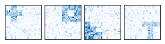
(b) simulated count data

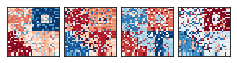
(c) factor analysis

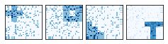
(d) probabilistic nonnegative matrix factorization

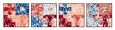
(e) MEFISTO

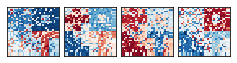
(f) real-valued spatial factorization

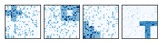
(g) nonnegative spatial factorization

(h) nonnegative spatial factorization hybrid model

Figure S1: Nonnegative factorizations recover a parts-based representation in “ggblocks” simulated multivariate spatial count data. (a) Each of $500$ features was randomly assigned to one of four nonnegative spatial factors. (b) Negative binomial count data used for model fitting. (c) Real-valued factors learned from unsupervised (nonspatial) dimension reduction. (d) as (c) but using nonnegative components. (e) Real-valued, spatially-aware factors with squared exponential kernel. (f) as (e) but with Matérn kernel. (g) Nonnegative, spatially-aware factors. (h) as (g) but with additional three nonspatial factors.

To illustrate the ability of nonnegative models to recover a parts-based factorization, we simulated multivariate count data from two sets of spatial patterns. The “ggblocks” simulation was based on the Indian buffet process (IBP) Griffiths and Ghahramani (2011). The true factors consisted of four simple shapes in different spatial regions. In the “quilt” simulation, we created spatial patterns that overlapped in space. For both simulations, each of the $500$ features was an independent negative binomial draw from one of the canonical patterns (Figures S1a,b and 1a,b). Real-valued models FA, MEFISTO, and RSF estimated latent factors consisting of linear combinations of the true factors (Figures S1c,e,f and 1c,e,f). Nonnegative models PNMF, NSF, and NSFH identified each pattern as a separate factor (Figures S1d,g,h and 1d,g,h). This suggests that the parts-based representation in PNMF is preserved in NSF and NSFH.

(a) ground truth

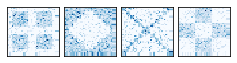
(b) simulated count data

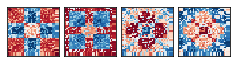
(c) factor analysis

(d) probabilistic nonnegative matrix factorization

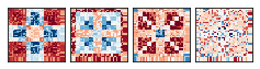
(e) MEFISTO

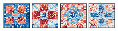
(f) real-valued spatial factorization

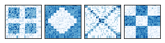
(g) nonnegative spatial factorization

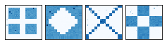
(h) nonnegative spatial factorization hybrid model

Figure 1: Nonnegative factorizations recover a parts-based representation in “quilt” simulated multivariate spatial count data. (a) Each of $500$ features was randomly assigned to one of four nonnegative spatial factors. (b) Negative binomial count data used for model fitting. (c) Real-valued factors learned from unsupervised (nonspatial) dimension reduction. (d) as (c) but using nonnegative components. (e) Real-valued, spatially-aware factors with squared exponential kernel. (f) as (e) but with Matérn kernel. (g) Nonnegative, spatially-aware factors. (h) as (g) but with additional three nonspatial factors.

2.3 Application to spatial transcriptomics datasets

We examined the goodness-of-fit and interpretability of nonnegative spatial factorizations on three spatial transcriptomics datasets (Table 2). The Slide-seqV2 hippocampus data (Stickels et al., 2021) consists of $36,536$ observations, each at a unique location. The XYZeq liver data (Lee et al., 2021b) consists of $2,700$ observations at $289$ unique locations. Unlike the other protocols, each observation represents a single cell, but multiple cells are assigned to the same location. In other words, each spatial location in XYZeq contains multiple distinguishable observations, whereas in the other protocols each spatial location contains a single observation. Finally, the 10x Visium mouse brain data consists of $2,487$ observations from an anterior sagittal section, each at a unique location.

Each protocol represents a different trade-off between field-of-view (FOV) and spatial resolution. Slide-seqV2 has the smallest FOV and finest resolution, while XYZeq has the largest FOV and the coarsest resolution. Visium is intermediate in both criteria, capturing more spatial locations than XYZeq, but sacrificing single-cell resolution with each observation representing an average of multiple nearby cells.

Table 2: Spatial transcriptomics datasets. Slide-seqV2 and XYZeq provide single-cell resolution, whereas each Visium observation is an average of multiple cells. XYZeq combines multiple observations at each spatial location. obs: number of observations, resolution: center-to-center distance between spatial locations, FOV: field of view area.

first author	year	tissue	protocol	obs	locations	resolution	FOV
Stickels	2021	hippocampus	Slide-seqV2	$36,536$	$36,536$	$10\text{\,}\mathrm{\SIUnitSymbolMicro m}$	$7.4\text{\,}{\mathrm{mm}}^{2}$
Lee	2021	liver/ tumor	XYZeq	$2,700$	$289$	$500\text{\,}\mathrm{\SIUnitSymbolMicro m}$	$87.6\text{\,}{\mathrm{mm}}^{2}$
10x Genomics	2020	brain- anterior	Visium	$2,487$	$2,487$	$100\text{\,}\mathrm{\SIUnitSymbolMicro m}$	$42.3\text{\,}{\mathrm{mm}}^{2}$

To assess the utility of nonnegative and spatial factors in describing spatial sequencing data, we systematically compared all (Table 1) on all three datasets. We split each dataset randomly into a training set ($95\%$ of observations) and validation set ($5\%$ of observations), and we fit each model with varying numbers of components. We quantified goodness-of-fit using Poisson deviance between the observed counts in the validation data and the predicted mean values from each model fit to the training data; a small deviance indicated that the model fit the data well.

2.3.1 Slide-seqV2 hippocampus data

On the Slide-seqV2 mouse hippocampus dataset, real-valued factor models had lower validation deviance (higher generalization accuracy) than nonnegative models (Figure 2a). This was to be expected since real-valued factors can encode more information than nonnegative factors. The unsupervised models (FA and PNMF) had higher deviance than their spatially-aware analogs. Surprisingly, RSF outperformed MEFISTO despite having nearly the same probabilistic structure. We attribute this difference to the choice of spatial covariance function (Stephenson et al., 2021)– MEFISTO uses a squared exponential kernel whereas RSF uses a Matérn($3/2$) kernel. Matérn kernels produce spatial functions that are less smooth, which may better accommodate sharp transitions between adjacent biological tissue layers such as those of the brain. We were unable to fit MEFISTO models with more than six components because they ran out of memory.

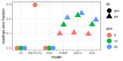
(a) Sparsity

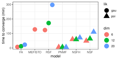
(b) Time to converge

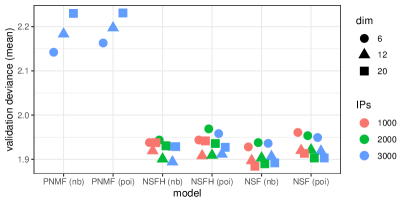
(c) Validation deviance by likelihood

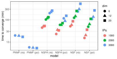
(d) Time to converge by likelihood

Figure S2: Benchmarking spatial and nonspatial factor models on Slide-seqV2 mouse hippocampus gene expression data. FA: factor analysis, RSF: real-valued spatial factorization, PNMF: probabilistic nonnegative matrix factorization, NSF: nonnegative spatial factorization, NSFH: NSF hybrid model, lik: likelihood, gau: Gaussian, poi: Poisson, nb: negative binomial. (a) Sparsity of loadings matrix increases with larger numbers of components (dim) in nonnegative models PNMF, NSFH, and NSF. (b) Nonnegative spatial models NSF and NSFH converge faster than MEFISTO but not as fast as nonspatial models FA and PNMF. (c) Negative binomial and Poisson likelihoods provide similar generalization accuracy (lower deviance) in nonnegative models. (d) Negative binomial likelihood is more computationally expensive than Poisson likelihood in nonnegative models.

In terms of sparsity, MEFISTO had the highest fraction of zero entries in the loadings matrix due to its sparsity promoting prior, followed by the nonnegative models NSFH, PNMF, and NSF (Figure S2a). Increasing the number of components also increased the sparsity. The time to convergence was comparable for all spatial models, with nonspatial models converging substantially faster (Figure S2b). Among nonnegative models, the negative binomial likelihood took longer to converge but did not reduce generalization error (Figure S2c-d). Both NSF and NSFH had similar deviances, suggesting that including a mixture of spatial and nonspatial components (NSFH) did not degrade generalization in comparison to a strictly spatial model (NSF).

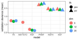
(a) Out-of-sample generalization error

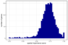
(b) Feature spatial importance

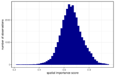
(c) Observation spatial importance

Figure 2: Benchmarking spatial and nonspatial factor models on Slide-seqV2 mouse hippocampus gene expression data. (a) Poisson deviance on held-out validation data. Lower deviance indicates better generalization accuracy. All spatial models used $2,000$ inducing points. lik: likelihood, dim: number of latent dimensions (components), FA: factor analysis, RSF: real-valued spatial factorization, PNMF: probabilistic nonnegative matrix factorization, NSF: nonnegative spatial factorization, NSFH: NSF hybrid model. (b) Each feature (gene) was assigned a spatial importance score derived from NSFH fit with $20$ components ($10$ spatial and $10$ nonspatial). A score of $1$ indicates spatial components explain all of the variation. (c) as (b) but with observations instead of features.

We examined the biological relevance of nonnegative factorization by focusing on the NSFH model with $M=3000$ inducing points and $L=20$ components ($10$ spatial and $10$ nonspatial). Each factor was summarized by its (variational) approximate posterior mean. For each spatial factor this is a function in the $(x,y)$ spatial coordinate system. For each nonspatial factor the posterior is a vector with one value per observation. Spatial importance scores indicate that most genes are strongly spatial, although a small number are entirely nonspatial (Figure 2b). At the observation level, spatial scores were less extreme, suggesting that both spatial and nonspatial factors are needed to explain gene expression at each location (Figure 2c).

Spatial factors mapped to specific brain regions (Figure 3a) such as the choroid plexus (1), medial habenula (6), and dentate gyrus (8). Even the thin meninges layer was distinguishable (10), underscoring the high spatial resolution of the Slide-seqV2 protocol. We identified genes with the highest enrichment to individual components by examining the loadings matrix. Spatial gene expression patterns mirrored the spatial factors to which they were most associated (Figure 3b). Nonspatial factors were generally dispersed across the field of view (Figure 3c). Finally, we used the top genes for each component to identify cell types and biological processes (Table 3) using scfind (Lee et al., 2021a) and the Panglao database (Franzén et al., 2019). For example, spatial component 5 identified the corpus callosum, a white-matter region where myelination is crucial. Similarly, the top cell type for spatial component 10 capturing the meninges layer was meningeal cells. Generally, neurons and glia were the most common cell types across all components.

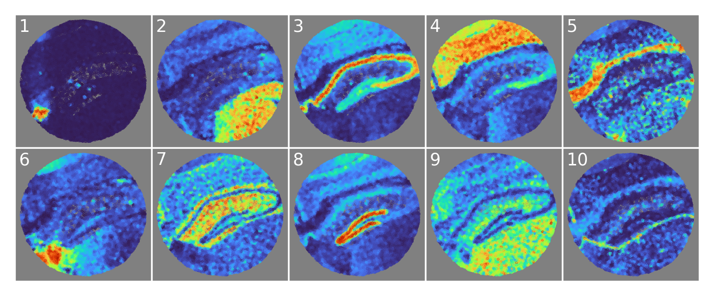
(a) NSFH spatial factors

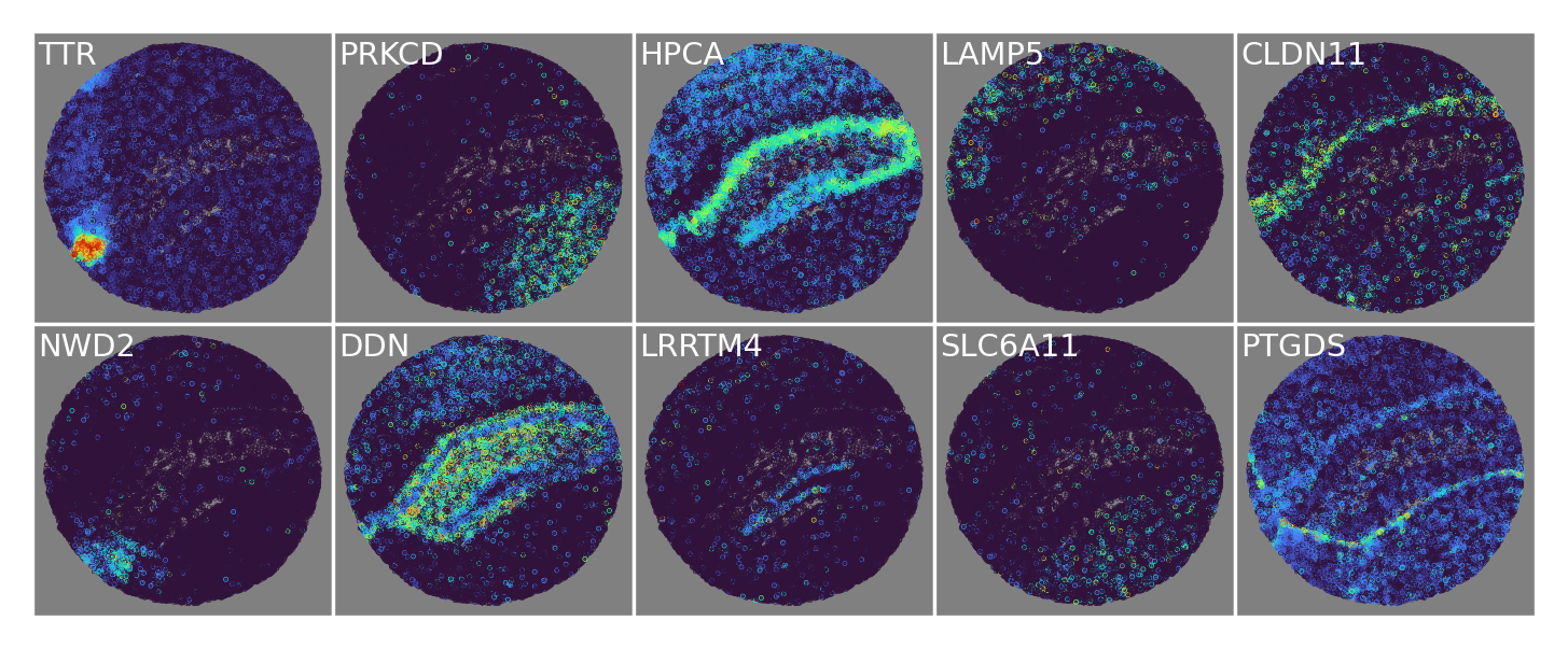
(b) NSFH spatially variable genes

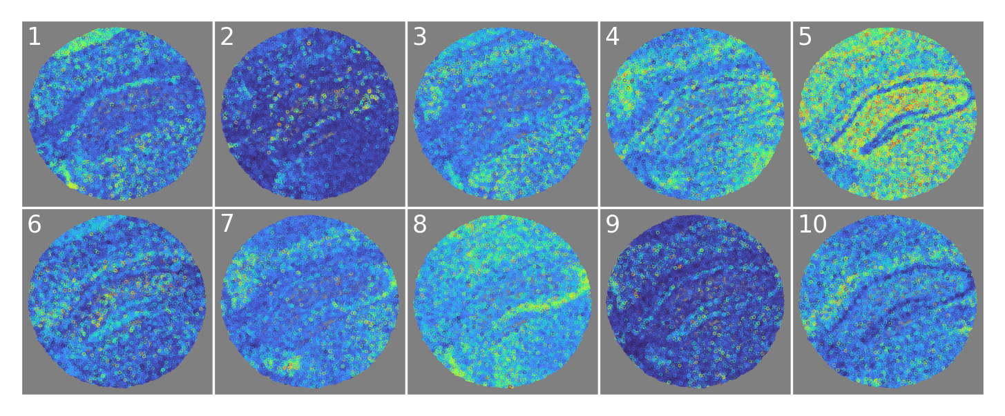
(c) NSFH nonspatial factors

Figure 3: Nonnegative spatial factorization hybrid model (NSFH) combines spatial and nonspatial factors in Slide-seqV2 mouse hippocampus gene expression data. Field-of-view is a coronal section with left indicating the medial direction and right the lateral direction. (a) Heatmap (red=high, blue=low) of square-root transformed posterior mean of $10$ spatial factors mapped into the $(x,y)$ coordinate space. (b) as (a) but mapping expression levels of top genes with strongest enrichment to each spatial component. (c) as (a) but mapping $10$ nonspatial factors from the same model.

Table 3: Nonnegative spatial factorization hybrid model (NSFH) identifies biologically distinct components in Slide-seqV2 mouse hippocampus.

dim	type	brain regions	cell types	genes	GO biological processes
1	spat	choroid plexus of third ventricle	Choroid plexus cells	TTR, ENPP2, IFI27, TRPM3, STK39	T cell migration, cellular response to chemokine
2	spat	thalamus	Interneurons	PRKCD, TNNT1, RAMP3, NTNG1, PDP1	regulation of presynaptic cytosolic calcium ion concentration, proteoglycan metabolic process
3	spat	CA1-3 (Ammon’s Horn) pyramidal layer	Neurons	HPCA, NEUROD6, CRYM, WIPF3, CPNE6	positive regulation of dendritic spine morphogenesis, postsynaptic modulation of chemical synaptic transmission
4	spat	cerebral cortex	Neurons	LAMP5, 3110035E14RIK, STX1A, MEF2C, EGR1	myeloid leukocyte differentiation, hormone biosynthetic process
5	spat	fiber tracts/ corpus callosum	Oligodendrocytes	CLDN11, MAL, MAG, PLP1, MOG	myelination, central nervous system myelination
6	spat	medial habenula (thalamus)	Neurons	NWD2, TAC2, CALB2, NECAB2, ZCCHC12	steroid biosynthetic process, sex differentiation
7	spat	CA strata and dentate gyrus molecular layer	Astrocytes	DDN, SLC1A3, CST3, PSD, CABP7	learning, response to amino acid
8	spat	dentate gyrus granule layer	Neurons	LRRTM4, STXBP6, SLC8A2, 2010300C02RIK, PLXNA4	central nervous system projection neuron axonogenesis, regulation of cytoskeleton organization
9	spat	multiple	Astrocytes	SLC6A11, SPARC, SLC4A4, KCNJ10, ATP1A2	negative regulation of blood coagulation, cellular amino acid catabolic process
10	spat	meninges	Meningeal cells	PTGDS, GFAP, APOD, FABP7, FXYD1	nitric oxide mediated signal transduction, epithelial cell proliferation
1	nsp		Neurons	MEG3, SNHG11, MIAT, CPNE7, TTC14	mRNA processing, RNA splicing
2	nsp		GABAergic neurons	SST, NPY, GAD2, GAD1, CNR1	neurotransmitter metabolic process, negative regulation of catecholamine secretion
3	nsp		Neurons	CHGA, RAB3C, HSPA4L, CKMT1, SYT4	chemical synaptic transmission, regulation of short-term neuronal synaptic plasticity
4	nsp		GABAergic neurons	PVALB, VAMP1, CPLX1, MT-ND1, SCRT1	mitochondrial respiratory chain complex I assembly, aerobic respiration
5	nsp		Astrocytes	MT-RNR2, MT-RNR1, 2900052N01RIK, MAP2, MT-ND5	electron transport coupled proton transport, response to nicotine
6	nsp		Astrocytes	GM3764, MALAT1, GPC5, LSAMP, TRPM3	cell adhesion, synaptic membrane adhesion
7	nsp		Neurons	NEFM, NEFH, MAP1B, VAMP1, SLC24A2	cell adhesion, intermediate filament cytoskeleton organization
8	nsp		Interneurons	NPTXR, SYN2, STMN2, NCALD, YWHAH	mitotic cell cycle, thyroid gland development
9	nsp		Neurons	NRG3, FGF14, CSMD1, DLG2, KCNIP4	social behavior, positive regulation of synapse assembly
10	nsp			MIR6236, LARS2, CMSS1, HEXB, CAMK1D	translation, positive regulation of signal transduction by p53 class mediator

2.3.2 XYZeq liver data

On the XYZeq mouse liver dataset, real-valued factor models again had lower validation deviance than nonnegative models and spatial models again outperformed their nonspatial analogs (Figure 2). The strictly spatial NSF model had slightly lower deviance than the hybrid spatial and nonspatial model NSFH.

(a) Out-of-sample generalization error

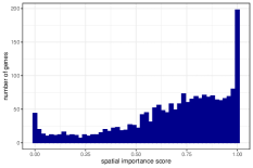
(b) Gene spatial importance

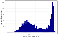
(c) Observation spatial importance

Figure 4: Benchmarking spatial and nonspatial factor models on XYZeq mouse liver gene expression data. Lower deviance indicates higher generalization accuracy. All spatial models used $288$ inducing points. lik: likelihood, dim: number of latent dimensions (components), FA: factor analysis, RSF: real-valued spatial factorization, PNMF: probabilistic nonnegative matrix factorization, NSF: nonnegative spatial factorization, NSFH: NSF hybrid model. (b) Each feature (gene) was assigned a spatial importance score derived from NSFH fit with $6$ components ($3$ spatial and $3$ nonspatial). A score of $1$ indicates spatial components explain all of the variation. (c) as (b) but with observations instead of features.

Focusing on the NSFH model with $M=288$ inducing points and $L=6$ components, we found a strikingly bimodal distribution of spatial importance scores for both genes and observations (Figure 4b-c). However, like the Slide-seqV2 data, most scores were greater than $0.5$, suggesting spatial variation was more explanatory than nonspatial overall. The first spatial factor identified normal liver tissue while the other spatial factors were associated with the tumor regions (Figure 5a). Genes associated with spatial component 1 indicated an enrichment of hepatocytes, while genes in the other components were associated with immune cells (Figure 5b, Table 4). The nonspatial factors again showed no distinct spatial patterns for these data (Figure 5c), although they were associated with particular cell types and biological processes (Table 4).

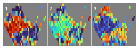
(a) NSFH spatial factors

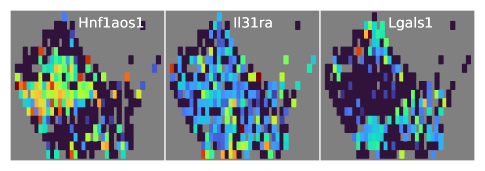
(b) NSFH spatially variable genes

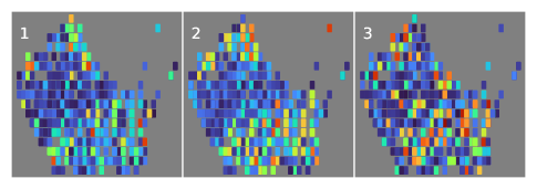
(c) NSFH nonspatial factors

Figure 5: Nonnegative spatial factorization hybrid model (NSFH) combines spatial and nonspatial factors in XYZeq mouse liver gene expression data. (a) Heatmap (red=high, blue=low) of square-root transformed posterior mean of $3$ spatial factors mapped into the $(x,y)$ coordinate space. (b) as (a) but mapping expression levels of top genes with strongest enrichment to each spatial component. (c) as (a) but mapping $3$ nonspatial factors from the same model.

Table 4: Nonnegative spatial factorization hybrid model (NSFH) identifies biologically distinct components in XYZeq mouse liver.

dim	type	cell types	genes	GO biological processes
1	spat	Hepatocytes	HNF1AOS1, CPS1, CYP2E1, AKR1C6, MUG2	cellular amino acid catabolic process, xenobiotic metabolic process
2	spat		IL31RA, SEMA5A, TRPM3, PLCD1, FOXP4	positive regulation of cholesterol esterification, inclusion body assembly
3	spat	Macrophages	LGALS1, S100A6, S100A4, RPL30, KLF6	translation, cytoplasmic translation
1	nsp	Fibroblasts	KIF26B, MEDAG, LAMA4, NGF, COL1A2	regulation of cellular response to vascular endothelial growth factor stimulus, collagen fibril organization
2	nsp		HMGA2, SLC35F1, FAM19A1, TENM4, HS3ST5	cell fate specification, specification of animal organ identity
3	nsp	Macrophages	ARHGAP15, DOCK10, MYO1F, LY86, HCK	negative regulation of leukocyte apoptotic process, negative regulation of immune response

2.3.3 Visium brain data

On the Visium mouse brain data, goodness-of-fit results in terms of validation deviance (lower values indicate better generalization accuracy) were markedly different than the other two datasets. First, real-valued models did not dominate nonnegative models. Both NSF and NSFH had lower deviance than factor analysis and MEFISTO. In fact, NSF had generalization accuracy comparable to the best-performing model (RSF). Furthermore, it was necessary to increase the number of components in NSFH to reduce the deviance to a level comparable with NSF, whereas in the other datasets deviance did not vary dramatically with the number of components, and NSFH had similar performance to NSF. However, consistent with the other datasets, nonspatial models generally had higher deviance than their spatial analogs, reinforcing the importance of including spatial information in out-of-sample prediction, interpolation, and generalization. Finally, the dramatic improvement in fit of RSF results over MEFISTO underscores the importance of choosing an appropriate GP kernel.

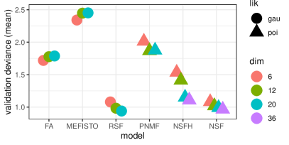
(a) Out-of-sample generalization error

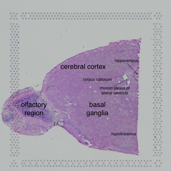
(b) Diagram of brain regions

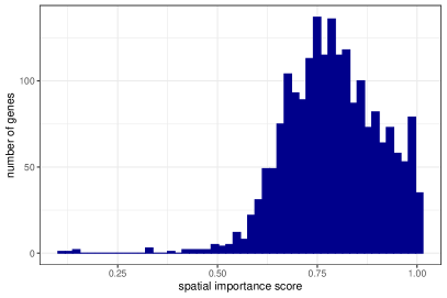
(c) Gene spatial importance

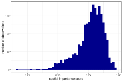
(d) Observation spatial importance

Figure 6: Benchmarking spatial and nonspatial factor models on Visium mouse brain gene expression data. Lower deviance indicates better generalization accuracy. All spatial models used $2,363$ inducing points. lik: likelihood, dim: number of latent dimensions (components), FA: factor analysis, RSF: real-valued spatial factorization, PNMF: probabilistic nonnegative matrix factorization, NSF: nonnegative spatial factorization, NSFH: NSF hybrid model. (b) Diagram of major brain regions, annotation by the authors, original image credit to 10x Genomics. (c) Each feature (gene) was assigned a spatial importance score derived from NSFH fit with $20$ components ($10$ spatial and $10$ nonspatial). A score of $1$ indicates spatial components explain all of the variation. (d) as (c) but with observations instead of features.

We next focused on interpretation of the NSFH model with $M=2363$ inducing points and $L=20$ components. A basic neuroanatomy diagram of mouse brain is provided for reference in Figure 6b. Spatial importance scores indicate that spatial factors are most explanatory for variation at both the gene and observation level (Figure 6c-d). Similar to the Slide-seqV2 data, most spatial factors mapped to specific brain regions (Figure 7a) such as the cerebral cortex (2), corpus callosum (4), and choroid plexus (10). Top genes for each spatial component again showed expression patterns overlapping with their associated factors (Figure 7b). While the majority of nonspatial factors were dispersed across the field-of-view (Figure 7c), a few of them did exhibit spatial localization to areas such as the hypothalamus (2) and hippocampus (4). This illustrates that the nonspatial factors are not antagonistic to spatial variation but should be thought of as spatially naive or agnostic. Given that Visium does not provide single-cell resolution, and this phenomenon was not observed in the other two datasets, we hypothesize that spatial patterns active in small numbers of observations may be more likely to be picked up as nonspatial factors under such conditions. Using the top genes for each component, we identified cell types and biological processes (Table 5). For example, spatial component 3 aligned to the basal ganglia, which is involved in the “response to amphetamine” biological process. Nonspatial component 10 had many genes associated with erythroid progenitor cells. The nonspatial patterns in this component suggest that this factor includes cell types in blood; however erythroid progenitor cells are not found in blood.. We hypothesize these are actually erythrocytes, which have been shown to retain parts of the erythroid transcriptome despite the loss of the nucleus (Doss et al., 2015). As in the Slide-seqV2 hippocampus data, neurons and glia were the most common cell types across all components.

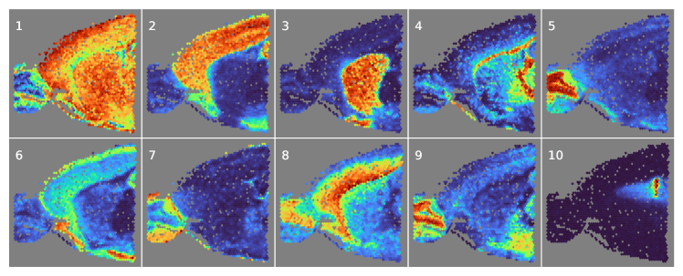
(a) NSFH spatial factors

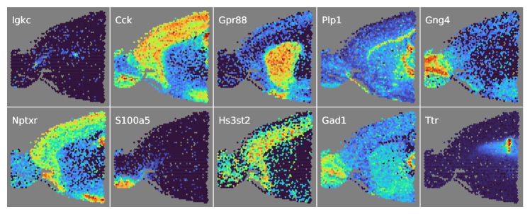
(b) NSFH spatially variable genes

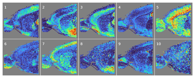
(c) NSFH nonspatial factors

Figure 7: Nonnegative spatial factorization hybrid model (NSFH) combines spatial and nonspatial factors in Visium mouse brain gene expression data. Field-of-view is a sagittal section with left indicating the anterior direction and right the posterior direction. (a) Heatmap (red=high, blue=low) of square-root transformed posterior mean of $10$ spatial factors mapped into the $(x,y)$ coordinate space. (b) as (a) but mapping expression levels of top genes with strongest enrichment to each spatial component. (c) as (a) but mapping $10$ nonspatial factors from the same model.

Table 5: Nonnegative spatial factorization hybrid model (NSFH) identifies biologically distinct components in Visium mouse brain.

dim	type	brain regions	cell types	genes	GO biological processes
1	spat	multiple		IGKC, COX6A2, TNNC1, CABP7, S100A9	mitochondrial electron transport, NADH to ubiquinone, mitochondrial respiratory chain complex I assembly
2	spat	cerebral cortex	Interneurons	CCK, DKK3, STX1A, NRN1, RTN4R	axonogenesis, positive regulation of behavioral fear response
3	spat	basal ganglia	Neurons	GPR88, PDE10A, RGS9, PPP1R1B, PENK	response to amphetamine, striatum development
4	spat	fiber tracts/ corpus callosum	Oligodendrocytes	PLP1, MAL, MOBP, MAG, CLDN11	myelination, central nervous system myelination
5	spat	olfactory granule layer	Neurons	GNG4, GPSM1, CPNE4, SHISA8, MYO16	embryonic limb morphogenesis, proximal/distal pattern formation
6	spat	multiple	Interneurons	NPTXR, CCN3, SLC30A3, RASL10A, LMO3	intracellular signal transduction, regulation of catalytic activity
7	spat	outer olfactory bulb	Interneurons	S100A5, DOC2G, CDHR1, CALB2, FABP7	mesoderm formation, cellular response to glucose stimulus
8	spat	inner cerebral cortex	Neurons	HS3ST2, IGHM, CCN2, IGSF21, NR4A2	isoprenoid biosynthetic process, cholesterol biosynthetic process
9	spat	multiple	GABAergic neurons	GAD1, SLC32A1, HAP1, STXBP6, CPNE7	neurotransmitter metabolic process, regulation of gamma-aminobutyric acid secretion
10	spat	choroid plexus of lateral ventricle	Choroid plexus cells	TTR, ECRG4, ENPP2, KL, 2900040C04RIK	hormone transport, retinol metabolic process
1	nsp		GABAergic neurons	PVALB, KCNAB3, CPLX1, VAMP1, SYT2	positive regulation of potassium ion transmembrane transporter activity, neuromuscular process
2	nsp	hypothalamus	Neurons	BAIAP3, NNAT, HPCAL1, LYPD1, RESP18	neurotrophin TRK receptor signaling pathway, muscle fiber development
3	nsp		Neurons	NEFM, LGI2, DNER, PLCXD2, CARTPT	regulation of synaptic vesicle fusion to presynaptic active zone membrane, neuronal action potential propagation
4	nsp	hippocampus	Neurons	WIPF3, CPNE6, RGS14, ARPC5, CABP7	Arp2/3 complex-mediated actin nucleation, calcineurin-NFAT signaling cascade
5	nsp		Neurons	HS3ST4, RAB26, CLSTN2, TLE4, SNCA	vacuolar acidification, protein glycosylation
6	nsp		Vascular fibroblasts	LARS2, GM42418, VTN, PTN, NPY	establishment of epithelial cell polarity, plasma lipoprotein particle organization
7	nsp		Neurons	PLXND1, VSTM2L, CALB1, RGS7, MGAT5B	heterophilic cell-cell adhesion via plasma membrane cell adhesion molecules, short-term memory
8	nsp		GABAergic neurons	SST, NPY, RESP18, NOS1, PDYN	neuropeptide signaling pathway, regulation of the force of heart contraction
9	nsp		Astrocytes	TUBB2B, GM3764, NTRK2, MFGE8, PLPP3	complement activation, negative regulation of growth
10	nsp		Erythrocytes	HBA-A1, HBA-A2, HBB-BT, HBB-BS, ALAS2	oxygen transport, cellular oxidant detoxification

3 Discussion

We have presented nonnegative spatial factorization (NSF), a probabilistic approach to spatially-aware dimension reduction on observations of count data based on Gaussian processes (GP). We also showed how to combine spatial and nonspatial factors with the NSF hybrid model (NSFH). On simulated data, NSF, NSFH, and the nonspatial model probabilistic NMF (PNMF) all recovered an interpretable parts-based representation, whereas real-valued factorizations such as MEFISTO (Velten et al., 2020) led to a less interpretable embedding. A key advantage of spatially-aware factorizations over unsupervised alternatives such as factor analysis (FA) and PNMF is generalizability; spatial factor models learn latent functions over the entire spatial domain rather than only at the observed locations. On a benchmarking task using three spatial transcriptomics (ST) datasets from three different technologies, NSF and NSFH had consistently lower out-of-sample prediction error than PNMF. We found that using a Matérn kernel reduced prediction error in our implementation of real-valued spatial factorization (RSF) when compared to MEFISTO, which uses a squared exponential kernel. We demonstrated how NSFH spatial and nonspatial components identify distinct regions in brain and liver tissue, cell types, and biological processes. Finally, we quantified the proportion of variation explained by spatial versus nonspatial components at both the gene and observation level using spatial importance scores.

A substantial limitation of the models studied here is the reliance on Euclidean distance as the metric for the GP kernel over the spatial domain. While this was appropriate for the particular datasets we explored, other ST datasets more closely resemble manifolds. An example is the embryonic tissue profiled by Lohoff et al. (2020). Under such conditions, standard GP kernels are inappropriate (Dunson et al., 2020). The recently proposed manifold GP (Borovitskiy et al., 2020) and graph GP (Borovitskiy et al., 2021) seem promising as alternatives. Either of these could be substituted for the standard GPs in our RSF, NSF, and NSFH models.

Historically, two major challenges for working with ST data have included integration with single-cell RNA-seq references (Lopez et al., 2019; Verma and Engelhardt, 2020) and deconvolving observations that incorporate multiple cells (Cable et al., 2021; Lopez et al., 2021). Addressing these will be an important future direction for research into nonnegative spatial factor models. However, we anticipate that ongoing improvements in ST protocols will increase the number of genes detected per location while improving the spatial resolution to single-cell or even subcellular levels (Eng et al., 2019; Xia et al., 2019) while maintaining a wide field-of-view.

All of the spatial models we considered were based on linear combinations of GPs with variational inference using inducing points (Leibfried et al., 2021; van der Wilk et al., 2020). While this technique has greatly improved GP scalability by enabling minibatching and nonconjugate likelihoods, the computational complexity still scales cubically with the number of inducing points. Promising future directions for GP inference include the harmonic kernel decomposition (Sun et al., 2021), nearest-neighbor GPs (Finley et al., 2019), and random Fourier features (Hensman et al., 2017; Gundersen et al., 2020). While linearity and nonnegativity are advantageous for interpretability (Svensson et al., 2020), multivariate spatial factor models can also be formulated using nonlinear deep GPs (Wu et al., 2021).

We have focused on the application of nonnegative spatial factor models to genomics data. However, both NSF and NSFH are relevant to other types of multivariate spatial or temporal data. Examples include forestry and environmental remote sensing (Taylor-Rodriguez et al., 2019), wearable devices (Straczkiewicz et al., 2021), and neuroscience (Wu et al., 2017; Foti and Fox, 2019).

4 Methods

4.1 Nonnegative spatial factorization inference

4.1.1 Evidence lower bound objective (ELBO) function

The posterior distribution of NSF cannot be computed in closed form, so we resort to approximate inference using a variational distribution. We assume a set of inducing point locations $z_{m}$ indexed by $m=1,\ldots,M$. If $M=N$ we set $z_{m}$ to be the spatial coordinates $X$. Otherwise, for $M<N$ we set $z_{m}$ to be the center points of a k-mean clustering (with $k=M$) applied to $X$. Let $u_{ml}=f_{l}(z_{m})$ be the inducing points, i.e., the Gaussian process evaluation of the inducing locations. We are interested in inference of the posterior of the latent variables $u_{ml}$ and $f_{il}$. Temporarily assume loadings $w_{jl}$, likelihood shape and dispersion parameters, GP prior mean parameters $\beta_{l}$, and kernel hyperparameters $\theta_{l}$ are known. The posterior is given by

$$p(U,F|~{}Y;~{}X,Z) =\frac{p(Y|~{}U,F)p(U,F;~{}X,Z)}{\int_{U,F}p(Y|~{}U,F)p(U,F;~{}X,Z)}$$

$$=\frac{p(Y|~{}F)p(F|~{}U;~{}X,Z)p(U;~{}Z)}{\int_{U,F}p(Y|~{}F)p(F|~{}U;~{}X,Z)p(U;~{}Z)}.$$

Note that the likelihood term depends on $U$ only through $F$, and we have decomposed the joint prior on $U,F$ into a marginal prior of $U$ and a conditional prior of $F|~{}U$. Following Salimbeni and Deisenroth (2017) and van der Wilk et al. (2020), the GP prior for inducing points is given by

$$p(U;~{}Z) =\prod_{l=1}^{L}p(\bm{u}_{l};~{}Z)$$

$$p(\bm{u}_{l};~{}Z) =\mathcal{N}\big{(}\mu_{l}(Z),~{}K_{uul}\big{)}$$

$$\big{[}K_{uul}\big{]}_{m,m^{\prime}} =k_{l}\big{(}\bm{z}_{m},\bm{z}_{m^{\prime}}).$$

Next, we specify the GP prior for the function values at the observed locations by conditioning on the inducing points.

$$p(F|~{}U;~{}X,Z) =\prod_{l=1}^{L}p(\bm{f}_{l}|~{}\bm{u}_{l};~{}X,Z)$$

$$p(\bm{f}_{l}|~{}\bm{u}_{l};~{}X,Z) =\mathcal{N}\big{(}\bm{\mu}_{f|~{}ul},~{}K_{f|~{}ul}\big{)}$$

$$\bm{\mu}_{f|~{}ul} =\mu_{l}(X)+K_{ufl}^{\prime}K_{uul}^{-1}\big{(}\bm{u}_{l}-\mu_{l}(Z)\big{)}$$

$$K_{f|~{}ul} =K_{ffl}-K_{ufl}^{\prime}K_{uul}^{-1}K_{ufl}$$

$$\big{[}K_{ufl}\big{]}_{m,i} =k_{l}(\bm{z}_{m},\bm{x}_{i})$$

$$\big{[}K_{ffl}\big{]}_{i,i^{\prime}} =k_{l}(\bm{x}_{i},\bm{x}_{i^{\prime}}).$$

Note that $K_{uul}\in\mathbb{R}^{M\times M}$, $K_{ffl}\in\mathbb{R}^{N\times N}$, and $K_{ufl}\in\mathbb{R}^{M\times N}$.

We use the following approximation to the true posterior to facilitate variational inference:

$$q(U,F;~{}X,Z) =p(F|~{}U;~{}X,Z)q(U;~{}Z)$$

$$q(U;~{}Z) =\prod_{l=1}^{L}q(\bm{u}_{l};~{}Z)$$

$$q(\bm{u}_{l};~{}Z) =\mathcal{N}\big{(}\bm{\delta}_{l},~{}\Omega_{l}\big{)}.$$

We will later need to draw samples of $F$ from this distribution. This is made easier by analytically marginalizing out $U$.

$$q(\bm{f}_{l}|~{}\bm{\delta}_{l},\Omega_{l};X,Z) =\int_{\bm{u}_{l}}p(\bm{f}_{l}|~{}\bm{u}_{l};~{}X,Z)q(\bm{u}_{l};~{}Z)$$

$$=\mathcal{N}\big{(}\tilde{\mu}_{l},~{}\tilde{\Sigma}_{l}),$$

where the marginal mean vector $\tilde{\mu}_{l}\in\mathbb{R}^{N}$ and covariance matrix $\tilde{\Sigma}_{l}\in\mathbb{R}^{N\times N}$ are given by

$$\tilde{\mu}_{l} =\mu_{l}(X)+K_{ufl}^{\prime}K_{uul}^{-1}\big{(}\bm{\delta}_{l}-\mu_{l}(Z)\big{)}$$

$$\tilde{\Sigma}_{l} =K_{ffl}-K_{ufl}^{\prime}K_{uul}^{-1}\big{(}K_{uul}-\Omega_{l}\big{)}K_{uul}^{-1}K_{ufl}.$$

Minimizing the KL divergence from the true posterior distribution to the approximating distribution is equivalent to maximizing the following evidence lower bound (ELBO) (Hensman et al., 2013; Salimbeni and Deisenroth, 2017; van der Wilk et al., 2020):

$$\mathcal{L} =\operatorname{\mbox{E}}_{q(U,F)}\left[\log\frac{p(Y|~{}F)p(F|~{}U;~{}X,Z)p(U;~{}Z)}{q(U,F)}\right]$$

$$=\operatorname{\mbox{E}}_{q(U,F)}\big{[}\log p(Y|~{}F)\big{]}+\operatorname{\mbox{E}}_{q(U,F)}\left[\log\frac{p(F|~{}U;~{}X,Z)p(U;~{}Z)}{p(F|~{}U;~{}X,Z)q(U;~{}Z)}\right]$$

$$=(\mathcal{L}_{1})-\sum_{l=1}^{L}\operatorname{\mbox{E}}_{q(\bm{u}_{l})}\left[\log\frac{q(\bm{u}_{l};~{}Z)}{p(\bm{u}_{l};~{}Z)}\right]$$

$$=\mathcal{L}_{1}-\sum_{l=1}^{L}\operatorname{KL}\big{(}q(\bm{u}_{l})~{}||~{}p(\bm{u}_{l})\big{)}.$$

The KL divergence term from prior to approximate posterior has a closed-form expression since both are Gaussian (recall $M$ is the total number of inducing points):

$$\operatorname{KL}\big{(}q(\bm{u}_{l})~{}||~{}p(\bm{u}_{l})\big{)} =\frac{1}{2}\left[\log\frac{|K_{uul}|}{|\Omega_{l}|}-M+\operatorname{tr}\big{\{}K_{uul}^{-1}\Omega_{l}\big{\}}+\big{(}\bm{\delta}_{l}-\mu_{l}(Z)\big{)}^{\prime}K_{uul}^{-1}\big{(}\bm{\delta}_{l}-\mu_{l}(Z)\big{)}\right].$$

Let $\zeta(y|~{}\nu\lambda)$ be the log likelihood of an exponential family such as the Poisson or negative binomial distribution with mean $\nu\lambda$. In particular, for the Poisson distribution, $\zeta(y|~{}\nu\lambda)=y\log(\nu\lambda)-\nu\lambda-\log y!$. Let $F[i,:]=(f_{i1},\ldots,f_{iL})$. The expected log likelihood term in the ELBO is given by:

$$\mathcal{L}_{1} =\sum_{i=1}^{N}\sum_{j=1}^{J}\operatorname{\mbox{E}}_{q(U,F)}\left[\zeta(y_{ij}|~{}\nu_{i}\lambda_{ij})\right]$$

$$=\sum_{i=1}^{N}\sum_{j=1}^{J}\operatorname{\mbox{E}}_{q(F)}\left[\zeta\left(y_{ij}\left|~{}\sum_{l=1}^{L}w_{jl}e^{f_{il}}\right.\right)\right]$$

$$=\sum_{i=1}^{N}\sum_{j=1}^{J}\operatorname{\mbox{E}}_{q(F[i,:])}\left[\zeta\left(y_{ij}\left|~{}\sum_{l=1}^{L}w_{jl}e^{f_{il}}\right.\right)\right].$$

The expectation in the above equation is intractable due to the nonlinear log likelihood function $\zeta(\cdot)$. However, we can simplify it in two ways. First, it only depends on $U$ through $F$, so the marginalized distribution $q(F)$ may be used instead of $q(U,F)$. Second, the log likelihood only depends on the marginal $f_{il}$ terms, as opposed to the multivariate $\bm{f}_{l}=(f_{1l},\ldots,f_{Nl})$ or the multivariate $F[i,:]$. The approximate posterior distribution is therefore $q(F[i,:])=\prod_{l=1}^{L}q(f_{il})=\prod_{l=1}^{L}\mathcal{N}\left(\left[\tilde{\mu}_{l}\right]_{i},~{}\left[\tilde{\Sigma}_{l}\right]_{i,i}\right)$, where

$$\alpha_{l}(\bm{x}_{i}) =K_{uul}^{-1}\big{[}K_{ufl}\big{]}_{:,i}$$

$$\left[\tilde{\mu}_{l}\right]_{i} =\mu_{l}(\bm{x}_{i})+\alpha_{l}(\bm{x}_{i})^{\prime}\big{(}\bm{\delta}_{l}-\mu_{l}(Z)\big{)}$$

$$\left[\tilde{\Sigma}_{l}\right]_{i,i} =k_{l}(\bm{x}_{i},\bm{x}_{i})-\alpha_{l}(\bm{x}_{i})^{\prime}\big{(}K_{uul}-\Omega_{l}\big{)}\alpha_{l}(\bm{x}_{i}).$$

Despite these simplifications, the expectation still lacks a closed-form solution and is evaluated by approximation using Monte Carlo (MC) sampling (Salimbeni and Deisenroth, 2017). The MC procedure draws $S$ samples $f^{(s)}_{il}\sim\mathcal{N}\left(\left[\tilde{\mu}_{l}\right]_{i},~{}\left[\tilde{\Sigma}_{l}\right]_{i,i}\right)$ then evaluates

$$\operatorname{\mbox{E}}_{q(F[i,:])}\left[\zeta\left(y_{ij}\left|~{}\sum_{l=1}^{L}w_{jl}e^{f_{il}}\right.\right)\right]\approx\frac{1}{S}\sum_{s=1}^{S}\left[\zeta\left(y_{ij}\left|~{}\sum_{l=1}^{L}w_{jl}e^{f^{(s)}_{il}}\right.\right)\right]$$

. In practice, we found $S=3$ to provide a reasonable balance between speed and numerical stability.

4.1.2 Parameter estimation

Using the ELBO as an objective function, we optimize all parameters using the Adam algorithm (Kingma and Ba, 2014) with gradients computed by automatic differentiation in Tensorflow (Abadi et al., 2016). This includes the loadings weights $w_{jl}$, mean function intercepts $\beta_{0l}$ and slopes $\bm{\beta}_{1l}$, kernel length scale and amplitude parameters, variational location $\bm{\delta}_{l}$ and covariance $\Omega_{l}$ parameters, and any shape or dispersion parameters associated with the likelihood (e.g., for negative binomial and Gaussian distributions).

To satisfy the nonnegativity constraint on $w_{jl}$, we use a projected gradient approach. After each optimization step, any values that are negative are truncated to zero. All other parameter constraints are accommodated by monotone transformations. For example, the variational covariance matrices $\Omega_{l}$ must all be positive definite, so we store and use the lower triangular Cholesky decomposition factors instead of the full covariance matrices themselves.

4.1.3 Real-valued spatial factorization inference

The inference procedure for RSF is identical to NSF except we do not exponentiate the sampled $f_{il}^{(s)}$ terms prior to combining with the loadings $w_{jl}$. Because the loadings are no longer constrained to be greater than or equal to zero, the truncation step is omitted during optimization. To facilitate comparisons with MEFISTO, we focused on a Gaussian likelihood and only applied RSF to normalized data with features centered to have zero mean.

4.2 Nonspatial count factorization inference

To fit PNMF and FA models, we adopt a mean field variational approximation (Blei et al., 2016) to the posterior distribution of the latent factors:

$$q(f_{il})=\mathcal{N}(\delta_{il},~{}\omega_{il})$$

. Focusing on PNMF, the ELBO is of the form

$$\mathcal{L} =\sum_{i=1}^{N}\sum_{j=1}^{J}\operatorname{\mbox{E}}_{q(F[i,:])}\left[\zeta\left(y_{ij}\left|~{}\sum_{l=1}^{L}w_{jl}e^{f_{il}}\right.\right)\right]-\sum_{i=1}^{N}\sum_{l=1}^{L}\operatorname{KL}\big{(}q(f_{il})~{}||~{}p(f_{il})\big{)}.$$

The expectation in the first term is approximated by MC sampling just as in NSF. The second term involves two univariate Gaussians and has the closed form

$$\operatorname{KL}\big{(}q(f_{il})~{}||~{}p(f_{il})\big{)} =\frac{1}{2}\left[\log\frac{s^{2}_{l}}{\omega_{il}}-1+\frac{\omega_{il}}{s^{2}_{l}}+\frac{(\delta_{il}-m_{l})^{2}}{s^{2}_{l}}\right].$$

FA has an identical setup to NSF except without exponentiating the sampled $f_{il}^{(s)}\sim q(f_{il})$. Optimization of parameters is the same as in NSF, including the truncation of $w_{jl}$ terms in PNMF.

4.3 Nonnegative spatial factorization hybrid (NSFH) model

Recall $\nu_{i}\lambda_{ij}$ is the mean of the outcome $y_{ij}$, which we assume is distributed as some exponential family likelihood, such as Gaussian, negative binomial, or Poisson. The NSFH model is specified as the combination of $T$ spatial factors with $L-T$ nonspatial factors

$$\lambda_{ij}=\sum_{l=1}^{T}w_{jl}e^{f_{il}}+\sum_{l=T+1}^{L}v_{jl}e^{h_{il}}.$$

To estimate the $f_{il}$ terms, we use the same GP prior and variational inducing point approximate posterior as in NSF. To estimate the $h_{il}$ terms, we use the same univariate Gaussian prior and mean field variational approximate posterior as in PNMF. The ELBO objective function is similar to NSF and PNMF:

$$\mathcal{L} =\sum_{i=1}^{N}\sum_{j=1}^{J}\operatorname{\mbox{E}}_{q(F[i,:],H[i,:])}\left[\zeta\left(y_{ij}\left|~{}\sum_{l=1}^{L}w_{jl}e^{f_{il}}+\sum_{l=T+1}^{L}v_{jl}e^{h_{il}}\right.\right)\right]\ldots$$

$$\ldots-\sum_{l=1}^{L}\operatorname{KL}\big{(}q(\bm{u}_{l})~{}||~{}p(\bm{u}_{l})\big{)}-\sum_{i=1}^{N}\sum_{l=1}^{L}\operatorname{KL}\big{(}q(h_{il})~{}||~{}p(h_{il})\big{)}.$$

Due to the mean-field formulation, the variational distributions factorize over components:

$$q(F[i,:],H[i,:])=\prod_{l=1}^{T}q(f_{il})\prod_{l=T+1}^{L}q(h_{il}).$$

Thus, we approximated the expectation by independent MC samples of $f_{il}^{(s)}\sim q(f_{il})$ and $h_{il}^{(s)}\sim q(h_{il})$. The remaining two KL divergence terms are identical to those in NSF and PNMF and have the same closed form. We optimize all parameters using the same techniques described for NSF and PNMF.

4.4 Postprocessing nonnegative factorizations

Consider a generic nonnegative factorization $\Lambda=FW^{\prime}$ or equivalently $\lambda_{ij}=\sum_{l}f_{il}w_{jl}$. We assume that the log-likelihood of data $Y$ depends on the $N\times L$ factors matrix $F$ and $J\times L$ loadings matrix $W$ only through $\Lambda$. The number of observations is $N$, number of components is $L$, and number of features is $J$. For notational simplicity, here we use $f_{il}$ to denote a nonnegative entry of a factor matrix rather than $e^{f_{il}}$ used in other sections. In the case that the model is probabilistic, we assume $f_{il}$ represents a posterior mean, posterior geometric mean, or other point estimate. We project $F,W$ onto the simplex while leaving the likelihood invariant.

$$\bar{f} =\sum_{i=1}^{N}F_{[i,:]}\in\mathbb{R}^{L}$$

$$F \leftarrow F*\operatorname{diag}(\bar{f})^{-1}$$

$$W \leftarrow W*\operatorname{diag}(\bar{f})$$

$$\bar{w} =\sum_{l=1}^{L}W_{[:,l]}\in\mathbb{R}^{J}$$

$$W \leftarrow\operatorname{diag}(\bar{w})^{-1}*W.$$

Note that after this transformation $\Lambda=FW^{\prime}\operatorname{diag}(\bar{w})$. We now have that the columns of $F$ all sum to one and the rows of $W$ all sum to one (i.e., they lie on the simplex). In the spatial transcriptomics context, the features are genes. A particular row of $W$ represents a single gene’s soft clustering assignment to each of the $L$ components. If $w_{jl}=1$ this meant all of that gene’s expression could be predicted using only component $l$, whereas if $w_{jl}=0$ this meant that component $l$ was irrelevant to gene $j$. For a given component $l$, we identified the top associated genes by sorting the $w_{jl}$ values in decreasing order.

We refer to the above procedure as “SPDE-style” postprocessing due to its similarity to spatialDE (Svensson et al., 2018). An alternative postprocessing scheme is “LDA-style” (Blei et al., 2003; Carbonetto et al., 2021) where the roles of $F$ and $W$ are switched. This results in a loadings matrix whose columns sum to one (“topics”) and a factors matrix whose rows sum to one. LDA-style postprocessing provides a soft clustering of observations instead of features. We used SPDE-style postprocessing throughout this work with the sole exception of computing spatial importance scores for observations, described below.

4.4.1 NSFH spatial importance scores

Let $F\in\mathbb{R}^{N\times T}_{+}$ represent the spatial factors matrix (rather than $e^{F}$), with corresponding loadings $W\in\mathbb{R}^{J\times T}_{+}$. Similarly let $H\in\mathbb{R}^{N\times(L-T)}_{+}$ represent the nonspatial factors (rather than $e^{H}$) with corresponding loadings $V\in\mathbb{R}^{J\times(L-T)}_{+}$. Let $A=[F,H]\in\mathbb{R}^{N\times L}_{+}$ and $B=[W,V]\in\mathbb{R}^{J\times L}_{+}$.

To obtain spatial importance scores for features (genes), we applied SPDE-style postprocessing to $A,B$. The score $\gamma_{j}$ for feature $j$ is given by the sum of the loadings weights across all the spatial components.

$$W\leftarrow B_{[:,1:T]}$$

$$\gamma_{j}=\sum_{l=1}^{T}w_{jl}.$$

Due to the initial postprocessing, $0\leq\gamma_{j}\leq 1$ for all $j$. If $\gamma_{j}=0$ then all the variation in feature $j$ was explained by the nonspatial factors. If $\gamma_{j}=1$ then all the variation was explained by the spatial factors.

To obtain spatial scores for observations, we applied LDA-style postprocessing to $A,B$. The score $\rho_{i}$ for observation $i$ is given by the sum of the factor values across all the spatial components.

$$F\leftarrow A_{[:,1:T]}$$

$$\rho_{i}=\sum_{l=1}^{T}f_{il}.$$

As before, $0\leq\rho_{i}\leq 1$ for all $i$. If $\rho_{i}=0$ then all the variation in observation $i$ was explained by the nonspatial factors. If $\rho_{i}=1$ then all the variation was explained by the spatial factors.

4.5 Initialization

Real-valued models were initialized with singular value decomposition. Nonnegative models were initialized with the scikit-learn implementation of NMF (Pedregosa et al., 2011). For NSFH, we sorted the initial NMF factors and loadings in decreasing order of spatial autocorrelation using Moran’s I statistic (Moran, 1950) as implemented in squidpy (Palla et al., 2021). The first $T$ factors were assigned to the spatial component and the remaining $L-T$ factors to the nonspatial component.

4.6 Simulations

In the ggblocks simulation, each latent factor representing a canonical spatial pattern consisted of a $30\times 30$ grid of locations ($900$ total spatial locations). The number of features (“genes”) was set to $500$. Each gene was randomly assigned to one of the four patterns with uniform probabilities. The $900\times 500$ mean matrix was defined as the sum of two nonnegative matrices: one spatial ($M_{1}$) and one nonspatial ($M_{2}$). Entries of $M_{1}$ were set to $11$ in the active region (where a shape is visible) and $0.1$ elsewhere. We then generated a set of three nonspatial factors each of length $900$ by drawing from a Bernoulli distribution with probability $0.2$. Each gene was randomly assigned to one of the three nonspatial factors with uniform probabilities. The entries of $M_{2}$ were then set to $9$ in active cells and $0.1$ elsewhere. The counts were then drawn from a negative binomial distribution with mean $M_{1}+M_{2}$ and shape parameter $10$ to promote overdispersion. For MEFISTO, RSF, and FA the count data were normalized to have the same total count at each spatial location, then log transformed with a pseudocount of one. Features were centered before applying each dimension reduction method. For PNMF, NSF, and NSFH the raw counts were used as input. The unsupervised methods (PNMF and FA) used only the $900\times 500$ count matrix, while the supervised methods (NSF, NSFH, RSF, and MEFISTO) also used the $900\times 2$ matrix of spatial coordinates. Since this was a smaller dataset, all spatial coordinates were used as inducing point locations to maximize accuracy. All models were fit with $L=4$ components, except NSFH which was fit with $L=7$ total components of which $T=4$ were spatial and the rest nonspatial.

For the quilt simulation, we followed the same procedure as above, but the spatial patterns were $36\times 36$, leading to $1296$ total observations, each at a unique spatial location.

4.7 Data acquisition and preprocessing

For all datasets, after quality control filtering of observations, we selected the top $2000$ informative genes using Poisson deviance as a criterion (Townes et al., 2019a; Street et al., 2021). Raw counts were used as input to nonnegative models (NSF, PNMF, NSFH) with size factors computed by the default Scanpy method as described below (Wolf et al., 2017). For real-valued models with Gaussian likelihoods (RSF, FA, MEFISTO), we followed the default Scanpy normalization for consistency with MEFISTO. The raw counts were normalized such that the total count per observation equaled the median of the total counts in the original data. The normalized counts were then log transformed with a pseudocount of one, and the features were centered to have mean zero. This scaled, log-normalized version of the data was then used for model fitting.

4.7.1 Visium mouse brain

The dataset “Mouse Brain Serial Section 1 (Sagittal-Anterior)“ was downloaded from https://support.10xgenomics.com/spatial-gene-expression/datasets. To facilitate comparisons, preprocessing followed the MEFISTO tutorial (https://nbviewer.jupyter.org/github/bioFAM/MEFISTO_tutorials/blob/master/MEFISTO_ST.ipynb) (Velten et al., 2020). Observations (spots) with total counts less than $100$ or mitochondrial counts greater than $20\%$ were excluded.

4.7.2 Slide-seqV2 mouse hippocampus

This dataset was originally produced by Stickels et al. (2021). We obtained it through the SeuratData R package (Satija et al., 2019) and converted it to a Scanpy H5AD file (Wolf et al., 2017) using SeuratDisk (Hoffman, 2021). Observations (spots) with total counts less than $100$ or mitochondrial counts greater than $20\%$ were excluded.

4.7.3 XYZeq mouse liver

This dataset was originally produced by Lee et al. (2021b). We obtained it from the Gene Expression Omnibus (Edgar et al., 2002), accession number GSE164430. We focused on sample liver_slice_L20C1, which was featured in the original publication, and downloaded it as an H5AD file. The spatial coordinates were provided by the original authors. We did not exclude any observations (cells), since all had total counts greater than $100$ and mitochondrial counts less than $20\%$.

4.8 Cell types and GO terms

For each dataset, we fit a NSFH model and applied SPDE-style postprocessing such that the loadings matrices had rows (representing genes) summing to one across all components. We then examined each column of the loadings matrix (representing a component) and identified the five genes with largest weights. We then manually searched for cell types on scfind (https://scfind.sanger.ac.uk/) (Lee et al., 2021a). If no results were found, we next searched the Panglao database (https://panglaodb.se) (Franzén et al., 2019). We identified brain regions in the Slide-seqV2 hippocampus and Visium brain datasets by referring to the interactive Allen Brain Atlas (https://atlas.brain-map.org) (Wang et al., 2020). GO annotations for all genes were downloaded from the BioMart ENSEMBL database (release 104, May 2021) using the biomaRt package in Bioconductor (version 3.13). Enriched terms were identified using the topGO Bioconductor package with the default algorithm “weight01” and statistic “fisher”, considering the top $100$ genes for each component against a background of all other genes.

4.9 Software versions and hardware

We implemented all models using Python 3.8.10, tensorflow 2.5.0, tensorflow probability 0.13.0. Other Python packages used include scanpy 1.8.0, squidpy 1.1.0, scikit-learn 0.24.2, pandas 1.2.5, numpy 1.19.5, scipy 1.7.0. We used the MEFISTO implementation from the mofapy2 Python package, installed from the GitHub development branch at commit 8f6ffcb5b18d22b3f44ff2a06bcb92f2806afed0. Graphics were generated using either matplotlib 3.4.2 in Python or ggplot2 3.3.5 (Wickham, 2016) in R (version 4.1.0). The R packages Seurat 0.4.3 (Hao et al., 2021), SeuratData 0.2.1, and SeuratDisk 0.0.0.9019 were used for some initial data manipulations. Computationally-intensive model fitting was done on Princeton’s Della cluster. Each model was assigned 12 CPU cores. We provided the following total memory per dataset: 180 Gb for Slide-seq V2, 72 Gb for Visium, and 48 Gb for XYZeq.

Code for reproducing the analyses of this manuscript is available from https://github.com/willtownes/nsf-paper.

Acknowledgments

The authors thank Britta Velten and the MEFISTO team for assistance in model fitting and responsiveness in bug fixes. George Hartoularos and Dylan Cable gave helpful advice on data acquisition and processing. Adelaide Minerva contributed expertise in neuroanatomy. Tina Townes helped with graphics. Anqi Wu and Stephen Keeley, along with members of the “BEEHIVE” including Archit Verma, Didong Li, Andy Jones and Siena Dumas Ang provided valuable insight through informal discussions. F.W.T. and B.E.E. were funded by a grant from the Helmsley Trust, a grant from the NIH Human Tumor Atlas Research Program, NIH NHLBI R01 HL133218, and NSF CAREER AWD1005627.

The work reported on in this paper relied on Princeton Research Computing resources at Princeton University, which is a consortium led by the Princeton Institute for Computational Science and Engineering (PICSciE) and the Office of Information Technology’s Research Computing.

Supplemental Figures

(a) ground truth

References

- Abadi et al. (2016) Martin Abadi, Paul Barham, Jianmin Chen, Zhifeng Chen, Andy Davis, Jeffrey Dean, Matthieu Devin, Sanjay Ghemawat, Geoffrey Irving, Michael Isard, Manjunath Kudlur, Josh Levenberg, Rajat Monga, Sherry Moore, Derek G. Murray, Benoit Steiner, Paul Tucker, Vijay Vasudevan, Pete Warden, Martin Wicke, Yuan Yu, and Xiaoqiang Zheng. TensorFlow: A System for Large-Scale Machine Learning. In Proceedings of the 12th USENIX Symposium on Operating Systems Design and Implementation, pages 265–283, 2016. ISBN 978-1-931971-33-1.
- Äijö et al. (2019) Tarmo Äijö, Silas Maniatis, Sanja Vickovic, Kristy Kang, Miguel Cuevas, Catherine Braine, Hemali Phatnani, Joakim Lundeberg, and Richard Bonneau. Splotch: Robust estimation of aligned spatial temporal gene expression data. bioRxiv, page 757096, September 2019. doi: 10.1101/757096.
- Banerjee et al. (2014) Sudipto Banerjee, Bradley P. Carlin, and Alan E. Gelfand. Hierarchical Modeling and Analysis for Spatial Data. CRC Press, September 2014. ISBN 978-1-4398-1918-0.
- Bartholomew et al. (2011) David J. Bartholomew, Martin Knott, and Irini Moustaki. Latent Variable Models and Factor Analysis: A Unified Approach. John Wiley & Sons, June 2011. ISBN 978-1-119-97370-6.
- BinTayyash et al. (2021) Nuha BinTayyash, Sokratia Georgaka, S. T. John, Sumon Ahmed, Alexis Boukouvalas, James Hensman, and Magnus Rattray. Non-parametric modelling of temporal and spatial counts data from RNA-seq experiments. bioRxiv, page 2020.07.29.227207, February 2021. doi: 10.1101/2020.07.29.227207.
- Blei et al. (2003) David M. Blei, Andrew Y. Ng, and Michael I. Jordan. Latent Dirichlet Allocation. J. Mach. Learn. Res., 3:993–1022, March 2003. ISSN 1532-4435.
- Blei et al. (2016) David M. Blei, Alp Kucukelbir, and Jon D. McAuliffe. Variational Inference: A Review for Statisticians. arXiv:1601.00670 [cs, stat], January 2016.
- Borovitskiy et al. (2020) Viacheslav Borovitskiy, Alexander Terenin, Peter Mostowsky, and Marc Peter Deisenroth. Mat\’ern Gaussian processes on Riemannian manifolds. arXiv:2006.10160 [cs, stat], October 2020.
- Borovitskiy et al. (2021) Viacheslav Borovitskiy, Iskander Azangulov, Alexander Terenin, Peter Mostowsky, Marc Deisenroth, and Nicolas Durrande. Matérn Gaussian Processes on Graphs. In International Conference on Artificial Intelligence and Statistics, pages 2593–2601. PMLR, March 2021.
- Butler et al. (2018) Andrew Butler, Paul Hoffman, Peter Smibert, Efthymia Papalexi, and Rahul Satija. Integrating single-cell transcriptomic data across different conditions, technologies, and species. Nature Biotechnology, April 2018. ISSN 1546-1696. doi: 10.1038/nbt.4096.
- Cable et al. (2021) Dylan M. Cable, Evan Murray, Luli S. Zou, Aleksandrina Goeva, Evan Z. Macosko, Fei Chen, and Rafael A. Irizarry. Robust decomposition of cell type mixtures in spatial transcriptomics. Nature Biotechnology, pages 1–10, February 2021. ISSN 1546-1696. doi: 10.1038/s41587-021-00830-w.
- Carbonetto et al. (2021) Peter Carbonetto, Abhishek Sarkar, Zihao Wang, and Matthew Stephens. Non-negative matrix factorization algorithms greatly improve topic model fits. arXiv:2105.13440 [cs, stat], May 2021.
- Cressie and Moores (2021) Noel Cressie and Matthew T. Moores. Spatial Statistics. arXiv:2105.07216 [stat], May 2021.
- Doss et al. (2015) Jennifer F. Doss, David L. Corcoran, Dereje D. Jima, Marilyn J. Telen, Sandeep S. Dave, and Jen-Tsan Chi. A comprehensive joint analysis of the long and short RNA transcriptomes of human erythrocytes. BMC Genomics, 16(1):952, November 2015. ISSN 1471-2164. doi: 10.1186/s12864-015-2156-2.
- Dries et al. (2021) Ruben Dries, Qian Zhu, Rui Dong, Chee-Huat Linus Eng, Huipeng Li, Kan Liu, Yuntian Fu, Tianxiao Zhao, Arpan Sarkar, Feng Bao, Rani E. George, Nico Pierson, Long Cai, and Guo-Cheng Yuan. Giotto: A toolbox for integrative analysis and visualization of spatial expression data. Genome Biology, 22(1):78, March 2021. ISSN 1474-760X. doi: 10.1186/s13059-021-02286-2.
- Dunson et al. (2020) David B. Dunson, Hau-Tieng Wu, and Nan Wu. Diffusion Based Gaussian Processes on Restricted Domains. arXiv:2010.07242 [math, stat], October 2020.
- Edgar et al. (2002) Ron Edgar, Michael Domrachev, and Alex E. Lash. Gene Expression Omnibus: NCBI gene expression and hybridization array data repository. Nucleic Acids Research, 30(1):207–210, January 2002. ISSN 0305-1048, 1362-4962. doi: 10.1093/nar/30.1.207.
- Editors (2021) Editors. Method of the Year 2020: Spatially resolved transcriptomics. Nature Methods, 18(1):1–1, January 2021. ISSN 1548-7105. doi: 10.1038/s41592-020-01042-x.
- Elyanow et al. (2020) Rebecca Elyanow, Bianca Dumitrascu, Barbara E. Engelhardt, and Benjamin J. Raphael. netNMF-sc: Leveraging gene-gene interactions for imputation and dimensionality reduction in single-cell expression analysis. Genome Research, page gr.251603.119, January 2020. ISSN 1088-9051, 1549-5469. doi: 10.1101/gr.251603.119.
- Eng et al. (2019) Chee-Huat Linus Eng, Michael Lawson, Qian Zhu, Ruben Dries, Noushin Koulena, Yodai Takei, Jina Yun, Christopher Cronin, Christoph Karp, Guo-Cheng Yuan, and Long Cai. Transcriptome-scale super-resolved imaging in tissues by RNA seqFISH+. Nature, 568(7751):235–239, April 2019. ISSN 1476-4687. doi: 10.1038/s41586-019-1049-y.
- Finley et al. (2019) Andrew O. Finley, Abhirup Datta, Bruce D. Cook, Douglas C. Morton, Hans E. Andersen, and Sudipto Banerjee. Efficient Algorithms for Bayesian Nearest Neighbor Gaussian Processes. Journal of Computational and Graphical Statistics, 28(2):401–414, April 2019. ISSN 1061-8600. doi: 10.1080/10618600.2018.1537924.
- Foti and Fox (2019) Nicholas J Foti and Emily B Fox. Statistical model-based approaches for functional connectivity analysis of neuroimaging data. Current Opinion in Neurobiology, 55:48–54, April 2019. ISSN 0959-4388. doi: 10.1016/j.conb.2019.01.009.
- Franzén et al. (2019) Oscar Franzén, Li-Ming Gan, and Johan L M Björkegren. PanglaoDB: A web server for exploration of mouse and human single-cell RNA sequencing data. Database, 2019(baz046), January 2019. ISSN 1758-0463. doi: 10.1093/database/baz046.
- Gelfand et al. (2004) Alan E. Gelfand, Alexandra M. Schmidt, Sudipto Banerjee, and C. F. Sirmans. Nonstationary multivariate process modeling through spatially varying coregionalization. Test, 13(2):263–312, December 2004. ISSN 1863-8260. doi: 10.1007/BF02595775.
- Griffiths and Ghahramani (2011) Thomas L. Griffiths and Zoubin Ghahramani. The Indian Buffet Process: An Introduction and Review. Journal of Machine Learning Research, 12(Apr):1185–1224, 2011. ISSN ISSN 1533-7928.
- Gundersen et al. (2020) Gregory W. Gundersen, Michael Minyi Zhang, and Barbara E. Engelhardt. Latent variable modeling with random features. arXiv:2006.11145 [cs, stat], June 2020.
- Hao et al. (2021) Yuhan Hao, Stephanie Hao, Erica Andersen-Nissen, William M. Mauck, Shiwei Zheng, Andrew Butler, Maddie J. Lee, Aaron J. Wilk, Charlotte Darby, Michael Zager, Paul Hoffman, Marlon Stoeckius, Efthymia Papalexi, Eleni P. Mimitou, Jaison Jain, Avi Srivastava, Tim Stuart, Lamar M. Fleming, Bertrand Yeung, Angela J. Rogers, Juliana M. McElrath, Catherine A. Blish, Raphael Gottardo, Peter Smibert, and Rahul Satija. Integrated analysis of multimodal single-cell data. Cell, 184(13):3573–3587.e29, June 2021. ISSN 0092-8674, 1097-4172. doi: 10.1016/j.cell.2021.04.048.
- Hensman et al. (2013) James Hensman, Nicolo Fusi, and Neil D. Lawrence. Gaussian Processes for Big Data. arXiv:1309.6835 [cs, stat], September 2013.
- Hensman et al. (2017) James Hensman, Nicolas Durrande, and Arno Solin. Variational Fourier features for Gaussian processes. The Journal of Machine Learning Research, 18(1):5537–5588, January 2017. ISSN 1532-4435.
- Hicks et al. (2018) Stephanie C. Hicks, F. William Townes, Mingxiang Teng, and Rafael A. Irizarry. Missing data and technical variability in single-cell RNA-sequencing experiments. Biostatistics, 19(4):562–578, October 2018. ISSN 1465-4644. doi: 10.1093/biostatistics/kxx053.
- Hoffman (2021) Paul Hoffman. SeuratDisk: Interfaces for HDF5-Based single cell file formats, 2021.
- Hotelling (1933) H. Hotelling. Analysis of a complex of statistical variables into principal components. Journal of Educational Psychology, 24(6):417–441, 1933. ISSN 1939-2176(Electronic),0022-0663(Print). doi: 10.1037/h0071325.
- Huggins et al. (2017) Jonathan Huggins, Ryan P Adams, and Tamara Broderick. PASS-GLM: Polynomial approximate sufficient statistics for scalable Bayesian GLM inference. In I. Guyon, U. V. Luxburg, S. Bengio, H. Wallach, R. Fergus, S. Vishwanathan, and R. Garnett, editors, Advances in Neural Information Processing Systems 30, pages 3611–3621. Curran Associates, Inc., 2017.
- Jones et al. (2021) Andrew Jones, F. William Townes, Didong Li, and Barbara E. Engelhardt. Contrastive latent variable modeling with application to case-control sequencing experiments. arXiv:2102.06731 [q-bio, stat], February 2021.
- Keeley et al. (2020) Stephen Keeley, David Zoltowski, Yiyi Yu, Spencer Smith, and Jonathan Pillow. Efficient Non-conjugate Gaussian Process Factor Models for Spike Count Data using Polynomial Approximations. In International Conference on Machine Learning, pages 5177–5186. PMLR, November 2020.
- Kim et al. (2020) Tae Kim, Xiang Zhou, and Mengjie Chen. Demystifying “drop-outs” in single cell UMI data. bioRxiv, page 2020.03.31.018911, April 2020. doi: 10.1101/2020.03.31.018911.
- Kingma and Ba (2014) Diederik Kingma and Jimmy Ba. Adam: A Method for Stochastic Optimization. arXiv:1412.6980 [cs], December 2014.
- Lee and Seung (1999) Daniel D. Lee and H. Sebastian Seung. Learning the parts of objects by non-negative matrix factorization. Nature, 401(6755):788–791, October 1999. ISSN 0028-0836. doi: 10.1038/44565.
- Lee et al. (2021a) Jimmy Tsz Hang Lee, Nikolaos Patikas, Vladimir Yu Kiselev, and Martin Hemberg. Fast searches of large collections of single-cell data using scfind. Nature Methods, 18(3):262–271, March 2021a. ISSN 1548-7105. doi: 10.1038/s41592-021-01076-9.
- Lee et al. (2021b) Youjin Lee, Derek Bogdanoff, Yutong Wang, George C. Hartoularos, Jonathan M. Woo, Cody T. Mowery, Hunter M. Nisonoff, David S. Lee, Yang Sun, James Lee, Sadaf Mehdizadeh, Joshua Cantlon, Eric Shifrut, David N. Ngyuen, Theodore L. Roth, Yun S. Song, Alexander Marson, Eric D. Chow, and Chun Jimmie Ye. XYZeq: Spatially resolved single-cell RNA sequencing reveals expression heterogeneity in the tumor microenvironment. Science Advances, 7(17):eabg4755, April 2021b. ISSN 2375-2548. doi: 10.1126/sciadv.abg4755.
- Leibfried et al. (2021) Felix Leibfried, Vincent Dutordoir, S. T. John, and Nicolas Durrande. A Tutorial on Sparse Gaussian Processes and Variational Inference. arXiv:2012.13962 [cs, stat], February 2021.
- Lohoff et al. (2020) T. Lohoff, S. Ghazanfar, A. Missarova, N. Koulena, N. Pierson, J. A. Griffiths, E. S. Bardot, C.-H. L. Eng, R. C. V. Tyser, R. Argelaguet, C. Guibentif, S. Srinivas, J. Briscoe, B. D. Simons, A.-K. Hadjantonakis, B. Göttgens, W. Reik, J. Nichols, L. Cai, and J. C. Marioni. Highly multiplexed spatially resolved gene expression profiling of mouse organogenesis. bioRxiv, page 2020.11.20.391896, November 2020. doi: 10.1101/2020.11.20.391896.
- Lopez et al. (2018) Romain Lopez, Jeffrey Regier, Michael B. Cole, Michael I. Jordan, and Nir Yosef. Deep generative modeling for single-cell transcriptomics. Nature Methods, 15(12):1053–1058, December 2018. ISSN 1548-7105. doi: 10.1038/s41592-018-0229-2.
- Lopez et al. (2019) Romain Lopez, Achille Nazaret, Maxime Langevin, Jules Samaran, Jeffrey Regier, Michael I. Jordan, and Nir Yosef. A joint model of unpaired data from scRNA-seq and spatial transcriptomics for imputing missing gene expression measurements. arXiv:1905.02269 [cs, q-bio, stat], May 2019.
- Lopez et al. (2021) Romain Lopez, Baoguo Li, Hadas Keren-Shaul, Pierre Boyeau, Merav Kedmi, David Pilzer, Adam Jelinski, Eyal David, Allon Wagner, Yoseph Addadi, Michael I. Jordan, Ido Amit, and Nir Yosef. Multi-resolution deconvolution of spatial transcriptomics data reveals continuous patterns of inflammation. bioRxiv, page 2021.05.10.443517, May 2021. doi: 10.1101/2021.05.10.443517.
- Matthews et al. (2017) Alexander G. de G. Matthews, Mark van der Wilk, Tom Nickson, Keisuke Fujii, Alexis Boukouvalas, Pablo Le{\’o}n-Villagr{\’a}, Zoubin Ghahramani, and James Hensman. GPflow: A Gaussian Process Library using TensorFlow. Journal of Machine Learning Research, 18(40):1–6, 2017. ISSN 1533-7928.
- Maynard et al. (2021) Kristen R. Maynard, Leonardo Collado-Torres, Lukas M. Weber, Cedric Uytingco, Brianna K. Barry, Stephen R. Williams, Joseph L. Catallini, Matthew N. Tran, Zachary Besich, Madhavi Tippani, Jennifer Chew, Yifeng Yin, Joel E. Kleinman, Thomas M. Hyde, Nikhil Rao, Stephanie C. Hicks, Keri Martinowich, and Andrew E. Jaffe. Transcriptome-scale spatial gene expression in the human dorsolateral prefrontal cortex. Nature Neuroscience, pages 1–12, February 2021. ISSN 1546-1726. doi: 10.1038/s41593-020-00787-0.
- Moran (1950) P. A. P. Moran. Notes on Continuous Stochastic Phenomena. Biometrika, 37(1/2):17–23, 1950. ISSN 0006-3444. doi: 10.2307/2332142.
- Moses and Pachter (2021) Lambda Moses and Lior Pachter. Museum of Spatial Transcriptomics. bioRxiv, page 2021.05.11.443152, May 2021. doi: 10.1101/2021.05.11.443152.
- Palla et al. (2021) Giovanni Palla, Hannah Spitzer, Michal Klein, David Sebastian Fischer, Anna Christina Schaar, Louis Benedikt Kuemmerle, Sergei Rybakov, Ignacio L. Ibarra, Olle Holmberg, Isaac Virshup, Mohammad Lotfollahi, Sabrina Richter, and Fabian J. Theis. Squidpy: A scalable framework for spatial single cell analysis. bioRxiv, page 2021.02.19.431994, February 2021. doi: 10.1101/2021.02.19.431994.
- Pedregosa et al. (2011) Fabian Pedregosa, Gaël Varoquaux, Alexandre Gramfort, Vincent Michel, Bertrand Thirion, Olivier Grisel, Mathieu Blondel, Peter Prettenhofer, Ron Weiss, Vincent Dubourg, Jake Vanderplas, Alexandre Passos, David Cournapeau, Matthieu Brucher, Matthieu Perrot, and Édouard Duchesnay. Scikit-learn: Machine Learning in Python. Journal of Machine Learning Research, 12(85):2825–2830, 2011.
- Rasmussen and Williams (2005) Carl Edward Rasmussen and Christopher K. I. Williams. Gaussian Processes for Machine Learning. MIT Press, November 2005.
- Salimbeni and Deisenroth (2017) Hugh Salimbeni and Marc Deisenroth. Doubly stochastic variational inference for deep Gaussian processes. In Advances in Neural Information Processing Systems, pages 4588–4599, 2017.
- Sarkar and Stephens (2020) Abhishek K. Sarkar and Matthew Stephens. Separating measurement and expression models clarifies confusion in single cell RNA-seq analysis. bioRxiv, page 2020.04.07.030007, April 2020. doi: 10.1101/2020.04.07.030007.
- Satija et al. (2019) Rahul Satija, Paul Hoffman, and Andrew Butler. SeuratData: Install and manage seurat datasets, 2019.
- Sherman et al. (2020) Thomas D. Sherman, Tiger Gao, and Elana J. Fertig. CoGAPS 3: Bayesian non-negative matrix factorization for single-cell analysis with asynchronous updates and sparse data structures. BMC Bioinformatics, 21(1):453, October 2020. ISSN 1471-2105. doi: 10.1186/s12859-020-03796-9.
- Stephenson et al. (2021) William T. Stephenson, Soumya Ghosh, Tin D. Nguyen, Mikhail Yurochkin, Sameer K. Deshpande, and Tamara Broderick. Measuring the sensitivity of Gaussian processes to kernel choice. arXiv:2106.06510 [cs, stat], June 2021.
- Stickels et al. (2021) Robert R. Stickels, Evan Murray, Pawan Kumar, Jilong Li, Jamie L. Marshall, Daniela J. Di Bella, Paola Arlotta, Evan Z. Macosko, and Fei Chen. Highly sensitive spatial transcriptomics at near-cellular resolution with Slide-seqV2. Nature Biotechnology, 39(3):313–319, March 2021. ISSN 1546-1696. doi: 10.1038/s41587-020-0739-1.
- Straczkiewicz et al. (2021) Marcin Straczkiewicz, Peter James, and Jukka-Pekka Onnela. A systematic review of smartphone-based human activity recognition for health research. arXiv:1910.03970 [cs, q-bio], March 2021.
- Street et al. (2021) Kelly Street, F. William Townes, Davide Risso, and Stephanie Hicks. Scry: Small-count analysis methods for high-dimensional data, 2021.
- Sun et al. (2021) Shengyang Sun, Jiaxin Shi, Andrew Gordon Wilson, and Roger Grosse. Scalable Variational Gaussian Processes via Harmonic Kernel Decomposition. arXiv:2106.05992 [cs, stat], June 2021.
- Sun et al. (2019) Shiquan Sun, Jiaqiang Zhu, Ying Ma, and Xiang Zhou. Accuracy, robustness and scalability of dimensionality reduction methods for single-cell RNA-seq analysis. Genome Biology, 20(1):269, December 2019. ISSN 1474-760X. doi: 10.1186/s13059-019-1898-6.
- Svensson (2020) Valentine Svensson. Droplet scRNA-seq is not zero-inflated. Nature Biotechnology, pages 1–4, January 2020. ISSN 1546-1696. doi: 10.1038/s41587-019-0379-5.
- Svensson et al. (2018) Valentine Svensson, Sarah A. Teichmann, and Oliver Stegle. SpatialDE: Identification of spatially variable genes. Nature Methods, 15(5):343–346, May 2018. ISSN 1548-7105. doi: 10.1038/nmeth.4636.
- Svensson et al. (2020) Valentine Svensson, Adam Gayoso, Nir Yosef, and Lior Pachter. Interpretable factor models of single-cell RNA-seq via variational autoencoders. Bioinformatics, 2020. doi: 10.1093/bioinformatics/btaa169.
- Taylor-Rodriguez et al. (2019) Daniel Taylor-Rodriguez, Andrew O. Finley, Abhirup Datta, Chad Babcock, Hans-Erik Andersen, Bruce D. Cook, Douglas C. Morton, and Sudipto Banerjee. Spatial Factor Models for High-Dimensional and Large Spatial Data: An Application in Forest Variable Mapping. Statistica Sinica, 29:1155–1180, 2019. ISSN 1017-0405. doi: 10.5705/ss.202018.0005.
- Townes et al. (2019a) F. William Townes, Stephanie C. Hicks, Martin J. Aryee, and Rafael A. Irizarry. Feature selection and dimension reduction for single-cell RNA-Seq based on a multinomial model. Genome Biology, 20(1):295, December 2019a. ISSN 1474-760X. doi: 10.1186/s13059-019-1861-6.
- Townes et al. (2019b) F. William Townes, Kelly Street, and Jake Yeung. Glmpca: Dimension Reduction of Non-Normally Distributed Data, September 2019b.
- van der Wilk et al. (2020) Mark van der Wilk, Vincent Dutordoir, S. T. John, Artem Artemev, Vincent Adam, and James Hensman. A Framework for Interdomain and Multioutput Gaussian Processes. arXiv:2003.01115 [cs, stat], March 2020.
- Velten et al. (2020) Britta Velten, Jana Muriel Braunger, Damien Arnol, Ricard Argelaguet, and Oliver Stegle. Identifying temporal and spatial patterns of variation from multi-modal data using MEFISTO. bioRxiv, page 2020.11.03.366674, November 2020. doi: 10.1101/2020.11.03.366674.
- Verma and Engelhardt (2020) Archit Verma and Barbara Engelhardt. A Bayesian nonparametric semi-supervised model for integration of multiple single-cell experiments. bioRxiv, page 2020.01.14.906313, January 2020. doi: 10.1101/2020.01.14.906313.
- Verma et al. (2021) Archit Verma, Siddhartha G. Jena, Danielle R. Isakov, Kazuhiro Aoki, Jared E. Toettcher, and Barbara E. Engelhardt. A self-exciting point process to study multicellular spatial signaling patterns. Proceedings of the National Academy of Sciences, 118(32), August 2021. ISSN 0027-8424, 1091-6490. doi: 10.1073/pnas.2026123118.
- Vickovic et al. (2019) Sanja Vickovic, Gökcen Eraslan, Fredrik Salmén, Johanna Klughammer, Linnea Stenbeck, Denis Schapiro, Tarmo Äijö, Richard Bonneau, Ludvig Bergenstråhle, José Fernandéz Navarro, Joshua Gould, Gabriel K. Griffin, Åke Borg, Mostafa Ronaghi, Jonas Frisén, Joakim Lundeberg, Aviv Regev, and Patrik L. Ståhl. High-definition spatial transcriptomics for in situ tissue profiling. Nature Methods, pages 1–4, September 2019. ISSN 1548-7105. doi: 10.1038/s41592-019-0548-y.
- Wang et al. (2020) Quanxin Wang, Song-Lin Ding, Yang Li, Josh Royall, David Feng, Phil Lesnar, Nile Graddis, Maitham Naeemi, Benjamin Facer, Anh Ho, Tim Dolbeare, Brandon Blanchard, Nick Dee, Wayne Wakeman, Karla E. Hirokawa, Aaron Szafer, Susan M. Sunkin, Seung Wook Oh, Amy Bernard, John W. Phillips, Michael Hawrylycz, Christof Koch, Hongkui Zeng, Julie A. Harris, and Lydia Ng. The Allen Mouse Brain Common Coordinate Framework: A 3D Reference Atlas. Cell, 181(4):936–953.e20, May 2020. ISSN 0092-8674. doi: 10.1016/j.cell.2020.04.007.
- Wickham (2016) Hadley Wickham. Ggplot2: Elegant Graphics for Data Analysis. Springer-Verlag New York, 2016. ISBN 978-3-319-24277-4.
- Wolf et al. (2017) F. Alexander Wolf, Philipp Angerer, and Fabian J. Theis. Scanpy for analysis of large-scale single-cell gene expression data. bioRxiv, page 174029, August 2017. doi: 10.1101/174029.
- Wu et al. (2017) Anqi Wu, Nicholas A. Roy, Stephen Keeley, and Jonathan W Pillow. Gaussian process based nonlinear latent structure discovery in multivariate spike train data. In I. Guyon, U. V. Luxburg, S. Bengio, H. Wallach, R. Fergus, S. Vishwanathan, and R. Garnett, editors, Advances in Neural Information Processing Systems 30, pages 3496–3505. Curran Associates, Inc., 2017.
- Wu et al. (2021) Anqi Wu, Samuel A. Nastase, Christopher A. Baldassano, Nicholas B. Turk-Browne, Kenneth A. Norman, Barbara E. Engelhardt, and Jonathan W. Pillow. Brain kernel: A new spatial covariance function for fMRI data. bioRxiv, page 2021.03.22.436524, March 2021. doi: 10.1101/2021.03.22.436524.
- Xia et al. (2019) Chenglong Xia, Jean Fan, George Emanuel, Junjie Hao, and Xiaowei Zhuang. Spatial transcriptome profiling by MERFISH reveals subcellular RNA compartmentalization and cell cycle-dependent gene expression. Proceedings of the National Academy of Sciences, 116(39):19490–19499, September 2019. ISSN 0027-8424, 1091-6490. doi: 10.1073/pnas.1912459116.
- Yu et al. (2009) Byron M Yu, John P Cunningham, Gopal Santhanam, Stephen I. Ryu, Krishna V Shenoy, and Maneesh Sahani. Gaussian-process factor analysis for low-dimensional single-trial analysis of neural population activity. In D. Koller, D. Schuurmans, Y. Bengio, and L. Bottou, editors, Advances in Neural Information Processing Systems 21, pages 1881–1888. Curran Associates, Inc., 2009.
- Zeira et al. (2021) Ron Zeira, Max Land, and Benjamin J. Raphael. Alignment and Integration of Spatial Transcriptomics Data. bioRxiv, page 2021.03.16.435604, March 2021. doi: 10.1101/2021.03.16.435604.
- Zhao and Park (2017) Yuan Zhao and Il Memming Park. Variational Latent Gaussian Process for Recovering Single-Trial Dynamics from Population Spike Trains. Neural Computation, 29(5):1293–1316, March 2017. ISSN 0899-7667. doi: 10.1162/NECO˙a˙00953.