A fast time domain solver for the equilibrium Dyson equation

Abstract

We consider the numerical solution of the real time equilibrium Dyson equation, which is used in calculations of the dynamical properties of quantum many-body systems. We show that this equation can be written as a system of coupled, nonlinear, convolutional Volterra integro-differential equations, for which the kernel depends self-consistently on the solution. As is typical in the numerical solution of Volterra-type equations, the computational bottleneck is the quadratic-scaling cost of history integration. However, the structure of the nonlinear Volterra integral operator precludes the use of standard fast algorithms. We propose a quasilinear-scaling FFT-based algorithm which respects the structure of the nonlinear integral operator. The resulting method can reach large propagation times, and is thus well-suited to explore quantum many-body phenomena at low energy scales. We demonstrate the solver with two standard model systems: the Bethe graph, and the Sachdev-Ye-Kitaev model.

Keywords — nonlinear Volterra integral equations, fast algorithms, equilibrium Dyson equation, many-body Green’s function methods

1 Introduction

Quantum many-body systems [1, 2, 3] can be described in terms of many-body Green’s functions, which characterize the system’s response to the addition and removal of one or more particles at different points in time. The number of degrees of freedom required to describe a many-body Green’s function scales polynomially with the system size, independently of the number of particles. Green’s function methods therefore provide an important complement to wavefunction-based methods, especially for macroscopic systems, since the dimensionality of a wavefunction is proportional to the number of particles it describes. A large number of physical properties can be determined just from single particle Green’s functions, which give the expectation value associated with the addition and removal of a single particle.

The equation of motion for the single particle Green’s function is called the Dyson equation [1]. The static thermal equilibrium properties of quantum many-body systems can be obtained by solving the equation of motion in imaginary time [3], and the dynamical properties by solving it in real time or frequency. The last decade has seen a revival of time domain Green’s function methods [4], mainly driven by an interest in non-equilibrium phenomena. This has in turn spurred advances in the development of numerical algorithms both for imaginary time [5, 6, 7, 8, 9, 10, 11, 12, 13, 14, 15, 16] and non-equilibrum real time [17, 18, 19, 20, 21, 22] Green’s functions. However, the real time Dyson equation can also be used to determine the dynamical properties of quantum many-body systems in equilibrium, by evolving the imaginary time Green’s function along the real time axis.

As we will show in Section 3.2, the Dyson equation of motion for the equilibrium single particle Green’s function in real time can be written as a system of coupled nonlinear Volterra integro-differential equations of the form

$$\begin{cases}&iy^{\prime}(t)+\int_{0}^{t}k\left(y(t-t^{\prime}),t-t^{\prime}\right)y(t^{\prime})\,dt^{\prime}=f(y(t),t)\\ &y(0)=y_{0}.\end{cases}$$ (1)

In that context, the solution $y$ is a real time single particle Green’s function, and the interaction kernel $k$ is called the self-energy. For simplicity of exposition, we take all quantities to be complex scalar-valued, but the matrix-valued case often encountered in Green’s function calculations is a straightforward generalization. We also note that although we have assumed local nonlinearities $k(t)=k(y(t),t)$ and $f(t)=f(y(t),t)$, our method applies equally well to the more general case of causal nonlinearities $k(t)=k(y(t^{\prime})|_{t^{\prime}\leq t},t)$ and $f(t)=f(y(t^{\prime})|_{t^{\prime}\leq t},t)$, which appear in more complicated diagrammatic models of the self-energy.

The cost of computing the history integral term in (1) scales as $\mathcal{O}\left(N^{2}\right)$ with the number $N$ of time steps, severely limiting the propagation times achievable by time domain solvers [23]. This creates a practical barrier in studies of collective low energy phenomena in quantum many-body systems, which require high resolution in the frequency domain. This approach is typically avoided as a result. The standard alternative is to evaluate the self-energy in the time domain, where it is typically simpler, and transform to the frequency domain to solve the Dyson equation and obtain the corresponding Green’s function. While this method eliminates the problem of history integration, and can be accelerated using the fast Fourier transform (FFT) [24], it requires solving a global nonlinear problem [25, 26]. The convergence properties of a given nonlinear iteration procedure are problem dependent, and the number of iterations can grow in physically interesting regimes, such as the low temperature limit.

We also mention another method, which is to perform analytic continuation to obtain a simpler integral equation in the imaginary time domain, and then analytically continue the solution back to the real time or frequency domain by solving a severely ill-conditioned integral equation [27]. For sufficiently complicated approximations to the self-energy, direct solution in real time or frequency can be impractical, and this technique is the only option. However, despite significant recent progress in sophisticated regularization methods [28, 29, 30], the analytic continuation problem is fundamentally ill-posed, and obtaining high quantitative accuracy reliably, as we seek here, remains a challenge.

In this work, we present a time stepping algorithm for (1) which reduces the cost of Volterra history integration to $\mathcal{O}\left(N\log^{2}N\right)$, eliminating the main barrier to carrying out equilibrium Green’s function calculations in the time domain. Using this approach, the nonlinear problem is local and well-controlled; the number of nonlinear iterations is independent of global features of the solution, and is typically very small. In combination with the recently introduced discrete Lehmann representation [16] of the imaginary time axis, our time domain algorithm enables the calculation of dynamical properties of quantum many-body systems at low temperatures and large propagation times, i.e. at low energy scales, which are essential in capturing emergent many-body excitations.

The problem of efficient Volterra history integration is well known in the scientific computing literature, and several techniques have been proposed, particularly in the context of solving Volterra integral equations and computing nonlocal transparent boundary conditions. We mention fast Fourier transform (FFT)-based methods [31], methods based on sum-of-exponentials projections of the history [32, 33, 34, 35, 36, 37, 38, 39, 40], convolution quadrature [41, 42], and hierarchical low-rank or butterfly matrix compression [22, 43, 44]. Of the methods mentioned above, several have been applied to the efficient numerical solution of convolutional nonlinear Volterra integral equations [31, 42, 43]. However, we emphasize that the form of the nonlinearity in (1) is different from that typically considered,

$$\int_{0}^{t}k(t-t^{\prime})F\left(y(t^{\prime}),t^{\prime}\right)\,dt^{\prime},$$ (2)

where $k$, or its Laplace transform, is given either explicitly or numerically. All of the methods cited above make use of this a priori access to $k$ in order to obtain a fast history summation scheme, and are therefore not applicable in the present setting, in which $k$ itself is determined during the course of time stepping by a self-consistency condition. This can be made evident by considering a simple example, $k(y(t),t)=y(t)$, which yields the integral operator $\int_{0}^{t}y(t-t^{\prime})y(t^{\prime})\,dt^{\prime}$ in (1). We refer to the form of the nonlinearity considered here as a kernel nonlinearity, to distinguish it from nonlinearities of the form (2).

Our algorithm is inspired by the FFT-based method of Hairer, Lubich, and Schlichte (HLS), proposed for the numerical solution of Volterra integral equations with nonlinearities of the typical form (2) [31]. Their approach, which will be discussed in detail in Section 2.1, is to restructure the history sums into a hierarchy of Toeplitz block matrix-vector products, and to apply the blocks in quasi-linear time using the FFT. This yields an $\mathcal{O}\left(N\log^{2}N\right)$ algorithm. Although their method does not apply directly to the present case because of the kernel nonlinearity, we find that a more sophisticated block partitioning gives a compatible algorithm with the same computational complexity.

This paper is organized as follows. We begin in Section 2 by describing our fast algorithm to compute the history integrals in (1). In Section 3, we give a brief introduction to many-body Green’s functions and the equilibrium Dyson equation for single particle Green’s functions, and show that the latter can be reduced to a system of coupled equations of the form (1). In Section 4, we apply our method to two canonical model systems: the Bethe graph [45, 46] and the Sachdev-Yitaev-Ke (SYK) model [47, 48, 49]. We demonstrate a significant increase in attainable propagation times, and therefore improvements in the resolution of the fine spectral properties of solutions. A concluding discussion is given in Section 5. We also provide appendices describing a specific high-order time stepping method for (1), and technical algorithmic details of the proposed method.

2 Fast history summation

To illustrate the appearance of the history sums in a simple manner, we first write down a forward Euler discretization of (1). We do not recommend using this method in practice, due to its poor accuracy and stability properties. Rather, we propose a high-order implicit multistep method in Appendix A. History sums of the same form appear no matter the choice of discretization, and the details of our fast history summation algorithm are independent of this choice.

Applying the forward Euler method to (1) yields

$$y_{n+1}=y_{n}+i\Delta t\int_{0}^{t_{n}}k(t_{n}-t^{\prime})y(t^{\prime})\,dt^{\prime}-i\Delta tf_{n}.$$

Here $t_{n}=n\Delta t$ for a time step $\Delta t$ and $n=0,\ldots,N-1$, $y_{n}\approx y(t_{n})$, and $f_{n}=f(t_{n})$. For notational simplicity, we have suppressed the dependence of $k$ and $f$ on $y$. Applying the trapezoidal rule to the integral gives

$$y_{n+1}=y_{n}+i\Delta t^{2}\sum_{m=0}^{n}k_{n-m}y_{m}-\frac{i\Delta t^{2}}{2}\left(k_{n}y_{0}+k_{0}y_{n}\right)-i\Delta tf_{n}.$$

The computational bottleneck is evidently the calculation of the history sum

$$s_{n}=\sum_{m=0}^{n}k_{n-m}y_{m}$$ (3)

at each time step. Indeed, the cost to compute all history sums for $n=0,\ldots,N-1$ is $\mathcal{O}\left(N^{2}\right)$, and dominates the otherwise $\mathcal{O}\left(N\right)$ cost of time stepping.

The collection of history sums takes the form of a lower triangular Toeplitz matrix-vector product $s=Ky$. Here, $s,y\in\mathbb{C}^{N}$ and $K\in\mathbb{C}^{N\times N}$, with $K_{nm}=k_{n-m}$ for $n\geq m$ and $K_{nm}=0$ for $n<m$, $n,m=0,\ldots,N-1$. An $N\times N$ Toeplitz matrix can be applied to a vector in $\mathcal{O}\left(N\log N\right)$ operations using the FFT; a detailed description of the algorithm is given in Appendix B. Therefore, if $y$ and $k$ were known, then computing the sums (3) with quasi-linear cost would be straightforward.

However, in the present setting, there are two additional complications:

1. $y_{n}$ must be computed in order to obtain $s_{n}$, which must in turn be computed in order to obtain $y_{n+1}$.

2. $y_{n}$ must be computed in order to obtain $k_{n}$, which must in turn be computed in order to obtain $y_{n+1}$.

The first, which is familiar in the literature on fast algorithms for Volterra-type equations and integral operators, prevents us from computing the history sums all at once as a matrix-vector product, so we cannot simply use the standard algorithm for the fast application of Toeplitz matrices. The HLS algorithm [31], which we review in Section 2.1, offers a solution to this problem, as do the many other methods for the efficient evaluation of Volterra integral operators mentioned in the introduction. The second problem has not, to our knowledge, been addressed in this literature. We will propose a solution in Section 2.2, which appropriately modifies the HLS algorithm to respect the causal structure of the kernel nonlinearity.

2.1 HLS algorithm for fast history summation with a fixed kernel

The HLS algorithm computes the sums (3), for the case in which the kernel $k$ is known, in $\mathcal{O}\left(N\log^{2}N\right)$ operations [31]. The matrix $K_{nm}=k_{n-m}$ is partitioned into square blocks as in Figure 1. In particular, we define $n_{j}=\lceil jN/2^{L}\rceil$ for $j=1,\ldots,2^{L}-1$ and $n_{2^{L}}=N-1$, where $L$ is the number of levels of subdivision. We choose $L=\mathcal{O}\left(\log_{2}N\right)$ so that $n_{1}$ is a small, fixed constant. Each block is Toeplitz, and therefore can be applied with quasi-optimal complexity using the FFT.

Figure 1: Illustration of the HLS algorithm to compute the history sums (3) on the fly with a given kernel $k$. Here, we have $L=3$ levels. The lettered blocks correspond to entries which are incorporated into the partial sums by direct summation, and the numbered blocks are applied using a fast Toeplitz matrix-vector product. The blocks are processed in the order corresponding to their first row indices: a-1-b-2-c-3-d-4-e-5-f-6-g-7-h.

The algorithm proceeds by accumulating partial sums $\widetilde{s}_{n}$ in an efficient manner, such that by the $n$th time step, $\widetilde{s}_{n}=s_{n}$ as needed. Contributions to the partial sums come both from triangular blocks (shown as the lettered blocks in Figure 1) applied directly row-by-row, and square blocks (shown as the numbered blocks in Figure 1) applied using the FFT. The algorithm amounts to a re-ordering of the calculation of history sums from the standard row-by-row approach, so as to enable the use of the FFT.

A pseudocode is given in Algorithm 1. We note the use of colon notation for indexing into vectors; for a vector $x$, we define $x_{i:j}\equiv(x_{i},\ldots,x_{j})^{T}$. Let us go through the first few steps of the algorithm.

1:Given: The first and last row indices, $r_{j}^{f}$ and $r_{j}^{l}$, and the first and last column indices, $c_{j}^{f}$ and $c_{j}^{l}$, of block $j$ in Figure 1, for $j=1,\ldots,2^{L}-1$

2:Initialize $\widetilde{s}_{0:N-1}=0$

3:for $n=0,n_{1}-1$ do

4:     $s_{n}\leftarrow\sum_{m=0}^{n}k_{n-m}y_{m}$

5:     Take a time step to obtain $y_{n+1}$

6:end for

7:for $j=1,2^{L}-1$ do

8:     Apply block $j$ to $y_{c_{j}^{f}:c_{j}^{l}}$ using FFT-based algorithm, and add result to $\widetilde{s}_{r_{j}^{f}:r_{j}^{l}}$

9:     for $n=n_{j},n_{j+1}-1$ do

10:         Compute local contribution to history sums: $\widetilde{s}_{n}\leftarrow\widetilde{s}_{n}+\sum_{m=n_{j}+1}^{n}k_{n-m}y_{m}$

11:         Set $s_{n}=\widetilde{s}_{n}$ and take a time step to obtain $y_{n+1}$

12:     end for

13:end for

Algorithm 1 Time-stepping using the HLS algorithm

First, the time steps $n=0,\ldots,n_{1}-1$ are carried out by the standard method, with the history sums $s_{0},\ldots,s_{n_{1}-1}$ computed by direct summation. Once $y_{n_{1}}$ has been computed, block 1 in Figure 1 can be applied to the vector $y_{0:n_{1}}$, yielding partial contributions to the sums $s_{n_{1}:n_{2}-1}$. These partial contributions are stored in $\widetilde{s}_{n_{1}:n_{2}-1}$.

Next, we carry out time steps $n=n_{1}$ to $n=n_{2}-1$. At the $n$th time step, we add the local contribution corresponding to the $n$th row of block b to the stored partial sum $\widetilde{s_{n}}$: $\widetilde{s}_{n}\leftarrow\widetilde{s}_{n}+\sum_{m=n_{1}+1}^{n}k_{n-m}y_{m}$. We then take $s_{n}=\widetilde{s}_{n}$, and can compute $y_{n+1}$.

Once $y_{n_{2}}$ has been obtained, block 2 can be applied to $y_{0:n_{2}}$, and the result stored in $\widetilde{s}_{n_{2}:n_{4}-1}$. Then we proceed with time steps $n=n_{2}$ to $n=n_{3}-1$. At the $n$th time step, we add the local contribution corresponding to the $n$th row of block c to $\widetilde{s}_{n}$, $\widetilde{s}_{n}\leftarrow\widetilde{s}_{n}+\sum_{m=n_{2}+1}^{n}k_{n-m}y_{m}$, set $s_{n}=\widetilde{s}_{n}$, and obtain $y_{n+1}$.

Once $y_{n_{3}}$ is obtained, block 3 can be applied to $y_{n_{2}+1:n_{3}}$, and its contribution added to $\widetilde{s}_{n_{3}:n_{4}-1}$. Then the local contributions corresponding to the rows of block d are added to the partial sums in order to take the corresponding time steps. The algorithm proceeds in this manner, with contributions from each block added to the corresponding partial sums in the indicated order, such that by the end of the $n$th time step, $\widetilde{s_{n}}=s_{n}$ as needed.

To derive the computational complexity of this algorithm, we simply add up the cost of applying all blocks. Recall that $L=\mathcal{O}\left(log_{2}N\right)$. Since each triangular block is of dimensional approximately $N/2^{L}=\mathcal{O}\left(1\right)$, and there are $2^{L}=\mathcal{O}\left(N\right)$ such blocks, the total cost of applying these blocks is $\mathcal{O}\left(N\right)$. For the square blocks, we have one block of dimension approximately $N/2$, two blocks of dimension $N/4$, four blocks of dimension $N/8$, and so on. The total cost of applying these blocks using the fast Toeplitz algorithm is therefore approximately

$$\sum_{l=1}^{L}2^{l-1}\times\frac{N}{2^{l}}\log\left(\frac{N}{2^{l}}\right)=\mathcal{O}\left(N\log^{2}N\right).$$

2.2 Fast history summation with a kernel nonlinearity

The HLS algorithm cannot be applied if $k_{n+1},\ldots,k_{N-1}$ are unknown at the $n$th time step. Indeed, the block $j$ is applied as soon as $y_{n_{j}}$ is obtained. However, block $j$ may contain values $k_{n}$ of the kernel with $k>n_{j}$; for example, block $4$ contains values up to $k_{N-1}$. Since $k_{n}$ depends on $y_{n}$, it is not possible to apply the full blocks in the order prescribed by the algorithm. In particular, only the upper triangular parts of blocks 1, 2, and 4 are known at the step they must be applied.

A modified partitioning of the same matrix is depicted in Figure 2. It contains square, triangular, and parallelogram-shaped blocks. In Appendix B, we generalize the standard FFT-based algorithm for Toeplitz matrices to triangular and parallelogram-shaped blocks (appropriately completed to full rectangular matrices by zero-padding), allowing these blocks to be applied in $\mathcal{O}\left(n\log n\right)$ operations as well.

Figure 2: Modification of the block structure depicted in Figure 1 to account for kernels which are obtained on the fly. The blocks are again processed in the order corresponding to their first row indices: a-1-b-2-c-3-d-4-e-5-f-6-g-7-h. Blocks with the same label and subscripts $1$ and $2$, like $3_{1}$ and $3_{2}$, can be processed simultaneously.

The structure of our algorithm is similar to that of the HLS algorithm, but with the modified partitioning. The triangular blocks indicated in Figure 2 by letters contain rows which are applied directly, and the numbered blocks are applied as soon as the time step corresponding to their first row $n_{j}$ is reached. The shapes of the numbered blocks ensure that their entries depend only on $k_{n}$ for $n\leq n_{j}$. The results of both the direct and block applications are accumulated in partial sums $\widetilde{s}_{n}$ as before. Unlike in the HLS algorithm, at each time step there are two local contributions that must be made; the first, as before, corresponds to values $y_{m}$ for $m$ near the current time step $n$, and the second to values $k_{m}$ for $m$ near $n$. Also, at some steps, two blocks are applied instead of one. A pseudocode for the full procedure is given in Algorithm 2. The partioning for $L=5$ is shown in Figure 3. This is similar to Figure 2, but contains more levels.

1:Given: The first and last row indices, $r_{j}^{f}$ and $r_{j}^{l}$, and the first and last column indices, $c_{j}^{f}$ and $c_{j}^{l}$, of block $j$ in Figure 1, for $j=1,2,3_{1},3_{2},4,5_{1},5_{2},\ldots$

2:Initialize $\widetilde{s}_{0:N-1}=0$

3:for $n=0,n_{1}-1$ do

4:     $s_{n}\leftarrow\sum_{m=0}^{n}k_{n-m}y_{m}$

5:     Take a time step to obtain $y_{n+1}$

6:end for

7:for $j=1,2^{L}-1$ do

8:     if there is one numbered block at row $n_{j}$ then

9:         Apply block $j$ to $y_{c_{j}^{f}:c_{j}^{l}}$ using FFT-based algorithm, and add result to $\widetilde{s}_{r_{j}^{f}:r_{j}^{l}}$

10:     else

11:         There are two blocks at row $n_{j}$; do the same as above, for $j=j_{1}$ and $j=j_{2}$

12:     end if

13:     for $n=n_{j},n_{j+1}-1$ do

14:         Compute local contribution to history sums: $\widetilde{s}_{n}\leftarrow\widetilde{s}_{n}+\sum_{m=0}^{n-n_{j}-1}k_{n-m}y_{m}+\sum_{m=n_{j}+1}^{n}k_{n-m}y_{m}$

15:         Set $s_{n}=\widetilde{s}_{n}$ and take a time step to obtain $y_{n+1}$

16:     end for

17:end for

Algorithm 2 Time-stepping using the fast history summation algorithm for kernel nonlinearities

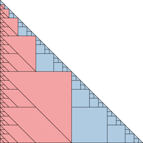
Figure 3: Illustration of the block partitioning of the kernel matrix for the full fast algorithm, with $L=5$. The full partioning is comprised of triangular units (blue) from the HLS algorithm (Figure 1), and square units (red), which account for the self-consistent nature of (1).

To obtain the computational complexity of the new algorithm, we consider the two types of units separately. We know from the previous section that the total cost of applying the triangular HLS-type units, indicated in blue in Figure 3, is approximately

$$\sum_{l=1}^{L}\frac{N}{2^{l}}\log^{2}\left(\frac{N}{2^{l}}\right)=\mathcal{O}\left(N\log^{2}N\right).$$

The total cost of applying each block in the square unit of dimension $N/2^{l}$ is

$$\frac{N}{2^{l}}\log\left(\frac{N}{2^{l}}\right)+\sum_{k=0}^{L-l}2^{k}\frac{N}{2^{l+k}}\log\left(\frac{N}{2^{l+k}}\right)\\ \leq\frac{N}{2^{l}}\log\left(\frac{N}{2^{l}}\right)(L-l+2).$$

Here, the first term corresponds to the top-right upper triangular block, and the second term corresponds to the rest of the blocks. Summing over all square units gives the total cost

$$\sum_{l=1}^{L}\left(\frac{N}{2^{l}}\log\left(\frac{N}{2^{l}}\right)(L-l+2)\right)=\mathcal{O}\left(N\log^{2}N\right).$$

Thus the computational complexity of the modified algorithm is $\mathcal{O}\left(N\log^{2}N\right)$, the same as that of the original HLS algorithm.

3 Green’s functions and the equilibrium Dyson equation

The aim of this section is to give a brief introduction to quantum many-body theory, the single particle Green’s function, and the Dyson equation of motion, starting from basic quantum mechanics. We refer the reader to [4] for a more thorough introduction to the subject.

In thermal equilibrium, the state of a quantum many-body system is described by a many-body density matrix $\hat{\varrho}$, which represents a statistical mixture of states $\ket{\psi_{n}}$ weighted, according to the Gibbs distribution, by $e^{-\beta E_{n}}/Z$:

$$\hat{\varrho}=\frac{e^{-\beta\hat{H}}}{Z}=\frac{1}{Z}\sum_{n}e^{-\beta E_{n}}|\psi_{n}\rangle\langle\psi_{n}|.$$

Here $\hat{H}$ is the Hamiltonian of the system for times $t<0$, $\beta$ is the inverse temperature, $|\psi_{n}\rangle$ is an eigenstate of the system with energy $E_{n}$, $\hat{H}|\psi_{n}\rangle=E_{n}|\psi_{n}\rangle$, and $Z$ is the partition function $Z=\sum_{n}e^{-\beta E_{n}}$.

In this context, the expectation value of an operator $\hat{O}$ is given by the ensemble average

$$\braket{\hat{O}}=\frac{1}{Z}\sum_{n}e^{-\beta E_{n}}\bra{\psi_{n}}\hat{O}\ket{\psi_{n}}=\text{Tr}\left[\hat{\varrho}\,\hat{O}\right].$$

For a system with a time-dependent Hamiltonian $\hat{H}(t)$ for $t\geq 0$, the operator expectation values are time-dependent, and can be calculated in the Heisenberg picture by time evolving the operator: $\hat{O}\mapsto\hat{U}(0,t)\,\hat{O}\,\hat{U}(t,0)\equiv\hat{O}(t)$. Here $\hat{U}(t,t^{\prime})$ is the unitary time evolution operator from time $t^{\prime}$ to $t$ – the solution operator for the Schrödinger equation with Hamiltonian $\hat{H}(t)$ – and is given formally by

$$\hat{U}(t,t^{\prime})=\begin{cases}\mathcal{T}\exp\left[-i\int_{t^{\prime}}^{t}\hat{H}(\bar{t})\,d\bar{t}\right]&\text{if }t>t^{\prime}\vskip 6.0pt plus 2.0pt minus 2.0pt\\ \overline{\mathcal{T}}\exp\left[+i\int_{t}^{t^{\prime}}\hat{H}(\bar{t})\,d\bar{t}\right]&\text{if }t<t^{\prime},\end{cases}$$

with $\mathcal{T}$ the time ordering operator and $\overline{\mathcal{T}}$ the anti-time ordering operator. The time-dependent ensemble average is then given by

$$\braket{\hat{O}(t)}\equiv\operatorname{Tr}\left[\hat{\varrho}\,\hat{U}(0,t)\,\hat{O}\,\hat{U}(t,0)\right].$$ (4)

Figure 4: Generalized time contour for time-dependent correlation functions of quantum many-body systems. Here, $t_{max}$ indicates a finite propagation time which can in principle be taken to $\infty$.

The notion of time propagation can also be extended to the initial state, since $\hat{\varrho}$ can be expressed as

$$\hat{\varrho}=\frac{1}{Z}\exp\left[-\int_{0}^{\beta}\hat{H}\,d\tau\right]=\frac{1}{Z}\exp\left[-i\int_{0}^{-i\beta}\hat{H}\,dz\right]\equiv\frac{1}{Z}\hat{U}(-i\beta,0).$$

Hence, the initial thermal equilibrium density matrix can be viewed in terms of evolution in imaginary time from $t=z=0$ to $-i\beta$, and the time-dependent ensemble average (4) can be expressed as

$$\braket{\hat{O}(t)}\equiv\frac{1}{Z}\operatorname{Tr}\left[\hat{U}(-i\beta,0)\,\hat{U}(0,t)\,\hat{O}\,\hat{U}(t,0)\right].$$ (5)

One can now interpret the contents of the trace in (5) as the following sequence of operations: i) propagate from time $0$ to $t$, and apply the operator $\hat{O}$; ii) propagate backwards from time $t$ to $0$; and iii) propagate in imaginary time from $0$ to $-i\beta$.

More generally, expectation values of multiple operators acting at different times, like the two-time correlation function between operators $\hat{O}_{1}$ and $\hat{O}_{2}$,

$$\langle\hat{O}_{1}(t)\hat{O}_{2}(t^{\prime})\rangle\equiv\frac{1}{Z}\operatorname{Tr}\left[\hat{U}(-i\beta,0)\,\hat{U}(0,t)\,\hat{O}_{1}\,\hat{U}(t,t^{\prime})\,\hat{O}_{2}\,\hat{U}(t^{\prime},0)\right],$$

can be treated by means of propagation on the generalized time contour $\mathcal{C}$ shown in Figure 4. This contour is comprised of three branches, representing the three directions of propagation used in calculating expectation values: a forward time propagation branch $\mathcal{C}_{+}$, a backward time propagation branch $\mathcal{C}_{-}$, and an imaginary time propagation branch $\mathcal{C}_{M}$.

3.1 Single particle Green’s functions

Quantum many-body systems can be described using a special class of expectation values called many-body Green’s functions. Many-body Green’s functions are the expectation values associated with the addition and removal of particles from a system at a collection of times on $\mathcal{C}$. For example, the single particle Green’s function $G(z,z^{\prime})$ is given by [4]

$$G(z,z^{\prime})=-i\langle\mathcal{T}_{\mathcal{C}}c(z)c^{\dagger}(z^{\prime})\rangle\,,\quad z,z^{\prime}\in\mathcal{C}\,,$$ (6)

where $c^{\dagger}(z^{\prime})$ is a particle creation operator, which adds a particle to the system at a generalized time $z^{\prime}$, $c(z)$ is a particle annihilation operator, which removes a particle from the system at another generalized time $z$, and $\mathcal{T}_{\mathcal{C}}$ is the contour time ordering operator, which commutes operators according to their contour ordering; see Figure 4. In the standard treatment [4], Green’s function components are introduced for each possible restriction of $z$ and $z^{\prime}$ to the three branches $\mathcal{C}_{+}$, $\mathcal{C}_{-}$, and $\mathcal{C}_{M}$, using the real-valued arguments $t$ and $\tau$, where $t\equiv z$ for $z\in\mathcal{C}_{\pm}$, and $\tau\equiv iz$ for $z\in\mathcal{C}_{M}$; see also Figure 4.

3.2 The real time equilibrium Dyson equation

The Dyson equation of motion for the single particle Green’s function (6) can be derived from the Martin-Schwinger hierarchy of coupled equations for n-particle Green’s functions by collecting higher-order many-body corrections into an integral kernel called the self-energy $\Sigma$. Here we write the Dyson equations of motion for the Green’s function components relevant in the case of equilibrium real time evolution. We note that in equilibrium, the Green’s function is translation invariant in real time.

The initial thermal equilibrium state is described by the restriction $G^{M}$ of the contour Green’s function $G$ to imaginary time $z=-i\tau$,

$$z,z^{\prime}\in\mathcal{C}_{M}\,,\quad G(z,z^{\prime})=G(-i\tau,-i\tau^{\prime})=iG^{M}(\tau,\tau^{\prime})=iG^{M}(\tau-\tau^{\prime}).$$

$G^{M}$ is referred to as the Matsubara Green’s function. The Dyson equation of motion for $G^{M}(\tau)$, for $\tau\in[0,\beta]$, has the form

$$\begin{cases}&\left(-\partial_{\tau}-h\right)G^{M}(\tau)-\int_{0}^{\beta}\Sigma^{M}(\tau-\tau^{\prime})G^{M}(\tau^{\prime})\,d\tau^{\prime}=0\\ &G^{M}(0)-\xi G^{M}(\beta)=-1.\end{cases}$$ (7)

Here, $\xi=\pm 1$ for bosonic and fermionic particles, respectively, and $G^{M}$ is extended to $(-\beta,0)$ in the convolution by the periodicity or antiperiodicity conditions $G^{M}(-\tau)=\xi G^{M}(\beta-\tau)$. The interaction kernel in these equations is the imaginary time self-energy $\Sigma^{M}$, which depends self-consistently on $G^{M}$.

In equilibrium systems, it is sufficient to solve for the Green’s function restricted to mixed real and imaginary time arguments. The left mixing component $G^{\rceil}(t,\tau)$, with the second argument on the vertical imaginary time branch $\mathcal{C}_{M}$,

$$z\in\mathcal{C}_{\pm},\,z^{\prime}\in\mathcal{C}_{M}\,,\quad G(z,z^{\prime})=G(t,-i\tau)=G^{\rceil}(t,\tau)\,,$$

satisfies the equilibrium Dyson equation of motion

$$\begin{cases}&\left(i\partial_{t}-h\right)G^{\rceil}(t,\tau)-\int_{0}^{t}\Sigma^{R}(t-t^{\prime})G^{\rceil}(t^{\prime},\tau)\,dt^{\prime}=Q^{\rceil}(t,\tau)\\ &G^{\rceil}(0,\tau)=iG^{M}(-\tau)=i\xi G^{M}(\beta-\tau),\end{cases}$$ (8)

with

$$Q^{\rceil}(t,\tau)=\int_{0}^{\beta}\Sigma^{\rceil}(t,\tau^{\prime})G^{M}(\tau^{\prime}-\tau)\,d\tau^{\prime}.$$ (9)

Here, $\Sigma^{\rceil}(t,\tau)$ and $\Sigma^{R}(t)$ are called the left mixing and retarded self-energies, respectively, and they depend self-consistently on $G^{\rceil}(t,\tau)$. We note that the equation (7) for the Matsubara Green’s function can be solved first, independently, and its solution then used in the initial condition and source term in (8).

The solution of (7) and (8) completely determines the single particle Green’s function. However, several other components are commonly used in the literature, and we mention them for completeness. The lesser component is defined as $G^{<}(t,t^{\prime})=G(z,z^{\prime})$ with $z\in\mathcal{C}_{-}$, $z^{\prime}\in\mathcal{C}_{+}$, and it is related to the occupied density of states. It is given in equilibrium by $G^{<}(t,t^{\prime})\equiv G^{<}(t-t^{\prime})=G^{\rceil}(t-t^{\prime},0)$. The greater component is defined as $G^{>}(t,t^{\prime})=G(z,z^{\prime})$ with $z\in\mathcal{C}_{+}$, $z^{\prime}\in\mathcal{C}_{-}$, and it is related to the unoccupied density of states. It is given by $G^{>}(t,t^{\prime})\equiv G^{>}(t-t^{\prime})=\xi G^{\rceil}(t-t^{\prime},\beta)$. The retarded component is given by $G^{R}(t,t^{\prime})=G^{>}(t,t^{\prime})-G^{<}(t,t^{\prime})$, and is related to the full density of states. Again taking $G^{R}(t,t^{\prime})\equiv G^{R}(t-t^{\prime})$, we therefore have

$$G^{R}(t)=-\left(G^{\rceil}(t,0)-\xi G^{\rceil}(t,\beta)\right).$$ (10)

For later convenience, we note that $G^{R}(t)$ satisfies the Dyson equation

$$\begin{cases}&\left(i\partial_{t}-h\right)G^{R}(t)-\int_{0}^{t}\Sigma^{R}(t-t^{\prime})G^{R}(t^{\prime})\,dt^{\prime}=0\\ &G^{R}(0)=-i.\end{cases}$$ (11)

for $t\geq 0$, and is taken to be zero for $t<0$.

3.3 Semi-discretization in the imaginary time variable

To write the Dyson equation as a system of equations of the form (1), we must semi-discretize in the imaginary time variable $\tau$. In addition to the equation (7) for $G^{M}$, we will obtain $r$ equations from (8), where $r$ is the number of grid points discretizing $\tau\in[0,\beta]$. It is therefore important to find as efficient of a discretization of the imaginary time domain as possible.

Due to the importance of the Matsubara formalism in many-body calculations, there is a significant literature on the efficient discretization of $G^{M}$. The most common approach is to use a uniform grid on $\tau\in[0,\beta]$, and to solve (7) by an FFT-based method. However, since $G^{M}$ is not periodic, this discretization suffers from low-order accuracy, and it struggles to resolve $G^{M}$ in low temperature calculations. Methods based on orthogonal polynomial expansions [6, 7, 8] and adaptive grids [9, 10, 11] offer an improvement, but remain suboptimal. Recently, two methods have been proposed which use the specific structure of imaginary time Green’s functions, along with low rank compression techniques, to obtain highly compact representations: the intermediate representation with sparse sampling [12, 13, 14, 15], and the discrete Lehmann representation (DLR) [16]. Here, we work with the DLR.

Using the DLR, $G^{M}$ can be expanded in a basis of a small number $r$ of exponential functions,

$$G^{M}(\tau)\approx\sum_{k=1}^{r}\frac{e^{-\omega_{k}\tau}}{1+e^{-\beta\omega_{k}}}\widehat{g^{M}_{k}},$$ (12)

for carefully chosen DLR frequencies $\omega_{k}$. The expansion coefficients $\widehat{g^{M}_{k}}$ can be recovered from values $g^{M}_{j}=G^{M}(\tau_{j})$ at a collection of $r$ DLR imaginary time grid points $\tau_{j}$. The frequencies and imaginary time grid points can be obtained using the interpolative decomposition [50, 51], and they depend only on a dimensionless cutoff parameter $\Lambda=\beta\omega_{\max}$, with $\omega_{\max}$ a frequency cutoff, and an accuracy parameter $\epsilon$. $\Lambda$ can typically be estimated based on physical considerations, but in practice calculations should be converged with respect to that parameter. The size of the basis scales as $r=\mathcal{O}\left(\log\left(\Lambda\right)\log\left(1/\epsilon\right)\right)$, and is exceptionally small in practice. The Matsubara component (7) of the Dyson equation can be solved on the DLR imaginary time grid. We refer to [16] for further details on the DLR.

Once the DLR expansion of $G^{M}$ is known, it can be used to compute $Q^{\rceil}$ by the convolution in (9). In particular, let $\sigma^{\rceil}_{j}(t)$ and $q^{\rceil}_{j}(t)$ be the DLR grid discretizations of $\Sigma^{\rceil}(t,\tau_{j})$ and $Q^{\rceil}(t,\tau_{j})$, respectively, so that $q^{\rceil}(t),\sigma^{\rceil}(t)\in\mathbb{C}^{r}$. Then the discretization of (9) on the DLR grid is given by

$$q^{\rceil}(t)=\overline{G^{M}}\sigma^{\rceil}(t),$$ (13)

for an $r\times r$ matrix $\overline{G^{M}}$ which can be computed from the values $g^{M}_{j}$. We refer to [16] for a detailed description of this process. We note that we have assumed $\Sigma^{\rceil}$ and $Q^{\rceil}$ can also be represented by the DLR, which is the case for typical problems of physical interest.

As we did for $\sigma^{\rceil}$, and $q^{\rceil}$, we define $g^{\rceil}_{j}(t)$ as the discretization of $G^{\rceil}(t,\tau_{j})$, so that $g^{\rceil}(t)\in\mathbb{C}^{R}$, and $\sigma^{R}(t)$ as the discretization of $\Sigma^{R}(t)$. The nature of the dependence of $\sigma^{\rceil}$ and $\sigma^{R}$ on $g^{\rceil}$ follows from that of $\Sigma^{\rceil}$ and $\Sigma^{R}$ on $G^{\rceil}$; namely, we have $\sigma^{\rceil}(t)=\sigma^{\rceil}(g^{\rceil}(t),t)$ and $\sigma^{R}(t)=\sigma^{R}(g^{\rceil}(t),t)$.

With these definitions, the semi-discretization of (8) is given a coupled system of integro-differential equations,

$$\begin{cases}&(i\partial_{t}-h)g^{\rceil}(t)-\int_{0}^{t}\sigma^{R}(g^{\rceil}(t-t^{\prime}),t-t^{\prime})g^{\rceil}(t^{\prime})\,dt^{\prime}=q^{\rceil}(g^{\rceil}(t-t^{\prime}),t)\\ &g^{\rceil}_{j}(0)=i\xi G^{M}(\beta-\tau_{j}),\end{cases}$$ (14)

for $j=1,\ldots,r$. The exponential change of variables $y(t)\equiv e^{iht}g^{\rceil}(t)$ yields a system of equations of the form (1), with

$$k(y(t),t)\equiv\sigma^{R}\left(e^{-iht}y(t),t\right),$$

$$f(y(t),t)\equiv e^{iht}q^{\rceil}(t)=e^{iht}\overline{G^{M}}\sigma^{\rceil}(e^{-iht}y(t),t),$$

and initial conditions

$$y_{j}(0)=i\xi G^{M}(\beta-\tau_{j}).$$

We note that as for $G^{M}(\tau)$ in (12), $G^{\rceil}(t,\tau)$ can be expanded in the DLR basis:

$$G^{\rceil}(t,\tau)\approx\sum_{k=1}^{r}\frac{e^{-\omega_{k}\tau}}{1+e^{-\beta\omega_{k}}}\widehat{g}_{k}^{\rceil}(t).$$ (15)

The $r$ expansion coefficients $\widehat{g}_{k}^{\rceil}(t)$ can be obtain from the $r$ values $g^{\rceil}_{j}(t)$. This expression can be used, for example, to compute $G^{R}(t)$ using (10).

4 Numerical examples

As a benchmark and proof of concept we apply the fast history summation algorithm to two simple but nontrivial systems with different self-energy expressions: the Bethe graph [45, 46], for which $\Sigma$ depends linearly on $G$, and the SYK model [47, 48, 49], for which the dependence is cubic.

All numerical experiments were implemented in Fortran, and carried out on a single CPU core of a laptop with an Intel Xeon E-2176M 2.70GHz processor. The Fortran library libdlr was used for an implementation of the DLR [52, 53]. The FFTW library [54] was used for FFTs.

4.1 The Bethe graph

The Bethe graph [45, 46] is a simplified model of a periodic lattice system in which each lattice site is connected to $q$ other sites. It is commonly employed in model calculations since the dynamics on the infinite graph can be described by the simple self-energy

$$\Sigma=c^{2}G.$$ (16)

Here, the real constant $c=qJ$ is determined by the hopping parameter $J$, given by the matrix element of the kinetic energy operator coupling states at neighbouring sites, and the coordination number $q$. The Green’s function is known analytically in this case, so it provides a straightforward performance test for our time stepping method and history summation algorithm.

Let us first derive $G^{R}$ analytically, starting from the Dyson equation (11). We note that, following the convention in the literature [3, 4], we define the Fourier transform of by $f(\omega)=\int_{-\infty}^{\infty}e^{i\omega t}f(t)\,dt$, and the function argument itself indicates that we are working in the transform domain. Since by definition $G^{R}(t)=0$ and $\Sigma^{R}(t)=c^{2}G^{R}(t)=0$ for $t<0$, (11) can be extended to the whole real axis:

$$\left(i\partial_{t}-h\right)G^{R}(t)-c^{2}\int_{-\infty}^{\infty}G^{R}(t-t^{\prime})G^{R}(t^{\prime})\,dt^{\prime}=\delta(t).$$

Applying the Fourier transform yields a quadratic equation for $G^{R}(\omega)$,

$$\left(\omega-h\right)G^{R}(\omega)-c^{2}(G^{R}(\omega))^{2}=1,$$

which has the solution

$$G^{R}(\omega)=\frac{1}{2c^{2}}\left[\omega-h-\sqrt{(\omega-h)^{2}-4c^{2}}\right].$$ (17)

Since $G^{R}(t)$ is zero for $t<0$, the spectral function $A(\omega)\equiv-\frac{1}{\pi}\text{Im}\,G^{R}(\omega)$ satisfies the Kramers-Kronig relations,

$$G^{R}(\omega)=-i\pi A(\omega)+\text{P.V.}\int_{-\infty}^{\infty}\frac{A(\nu)}{\omega-\nu}\,d\nu=-i\left(\theta\ast A\right)(\omega),$$

where $\theta(\omega)$ is the Fourier transform of the Heaviside function. It follows, in particular, that

$$G^{R}(t)=-2\pi i\theta(t)A(t).$$

From (17), we see that $A(\omega)$ is the well known semi-circular density of states:

$$A(\omega)=\begin{cases}\frac{1}{2\pi c^{2}}\sqrt{4c^{2}-(\omega-h)^{2}}&\text{if }(\omega-h)^{2}<4c^{2}\\ 0&\text{otherwise}.\end{cases}$$

Applying the inverse Fourier transform gives

$$G^{R}(t) =-i\theta(t)\int_{-\infty}^{\infty}e^{-i\omega t}A(\omega)\,d\omega$$

$$=-\frac{i\theta(t)}{2\pi c^{2}}\int_{h-2c}^{h+2c}e^{-i\omega t}\sqrt{4c^{2}-(\omega-h)^{2}}\,d\omega$$

$$=\frac{\theta(t)}{2\pi c^{2}t}\int_{h-2c}^{h+2c}\frac{(\omega-h)e^{-i\omega t}}{\sqrt{4c^{2}-(\omega-h)^{2}}}\,d\omega$$

$$=\theta(t)\frac{e^{-iht}}{\pi ct}\int_{-\pi/2}^{\pi/2}e^{-i2ct\sin\theta}\sin\theta\,d\theta,$$

where in the third equality we have integrated by parts, and in the fourth equality we have used the change of variables $2c\sin\theta=\omega-h$. Here, we recognize the integral formula for the Bessel function $J_{1}$ of the first kind, and obtain

$$G^{R}(t)=-i\theta(t)e^{-iht}\frac{J_{1}(2ct)}{ct}.$$ (18)

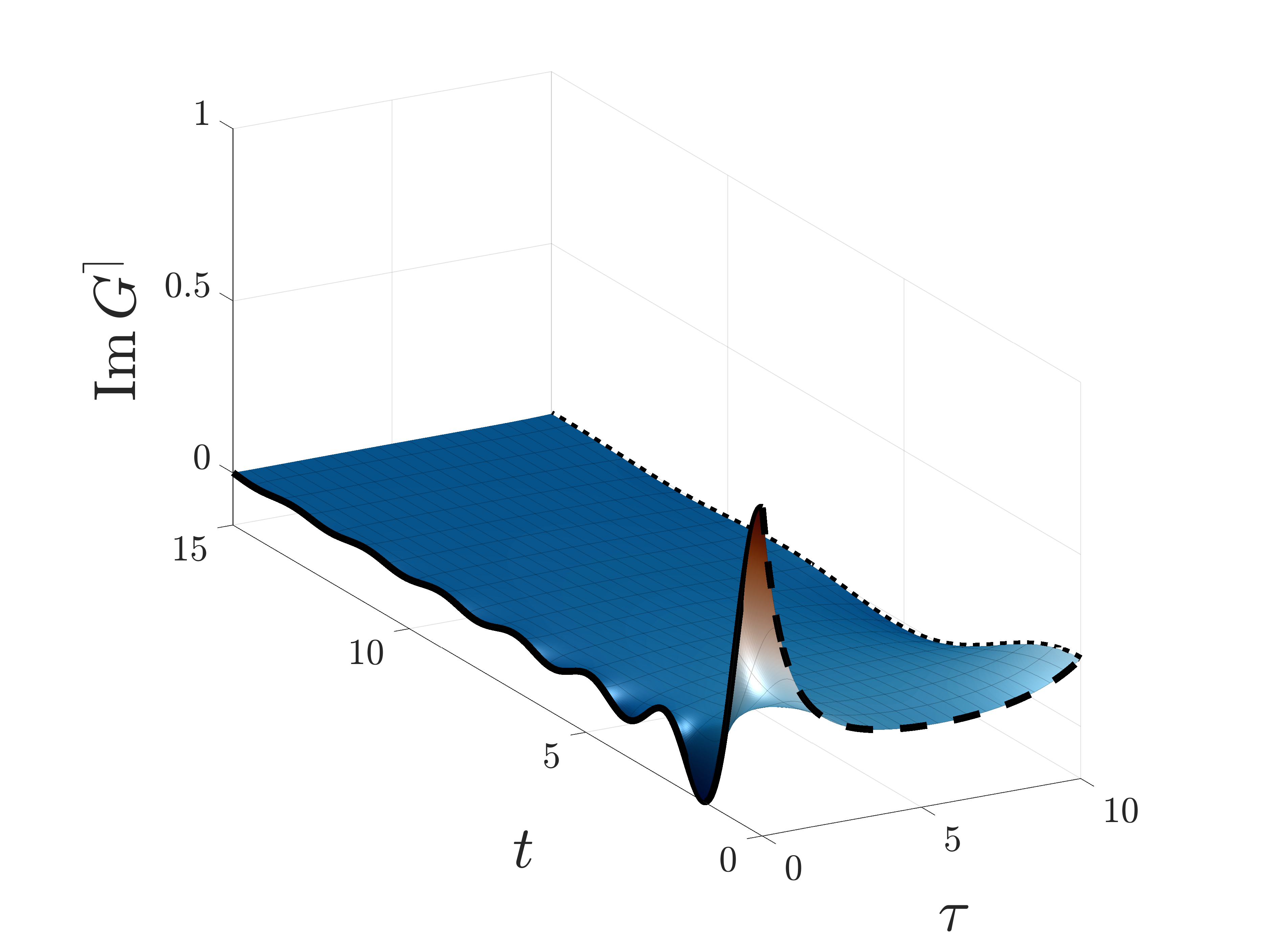
Figure 5: $\operatorname{Im}G^{\rceil}(t,\tau)$ for the Bethe lattice self-consistency. $G^{M}(-\tau)=\operatorname{Im}G^{\rceil}(0,\tau)$ is indicated by the dashed line, $\operatorname{Im}G^{<}(t)=\operatorname{Im}G^{\rceil}(t,0)$ by the solid line, and $-\operatorname{Im}G^{>}(t)=\operatorname{Im}G^{\rceil}(t,\beta)$ by the dotted line.

For the numerical calculations, we fix $c=1$, $h=-1$ and $\beta=10$, and consider the fermionic case $\xi=-1$. Since the initial condition for the real time propagation of $G^{\rceil}(t,\tau)$ in (8) is determined by $G^{M}(\tau)$, we first solve the imaginary time equation of motion (7). The imaginary time axis $\tau\in[0,\beta]$ is discretized using the DLR tolerance $\epsilon=10^{-15}$, and a high energy cutoff $\Lambda=40$, which we have verified is sufficient to eliminate the discretization error in $\tau$ to high accuracy. The resulting DLR contains $r=31$ basis functions and DLR grid points $\tau_{j}$. We obtain $G^{M}(\tau)$ on the DLR grid using the method described in [16] for the equivalent integral form of (7), treating the nonlinearity by a weighted fixed point iteration with pointwise tolerance $10^{-15}$.

We then solve the real time equation of motion (8) for $G^{\rceil}(t,\tau)$ using the high-order Adams-Moulton method described in Appendix A, and compute $G^{R}(t)$ from (10) by evaluating the DLR expansion (15) of $G^{\rceil}$. We use fixed point iteration with a pointwise tolerance $10^{-15}$ for the nonlinear solve. Figure 5 shows a plot of $G^{\rceil}(t,\tau)$ for $t\in[0,15]$. In Figure 6a, we show convergence of the fourth and eighth-order Adams-Moulton methods with respect to $\Delta t$ by comparing the computed value of $G^{R}(t)$ with the exact solution (18) for $t\in[0,1000]$. We then fix $\Delta t=1/64$, sufficient to achieve near machine precision accuracy for all calculations using the eighth-order method, and vary the final propagation time from $t=1$ to $t=131072$ by increasing the number $N$ of time steps. Figure 6b shows wall clock timings using direct history summation (for some choices of $N$) and our fast history summation algorithm. We observe the expected $\mathcal{O}\left(N\log^{2}N\right)$ scaling for the fast method, and note that it is superior for $N\geq 256$, indicating a very small pre-factor in the scaling. For the longest propagation carried out here, with $N=8388608$ and $T=131072$, only $N\approx 110000$ time steps to $T\approx 1700$ would be possible by the direct method with the same cost. We also note that only one fixed point iteration is required to reach self-consistency for all time steps after the first $500$, and before that at most two, indicating that the equations are non-stiff and an Adams predictor-corrector-type method is sufficient in this case [55, Sec 5.4.2.].

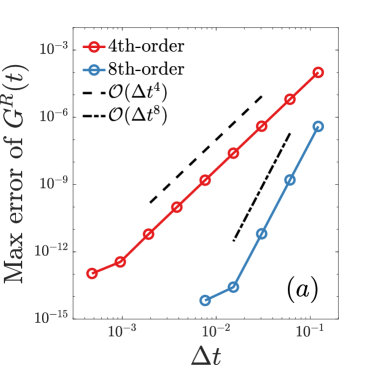
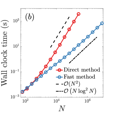
Figure 6: Numerical experiments with the Bethe lattice self-consistency $\Sigma=G$. (a) Convergence of the Adams-Moulton method as $\Delta t\to 0$. (b) Wall clock timings using direct and fast history summation with fixed $\Delta t$ and increasing propagation time.

4.2 The Sachdev-Yitaev-Ke model

The fermionic Sachdev-Yitaev-Ke (SYK) model demonstrates the challenge of resolving emergent low energy features in quantum many-body systems. It is used to model certain features of strange metals, a poorly understood phase of matter with properties distinct from simple metals, and is connected to a variety of other phenomena of physical interest [47, 48, 49, 56, 57]. The SYK equations of motion in real time are given by (7) and (8) with $\xi=-1$, and a self-energy consisting of a single second-order diagram in the interaction $J$, containing a product of three Green’s functions:

$$\Sigma^{M}(\tau) =J^{2}\left(G^{M}(\tau)\right)^{2}G^{M}(\beta-\tau)$$ (19)

$$\Sigma^{\rceil}(t,\tau) =J^{2}\left(G^{\rceil}(t,\tau)\right)^{2}\left(G^{\rceil}(t,\beta-\tau)\right)^{*}.$$

In the limit of zero temperature $T=1/\beta\to 0$, the SYK model displays an emergent low energy feature in the spectral function $A(\omega)=-\frac{1}{\pi}\operatorname{Im}G^{R}(\omega)$: a square root divergence $A(\omega)\sim|\omega|^{-1/2}$ [47]. At finite temperature $T$, the divergence is regularized by thermal fluctuations at frequencies $|\omega|\lesssim T$.

In order to resolve this feature, the Green’s function must be propagated to a large time at low temperature. Our fast history summation algorithm makes this practical. We demonstrate this by solving the SYK equations and computing the spectral density at temperatures up to four orders of magnitude smaller than the coupling strength $J$, and establish the scaling of the cost required to reach even lower temperatures.

We solve the SYK equations and compute $G^{R}(t)$ and $A(\omega)$ for $J=1$, $h=0$ and $\beta=100,1000,10000$ using the eighth-order Adams-Moulton method described in Appendix A. We tune all discretization parameters, and the propagation time, so that the spectral function $A(\omega)$ is resolved.

For $\beta=10000$, we use the DLR parameters $\Lambda=10^{5}$ and $\epsilon=10^{-10}$, which yields $r=92$ degrees of freedom in $\tau$. We use a fixed point tolerance of $10^{-14}$ for the nonlinear iteration. We propagate to a final time $t=50000$ with $N=1048576$ time steps. The computation takes less than five minutes to complete using our fast method. It would take approximately two days by the direct method.

We note that for all three choices of $\beta$, only one fixed point iteration is required to reach self-consistency for all time steps after the first $100$, and before that at most three.

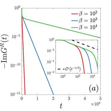
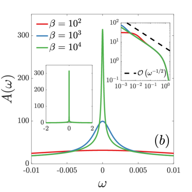
Figure 7: Numerical experiments for the SYK model. (a) Asymptotic behavior of the retarded Green’s function $G^{R}(t)$ at different temperatures. The inital $t^{-1/2}$ decay (inset) transitions into exponential decay at a rate proportional to the temperature, requiring large propagation times for low temperature. (b) Structure of the spectral density $A(\omega)$ at different temperatures. The spectral function becomes highly localized at low temperatures (left inset). In the $\beta\to\infty$ limit, it approaches an $|\omega|^{-1/2}$ singularity at the origin (right inset).

Plots of $G^{R}$ and $A$ are shown in Figure 7. $G^{R}(t)$ decays exponentially as $t\to\infty$ at a rate proportional to the temperature (Figure 7a). As a result, for large $\beta$, the spectral density is highly localized (Figure 7b). In the zero-temperature limit, the spectral density has an $|\omega|^{-1/2}$ singularity at the origin. Although for finite temperature $A(\omega)$ is smooth, we observe it approaching this singularity as $\beta\to\infty$, with a corresponding $t^{-1/2}$ decay regime in $G^{R}(t)$ at intermediate times.

5 Conclusion

We have presented an efficient solver for a class of nonlinear convolutional Volterra integro-differential equations for which the integral kernel depends causally on the solution. As is typical for Volterra-type equations, the computational bottleneck is the evaluation of history integrals at each time step. However, in the present setting, limited knowledge of the kernel at a given time step precludes the use of the various Volterra history summation techniques which have been introduced in the literature. We present an $\mathcal{O}\left(N\log^{2}N\right)$ algorithm which properly handles the structure of the integral operator.

We are motivated to study equations of the form (1) by their appearance in quantum many-body Green’s function methods. In particular, the equilibrium real time Dyson equation of motion (8) for the single particle Green’s function can be reduced to a system of equations of this form. By using the imaginary time Green’s function, which is relatively easy to compute, to initialize real time propagation, our approach requires only local nonlinear iteration. By contrast, the standard method requires global nonlinear iteration in real time and frequency, which can lead to slow convergence in regimes of physical interest.

As proofs of concept, we present numerical experiments for the Bethe graph [45, 46] and the Sachdev-Ye-Kitaev model [47, 49], demonstrating propagation to extremely large times. In particular, we are able to resolve the square root divergence in the SYK model at a temperature $1/\beta$ four orders of magnitude lower than the coupling $J$, $\beta^{-1}/J=10^{-4}$, while resolving energy scales $\omega$ three orders of magnitude smaller than $J$, $\omega/J\approx 10^{-3}$, in a calculation taking less than five minutes on a single CPU core of a laptop. More generally, our approach is applicable to many-body Green’s function methods with low order self-energy expressions, as in low order pertubation theory [1, 2, 3, 4], as well as bubble and ladder resummations like Hedin’s GW approximation and beyond [58, 59, 60, 61].

Appendix A Adams-Moulton time stepping with Gregory integration

We consider a general coupled system of equations of the form (1), in order to directly treat the case of the equilibrium Dyson equation described in Section 3.2:

$$iy_{j}^{\prime}(t)+\int_{0}^{t}k_{j}\left(y_{1}(t-t^{\prime}),\ldots,y_{d}(t-t^{\prime}),t-t^{\prime}\right)y_{j}(t^{\prime})\,dt^{\prime}=f_{j}(y_{1}(t),\ldots,y_{d}(t),t)$$ (20)

for $j=1,\ldots,d$.

We discretize (20) by the Adams-Moulton method. For notational simplicity, we suppress the dependence of $k$ and $f$ on $y_{1},\ldots,y_{d}$, and write

$$\widetilde{f}_{j}(t)\equiv f_{j}(t)-\int_{0}^{t}k_{j}(t-t^{\prime})y_{j}(t^{\prime})\,dt^{\prime}$$

so that

$$iy_{j}^{\prime}(t)=\widetilde{f}_{j}(t).$$

Integrating both sides from $t_{n}$ to $t_{n+1}$ gives

$$y_{j}^{n+1}=y_{j}^{n}-i\int_{t_{n}}^{t_{n+1}}\widetilde{f}_{j}(t)\,dt.$$

The Adams-Moulton method of order $p$ is obtained by replacing the integrand with its polynomial interpolant at the points $\{t_{n+1-j}\}_{j=0}^{p-1}$, and computing the resulting integrals analytically. This yields the discretization

$$y_{j}^{n+1}=y_{j}^{n}-i\Delta t\sum_{l=0}^{p-1}\mu^{\text{AM}}_{l}\widetilde{f}_{j}^{n+1-l}=y_{j}^{n}-i\Delta t\sum_{l=0}^{p-1}\mu^{\text{AM}}_{l}\left(f_{j}^{n+1-l}-\int_{0}^{t_{n+1-l}}k_{j}(t_{n+1-l}-t^{\prime})y_{j}(t^{\prime})\,dt^{\prime}\right).$$ (21)

Here, $\mu^{\text{AM}}_{j}$ are the Adams-Moulton weights. For a procedure to obtain the weights, along with tabulated weights for methods of up to eighth-order, we refer the reader to [62, Chap. 24].

It remains to discretize the history integrals to high-order accuracy. Since $y_{j}(t)$ is known only at the grid points $t=t_{n}$, a standard high-order rule, such as a composite Gauss-Legendre rule, would require interpolation, and is inconsistent with our fast algorithm without significant modification. Instead we require a high-order rule of the form

$$\int_{0}^{t_{n}}k_{j}(t_{n}-t^{\prime})y_{j}(t^{\prime})\,dt^{\prime}\approx\Delta t\sum_{m=0}^{n}k_{j}^{n-m}y_{j}^{m}+\Delta t\sum_{m=0}^{q-1}\mu^{\text{G}}_{m}\left(k_{j}^{n-m}y_{j}^{m}+k_{j}^{m}y_{j}^{n-m}\right)\equiv S_{j}^{n}$$ (22)

for some weights $\mu^{\text{G}}_{m}$; that is, a standard equispaced rule with endpoint corrections. A simple method is the Gregory integration rule. The Gregory rule with $q$ weights is correct to order $q+1$. Although this approach becomes unstable for very high orders, we have found it to be effective at least up to order $8$. More stable endpoint-corrected rules have been introduced, including modifications of Gregory rules [63, 64], and stable rules of very high order which require modifying endpoint node locations [65, 66], but we have found the standard Gregory rules to be sufficient for our purposes. For a procedure to obtain the weights, we refer the reader to [64]; the weights are obtained from the Gregory coefficients, which are tabulated to high order in [67, 68].

Inserting (22) into (21) and rearranging to place all unknown quantities on the left hand side, we obtain

$$\begin{multlined}\left(1-i\Delta t^{2}\mu^{\text{AM}}_{0}\left(1+\mu^{\text{G}}_{0}\right)\right)y_{j}^{n+1}-i\mu^{\text{AM}}_{0}\Delta t^{2}\left(1+\mu^{\text{G}}_{0}\right)k_{j}^{n+1}y_{j}^{0}+i\mu^{\text{AM}}_{0}\Delta tf_{j}^{n+1}\\ =y_{j}^{n}+i\mu^{\text{AM}}_{0}\Delta t\overline{S}_{j}^{n+1}-i\Delta t\sum_{l=1}^{p-1}\mu^{\text{AM}}_{l}\left(f_{j}^{n+1-l}-S_{j}^{n+1-l}\right)\end{multlined}\left(1-i\Delta t^{2}\mu^{\text{AM}}_{0}\left(1+\mu^{\text{G}}_{0}\right)\right)y_{j}^{n+1}-i\mu^{\text{AM}}_{0}\Delta t^{2}\left(1+\mu^{\text{G}}_{0}\right)k_{j}^{n+1}y_{j}^{0}+i\mu^{\text{AM}}_{0}\Delta tf_{j}^{n+1}\\ =y_{j}^{n}+i\mu^{\text{AM}}_{0}\Delta t\overline{S}_{j}^{n+1}-i\Delta t\sum_{l=1}^{p-1}\mu^{\text{AM}}_{l}\left(f_{j}^{n+1-l}-S_{j}^{n+1-l}\right)$$ (23)

where we have defined the truncated endpoint-corrected history sum

$$\overline{S}_{j}^{n}\equiv S_{j}^{n}-\Delta t\left(k_{j}^{n}y_{j}^{0}+k_{j}^{0}y_{j}^{n}+\mu^{\text{G}}_{0}\left(k_{j}^{n}y_{j}^{0}+k_{j}^{0}y_{j}^{n}\right)\right).$$ (24)

This is a collection of $d$ coupled nonlinear equations, which are closed by prescribing the functional dependence of $k_{j}^{n}$ and $f_{j}^{n}$ on $y_{1}^{n},\ldots,y_{d}^{n}$. Once these are solved, $S_{j}^{n+1}$ must be computed by updating the value $\overline{S}_{j}^{n+1}$ using (24). In any given time step, the previous $p-1$ computed values of $f_{j}^{n}$ and $S_{j}^{n}$ must be stored, along with the full history of $y_{j}$, for $j=1,\ldots,d$.

We can split the endpoint corrected history sums $S_{j}^{n}$ into two terms, $S_{j}^{n}=\Delta t\left(s_{j}^{n}+c_{j}^{n}\right)$, with

$$s_{j}^{n}\equiv\sum_{m=0}^{n}k_{j}^{n-m}y_{j}^{m},$$

a standard equispaced history sum, and

$$c_{j}^{n}\equiv\sum_{m=0}^{q-1}\mu^{\text{G}}_{m}\left(k_{j}^{n-m}y_{j}^{m}+k_{j}^{m}y_{j}^{n-m}\right),$$

a local correction. Thus, as for the simple discretization given in Section 2, we recognize the computation of the sums $s_{j}^{n}$ as the quadratic scaling bottleneck of the time stepping procedure, and we can apply the same fast algorithm.

We do not suggest a specific nonlinear iteration procedure to solve (23) – in our numerical examples, we use a simple fixed point iteration – but propose using an Adams-Bashforth method to obtain an initial guess. The Adams-Bashforth method is derived in a similar manner to the Adams-Moulton method, but it is explicit. The $p$th order Adams-Bashforth discretization is given by

$$\begin{multlined}y_{j}^{n+1}=y_{j}^{n}-i\Delta t\sum_{l=1}^{p}\mu^{\text{AB}}_{l}\left(f_{j}^{n+1-l}-S_{j}^{n+1-l}\right).\end{multlined}y_{j}^{n+1}=y_{j}^{n}-i\Delta t\sum_{l=1}^{p}\mu^{\text{AB}}_{l}\left(f_{j}^{n+1-l}-S_{j}^{n+1-l}\right).$$ (25)

We again refer the reader to [62, Chap. 24] for a method to compute the Adams-Bashforth weights $\mu^{\text{AB}}$, along with tabulated weights for the methods up to eighth-order. In practice, using this guess can significantly reduce the number of nonlinear iterations required at each time step.

To obtain a method of order $p$, it suffices to set $q=p-1$. Then (23) is only applicable when $n\geq p-2$, and (25) when $n\geq p-1$. An alternative method is then required to obtain $y_{j}^{n}$, $f_{j}^{n}$, and $S_{j}^{n}$ for $n=0,\ldots,p-1$. A convenient approach is to use Richardson extrapolation on the second-order version of the method – the implicit trapezoidal rule – which does not require any initialization. The method, which requires $p$ to be even, proceeds as follows:

1. Use the second-order method, (23), with $p=2$, until a final time $t=(p-1)\Delta t$, taking time steps of size $\Delta t$, $\Delta t/2$, $\Delta t/4$, …, $\Delta t/2^{p/2-1}$. Record the computed values of $y_{j}^{n}$, $f_{j}^{n}$, and $S_{j}^{n}$ for each time step choice.

2. Apply Richardson extrapolation to these values to obtain approximations of $y_{j}(t)$, $f_{j}(t)$, and $S_{j}(t)$ at $t=\Delta t,2\Delta t,\ldots,(p-1)\Delta t$ which are accurate to order $p$.

Here, we have used that the truncation error of the implicit trapezoidal rule contains only even-order terms. For further details of the Richardson extrapolation procedure, we refer the reader to [69, Sec. 3.4.6].

Appendix B Fast application of square, triangular, and parallelogram-shaped Toeplitz blocks

We first review the standard fast algorithm to apply an $n\times n$ Toeplitz matrix $A$ in $\mathcal{O}\left(n\log n\right)$ operations [70, Sec. 4.7.7]. Let $D$ be the $n\times n$ discrete Fourier transform matrix, $D_{jk}=\omega_{n}^{jk}$ with $\omega_{n}=e^{-2\pi i/n}$, and let $C$ be an $n\times n$ circulant matrix with first column $c$. Then $D$ diagonalizes $C$:

$$C=D^{-1}\Phi D.$$

Here $\Phi$ is the diagonal matrix with entries $Dc$. Since $D$ and $D^{-1}$ can be applied to a vector in $\mathcal{O}\left(n\log n\right)$ operations using the FFT, this gives an $\mathcal{O}\left(n\log n\right)$ algorithm to compute a matrix-vector product $b=Cx$:

1:Compute $Dc$ by FFT

2:Compute $Dx$ by FFT

3:Compute the entrywise product $Dc\odot Dx$

4:Compute $b=D^{-1}\left(Dc\odot Dx\right)$ by inverse FFT

Algorithm 3 Fast matrix-vector product $b=Cx$ for a circulant matrix $C$ with first column $c$

To obtain an $\mathcal{O}\left(n\log n\right)$ algorithm to compute the product $b=Ax$ with an $n\times n$ Toeplitz matrix $A$, we simply embed $A$ in a $2n\times 2n$ circulant matrix $C$, apply $C$ to a zero-padded vector $x$ using Algorithm 3, and truncate the result. An example for $n=4$ illustrates the method:

$$\left(\begin{array}[]{cccc|cccc}\bf{d}&\bf{c}&\bf{b}&\bf{a}&0&g&f&e\\ \bf{e}&\bf{d}&\bf{c}&\bf{b}&a&0&g&f\\ \bf{f}&\bf{e}&\bf{d}&\bf{c}&b&a&0&g\\ \bf{g}&\bf{f}&\bf{e}&\bf{d}&c&b&a&0\\ \hline\cr 0&g&f&e&d&c&b&a\\ a&0&g&f&e&d&c&b\\ b&a&0&g&f&e&d&c\\ c&b&a&0&g&f&e&d\\ \end{array}\right)\left(\begin{array}[]{c}\bf{x_{1}}\\ \bf{x_{2}}\\ \bf{x_{3}}\\ \bf{x_{4}}\\ \hline\cr 0\\ 0\\ 0\\ 0\\ \end{array}\right)=\left(\begin{array}[]{c}\bf{b_{1}}\\ \bf{b_{2}}\\ \bf{b_{3}}\\ \bf{b_{4}}\\ \hline\cr-\\ -\\ -\\ -\\ \end{array}\right).$$

Here, the top-left block, with bolded entries, is the original Toeplitz matrix $A$, which has been extended to a circulant matrix. The vector $x$ is zero-padded as shown. Then, the result is truncated; here, the desired result is the vector $b=(b_{1}\,\,b_{2}\,\,b_{3}\,\,b_{4})^{T}$, and the dashes indicate entries that are ignored.

A triangular Toeplitz matrix is simply a special case of a square Toeplitz matrix; in the above example, we would take $e=f=g=0$. Therefore the algorithm for this case is the same.

We could also treat the case of a Toeplitz matrix whose non-zero entries form a parallelogram as simply another special case. However, this requires forming a circulant matrix of approximately twice the size necessary. We illustrate a more efficient method using the example of a $4\times 7$ parallelogram:

$$\left(\begin{array}[]{cccccccc}\bf{d}&\bf{c}&\bf{b}&\bf{a}&0&0&0\\ 0&\bf{d}&\bf{c}&\bf{b}&\bf{a}&0&0\\ 0&0&\bf{d}&\bf{c}&\bf{b}&\bf{a}&0\\ 0&0&0&\bf{d}&\bf{c}&\bf{b}&\bf{a}\\ \hline\cr a&0&0&0&d&c&b\\ b&a&0&0&0&d&c\\ c&b&a&0&0&0&d\\ \end{array}\right)\left(\begin{array}[]{c}\bf{x_{1}}\\ \bf{x_{2}}\\ \bf{x_{3}}\\ \bf{x_{4}}\\ \bf{x_{5}}\\ \bf{x_{6}}\\ \bf{x_{7}}\\ \end{array}\right)=\left(\begin{array}[]{c}\bf{b_{1}}\\ \bf{b_{2}}\\ \bf{b_{3}}\\ \bf{b_{4}}\\ \hline\cr-\\ -\\ -\\ \end{array}\right).$$

Here, the parallelogram has been embedded in the top half of a circulant matrix. No zero-padding of the input vector is necessary, but the result is still truncated to obtain $b$.

References

- [1] A. A. Abrikosov, L. P. Gorkov, and I. E. Dzyaloshinski, Methods of Quantum Field Theory in Statistical Physics. Dover Publications, 1965.
- [2] A. L. Fetter and J. D. Walecka, Quantum Theory of Many-Particle Systems. Dover Publications, 2003.
- [3] J. W. Negele and H. Orland, Quantum Many-Particle Systems. Westview Press, 1998.
- [4] G. Stefanucci and R. van Leeuwen, Nonequilibrium Many-Body Theory of Quantum Systems: A Modern Introduction. Cambridge University Press, 2013.
- [5] N.-E. Dahlen and R. van Leeuwen, “Self-consistent solution of the Dyson equation for atoms and molecules within a conserving approximation,” J. Chem. Phys., vol. 122, no. 16, p. 164102, 2005.
- [6] L. Boehnke, H. Hafermann, M. Ferrero, F. Lechermann, and O. Parcollet, “Orthogonal polynomial representation of imaginary-time Green’s functions,” Phys. Rev. B, vol. 84, p. 075145, 2011.
- [7] E. Gull, S. Iskakov, I. Krivenko, A. A. Rusakov, and D. Zgid, “Chebyshev polynomial representation of imaginary-time response functions,” Phys. Rev. B, vol. 98, p. 075127, 2018.
- [8] X. Dong, D. Zgid, E. Gull, and H. U. R. Strand, “Legendre-spectral Dyson equation solver with super-exponential convergence,” J. Chem. Phys., vol. 152, no. 13, p. 134107, 2020.
- [9] W. Ku, Electronic excitations in metals and semiconductors: Ab initio studies of realistic many-particle systems. PhD thesis, University of Tennessee, 2000.
- [10] W. Ku and A. G. Eguiluz, “Band-gap problem in semiconductors revisited: Effects of core states and many-body self-consistency,” Phys. Rev. Lett., vol. 89, p. 126401, 2002.
- [11] A. A. Kananenka, J. J. Phillips, and D. Zgid, “Efficient temperature-dependent Green’s functions methods for realistic systems: Compact grids for orthogonal polynomial transforms,” J. Chem. Theory Comput., vol. 12, no. 2, pp. 564–571, 2016.
- [12] H. Shinaoka, J. Otsuki, M. Ohzeki, and K. Yoshimi, “Compressing Green’s function using intermediate representation between imaginary-time and real-frequency domains,” Phys. Rev. B, vol. 96, no. 3, p. 035147, 2017.
- [13] N. Chikano, J. Otsuki, and H. Shinaoka, “Performance analysis of a physically constructed orthogonal representation of imaginary-time Green’s function,” Phys. Rev. B, vol. 98, no. 3, p. 035104, 2018.
- [14] J. Li, M. Wallerberger, N. Chikano, C.-N. Yeh, E. Gull, and H. Shinaoka, “Sparse sampling approach to efficient ab initio calculations at finite temperature,” Phys. Rev. B, vol. 101, no. 3, p. 035144, 2020.
- [15] H. Shinaoka, N. Chikano, E. Gull, J. Li, T. Nomoto, J. Otsuki, M. Wallerberger, T. Wang, and K. Yoshimi, “Efficient ab initio many-body calculations based on sparse modeling of Matsubara Green’s function,” SciPost Phys. Lect. Notes, p. 63, 2022.
- [16] J. Kaye, K. Chen, and O. Parcollet, “Discrete Lehmann representation of imaginary time Green’s functions,” Phys. Rev. B, vol. 105, p. 235115, 2022.
- [17] N.-E. Dahlen, R. van Leeuwen, and A. Stan, “Propagating the Kadanoff-Baym equations for atoms and molecules,” J. Phys. Conf. Ser., vol. 35, pp. 340–348, 2006.
- [18] A. Stan, N.-E. Dahlen, and R. van Leeuwen, “Time propagation of the Kadanoff-Baym equations for inhomogeneous systems,” J. Chem. Phys., vol. 130, no. 22, p. 224101, 2009.
- [19] H. Aoki, N. Tsuji, M. Eckstein, M. Kollar, T. Oka, and P. Werner, “Nonequilibrium dynamical mean-field theory and its applications,” Rev. Mod. Phys., vol. 86, pp. 779–837, 2014.
- [20] N. W. Talarico, S. Maniscalco, and N. Lo Gullo, “A scalable numerical approach to the solution of the Dyson equation for the non-equilibrium single-particle Green’s function,” Phys. Status Solidi B, vol. 256, no. 7, p. 1800501, 2019.
- [21] M. Schüler, D. Golež, Y. Murakami, N. Bittner, A. Herrmann, H. U. R. Strand, P. Werner, and M. Eckstein, “NESSi: The Non-Equilibrium Systems Simulation package,” Comput. Phys. Commun., vol. 257, p. 107484, 2020.
- [22] J. Kaye and D. Golež, “Low rank compression in the numerical solution of the nonequilibrium Dyson equation,” SciPost Phys., vol. 10, p. 91, 2021.
- [23] H. U. R. Strand, M. Eckstein, and P. Werner, “Beyond the Hubbard bands in strongly correlated lattice bosons,” Phys. Rev. A, vol. 92, p. 063602, Dec 2015.
- [24] D. Foerster, P. Koval, and D. Sánchez-Portal, “An implementation of Hedin’s GW approximation for molecules,” J. Chem. Phys., vol. 135, no. 7, p. 074105, 2011.
- [25] U. von Barth and B. Holm, “Self-consistent results for the electron gas: Fixed screened potential within the random-phase approximation,” Phys. Rev. B, vol. 54, pp. 8411–8419, 1996.
- [26] B. Holm and U. von Barth, “Fully self-consistent self-energy of the electron gas,” Phys. Rev. B, vol. 57, pp. 2108–2117, 1998.
- [27] M. Jarrell and J. E. Gubernatis, “Bayesian inference and the analytic continuation of imaginary-time quantum Monte Carlo data,” Physics Reports, vol. 269, pp. 133–195, 5 1996.
- [28] J. Fei, C.-N. Yeh, and E. Gull, “Nevanlinna analytical continuation,” Phys. Rev. Lett., vol. 126, p. 056402, 2021.
- [29] J. Fei, C.-N. Yeh, D. Zgid, and E. Gull, “Analytical continuation of matrix-valued functions: Carathéodory formalism,” Phys. Rev. B, vol. 104, p. 165111, 2021.
- [30] Z. Huang, E. Gull, and L. Lin, “Robust analytic continuation of Green’s functions via projection, pole estimation, and semidefinite relaxation,” Phys. Rev. B, vol. 107, p. 075151, 2023.
- [31] E. Hairer, C. Lubich, and M. Schlichte, “Fast numerical solution of nonlinear Volterra convolution equations,” SIAM J. Sci. Comput., vol. 6, no. 3, pp. 532–541, 1985.
- [32] B. Alpert, L. Greengard, and T. Hagstrom, “Rapid evaluation of nonreflecting boundary kernels for time-domain wave propagation,” SIAM J. Numer. Anal., vol. 37, no. 4, pp. 1138–1164, 2000.
- [33] S. Jiang and L. Greengard, “Fast evaluation of nonreflecting boundary conditions for the Schrödinger equation in one dimension,” Comput. Math. Appl., vol. 47, no. 6, pp. 955–966, 2004.
- [34] S. Jiang and L. Greengard, “Efficient representation of nonreflecting boundary conditions for the time-dependent Schrödinger equation in two dimensions,” Commun. Pure Appl. Math., vol. 61, no. 2, pp. 261–288, 2008.
- [35] S. Jiang, L. Greengard, and S. Wang, “Efficient sum-of-exponentials approximations for the heat kernel and their applications,” Adv. Comput. Math., vol. 41, pp. 529–551, 2015.
- [36] S. Veerapaneni and G. Biros, “A high-order solver for the heat equation in 1d domains with moving boundaries,” SIAM J. Sci. Comput., vol. 29, no. 6, pp. 2581–2606, 2007.
- [37] J.-R. Li, “A fast time stepping method for evaluating fractional integrals,” SIAM J. Sci. Comput., vol. 31, no. 6, pp. 4696–4714, 2010.
- [38] J. Wang, L. Greengard, S. Jiang, and S. Veerapaneni, “Fast integral equation methods for linear and semilinear heat equations in moving domains,” 2019. arXiv:1910.00755.
- [39] J. Kaye, A. Barnett, and L. Greengard, “A high-order integral equation-based solver for the time-dependent Schrödinger equation,” Commun. Pure Appl. Math., vol. 75, no. 8, pp. 1657–1712, 2022.
- [40] J. G. Hoskins, J. Kaye, M. Rachh, and J. C. Schotland, “A fast, high-order numerical method for the simulation of single-excitation states in quantum optics,” J. Comput. Phys., vol. 473, p. 111723, 2023.
- [41] C. Lubich and A. Schädle, “Fast convolution for non–reflecting boundary conditions,” SIAM J. Sci. Comput., vol. 24, pp. 161–182, 2002.
- [42] A. Schädle, M. López-Fernández, and C. Lubich, “Fast and oblivious convolution quadrature,” SIAM J. Sci. Comput., vol. 28, no. 2, pp. 421–438, 2006.
- [43] J. Dölz, H. Egger, and V. Shashkov, “A fast and oblivious matrix compression algorithm for Volterra integral operators,” Adv. Comput. Math., vol. 47, no. 6, pp. 1–24, 2021.
- [44] J. Kaye and L. Greengard, “Transparent boundary conditions for the time-dependent Schrödinger equation with a vector potential,” 2018. arXiv:1812.04200.
- [45] E. N. Economou, Green’s Functions in Quantum Physics. Springer-Verlag, 1983.
- [46] A. Georges, G. Kotliar, W. Krauth, and M. J. Rozenberg, “Dynamical mean-field theory of strongly correlated fermion systems and the limit of infinite dimensions,” Rev. Mod. Phys., vol. 68, no. 1, pp. 13–125, 1996.
- [47] S. Sachdev and J. Ye, “Gapless spin-fluid ground state in a random quantum Heisenberg magnet,” Phys. Rev. Lett., vol. 70, pp. 3339–3342, May 1993.
- [48] D. Chowdhury, A. Georges, O. Parcollet, and S. Sachdev, “Sachdev-Ye-Kitaev models and beyond: Window into non-Fermi liquids,” Rev. Mod. Phys., vol. 94, p. 035004, 2022.
- [49] Y. Gu, A. Kitaev, S. Sachdev, and G. Tarnopolsky, “Notes on the complex Sachdev-Ye-Kitaev model,” J. High Energy Phys., vol. 2020, no. 2, p. 157, 2020.
- [50] H. Cheng, Z. Gimbutas, P.-G. Martinsson, and V. Rokhlin, “On the compression of low rank matrices,” SIAM J. Sci. Comput., vol. 26, no. 4, pp. 1389–1404, 2005.
- [51] E. Liberty, F. Woolfe, P.-G. Martinsson, V. Rokhlin, and M. Tygert, “Randomized algorithms for the low-rank approximation of matrices,” Proc. Natl. Acad. Sci. U.S.A., vol. 104, no. 51, pp. 20167–20172, 2007.
- [52] J. Kaye, K. Chen, and H. U. R. Strand, “libdlr: Efficient imaginary time calculations using the discrete Lehmann representation,” Comput. Phys. Commun., vol. 280, p. 108458, 2022.
- [53] https://github.com/jasonkaye/libdlr.
- [54] M. Frigo and S. G. Johnson, “The design and implementation of FFTW3,” Proc. IEEE, vol. 93, no. 2, pp. 216–231, 2005.
- [55] U. Ascher and L. Petzold, Computer Methods for Ordinary Differential Equations and Differential-Algebraic Equations. Society for Industrial and Applied Mathematics, 1998.
- [56] L. García-Álvarez, I. L. Egusquiza, L. Lamata, A. del Campo, J. Sonner, and E. Solano, “Digital quantum simulation of minimal ,” Phys. Rev. Lett., vol. 119, p. 040501, 2017.
- [57] C. Wei and T. A. Sedrakyan, “Optical lattice platform for the Sachdev-Ye-Kitaev model,” Phys. Rev. A, vol. 103, p. 013323, 2021.
- [58] L. Hedin, “New method for calculating the one-particle Green’s function with application to the electron-gas problem,” Phys. Rev., vol. 139, no. 3A, 1965.
- [59] D. Golze, M. Dvorak, and P. Rinke, “The compendium: A practical guide to theoretical photoemission spectroscopy,” Front. Chem., vol. 7, p. 377, 2019.
- [60] G. Stefanucci, Y. Pavlyukh, A.-M. Uimonen, and R. van Leeuwen, “Diagrammatic expansion for positive spectral functions beyond : Application to vertex corrections in the electron gas,” Phys. Rev. B, vol. 90, p. 115134, 2014.
- [61] A. L. Kutepov, “Electronic structure of and from a self-consistent vertex-corrected approach,” Phys. Rev. B, vol. 104, p. 085109, 2021.
- [62] J. Butcher, Numerical Methods for Ordinary Differential Equations. Wiley, 2016.
- [63] B. Fornberg and J. A. Reeger, “An improved Gregory-like method for 1-d quadrature,” Numer. Math., vol. 141, no. 1, pp. 1–19, 2019.
- [64] B. Fornberg, “Improving the accuracy of the trapezoidal rule,” SIAM Rev., vol. 63, pp. 167–180, 2021.
- [65] S. Kapur and V. Rokhlin, “High-order corrected trapezoidal quadrature rules for singular functions,” SIAM J. Numer. Anal., vol. 34, no. 4, pp. 1331–1356, 1997.
- [66] B. K. Alpert, “Hybrid Gauss-trapezoidal quadrature rules,” SIAM J. Sci. Comput., vol. 20, no. 5, pp. 1551–1584, 1999.
- [67] OEIS Foundation Inc., “The On-Line Encyclopedia of Integer Sequences.” http://oeis.org/A002206, 2021.
- [68] OEIS Foundation Inc., “The On-Line Encyclopedia of Integer Sequences.” http://oeis.org/A002207, 2021.
- [69] G. Dahlquist and A. Björck, Numerical Methods in Scientific Computing: Volume 1. SIAM, 2008.
- [70] G. Golub and C. Van Loan, Matrix Computations. Johns Hopkins University Press, 3 ed., 1996.